From Prediction to Decision: Leakage-Controlled Machine Learning with Uncertainty-Calibrated Black-Litterman Allocation

Abstract

Machine-learning (ML) portfolio studies often emphasize forecast accuracy, although economic value depends on how forecasts propagate through uncertainty, constraints, turnover, and transaction costs. We evaluate a leakage-controlled decision-support pipeline combining weekly Elastic Net and Random Forest excess-return forecasts with uncertainty-calibrated Black–Litterman (BL) allocation across five ETFs. Data from 2021–2023 form the training sample, 2024 is used for walk-forward selection and confidence calibration, and 2025 is a final 53-week holdout; model coefficients may update with newly observed data, but the configuration is frozen before the holdout. Neither pooled ML model beats the zero or historical-mean forecasts on the pre-specified Mean NRMSE. BL–Elastic Net obtains a net Sharpe ratio of 2.762 with 0.86% average weekly turnover and a −3.11% maximum drawdown; descriptively, its Sharpe exceeds 1/N (2.425) and mean–variance (2.324) but not GMV (3.069). However, circular block-bootstrap 95% confidence intervals for all BL–Elastic Net and BL–Random Forest Sharpe differences versus 1/N, GMV, and mean–variance include zero. Sensitivity, regime, and implementation analyses therefore support a bounded conclusion: forecast ranking and portfolio ranking can diverge, but the available holdout does not establish statistically significant risk-adjusted dominance.

1. Introduction

Portfolio allocation is an intelligent decision problem under uncertainty: expected returns are latent, volatility and dependence structures change over time, and any forecast must ultimately be converted into constrained actions that incur implementation costs. Classical mean–variance theory formalized the diversification problem [1], but practical optimization is highly sensitive to estimated expected returns and covariance inputs [2,3]. The Black–Litterman (BL) framework mitigates part of this instability by combining a structured prior with uncertain views [4], while the empirical resilience of simple allocation rules such as 1/N remains a demanding benchmark for more sophisticated methods [5].

Machine learning (ML) can enlarge the information-processing capacity of the allocation system and represent interactions that are difficult to capture with low-dimensional linear models. Yet prediction and decision are not equivalent objectives. A small reduction in forecasting error may be economically irrelevant if it causes concentrated allocations, high turnover, unstable exposures, or gains that disappear after costs. Conversely, a weak but stable signal may become useful when it is filtered through a prior, scaled by estimated uncertainty, and translated into weights under explicit constraints. This distinction is especially important in financial markets, where public information is rapidly incorporated into prices [6,7] and predictive relations may evolve across regimes [8].

The general ML-finance literature has documented nonlinear predictability in asset-pricing data [9], the use of AI in asset management [10], and a broad range of intelligent portfolio-management techniques [11]. Decision-oriented studies have also translated machine-learned forecasts into portfolio weights [12,13]. More specifically, the growing literature couples data-driven forecasts with BL views. Barua and Sharma use CNN–BiLSTM predictions as dynamic BL views [14]; Li et al. develop a Random-Forest-based BL formulation [15]; Barua and Sharma combine sentiment-related signals and XGBoost with BL [16]; Hung et al. integrate BERT-derived news sentiment and recurrent neural networks into the BL view distribution [17]; and Su et al. propose a deep-learning hybrid for objective BL views [18]. These studies establish that ML-generated BL views can be useful, but they also mean that simply combining ML and BL is not, by itself, a sufficient novelty claim.

The motivation is decision-system rather than forecasting-centric. A portfolio manager or an intelligent decision-support system does not consume RMSE directly; it consumes allocations that must be stable, auditable, implementable, and robust to uncertainty. The practical question is therefore whether a predictive signal remains useful after it is filtered by a prior, discounted according to its historical reliability, constrained by portfolio rules, and charged for the trading that it induces. This is the gap addressed here.

Accordingly, the study has four explicit objectives. O1 quantifies whether Elastic Net or Random Forest improves one-week-ahead excess-return prediction relative to zero and expanding-historical-mean forecasts under a leakage-controlled holdout. O2 separates forecast value from decision-layer value by passing the same forecasts through an uncertainty-calibrated BL allocation and comparing the resulting portfolios with 1/N, GMV, and traditional mean–variance. O3 measures implementability through turnover, transaction costs, drawdown, concentration, and tail risk. O4 tests whether the qualitative conclusions survive perturbations in pooling, estimation window, covariance estimator, BL parameters, view-confidence calibration, and market regime.

We evaluate this architecture using weekly one-step-ahead excess-return forecasts for five heterogeneous ETFs. Forecasts enter BL as absolute views, confidence is calibrated from prior out-of-sample forecast errors, and posterior expected returns are mapped to long-only, fully invested portfolios with a common 40% asset cap. The empirical design separates 2021–2023 training, 2024 walk-forward validation, and a final 2025 holdout that is never used for ex-post specification selection. The five-ETF universe is intentionally compact but spans U.S. and non-U.S. equities, intermediate Treasuries, gold, and Treasury bills. The 2021–2025 sample contains materially different environments—the 2021 reopening/vaccine phase, the 2022 inflation and Russia–Ukraine shock, the 2022–2023 monetary-tightening cycle, and the subsequent disinflation/rate-normalization phase—but this heterogeneity does not make the sample universally representative; external validity remains limited by the small universe and the one-year final holdout.

The contribution is therefore an evaluation architecture rather than a new forecasting algorithm. First, predictive accuracy and economic decision quality are evaluated separately, allowing the experiment to detect prediction–decision divergence rather than assuming that lower error implies a better portfolio. Second, forecast uncertainty is explicitly propagated into the BL layer and frozen before the final holdout. Third, implementation quality is evaluated through turnover, transaction costs, drawdown, tail loss, and concentration, not only terminal return. Fourth, robustness is examined across pooled and asset-specific models, feature sets, expanding and rolling windows, covariance estimators, BL parameters, view-confidence calibrations, and market regimes. Finally, statistical uncertainty is assessed using a circular block bootstrap that preserves short-range temporal dependence.

This design produces a deliberately cautious empirical result. In the primary 2025 specification, neither pooled ML model beats simple predictive benchmarks on the pre-specified Mean NRMSE criterion, and global minimum variance remains the strongest portfolio on net Sharpe ratio. Nevertheless, BL–Elastic Net improves on 1/N and traditional mean–variance in risk-adjusted performance while maintaining low turnover. The result is informative precisely because it does not rely on universal ML dominance: it identifies a boundary condition under which decision-layer filtering can add value even when raw predictive superiority is weak.

The remainder of the paper is organized as follows. Section 2 positions the study relative to ML-driven BL allocation and decision-support research. Section 3 describes the data, leakage-controlled validation protocol, predictive models, uncertainty-calibrated BL layer, benchmarks, and statistical evaluation. Section 4 reports predictive, economic, and robustness results. Section 5 interprets the findings and discusses engineering implications and limitations. Section 6 concludes.

2. Related Work and Research Contribution

Three studies intersect in this study. The first concerns predictive learning in noisy financial time series. Random Forests are flexible ensemble learners for nonlinear interactions [19], whereas Elastic Net combines L1 and L2 regularization and is useful when predictors are correlated and the sample is limited [20]. In time-series applications, however, model evaluation must respect temporal ordering: random cross-validation and repeated specification search can create leakage or backtest overfitting [21,22]. The relevant question is therefore not how well a model fits historical data, but how a pre-specified learning protocol generalizes to information that was genuinely unavailable during model selection.

The second study addresses input uncertainty in portfolio optimization. Mean–variance weights can respond aggressively to small perturbations of expected returns [2,3]. BL provides a natural information-fusion layer because it does not require a forecast to become a portfolio weight directly: a forecast enters as a view whose influence depends on its uncertainty [4,23]. This separation is central to the present design. It allows the same predictive signal to be attenuated when prior out-of-sample error is large, thereby making forecast reliability an explicit engineering variable in the decision system.

The third study directly combines ML or deep learning with BL. Existing studies have generated absolute or relative BL views using deep neural networks, Random Forests, XGBoost, sentiment analysis, and hybrid forecasting architectures [14,15,16,17,18]. Several report substantial portfolio outperformance. The present study is complementary rather than duplicative: it intentionally uses two standard models of different complexity, a small multi-asset universe, and simple benchmarks to test whether apparent predictive sophistication survives a frozen holdout, transaction costs, uncertainty calibration, robustness perturbations, and statistical uncertainty. In particular—refer to Table 1—the paper does not claim novelty for Random-Forest-generated BL views; its contribution lies in the leakage-controlled and decision-oriented evaluation of the whole pipeline.

Table 1. Positioning relative to closely related ML–Black–Litterman studies.

Study	Signal/View Construction	Portfolio Layer	Relevance to the Present Study
Barua and Sharma [14]	CNN–BiLSTM price predictions and technical indicators	Dynamic BL	Shows the potential of deep forecasts as BL views; the present study instead stresses frozen-holdout evaluation and prediction–decision divergence.
Li et al. [15]	Random-Forest-generated views	RF-based BL with multi-objective optimization	Establishes prior art for RF–BL integration; the present contribution is therefore not the RF–BL pairing itself.
Barua and Sharma [16]	XGBoost return forecasts plus fear/greed signal	BL with relative views	Demonstrates richer sentiment-informed views; the present study deliberately uses a compact information set to emphasize validation and implementability.
Hung et al. [17]	BERT news sentiment with RNN/LSTM/GRU forecasts	BL view distribution	Shows value from unstructured information; the present study focuses on uncertainty calibration and leakage control with structured data.
Su et al. [18]	CEEMDAN, GA-optimized LSTM, and LSTM aggregation	Hybrid CGL–BL	Represents a high-complexity predictive architecture; the present experiment tests whether simpler regularized signals can remain competitive after decision-layer filtering.
This study	Elastic Net and Random Forest weekly excess-return forecasts	Error-calibrated BL; common constraints and costs	Separates predictive from decision quality; freezes the holdout design; tests turnover, costs, regimes, sensitivity, and block-bootstrap uncertainty.

3. Materials and Methods

3.1. Investment Universe, Data Sources, and Temporal Design

The investable universe contains five exchange-traded funds chosen to represent distinct components of a simple multi-asset portfolio: SPY (U.S. equities), EFA (developed equities outside the United States), IEF (intermediate U.S. Treasury bonds), GLD (gold), and BIL (short-duration U.S. Treasury bills). Daily market data are obtained from Yahoo Finance [24], using adjusted closing prices for return calculations and retaining trading volume. Macroeconomic and market-risk variables are obtained from the Federal Reserve Bank of St. Louis FRED database [25], including VIXCLS, DGS2, DGS10, and DTB3. When a macroeconomic series is subject to publication delay or revision, the design principle is to use only information actually available at the decision date.

Daily observations cover 4 January 2021 through 31 December 2025. Weekly observations are formed using the adjusted closing price from the last available trading session of each week rather than an average of daily prices. The final aligned dataset contains 261 common weekly observations for each ETF: 156 weeks in 2021–2023, 52 weeks in 2024, and 53 weeks in 2025. After maturation of the longest 12-week features and alignment of the one-week-ahead target, the initial 2021–2023 training panel contains 143 target weeks per ETF, or 715 pooled supervised rows; across the full study horizon there are 1240 complete asset-week rows. No price interpolation or automatic winsorization is applied. Extreme returns are retained because they are economically relevant to downside and tail-risk measures.

The sample is divided chronologically into three non-interchangeable blocks. The 2021–2023 training sample is used for initial fitting and feature construction. The 2024 validation sample is used for walk-forward hyperparameter selection, comparison of model specifications, and calibration of BL view uncertainty. The 2025 final holdout is reserved for the concluding out-of-sample evaluation. Model configurations and BL calibration rules are frozen at the end of 2024; during 2025, models may be re-estimated only with observations that have become available up to each forecast date.

The weekly decision clock is explicit. At the last available trading session of week t, all market variables and FRED series are cut off at observations dated no later than that session; if a series has no observation on that day, the latest earlier observation is carried forward. The final predictor set uses daily market or market-rate series (VIXCLS, DGS2, DGS10, and DTB3), so no later monthly or quarterly vintage is backfilled into an earlier decision. Features are computed from information through the close of week t, the forecast targets the close-to-close interval from week t to week $t+1$, target weights are computed after the forecast, and those weights are evaluated only on the subsequent realized week.

DTB3 is quoted on a 360-day bank-discount basis. The weekly risk-free proxy used throughout the experiment is

$$r_t^f=\left({\displaystyle \frac{\mathrm{DTB}{3}_t}{100}}\right){\displaystyle \frac{7}{360}}.$$

(1)

The dependent variable is the one-week-ahead simple ETF return minus this decision-date weekly proxy. The same $r_t^f$ enters the weekly excess-return series used for Sharpe and Sortino calculations. This convention is intentionally simple and internally consistent; it is not presented as a full bond-equivalent-yield conversion. The empirical design and temporal separation is summed up in Table 2.

Table 2. Empirical design and temporal separation.

Period	Role	Main Operations	Leakage Control
2021–2023	Training	Initial model estimation, feature construction, internal walk-forward errors	Only contemporaneously available information
2024	Validation	Hyperparameter selection, model comparison, calibration of view uncertainty Ω	Sequential walk-forward; no 2025 information
2025	Final holdout	Final predictive and portfolio evaluation	Configuration frozen before holdout; no ex-post retuning

Prediction Target and Predictor Set

For each ETF i, the prediction target is the one-week-ahead excess return. The risk-free proxy is the three-month U.S. Treasury bill rate (DTB3), converted from its annualized discount-basis quotation to a weekly equivalent. BIL remains an investable asset, whereas DTB3 is used as the risk-free reference for the target and risk-adjusted performance metrics.

Here and below, “one-week-ahead” always means the next observed weekly close-to-close interval, and the 360-day convention and $7/360$ conversion above are used consistently for the target and risk-adjusted metrics.

$$y_{i,t+1}=r_{i,t+1}-r_t^f.$$

(2)

The information set is deliberately compact to match the limited sample size. Asset-specific variables include the lagged weekly return, four- and twelve-week momentum, realized volatility over four and twelve weeks, twelve-week drawdown, and a volume-change indicator. Market and macrofinancial variables include the VIX level and its four-week change, the ten-year Treasury yield and its four-week change, the ten-minus-two-year yield spread, and the three-month Treasury bill rate. ETF identity dummies allow the pooled model to distinguish asset classes. All features observed at week t are used to predict week t + 1; continuous variables used by Elastic Net are standardized using parameters estimated only from data available at that time. The predictive variables used are summed up in Table 3.

Table 3. Predictive variables used in the full specification.

Group	Variables	Purpose
Return dynamics	Return ($t-1$), momentum 4 weeks, momentum 12 weeks	Short- and medium-horizon persistence/reversal
Risk	Realized volatility 4 and 12 weeks; drawdown 12 weeks	Recent and persistent risk conditions
Liquidity/attention	Volume change relative to moving average	Trading intensity
Market risk	VIX level; VIX four-week change	Risk aversion and changes in expected volatility
Rates/curve	DGS10; four-week DGS10 change; DGS10-DGS2; DTB3	Long rate, rate shock, curve slope, monetary conditions
Asset identity	ETF binary indicators	Heterogeneity across asset classes

3.2. Predictive Models, Software Implementation, and Validation

Two supervised regressors are compared. Elastic Net provides a linear, strongly regularized and interpretable baseline [20]. Its penalty intensity $\lambda$ is selected from {${10}^{-4}$, ${10}^{-3}$, ${10}^{-2}$, ${10}^{-1}$, 1}, and the L1/L2 mixing parameter is selected from {0.1, 0.5, 0.9}. Random Forest provides the nonlinear alternative [19]. Its parsimonious grid contains 200 or 500 trees, maximum depth {3, 5, 8}, minimum leaf size {5, 10, 20}, and candidate-feature fractions equal to the square root of the feature count, 50%, or 100%; squared error is used as the split loss.

All predictive models were implemented in Python using scikit-learn version 1.8.0 [26], specifically the ElasticNet and RandomForestRegressor estimators. The same temporally aligned dataset and the same decision calendar are used for both models. The Random Forest does not require feature standardization, whereas Elastic Net is standardized at each decision date using moments estimated only from the data then available. Model coefficients and tree-based feature importances are used for interpretation only and are not treated as causal evidence.

The main specification pools the five ETFs in one panel so that the models share information across assets while retaining ETF indicators. This increases the number of supervised rows relative to fitting five completely separate models. Separate per-ETF models are nevertheless evaluated as a robustness check. Hyperparameters are selected by walk-forward validation on 2024. Because the ETFs have materially different volatilities, the primary selection criterion is the unweighted average across assets of RMSE normalized by the training-sample standard deviation of each target (Mean NRMSE). Pooled RMSE, pooled MAE, directional accuracy, and out-of-sample $R^2$ against simple benchmarks are reported as complementary measures. When performance is essentially tied, the less complex configuration is preferred.

The 2024 validation selects a Random Forest with 500 trees, maximum depth 3, and at least 20 observations per leaf. For Elastic Net, the strongly regularized solution contracts the pooled coefficients to zero in the selected configuration, making it effectively conservative. This outcome is not overridden by inspecting 2025: the frozen model-selection rule is part of the experimental design.

This point changes the interpretation of the result. In the selected pooled Elastic Net, all penalized slope coefficients—including the ETF-indicator coefficients—are zero, while the standard unpenalized intercept remains. Consequently, at any decision date the five Elastic Net forecasts reduce to the same pooled intercept; that intercept is not fixed for the year because it is re-estimated as the expanding sample grows. BL–Elastic Net is therefore a time-updated common-view strategy, not an asset-ranking Elastic Net strategy. Its 53.96% directional accuracy may partly reflect the unconditional frequency of positive excess-return weeks rather than cross-sectional forecasting skill. We retain the specification because it was selected by the pre-specified 2024 validation rule; replacing it after observing 2025 would violate the holdout design.

Leakage-Controlled Walk-Forward Protocol

The empirical pipeline follows expanding-window walk-forward estimation. At each weekly decision date, the system (1) forms predictors using information available through that date; (2) standardizes variables from the current estimation sample; (3) estimates or updates the predictive model; (4) generates one-week-ahead excess-return forecasts; (5) converts them into BL views; (6) computes target portfolio weights; (7) applies those weights to the subsequent realized weekly returns; and (8) adds the newly realized observation to the estimation set. A 104-week rolling window is used only as a pre-specified robustness test.

This design separates adaptive learning from retrospective respecification. Updating a model with newly observed 2025 data is permitted because those data were available at the next decision date; changing hyperparameters, feature definitions, BL confidence rules, or benchmark selection because of the observed 2025 performance is not.

In short, the configuration is frozen, not the fitted coefficients: each 2025 weekly fit may incorporate only observations already realized by that date, while hyperparameters, feature definitions, confidence rules, constraints, and the identity of the reported primary specification remain fixed at their end-2024 values.

This distinction is essential in low signal-to-noise financial applications, where repeated specification search can produce backtest overfitting [21,22].

3.3. Uncertainty-Calibrated Black–Litterman Decision Layer

The ML forecasts do not become portfolio weights directly. Instead, they enter BL as absolute views. The reference portfolio is a neutral equal-weight strategic prior because assets represent heterogeneous market segments and ETF assets-under-management would not be a meaningful proxy for the global economic weight of the underlying asset classes. Let ${\mathbf{\Sigma }}_t$ denote the weekly covariance matrix estimated with the expanding window and let ${\mathbf{w}}^0$ denote the equal-weight prior. The implied excess-return vector is

$${\mathit{\pi }}_t=\delta {\mathbf{\Sigma }}_t{\mathbf{w}}^0,\delta =3.$$

(3)

The five ML predictions form ${\mathbf{q}}_t$ and $\mathbf{P}=\mathbf{I}$. View uncertainty Ω is diagonal and is calibrated from out-of-sample forecasting errors:

$$\mathbf{\Omega }=\mathrm{diag}\left({\widehat{\sigma }}_{e,1}^2,\dots ,{\widehat{\sigma }}_{e,5}^2\right),$$

(4)

where ${\widehat{\sigma }}_{e,i}^2$ is the out-of-sample forecast-error variance for asset i. For 2024, these variances are estimated using internal walk-forward predictions from the earlier sample; at the end of 2024, Ω is recalibrated using validation errors and then frozen for 2025. Thus, a less accurate forecast receives a larger uncertainty variance and exerts less influence on the posterior [23]. The BL posterior mean is

$${\mathit{\mu }}_t^{\mathrm{BL}}={\left[{\left(\tau {\mathbf{\Sigma }}_t\right)}^{-1}+{\mathbf{P}}^{\top }{\mathbf{\Omega }}^{-1}\mathbf{P}\right]}^{-1}\left[{\left(\tau {\mathbf{\Sigma }}_t\right)}^{-1}{\mathit{\pi }}_t+{\mathbf{P}}^{\top }{\mathbf{\Omega }}^{-1}{\mathbf{q}}_t\right],\tau =0.05.$$

(5)

The baseline portfolio is obtained by maximizing the mean–variance objective using the BL posterior while imposing long-only, fully invested, no-leverage weights and a 40% upper bound per asset:

$$\begin{array}{cc}\hfill \underset{\mathbf{w}}{\max }& {\mathbf{w}}^{\top }{\mathit{\mu }}_t^{\mathrm{BL}}-{\displaystyle \frac{\delta }{2}}{\mathbf{w}}^{\top }{\mathbf{\Sigma }}_t\mathbf{w}\hfill \\ \hfill \mathrm{s}.\mathrm{t}.& {\mathbf{1}}^{\top }\mathbf{w}=1,0\le w_i\le 0.40.\hfill \end{array}$$

(6)

The risk matrix in Equation (6) is the same expanding-window sample covariance ${\mathbf{\Sigma }}_t$ used by GMV and traditional mean–variance. We deliberately do not substitute the BL posterior covariance in the objective: holding the risk estimator common across optimized strategies isolates the effect of changing expected-return information and view confidence. A posterior-covariance allocation would answer a different question and is left as an extension.

Two diagnostic controls clarify the BL contribution. With no views, the posterior mean collapses to ${\mathit{\pi }}_t=\delta {\mathbf{\Sigma }}_t{\mathbf{w}}^0$; because ${\mathbf{w}}^0={(0.2,\dots ,0.2)}^{\top }$ satisfies the 40% cap, Equation (6) returns ${\mathbf{w}}^0$, so the no-view BL control is exactly 1/N. In the selected Elastic Net specification, the zero slopes imply the time-updated common-view signal described above; hence BL–Elastic Net is already the common-view diagnostic. We do not add a newly tuned historical-mean-as-BL-view strategy after observing 2025 because it was not part of the pre-specified holdout comparison; the expanding historical mean remains the predictive benchmark, while traditional mean–variance already uses expanding historical means as expected-return inputs.

Sensitivity tests vary maximum asset weight $w_{\max }\in \{0.30,0.40,0.50\}$, risk-aversion coefficient $\delta \in \{2,3,5\}$, prior-uncertainty scale $\tau \in \{0.025,0.05,0.10\}$, covariance estimator (sample or Ledoit–Wolf shrinkage [27]), and view-confidence calibration (forecast-error MSE or view variance). These are one-at-a-time perturbations of the pre-specified baseline, not an ex-post search for the most favorable 2025 configuration. Figure 1 reports end-to-end machine-learning and the Black–Litterman decision-support pipeline (Algorithm 1).

Algorithm 1: Leakage-controlled weekly forecast-to-allocation loop

At the end of week t, assemble only predictors whose values are observable by that decision time. Fit or update the selected predictive model using the expanding historical sample; standardize Elastic Net inputs using training-window moments only. Generate one-week-ahead excess-return forecasts ${\mathbf{q}}_t$ for the five ETFs. Combine the forecasts with the strategic prior ${\mathit{\pi }}_t$ through the BL posterior, using the pre-calibrated view-error matrix Ω. Solve the constrained allocation problem with long-only, fully invested weights and the common asset cap. Apply transaction costs to the one-way turnover required to move from drifted pre-rebalancing weights to the new target weights. Observe week $t+1$ returns, record predictive and portfolio metrics, and only then append the new observation to the estimation sample.

Figure 1. End-to-end machine-learning and Black–Litterman decision-support pipeline.

3.4. Evaluation, Robustness, and Statistical Uncertainty

Forecasting benchmarks are (i) a zero expected excess-return forecast and (ii) the expanding historical mean. Portfolio benchmarks use the same long-only, fully invested, 40% cap whenever optimization is required. GMV solves

$$\underset{\mathbf{w}}{\min }{\mathbf{w}}^{\top }{\mathbf{\Sigma }}_t\mathbf{w},{\mathbf{1}}^{\top }\mathbf{w}=1,0\le w_i\le 0.40,$$

(7)

with the same expanding-window sample covariance used by BL. Traditional mean–variance uses the expanding historical mean vector ${\overline{\mathbf{r}}}_t$ as expected returns and maximizes ${\mathbf{w}}^{\top }{\overline{\mathbf{r}}}_t-(\delta /2){\mathbf{w}}^{\top }{\mathbf{\Sigma }}_t\mathbf{w}$ under the same constraints. Equal weight (1/N) is the non-optimized benchmark.

For forecasting,

$${\mathrm{NRMSE}}_i={\displaystyle \frac{\sqrt{T^{-1}{\sum }_t{(y_{i,t}-{\widehat{y}}_{i,t})}^2}}{s_i^{\mathrm{train}}}},\mathrm{Mean}\mathrm{NRMSE}={\displaystyle \frac{1}{5}}{\displaystyle \sum _{i=1}^5}{\mathrm{NRMSE}}_i,$$

(8)

where $s_i^{\mathrm{train}}$ is the standard deviation of the aligned 2021–2023 one-week-ahead target for ETF i (143 target weeks per ETF). This denominator is fixed before validation and holdout evaluation.

Let $R_{p,t}^{\mathrm{net}}$ be weekly portfolio return after costs and $x_t=R_{p,t}^{\mathrm{net}}-r_t^f$. With T weeks,

$$R_{\mathrm{ann}}={\left[{\displaystyle \prod _{t=1}^T}(1+R_{p,t}^{\mathrm{net}})\right]}^{52/T}-1,{\sigma }_{\mathrm{ann}}=\sqrt{52}\mathrm{sd}\left(R_{p,t}^{\mathrm{net}}\right),$$

(9)

$$\mathrm{Sharpe}=\sqrt{52}{\displaystyle \frac{\overline{x}}{\mathrm{sd}\left(x_t\right)}},\mathrm{Sortino}=\sqrt{52}{\displaystyle \frac{\overline{x}}{\sqrt{T^{-1}{\sum }_t\min {(x_t,0)}^2}}}.$$

(10)

The annual return is geometric, whereas Sharpe ([28,29]) uses the arithmetic mean and standard deviation of weekly excess returns with the time-varying DTB3 proxy. Consequently, the reported Sharpe cannot be reproduced by simply dividing annualized return by annualized volatility.

Transaction costs are charged per unit of one-way turnover measured relative to the pre-rebalancing portfolio weights after market drift. The baseline is 10 basis points, with 5 and 20 basis points used for sensitivity analysis. This makes turnover an economic variable rather than a descriptive afterthought, consistent with evidence that implementability can materially alter conclusions from characteristic- or signal-based strategies [30].

Pooled RMSE, pooled MAE, directional accuracy, and out-of-sample $R^2$ are complementary forecast measures. Risk and implementation metrics include Maximum Drawdown, weekly Expected Shortfall at 95% [31,32], worst weekly return, positive-week frequency, average turnover, maximum asset weight, and the Herfindahl concentration index. Statistical uncertainty in strategy comparisons is assessed with a circular block bootstrap using 5000 replications and four-week blocks [33]. This is the primary dependence-robust inference for portfolio differences. Given only 53 holdout weeks, we do not add a second post hoc asymptotic Sharpe-difference test whose small-sample approximation would be fragile. Likewise, H1 is interpreted from the pre-specified loss metrics rather than from a newly introduced post hoc Diebold–Mariano/Clark–West testing layer; no claim of statistically significant predictive dominance is made.

3.4.1. Pre-Specified Hypotheses

The empirical design is organized around four hypotheses.

Hypothesis 1. 

Tests whether at least one ML model improves the pre-specified Mean NRMSE relative to the zero and expanding-historical-mean forecasting benchmarks in the final holdout.

Hypothesis 2. 

Tests whether integrating ML views into BL improves net risk-adjusted portfolio performance relative to traditional portfolio benchmarks.

Hypothesis 3. 

Tests whether any economic advantage persists when transaction costs vary from 5 to 20 basis points per unit of one-way turnover.

Hypothesis 4. 

Tests whether the qualitative conclusions remain stable across pre-specified variations in pooling, feature sets, estimation windows, covariance estimation, BL parameters, view confidence, and market regimes.

3.4.2. Market-Regime Analysis

Three one-dimensional regime classifications are defined using rules fixed from the training sample. Volatility is classified as low or high according to whether the VIX is below or above the training-sample median. The equity regime uses the sign of 13-week SPY momentum. The rates regime uses the 13-week change in the ten-year Treasury yield, with the ten-minus-two-year spread as complementary context. Regimes are not crossed with one another because the one-year final holdout would then generate samples too small for meaningful interpretation. The regime analysis is therefore descriptive and robustness-oriented rather than a separate model-selection exercise.

4. Results

4.1. Data Integrity and Predictive Evidence

All five ETFs have 1255 valid daily observations and 261 aligned weekly observations over the study horizon. After lag construction and the one-step-ahead target, the pooled supervised panel contains 1240 complete rows across the full period. Quality checks cover date consistency, duplicates, price fields, the FRED macrofinancial series, and the temporal availability of predictors.

The 2024 validation results show that simple forecasting benchmarks are difficult to beat. The selected Random Forest improves on Elastic Net but does not outperform the benchmarks under the pre-defined Mean NRMSE criterion. Its feature-importance profile is dominated by momentum and realized-volatility variables, which jointly account for roughly three quarters of the model’s importance; macrofinancial inputs play a secondary role and ETF dummies are marginal. These importances are descriptive rather than causal.

Final-Holdout Predictive Performance

The final 2025 holdout contains 53 weekly decisions and 265 asset-level forecasts. Table 4 reports the frozen-model results. The expanding historical mean obtains the lowest Mean NRMSE (0.9471), followed by the zero benchmark (0.9508). Random Forest reaches 1.1417 and Elastic Net 1.7674. On the primary criterion, neither pooled ML model therefore dominates the simple benchmarks. Directional accuracy is also not improved: the historical mean reaches 57.74%, versus 53.96% for Elastic Net and 52.45% for Random Forest.

Table 4. Predictive performance in the final holdout (2025).

Model	Mean NRMSE	Pooled RMSE	Pooled MAE	Directional Accuracy	OOS ${\mathit{R}}^2$ vs. Zero	OOS ${\mathit{R}}^2$ vs. Hist. Mean
Zero	0.9508	0.01902	0.01214	—	—	−0.0213
Historical mean	0.9471	0.01882	0.01201	57.74%	0.0208	—
Elastic Net	1.7674	0.01891	0.01218	53.96%	0.0118	−0.0093
Random Forest	1.1417	0.01889	0.01212	52.45%	0.0137	−0.0073

Mean NRMSE and pooled RMSE answer different questions. Mean NRMSE first scales each ETF’s error by its fixed training-target standard deviation and then gives the five assets equal weight; pooled RMSE aggregates errors in return units and therefore gives more influence to high-volatility assets. This explains why Elastic Net is much worse than the zero forecast on Mean NRMSE (1.7674 versus 0.9508) while being slightly better on pooled RMSE (0.01891 versus 0.01902). BIL is especially influential after normalization because its excess-return target has a very small training standard deviation: small absolute errors can therefore generate a large NRMSE. The same scale issue affects Ω differently because confidence is calibrated in absolute squared-return units. Mean NRMSE remains the pre-specified cross-asset criterion; pooled metrics are complementary, not interchangeable.

This result is important for the interpretation of the portfolio experiment. Any economic improvement from the ML-assisted strategies cannot be attributed to a general forecasting victory by the frozen pooled models. It must instead arise from how weak or noisy signals interact with the prior, forecast-error confidence, covariance structure, and portfolio constraints.

4.2. Economic Performance and Implementability

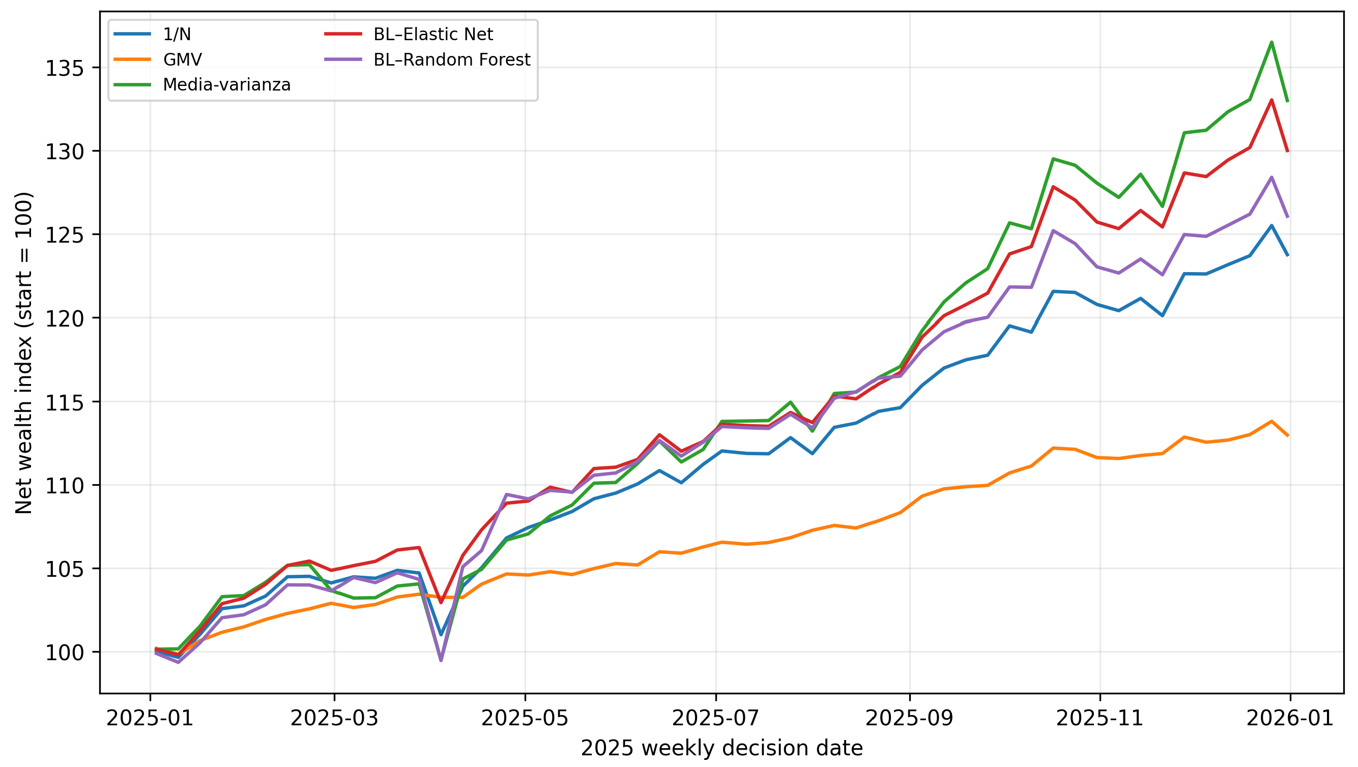
Table 5 summarizes net portfolio performance in the 2025 holdout under the 10 bps baseline cost. No strategy dominates every dimension. Mean–variance produces the highest annualized net return (32.29%) but also substantially higher volatility (10.54%). GMV produces the strongest risk-adjusted performance, with a Sharpe ratio of 3.069 and volatility of only 2.58%. Among the ML-assisted strategies, BL–Elastic Net achieves a 29.36% annualized net return, 7.97% volatility, and a Sharpe ratio of 2.762. Descriptively, this Sharpe is above 1/N (2.425) and mean–variance (2.324) and below GMV (3.069); however, all circular block-bootstrap 95% confidence intervals for the corresponding Sharpe differences include zero, so this ordering is not statistically established. BL–Random Forest reaches a 25.51% annualized net return and a Sharpe ratio of 1.950.

Table 5. Net economic performance in the final holdout (2025; 10 bps cost).

Strategy	Cumulative Net Return	Annualized Net Return	Annualized Volatility	Net Sharpe	Net Sortino
1/N	23.76%	23.27%	7.05%	2.425	3.979
GMV	12.98%	12.72%	2.58%	3.069	6.231
Mean–variance	33.00%	32.29%	10.54%	2.324	4.027
BL–Elastic Net	30.00%	29.36%	7.97%	2.762	4.918
BL–Random Forest	26.06%	25.51%	9.82%	1.950	3.447

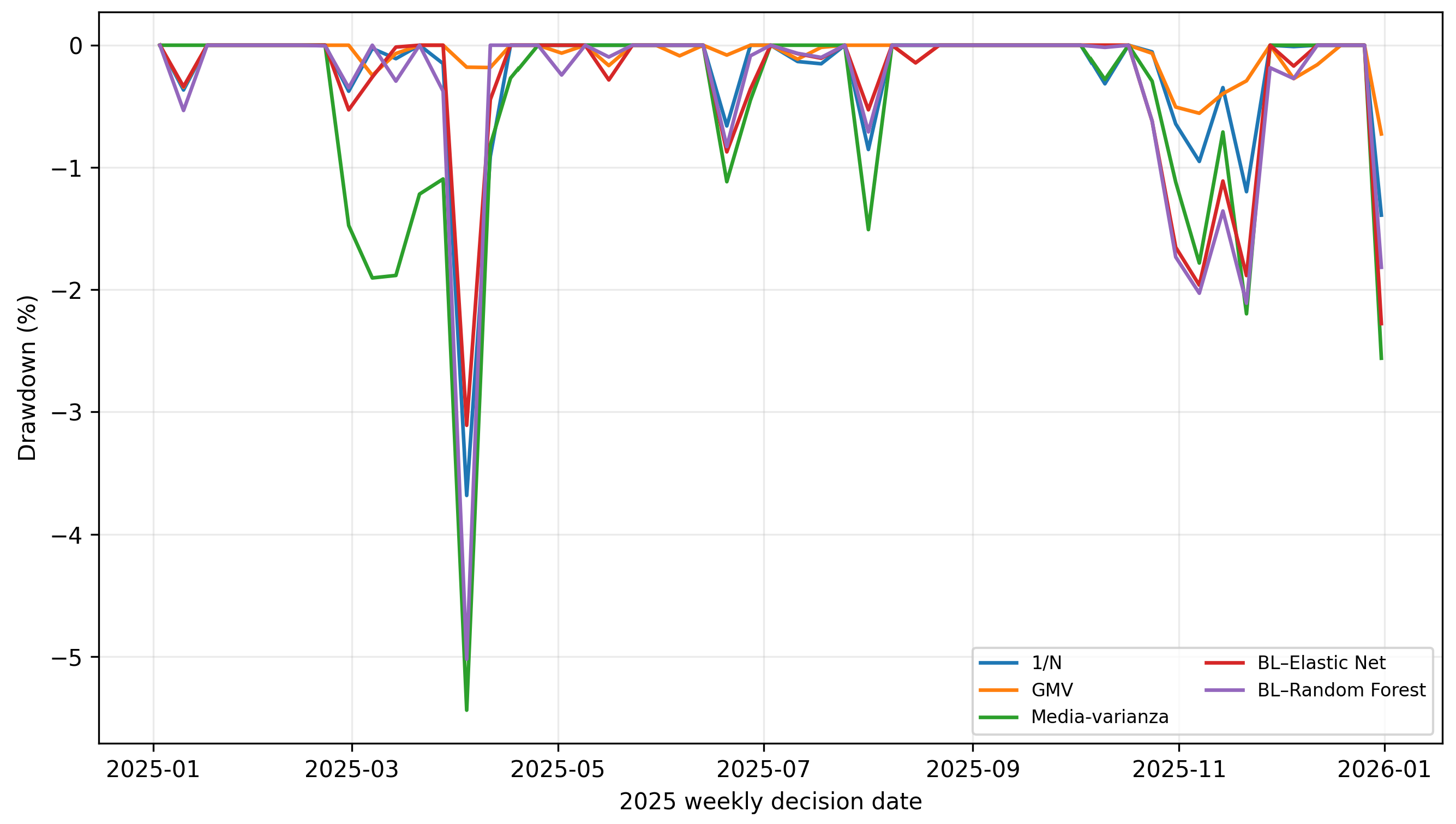
Figure 2 reports cumulative net wealth paths in the 2025 final holdout (initial wealth index = 100). Instead, Figure 3 reports the drawdown paths of the five portfolio strategies in the 2025 final holdout.

Figure 2. Cumulative net wealth paths in the 2025 final holdout (initial wealth index = 100).

Figure 3. Drawdown paths of the five portfolio strategies in the 2025 final holdout.

The central empirical finding is thus a prediction–decision divergence. Elastic Net is not the best forecaster in the main specification, yet its forecasts, after being shrunk by the BL prior and error-calibrated Ω, generate a competitive portfolio. By contrast, Random Forest provides a more reactive nonlinear signal but does not obtain a commensurate increase in risk-adjusted portfolio performance.

4.2.1. Risk, Turnover, and Concentration

Implementation metrics explain a substantial part of this divergence. BL–Elastic Net has an average weekly turnover of only 0.86%, compared with 13.87% for BL–Random Forest. Over the 53-week holdout, this corresponds to cumulative turnover of approximately 45.4% versus 734.9%, respectively. The Random Forest strategy therefore trades a notional amount equivalent to about 7.35 times the portfolio capital over the year, exposing it much more heavily to costs and model instability.

BL–Elastic Net also records a Maximum Drawdown of −3.11%, better than 1/N (−3.68%), mean–variance (−5.44%), and BL–Random Forest (−5.02%), although GMV is substantially more defensive at −0.73%. Weekly Expected Shortfall at 95% is −2.14% for BL–Elastic Net and −2.53% for BL–Random Forest. These results reinforce the point that a portfolio model should be judged not only by terminal return or forecasting error but also by the path and cost of implementation.

Table 6 reports the turnover, and concentration in the 2025 final holdout.

Table 6. Risk, turnover, and concentration in the 2025 final holdout.

Strategy	Maximum Drawdown	ES 95% (Weekly)	Worst Week	Positive Weeks	Avg. Weekly Turnover	HHI	Max Weight
1/N	−3.68%	−1.93%	−3.53%	69.81%	0.57%	0.200	20.00%
GMV	−0.73%	−0.50%	−0.73%	71.70%	0.39%	0.339	40.00%
Mean–variance	−5.44%	−2.82%	−4.39%	79.25%	1.94%	0.356	40.00%
BL–Elastic Net	−3.11%	−2.14%	−3.11%	71.70%	0.86%	0.271	38.17%
BL–Random Forest	−5.02%	−2.53%	−4.66%	62.26%	13.87%	0.243	40.00%

4.2.2. Transaction-Cost Sensitivity

The cost sensitivity in Table 7 shows two distinct operating profiles. BL–Elastic Net is nearly invariant as costs increase from 5 to 20 bps because its weights change slowly: the net Sharpe ratio moves only from 2.764 to 2.757. BL–Random Forest declines from 1.985 to 1.879 over the same cost range. GMV remains the best risk-adjusted benchmark throughout the tested cost levels.

Table 7. Net Sharpe ratio under alternative transaction-cost assumptions.

Strategy	5 bps	10 bps	20 bps
1/N	2.4266	2.4247	2.4208
GMV	3.0729	3.0690	3.0612
Mean–variance	2.3287	2.3239	2.3142
BL–Elastic Net	2.7642	2.7619	2.7573
BL–Random Forest	1.9849	1.9497	1.8790

4.3. Robustness, Regimes, and Hypothesis Assessment

Robustness tests qualify, rather than overturn, the main findings. When Random Forests are estimated separately for each ETF, Mean NRMSE improves to 0.9404, marginally better than the historical mean (0.9471) and zero benchmark (0.9508). The corresponding BL–Random Forest portfolio, however, has a net Sharpe ratio of 2.1709 and 21.25% average weekly turnover. For Elastic Net, the 104-week rolling-window portfolio has a Sharpe ratio of 2.4253, versus 2.4247 for 1/N at the same 10 bps cost; the equality at three decimals in the previous manuscript was only a rounding coincidence.

Table 8 reports the BL architecture sensitivity numerically. Replacing the baseline forecast-error-MSE Ω with view variance increases BL–Elastic Net’s Sharpe from 2.7619 to 2.9289 and turnover from 0.86% to 1.81%, but reduces BL–Random Forest’s Sharpe from 1.9497 to 1.1293 while increasing turnover from 13.87% to 28.60%. Ledoit–Wolf covariance shrinkage lowers Sharpe for both ML-assisted portfolios in this sample. These rows are sensitivity diagnostics, not candidates for ex-post replacement of the baseline.

Table 8. Black–Litterman architectural sensitivity in the 2025 holdout.

Test	Value	Strategy	Role	Net Sharpe	Turnover/wk.	MDD
$w_{\max }$	0.30	BL–EN	sensitivity	2.7429	0.83%	n/a †
$w_{\max }$	0.30	BL–RF	sensitivity	2.0144	12.02%	n/a †
$w_{\max }$	0.40	BL–EN	baseline	2.7619	0.86%	−3.11%
$w_{\max }$	0.40	BL–RF	baseline	1.9497	13.87%	−5.02%
$w_{\max }$	0.50	BL–EN	sensitivity	2.7619	0.86%	n/a †
$w_{\max }$	0.50	BL–RF	sensitivity	1.9175	14.47%	n/a †
$\delta$	2	BL–EN	sensitivity	2.7595	0.95%	n/a †
$\delta$	2	BL–RF	sensitivity	1.8035	15.56%	n/a †
$\delta$	3	BL–EN	baseline	2.7619	0.86%	−3.11%
$\delta$	3	BL–RF	baseline	1.9497	13.87%	−5.02%
$\delta$	5	BL–EN	sensitivity	2.7298	1.02%	n/a †
$\delta$	5	BL–RF	sensitivity	2.0961	11.28%	n/a †
$\tau$	0.025	BL–EN	sensitivity	2.6826	0.89%	n/a †
$\tau$	0.025	BL–RF	sensitivity	2.1397	9.90%	n/a †
$\tau$	0.05	BL–EN	baseline	2.7619	0.86%	−3.11%
$\tau$	0.05	BL–RF	baseline	1.9497	13.87%	−5.02%
$\tau$	0.10	BL–EN	sensitivity	2.8387	1.11%	n/a †
$\tau$	0.10	BL–RF	sensitivity	1.7476	17.67%	n/a †
Covariance	sample	BL–EN	baseline	2.7619	0.86%	−3.11%
Covariance	sample	BL–RF	baseline	1.9497	13.87%	−5.02%
Covariance	Ledoit–Wolf	BL–EN	sensitivity	2.2949	0.55%	n/a †
Covariance	Ledoit–Wolf	BL–RF	sensitivity	1.8013	15.92%	n/a †
Ω	error MSE	BL–EN	baseline	2.7619	0.86%	−3.11%
Ω	error MSE	BL–RF	baseline	1.9497	13.87%	−5.02%
Ω	view variance	BL–EN	sensitivity	2.9289	1.81%	n/a †
Ω	view variance	BL–RF	sensitivity	1.1293	28.60%	n/a †

Note: Baseline MDD is shown in the final column. ^† The archived one-at-a-time sensitivity output retains annual return, Sharpe, and turnover but not path-level returns for the non-baseline sensitivity runs; therefore their MDDs cannot be reconstructed without rerunning the original experiment and are not inferred from aggregate statistics. The full retained sensitivity extract is supplied as Supplementary Data S1.

The rates-regime results omitted from the previous manuscript are now reported with the volatility and equity regimes in Table 9. The small regime counts (especially $N=14$ and $N=19$) make these comparisons exploratory only.

Table 9. Net Sharpe ratio by pre-defined 2025 market regime.

Dimension	Regime	N	1/N	GMV	MV	BL–EN	BL–RF
Volatility	Low	34	2.5393	2.7935	2.6888	3.1176	2.3682
Volatility	High	19	2.6009	3.4584	2.1513	2.4805	2.0197
Equity momentum	Positive	39	2.9238	3.4544	2.6739	3.0598	2.5988
Equity momentum	Negative	14	1.7010	1.8036	1.6780	2.0347	1.4966
Rates	Rising	23	3.4946	4.3666	2.5704	4.0407	3.4107
Rates	Falling/stable	30	2.0618	2.3522	2.3077	2.3298	1.6609

Table 10 reports the requested circular block-bootstrap Sharpe differences. Every 95% interval includes zero; hence Table 5’s descriptive ranking is not statistical proof of Sharpe superiority.

Table 10. Circular block-bootstrap differences in net Sharpe (5000 replications; four-week blocks).

ML Strategy	Benchmark	Difference	95% CI Lower	95% CI Upper
BL–EN	1/N	0.3372	−0.5771	0.9853
BL–EN	GMV	−0.3071	−1.5739	0.9265
BL–EN	MV	0.4380	−0.2923	1.1839
BL–RF	1/N	−0.4750	−1.1600	0.0181
BL–RF	GMV	−1.1193	−2.6936	0.3425
BL–RF	MV	−0.3742	−1.1018	0.5832

Table 11 reports the outcomes of the pre-specified hypotheses. The hypothesis assessment therefore supports a bounded conclusion: decision-layer filtering can create economically useful behavior in some configurations, but the evidence does not justify a claim that ML universally improves either prediction or portfolio performance.

Table 11. Outcomes of the pre-specified hypotheses.

Hypothesis	Outcome	Evidence
H1	Not supported in the primary specification	Historical mean (0.9471) and zero forecast (0.9508) outperform pooled Random Forest (1.1417) and Elastic Net (1.7674) on Mean NRMSE. A separate-per-ETF Random Forest reaches 0.9404 only as a robustness result.
H2	Partially supported	BL–Elastic Net reaches a net Sharpe ratio of 2.762, descriptively above 1/N (2.425) and mean–variance (2.324) but below GMV (3.069); all 95% bootstrap intervals for Sharpe differences include zero. BL–Random Forest reaches 1.950.
H3	Partially supported	BL–Elastic Net is nearly cost-insensitive from 5 to 20 bps because turnover is low; BL–Random Forest deteriorates more visibly as costs increase.
H4	Not fully supported	Qualitative lessons persist, but the magnitude and ordering of results vary with pooling, window length, covariance estimation, Ω, and market regime; bootstrap Sharpe-difference intervals include zero.

5. Discussion

5.1. Interpretation and Relation to Prior Work

The main result is a prediction–decision divergence. In the primary pooled specification, neither ML model improves the pre-specified Mean NRMSE relative to simple forecasts. Nevertheless, BL–Elastic Net produces a portfolio with a higher net Sharpe ratio than 1/N and traditional mean–variance while retaining low turnover and moderate drawdown. This does not imply that poor forecasts become good forecasts. Rather, it shows that a forecast is only one input to a decision system: the prior, confidence matrix, covariance estimate, constraints, and trading rule jointly determine the economic outcome.

For the selected Elastic Net, the mechanism is more precise: because the penalized slopes collapse to zero, the signal is a time-updated common pooled intercept. BL–Elastic Net is therefore not evidence that Elastic Net discovered persistent cross-sectional alpha across the five ETFs. It shows that a low-dimensional, slowly moving common signal can interact with a prior, confidence scaling, covariance structure, and constraints to produce a comparatively stable allocation. The analytical no-view control equals 1/N, which separates the effect of adding the common view from the effect of the BL prior itself.

This finding provides a useful counterpoint to closely related ML–BL studies that report strong improvements from deep or ensemble forecasts used as views [14,15,16,17,18]. Those results establish the potential of data-driven BL. The present evidence identifies an important boundary condition: once model selection is frozen before a genuinely unseen holdout and simple benchmarks remain in the comparison, predictive dominance may disappear even though a filtered signal can retain partial decision value. The contribution is therefore not a claim that a simpler model is generally superior to deep learning or ensemble methods; it is evidence that forecast ranking and portfolio ranking need not coincide.

The Random Forest robustness result reinforces this point. Estimating separate models by ETF lowers Mean NRMSE to 0.9404, slightly below the simple predictive benchmarks, but the associated BL portfolio still has a lower Sharpe ratio than BL–Elastic Net and GMV and incurs more than 21% average weekly turnover. In other words, a measurable gain in prediction quality can be economically offset by instability in the actions induced by the signal.

5.2. Decision-System Engineering, Complexity, and Governance

From an intelligent-systems perspective, the relevant object is the complete forecast-to-action architecture rather than the predictor in isolation. The large turnover gap between BL–Elastic Net (0.86% per week) and BL–Random Forest (13.87%) shows that model complexity can enter the economic objective through a channel that conventional forecast metrics do not measure. A more reactive learner may fit useful nonlinear structure while simultaneously producing a noisier control signal for portfolio rebalancing. Transaction costs then act as a physical implementation penalty on signal variability.

The BL confidence matrix provides a second engineering control layer. By mapping prior out-of-sample forecast errors into Ω, the architecture reduces the influence of signals that have historically been less reliable. Sensitivity results show, however, that this calibration materially affects portfolio behavior. Confidence should therefore be treated as a model component that requires validation, versioning, and monitoring rather than as a cosmetic parameter. The same applies to the covariance estimator, risk-aversion coefficient, weight caps, and estimation window.

Interpretability is also system-level. Feature importance may help explain the Random Forest, but portfolio stakeholders also need to understand how a forecast changes the BL posterior, how that posterior changes weights, and how the resulting exposures affect drawdown, turnover, and tail risk. This broader view is consistent with work on explainable AI [34] and with recent supervisory attention to validation, accountability, auditability, and model drift in AI-supported capital-market applications [35,36]. The practical implication is a human-supervised decision-support design [37] in which model output can be challenged, constrained, and monitored rather than treated as an autonomous investment instruction.

5.3. Limitations and External Validity

The evidence should be interpreted within the scope of the experiment. First, the investable universe contains only five liquid U.S.-listed ETFs and the final holdout contains 53 weekly observations. Financial returns are also non-stationary and exhibit regime-dependent stylized facts [38], so a one-year holdout cannot span the full range of market states. This design supports transparent temporal validation but limits statistical power, particularly in regime subsamples. Circular block bootstrap intervals partly address serial dependence but cannot create information absent from the short holdout.

The 2021–2025 window includes sharply different episodes, including reopening/vaccine-era conditions, the 2022 inflation and Russia–Ukraine shock, aggressive monetary tightening, and the subsequent disinflation/rate-normalization phase. These episodes improve heterogeneity but do not establish generalizability across full business or market cycles. The 2024 sample is deliberately not presented as confirmatory portfolio evidence because it is used to select hyperparameters and calibrate Ω; treating the same period as a second independent performance test would blur the validation/test distinction. The regime splits with 14 or 19 weeks are explicitly exploratory.

Second, the study deliberately compares two standard learning algorithms. This makes the complexity–stability trade-off interpretable but does not test modern boosting, probabilistic forecasting, deep sequence models, transformers, or reinforcement-learning allocation. The results therefore should not be generalized to “machine learning” as a single homogeneous class.

Third, implementation frictions are simplified. Transaction costs are modeled as proportional one-way costs of 5–20 basis points; bid–ask dynamics, nonlinear market impact, taxes, execution delay, tracking error, and capacity constraints are outside the model. These omissions are likely to matter more for high-turnover strategies, so the reported Random Forest comparison should not be interpreted as a full execution backtest.

Fourth, Yahoo adjusted-close prices are convenient for total-return-consistent ETF analysis but are not a point-in-time institutional data feed: historical series can reflect retrospective adjustment for distributions or corporate actions. The weekly information cutoff prevents use of future market observations, but this data-source property should be distinguished from a fully point-in-time vendor archive. BIL also has an unusually small excess-return target variance relative to DTB3; this inflates its NRMSE for small absolute errors and can make its absolute-error-based confidence variance comparatively small. The common 40% cap limits, but does not eliminate, the resulting sensitivity.

Fifth, the equal-weight BL prior, the diagonal construction of Ω, the selected risk-aversion coefficient, and the 40% asset cap are design choices rather than universal constants. Sensitivity analysis shows that some conclusions depend on these choices. Future work should extend the holdout across multiple market cycles, test richer probabilistic confidence models, compare additional forecasting architectures under the same frozen protocol, and evaluate whether the prediction–decision divergence persists under more realistic execution and larger asset universes.

6. Conclusions

This study addressed four decision-oriented objectives. For objective O1, the final 2025 holdout does not support predictive superiority of the primary pooled ML models: the expanding historical mean and zero forecast have lower Mean NRMSE than pooled Random Forest and Elastic Net. For objective O2, the allocation layer changes the ranking: BL–Elastic Net has a net Sharpe ratio of 2.762, descriptively above 1/N and traditional mean–variance and below GMV, but the 95% circular block-bootstrap intervals for all Sharpe differences include zero. The appropriate conclusion is therefore partial decision value, not statistically established dominance.

For objective O3, implementability is a material differentiator. BL–Elastic Net turns over 0.86% per week and is almost insensitive to transaction costs from 5 to 20 bps, whereas BL–Random Forest turns over 13.87% per week and deteriorates more visibly after costs. For objective O4, the qualitative prediction–decision divergence persists, but magnitudes and rankings change with pooling, estimation window, covariance estimator, $w_{\max }$, $\delta$, $\tau$, Ω, and market regime. The rates-regime results and other small regime subsamples are exploratory rather than generalizable evidence.

The analysis also clarifies what the Elastic Net result means. The selected pooled model contracts its penalized slopes to zero and therefore produces a time-updated common intercept view; the result should not be interpreted as asset-specific ML alpha. Its value comes from the interaction of a conservative signal with the BL prior, uncertainty calibration, common risk model, constraints, and trading rule. For intelligent decision-support systems, the practical implication is that forecast models should be governed as components of an end-to-end decision architecture, with explicit timing controls, confidence calibration, benchmark discipline, turnover monitoring, and auditability. Future work should extend the final holdout across multiple cycles and larger asset universes, retain path-level outputs for every sensitivity run, and compare richer probabilistic or nonlinear forecasters under the same frozen protocol.

References

- Markowitz, H. Portfolio Selection. J. Financ. 1952, 7, 77–91. [Google Scholar] [CrossRef] [Scilit]
- Michaud, R.O. The Markowitz Optimization Enigma: Is ’Optimized’ Optimal? Financ. Anal. J. 1989, 45, 31–42. [Google Scholar] [CrossRef] [Scilit]
- Best, M.J.; Grauer, R.R. On the Sensitivity of Mean-Variance-Efficient Portfolios to Changes in Asset Means: Some Analytical and Computational Results. Rev. Financ. Stud. 1991, 4, 315–342. [Google Scholar] [CrossRef] [Scilit]
- Black, F.; Litterman, R. Global Portfolio Optimization. Financ. Anal. J. 1992, 48, 28–43. [Google Scholar] [CrossRef] [Scilit]
- DeMiguel, V.; Garlappi, L.; Uppal, R. Optimal versus Naive Diversification: How Inefficient Is the 1/N Portfolio Strategy? Rev. Financ. Stud. 2009, 22, 1915–1953. [Google Scholar] [CrossRef] [Scilit]
- Fama, E.F. Efficient Capital Markets: A Review of Theory and Empirical Work. J. Financ. 1970, 25, 383–417. [Google Scholar] [CrossRef] [Scilit]
- Grossman, S.J.; Stiglitz, J.E. On the Impossibility of Informationally Efficient Markets. Am. Econ. Rev. 1980, 70, 393–408. [Google Scholar]
- Lo, A.W. The Adaptive Markets Hypothesis: Market Efficiency from an Evolutionary Perspective. J. Portf. Manag. 2004, 30, 15–29. [Google Scholar] [CrossRef] [Scilit]
- Gu, S.; Kelly, B.; Xiu, D. Empirical Asset Pricing via Machine Learning. Rev. Financ. Stud. 2020, 33, 2223–2273. [Google Scholar] [CrossRef] [Scilit]
- Bartram, S.M.; Branke, J.; Motahari, M. Artificial Intelligence in Asset Management; CFA Institute Research Foundation: Charlottesville, VA, USA, 2020. [Google Scholar]
- Sutiene, K.; Schwendner, P.; Sipos, C.; Lorenzo, L.; Mirchev, M.; Lameski, P.; Kabasinskas, A.; Tidjani, C.; Ozturkkal, B.; Cerneviciene, J. Enhancing Portfolio Management Using Artificial Intelligence: Literature Review. Front. Artif. Intell. 2024, 7, 1371502. [Google Scholar] [CrossRef] [Scilit] [PubMed]
- Pinelis, M.; Ruppert, D. Machine Learning Portfolio Allocation. J. Financ. Data Sci. 2022, 8, 35–54. [Google Scholar] [CrossRef] [Scilit]
- Bianchi, D.; Büchner, M.; Tamoni, A. Bond Risk Premiums with Machine Learning. Rev. Financ. Stud. 2021, 34, 1046–1089, Correction in Rev. Financ. Stud. 2021, 34, 1090–1103. [Google Scholar] [CrossRef] [Scilit]
- Barua, R.; Sharma, A.K. Dynamic Black Litterman Portfolios with Views Derived via CNN–BiLSTM Predictions. Financ. Res. Lett. 2022, 49, 103111. [Google Scholar] [CrossRef] [Scilit]
- Li, C.; Chen, Y.; Yang, X.; Wang, Z.; Lu, Z.; Chi, X. Intelligent Black–Litterman Portfolio Optimization Using a Decomposition-Based Multi-Objective DIRECT Algorithm. Appl. Sci. 2022, 12, 7089. [Google Scholar] [CrossRef] [Scilit]
- Barua, R.; Sharma, A.K. Using Fear, Greed and Machine Learning for Optimizing Global Portfolios: A Black–Litterman Approach. Financ. Res. Lett. 2023, 58, 104515. [Google Scholar] [CrossRef] [Scilit]
- Hung, M.-C.; Hsia, P.-H.; Kuang, X.-J.; Lin, S.-K. Intelligent Portfolio Construction via News Sentiment Analysis. Int. Rev. Econ. Financ. 2024, 89, 605–617. [Google Scholar] [CrossRef] [Scilit]
- Su, X.; Lu, K.; Yen, J. Objective Black–Litterman Views through Deep Learning: A Novel Hybrid Model for Enhanced Portfolio Returns. Expert Syst. Appl. 2026, 295, 128868. [Google Scholar] [CrossRef] [Scilit]
- Breiman, L. Random Forests. Mach. Learn. 2001, 45, 5–32. [Google Scholar] [CrossRef] [Scilit]
- Zou, H.; Hastie, T. Regularization and Variable Selection via the Elastic Net. J. R. Stat. Soc. Ser. B 2005, 67, 301–320. [Google Scholar] [CrossRef] [Scilit]
- Bergmeir, C.; Hyndman, R.J.; Koo, B. A Note on the Validity of Cross-Validation for Evaluating Autoregressive Time Series Prediction. Comput. Stat. Data Anal. 2018, 120, 70–83. [Google Scholar] [CrossRef] [Scilit]
- Bailey, D.H.; Borwein, J.M.; López de Prado, M.; Zhu, Q.J. The Probability of Backtest Overfitting. J. Comput. Financ. 2017, 20, 39–69. [Google Scholar] [CrossRef] [Scilit]
- Idzorek, T.M. A Step-by-Step Guide to the Black–Litterman Model: Incorporating User-Specified Confidence Levels. In Forecasting Expected Returns in the Financial Markets; Satchell, S., Ed.; Elsevier: Amsterdam, The Netherlands, 2007; pp. 17–38. [Google Scholar] [CrossRef] [Scilit]
- Yahoo Finance. Historical Market Data for SPY, EFA, IEF, GLD, and BIL. Available online: https://finance.yahoo.com/ (accessed on 3 August 2026).
- Federal Reserve Bank of St. Louis. FRED and ALFRED Databases; Series VIXCLS, DGS2, DGS10, and DTB3. Available online: https://fred.stlouisfed.org/ (accessed on 8 August 2026).
- Pedregosa, F.; Varoquaux, G.; Gramfort, A.; Michel, V.; Thirion, B.; Grisel, O.; Blondel, M.; Prettenhofer, P.; Weiss, R.; Dubourg, V.; et al. Scikit-learn: Machine Learning in Python. J. Mach. Learn. Res. 2011, 12, 2825–2830. [Google Scholar]
- Ledoit, O.; Wolf, M. A Well-Conditioned Estimator for Large-Dimensional Covariance Matrices. J. Multivar. Anal. 2004, 88, 365–411. [Google Scholar] [CrossRef] [Scilit]
- Sharpe, W.F. The Sharpe Ratio. J. Portf. Manag. 1994, 21, 49–58. [Google Scholar] [CrossRef] [Scilit]
- Sortino, F.A.; van der Meer, R. Downside Risk: Capturing What’s at Stake in Investment Situations. J. Portf. Manag. 1991, 17, 27–31. [Google Scholar] [CrossRef] [Scilit]
- DeMiguel, V.; Martin-Utrera, A.; Nogales, F.J.; Uppal, R. A Transaction-Cost Perspective on the Multitude of Firm Characteristics. Rev. Financ. Stud. 2020, 33, 2180–2222. [Google Scholar] [CrossRef] [Scilit]
- Acerbi, C.; Tasche, D. Expected Shortfall: A Natural Coherent Alternative to Value at Risk. Econ. Notes 2002, 31, 379–388. [Google Scholar] [CrossRef] [Scilit]
- Rockafellar, R.T.; Uryasev, S. Optimization of Conditional Value-at-Risk. J. Risk 2000, 2, 21–41. [Google Scholar] [CrossRef] [Scilit]
- Politis, D.N.; Romano, J.P. A Circular Block-Resampling Procedure for Stationary Data. In Exploring the Limits of Bootstrap; LePage, R., Billard, L., Eds.; Wiley: Hoboken, NJ, USA, 1992; pp. 263–270. [Google Scholar]
- Barredo Arrieta, A.; Díaz-Rodríguez, N.; Del Ser, J.; Bennetot, A.; Tabik, S.; Barbado, A.; García, S.; Gil-López, S.; Molina, D.; Benjamins, R.; et al. Explainable Artificial Intelligence (XAI): Concepts, Taxonomies, Opportunities and Challenges toward Responsible AI. Inf. Fusion 2020, 58, 82–115. [Google Scholar] [CrossRef] [Scilit]
- European Securities and Markets Authority. AI Adoption and Trends in Securities Markets: EU Evidence; ESMA50-481369926-30599, 2026. Available online: https://www.esma.europa.eu/document/ai-adoption-and-trends-securities-markets-eu-evidence-trv-article (accessed on 14 August 2026).
- International Organization of Securities Commissions. Supervisory Toolkit for AI Use in Capital Markets; FR/02/2026, 2026. Available online: https://www.iosco.org/library/pubdocs/pdf/IOSCOPD823.pdf (accessed on 14 August 2026).
- Caridi, A.; Giovannini, M.; Ricciardi Celsi, L. AI-Assisted Value Investing: A Human-in-the-Loop Framework for Prompt-Guided Financial Analysis and Decision Support. Electronics 2026, 15, 1155. [Google Scholar] [CrossRef] [Scilit]
- Cont, R. Empirical Properties of Asset Returns: Stylized Facts and Statistical Issues. Quant. Financ. 2001, 1, 223–236. [Google Scholar] [CrossRef]
Disclaimer/Publisher’s Note: The statements, opinions and data contained in all publications are solely those of the individual author(s) and contributor(s) and not of MDPI and/or the editor(s). MDPI and/or the editor(s) disclaim responsibility for any injury to people or property resulting from any ideas, methods, instructions or products referred to in the content. |
© 2026 by the authors. Licensee MDPI, Basel, Switzerland. This article is an open access article distributed under the terms and conditions of the Creative Commons Attribution (CC BY) license.