Research on Intelligent Identification of New Grid-Connected Entities in Distribution Networks Under Limited Measurement Conditions

Abstract

To identify the growing number of new entities connected to low-voltage distribution networks when field measurements are limited, this study proposes an intelligent identification method based on tabular in-context learning (TabICL). An IEEE 33-bus distribution-network model was constructed in PowerFactory to simulate five scenarios: load only, load with EV charging piles, load with PV, load with wind turbines, and load with both PV and EV charging piles. The resulting dataset comprised 96-point daily active-power curves. TabICL captured dependencies across time points, and its performance was directly compared with that of SVM, random forest, XGBoost, and MLP using identical training and test sets and evaluation metrics. TabICL achieved an accuracy of 92.50% and a macro-averaged F1 score of 0.9386, exceeding the four baselines by 15.00–17.50 percentage points in accuracy and by 0.1990–0.3075 in macro-averaged F1. Its accuracy remained 0.8888 at 40 dB; however, the pronounced degradation at lower signal-to-noise ratios identifies noise robustness as a limitation of the current method. These simulation results demonstrate the feasibility of identifying new grid-connected entities under limited measurement conditions, while validation with measurements from operating distribution networks remains necessary.

1. Introduction

As China advances toward its carbon-peaking and carbon-neutrality goals, low-voltage distribution networks are evolving from conventional unidirectional supply systems into active networks with bidirectional source–load interactions, coupled active and reactive power flows, and rapidly changing operating conditions. The large-scale integration of distributed photovoltaics (PV), electric-vehicle (EV) charging piles, wind turbines, and other new grid-connected entities supports the energy transition but also creates challenges for secure and stable operation [1]. Uncoordinated integration can cause voltage-limit violations [2], three-phase imbalance, and power fluctuations [3]. Switching operations or sudden changes in generation and demand may produce abrupt power surges, while poorly coordinated converter controls may excite voltage oscillations. These disturbances can compromise voltage stability, and in severe cases, threaten secure network operation. The blackout in Spain and Portugal on 28 April 2025 provides a recent example of how voltage oscillations, limitations in voltage and reactive-power control, rapid reductions in generation output, and cascading generator disconnections can interact and contribute to a system-wide disturbance [4]. This incident underscores the importance of reliable monitoring and improved network observability in increasingly complex power systems. At the distribution level, accurately identifying connected-entity types can provide useful information about source–load composition and support a better understanding of increasingly complex operating conditions. In low-voltage distribution areas, measurement points are sparse, and the operating behavior of these entities is time-varying and stochastic. Static management based on manual inspection and customer records therefore cannot fully meet the needs of refined operation and maintenance.

Related work has also examined microgrid management integrating AC and DC renewable generation with energy storage [5], and device-level studies have modeled power-electronic energy-conversion interfaces in dynamic systems [6]. These studies illustrate the diversity of renewable and converter-dominated operating conditions.

In distribution-network monitoring, sparsely deployed terminals provide only a few electrical measurements, while verified equipment labels are difficult to obtain over long observation periods. These limitations constrain both the information available for identification and the labeled data available for training. Identifying connected-entity types from routinely collected active-power curves therefore offers a practical route to improving network observability.

Worldwide studies of sensing in low-voltage distribution networks have addressed topology generation and monitoring, customer–transformer relationship identification, feeder-terminal deployment, and outage sensing [7]. Ref. [8] proposed an automatic topology-generation technique centered on an integrated terminal and enabled by the distribution Internet of Things, increasing the automation level of distribution-area topology identification. Ref. [9] proposed an optimal feeder-terminal configuration method for topology acquisition, addressing the cost of excessive or inefficient deployment of data-acquisition terminals. Nevertheless, most existing studies focused on topology and outage sensing rather than the direct classification of grid-connected entity types.

In recent years, advances in artificial intelligence have made data-driven methods a research focus for sensing in low-voltage distribution networks. Studies on non-intrusive load monitoring (NILM) have shown that deep-learning methods can learn effective representations directly from time-series power data, reducing their dependence on manually engineered features [10,11]. For tabular data learning, pretrained foundation models such as TabPFN and TabICL are trained on large volumes of synthetic data and can rapidly perform classification on new tasks through in-context learning, making them particularly attractive for engineering datasets with limited sample sizes [12,13]. However, engineering applications that directly classify grid-connected entity types remain limited.

This paper develops a TabICL-based identification method that represents each daily nodal active-power curve as a 96-dimensional sample. A PowerFactory model provides five connected-entity scenarios: load only, load with EV charging piles, load with PV, load with wind turbines, and load with both PV and EV charging piles. Column-wise distribution-aware embedding and row-wise feature interaction extract the daily temporal patterns, and in-context learning assigns the corresponding scenario label. The method is evaluated against SVM, random forest, XGBoost, and MLP using common training and test sets, followed by an assessment of its sensitivity to measurement noise.

2. Electrical Characteristics of Grid-Connected Entities and Dataset Construction Under Limited Measurement Conditions

2.1. Analysis of the Electrical Characteristics of Grid-Connected Entities

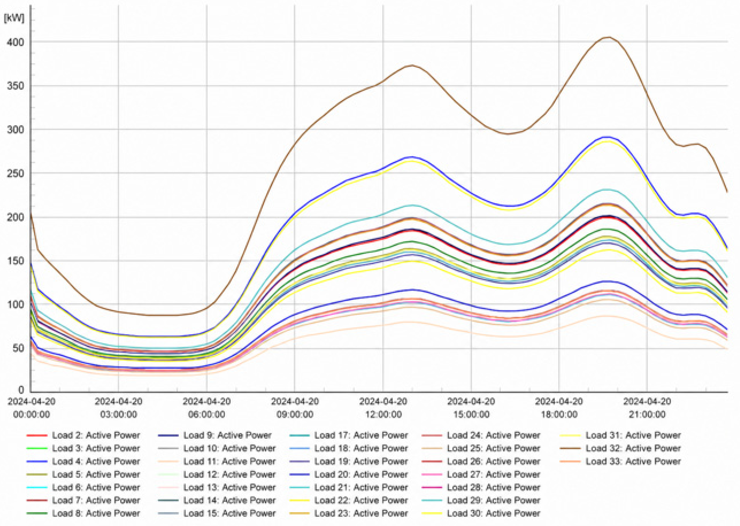
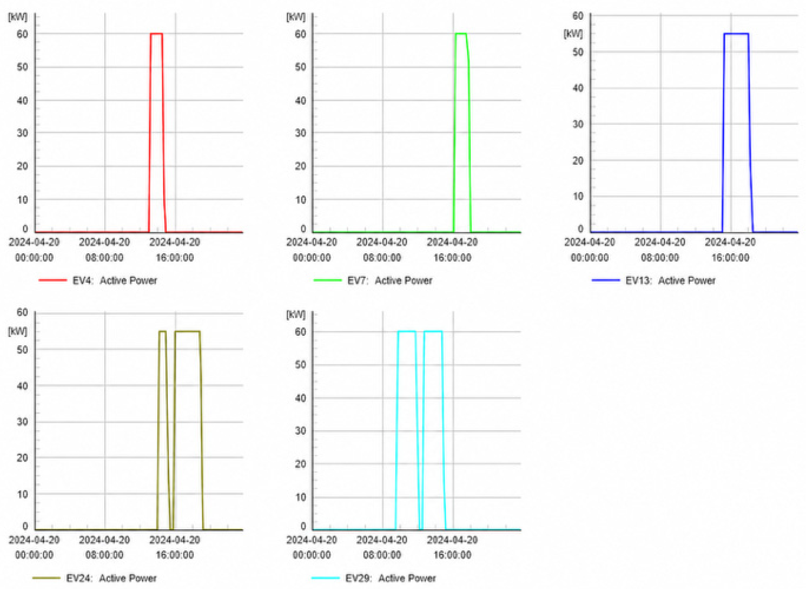
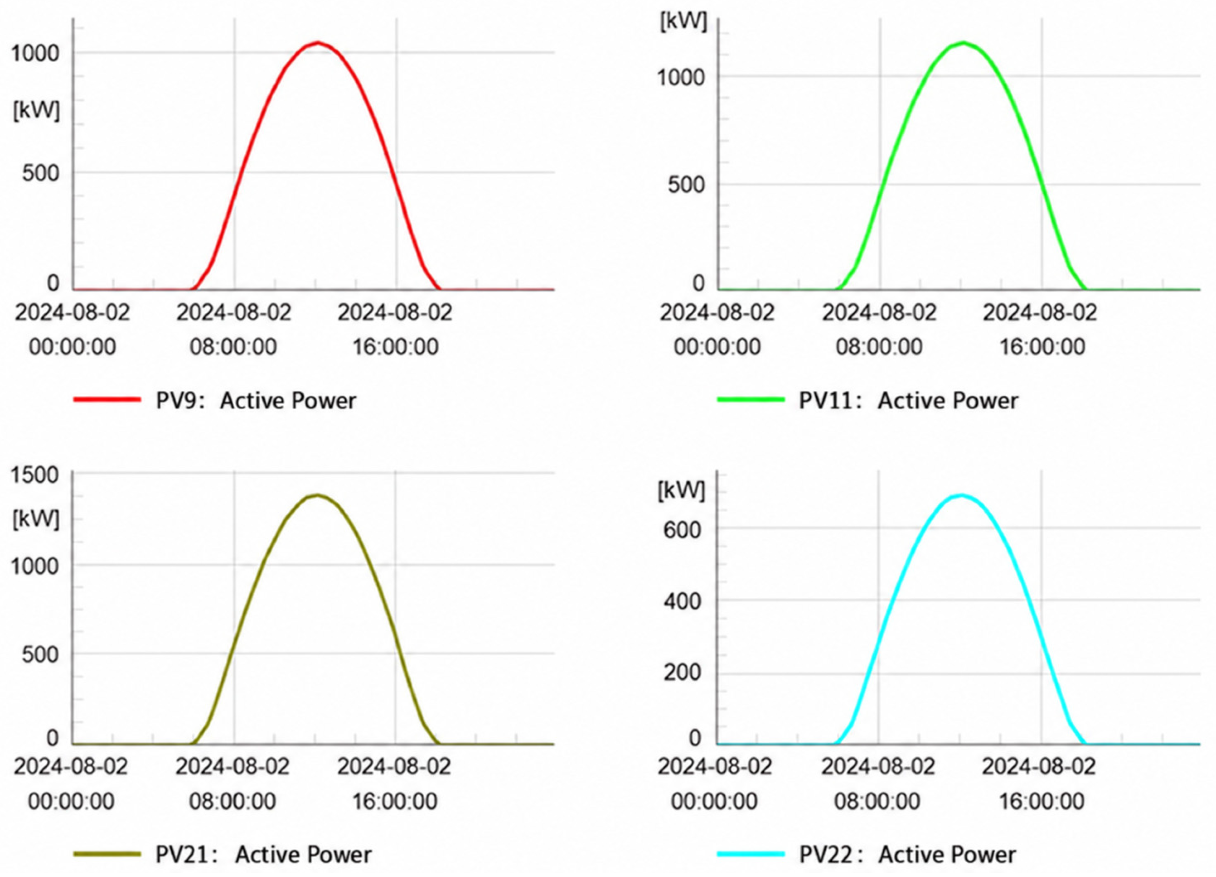
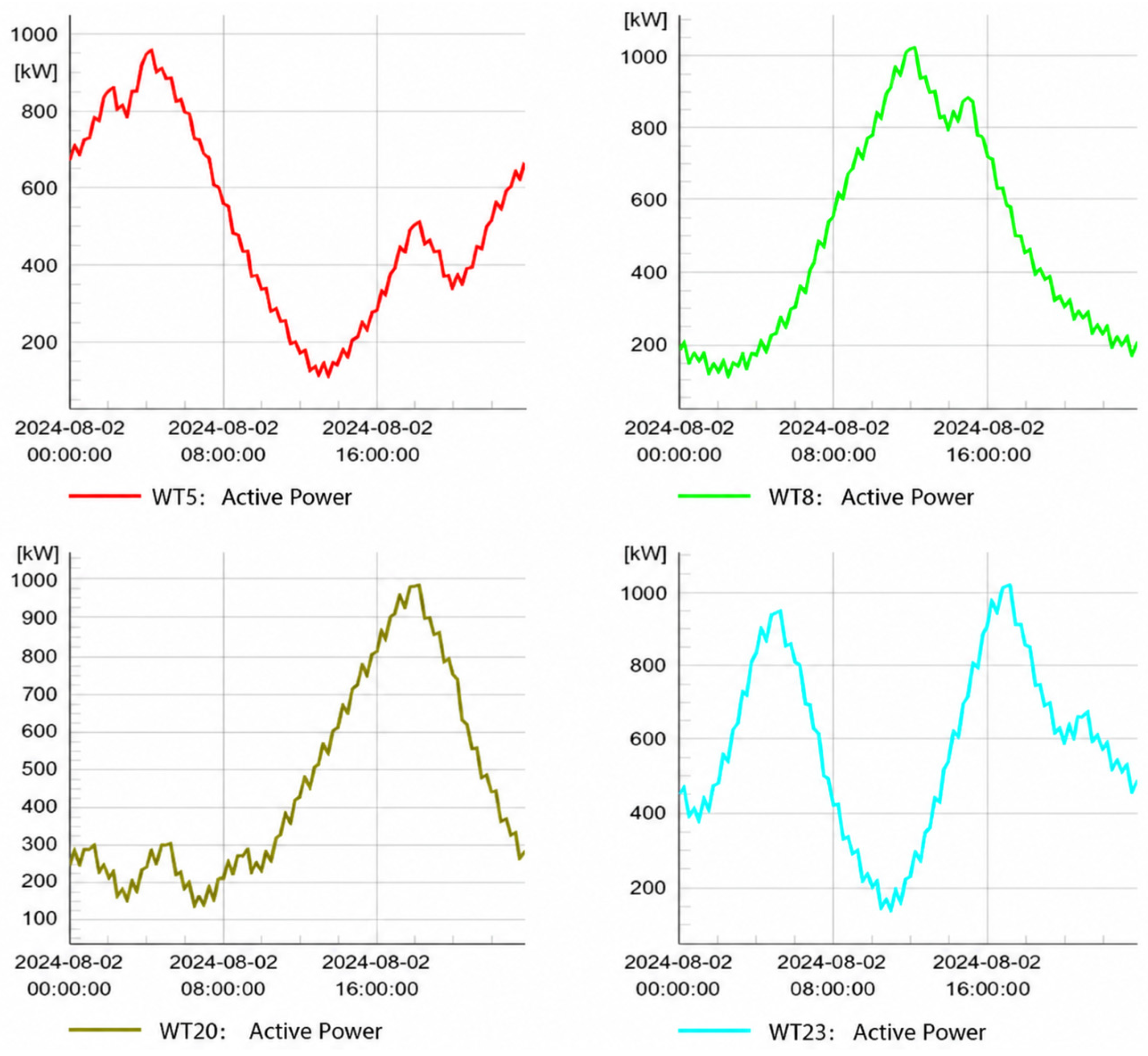
Connected entities affect the shape of a node’s daily active-power curve through their generation and consumption patterns. Here, a temporal signature denotes the curve morphology associated with these patterns, including peak timing and duration, slopes, valley levels, and local fluctuations. Figure 1, Figure 2, Figure 3, Figure 4 and Figure 5 illustrate the load, EV-charging, renewable-generation, and mixed profiles used to examine these characteristics.

For a load-only node, the daily active-power curve mainly reflects users’ consumption habits and generally exhibits smooth peak–valley variation, as shown in Figure 1.

Figure 1. Daily active-power curve of a load-only node.

Figure 1. Daily active-power curve of a load-only node.

EV charging adds demand during charging intervals. Concentrated charging activity can therefore produce sustained increases or abrupt local rises in the active-power profile, as illustrated in Figure 2.

Figure 2. Daily active-power demand of EV charging piles.

Figure 2. Daily active-power demand of EV charging piles.

PV generation is concentrated during daylight hours. The output profiles in Figure 3 have a common daytime rise and fall, with different peak magnitudes across the PV units.

Figure 3. Daily active-power outputs of PV units.

Figure 3. Daily active-power outputs of PV units.

Wind-turbine output exhibits variation in peak timing, ramp direction, and local fluctuations. Figure 4 illustrates four daily profiles with distinct temporal shapes.

Figure 4. Daily active-power curve with wind turbines.

Figure 4. Daily active-power curve with wind turbines.

When several entity types share a node, its net active power follows the balance between demand and generation. With consumption taken as positive, this balance is expressed as:

$$P_{net}(t)=P_L(t)+P_{EV}(t)-P_{PV}(t)-P_W(t)$$

(1)

where $P_L\left(t\right)$ and $P_{EV}\left(t\right)$ are the base-load and EV-charging demands, and $P_V\left(t\right)$ and $P_W\left(t\right)$ are the PV and wind-generation magnitudes, respectively.

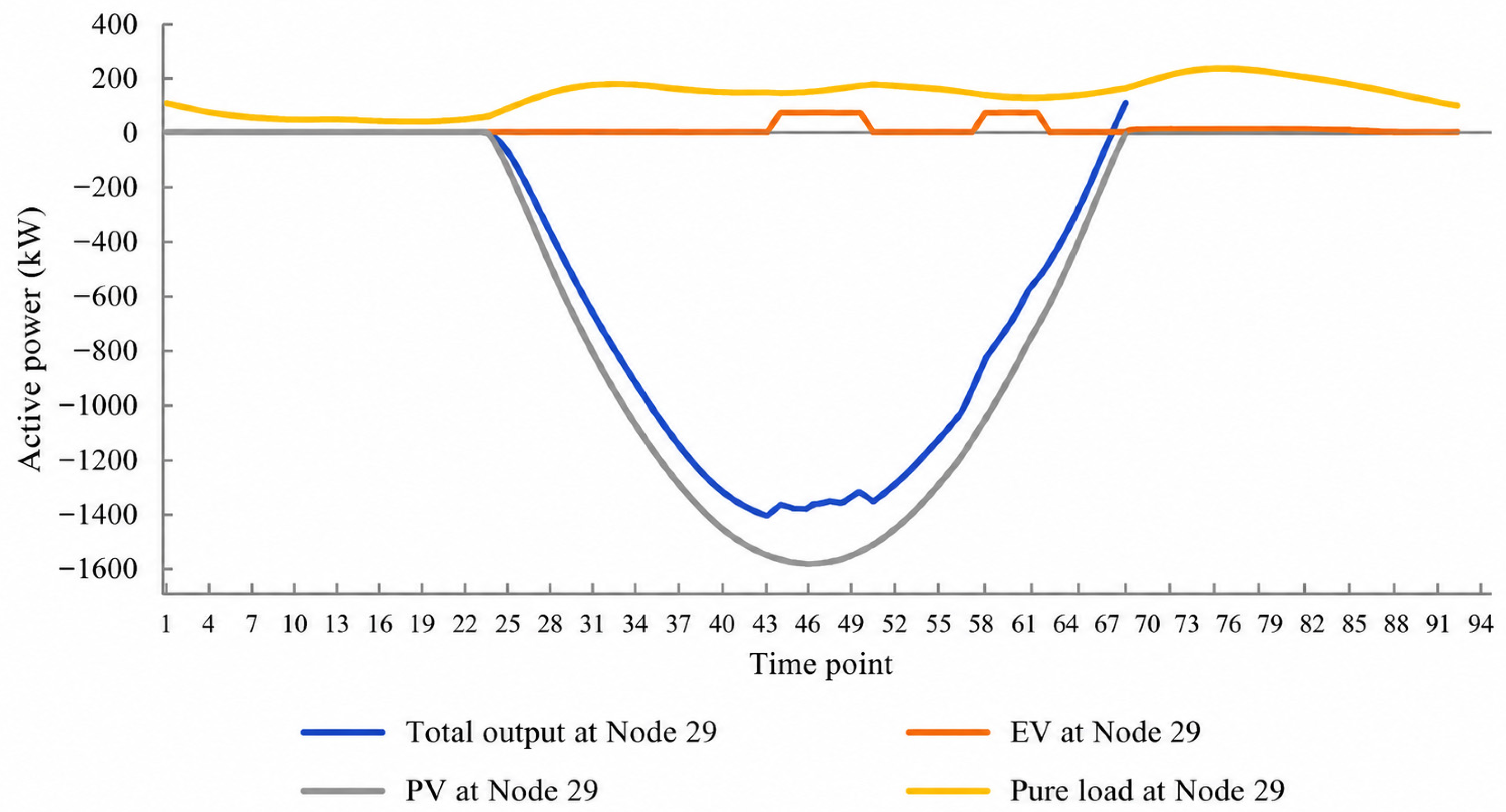
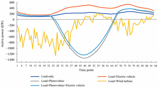
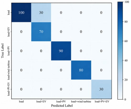
Figure 5 illustrates this balance for the load–PV–EV combination at Node 29, where the wind contribution is zero. The PV contribution is plotted below zero, while the load and EV-charging contributions are positive. Daytime PV generation lowers the net curve and produces net export when it exceeds local demand; charging demand offsets part of this reduction. The total curve thus retains features of both generation and consumption.

Figure 5. Daily net active power and load, PV, and EV-charging contributions at Node 29.

Figure 5. Daily net active power and load, PV, and EV-charging contributions at Node 29.

2.2. Simulation-Based Dataset Construction

The simulation model is based on the IEEE 33-bus radial feeder [14], comprising 33 feeder buses at 12.66 kV, 32 feeder lines, and an upstream 110 kV supply bus, with a nominal frequency of 50 Hz. The five scenarios use the connection locations: four nodes for the load–EV class, six for load–PV, six for load–wind, and Node 29 for the load–PV–EV class. PV, EV, and wind elements are enabled according to the scenario being simulated. Wind generation is represented by doubly fed induction-generator elements whose active-power schedules are specified through relative time characteristics.

For each scenario, quasi-dynamic AC power-flow calculations are performed over 24 h with a 15 min interval. The 96 active-power values measured at a monitored node form one daily sample, and the connected-entity combination determines its class label. These net-power curves are exported to Excel for classification. The dataset contains 2120 samples across five classes; Table 1 summarizes the simulation and sampling settings.

Table 1. Key simulation and dataset settings.

Item	Setting
Simulation platform	PowerFactory
Network prototype	Standard IEEE 33-node radial distribution network
Simulation type	Quasi-dynamic AC simulation
Sampling interval	15 min
Points per node per day	96
Output format	Excel files
Study object	Daily nodal active-power curve

Let sample $i$ be represented by:

$$X_i=[P_{i,1},P_{i,2},\dots ,P_{i,96}]$$

(2)

where $P_{i,t}$ is the active-power value of the sample at time step $t$. The corresponding class label is denoted by $y_i$, where $y_i$∈ {0,1,2,3,4}. The label mapping is provided in Table 2.

Table 2. Five scenarios and their label assignments.

Label	Scenario Class	Typical Connection Characteristic
0	Load-only node	Base load only
1	Load + EV charging piles	Sustained load increase at night and in the evening
2	Load + PV	Influence of PV output during the middle of the day
3	Load + wind turbines	Variable peaks, ramps, and local fluctuations
4	Load + PV + EV charging piles	Combined multi-entity characteristics during daytime and nighttime

3. TabICL-Based Intelligent Identification Model for Grid-Connected Entities Under Limited Measurement Scenarios

3.1. Overall Framework of the TabICL-Based Identification Method

TabICL is a pretrained foundation model for tabular classification [13]. It learns reusable representations from synthetic tabular tasks and uses labeled samples from a new task as context for prediction. In this study, the context consists of daily active-power curves and their connected-entity labels.

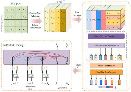
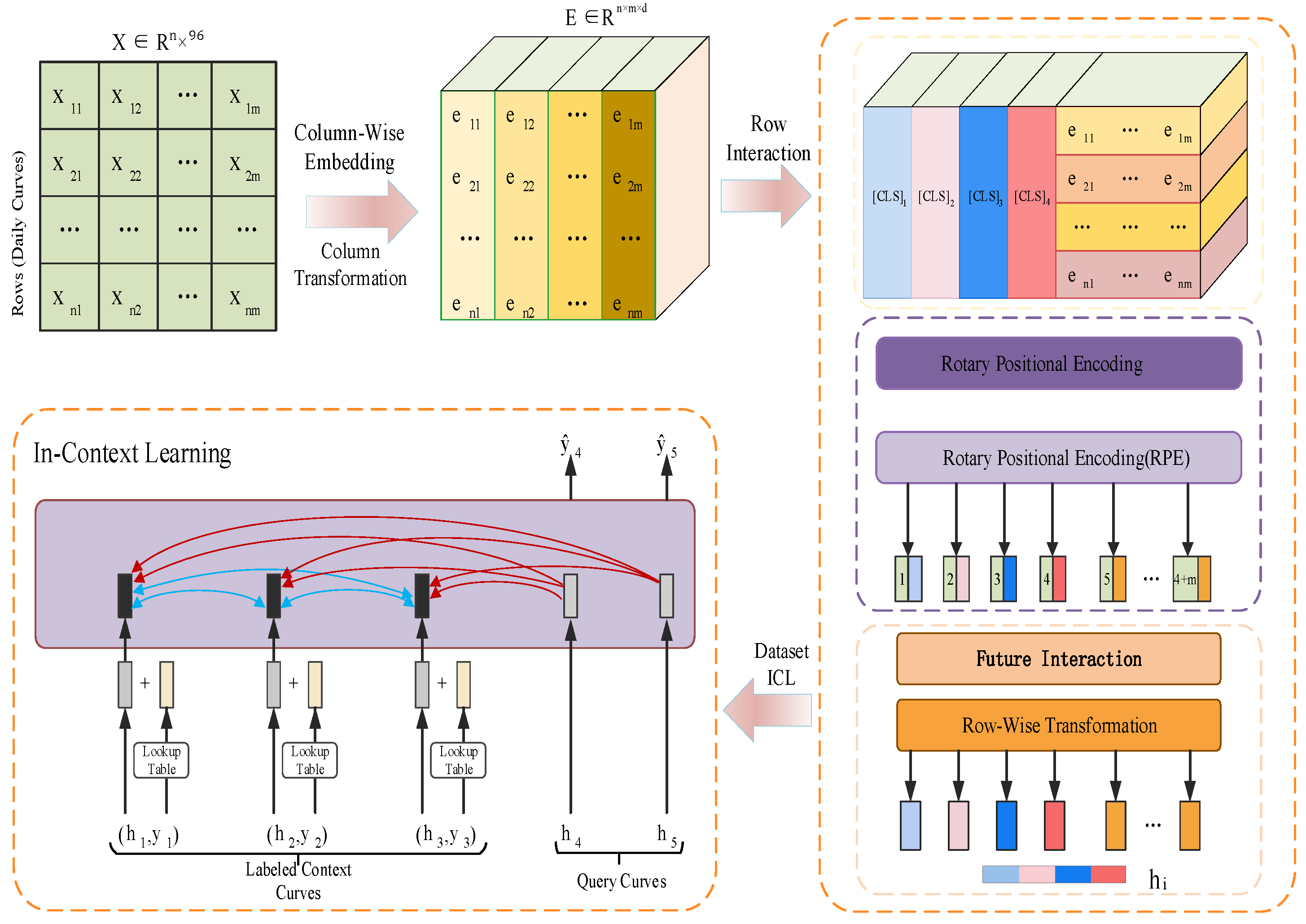
Figure 6 links the TabICL architecture [13] to the five-class identification task. The input table X has n daily curves and m = 96 time-point columns. Column-wise distribution-aware embedding maps the input cells into a tensor E of dimensions n × m × d, where d is the embedding dimension. Row-wise feature interaction then combines the 96 cell embeddings into a representation of each daily curve. At the dataset level, the representations of labeled context curves are combined with their class embeddings to infer the class probabilities of query curves. The class with the highest probability is the identification output.

Figure 6. TabICL architecture adapted to the five-class grid-connected-entity identification task.

3.2. Column-Wise Distribution-Aware Embedding

Before row-wise feature interaction, TabICL first applies column-wise distribution-aware embedding to the input table. Let cj denote the set of samples in column j, containing the power values of all samples at the same time instant. The model treats the column as an unordered set and uses a shared Set Transformer to extract its overall distributional information, from which the corresponding weight $W$ and bias $B$ are generated [15]:

$$W,B=T{F}_{col}(c_j)\in R^{n\times d}$$

(3)

After the column-level parameters are obtained, the embedding of each cell can be written as:

$$e_j=W\odot c_j+B\in R^{n\times d}$$

(4)

where $T{F}_{col}\left(··\right)$ denotes the column-feature extraction module, n is the number of samples, d is the embedding dimension, ⊙ denotes element-wise multiplication, and e_j is the embedding result of column j. Thus, a cell representation contains not only the original power value, but also the overall statistical information of the column corresponding to that time instant. The subsequent model can therefore make decisions using both local values and column-distribution characteristics.

In implementation, the shared Set Transformer first uses a linear mapping to unify the feature dimensions. It then encodes the within-column sample set using induced self-attention; the core computation can be expressed as follows:

$$U=Lin(c)$$

(5)

$$M=MA{B}_1(V_I,U_{train},U_{train})$$

(6)

$$V=MA{B}_2(U,M,M)$$

(7)

$$W,B=Lin(V)$$

(8)

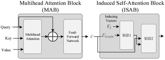
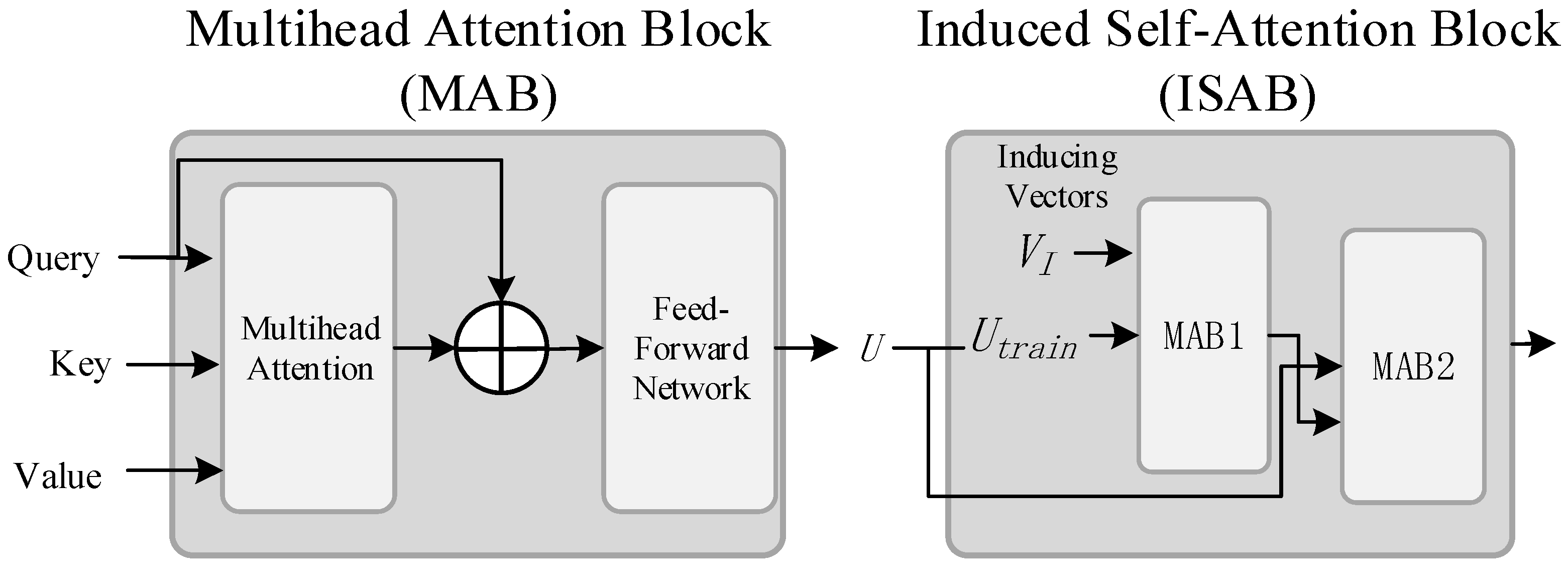
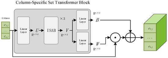
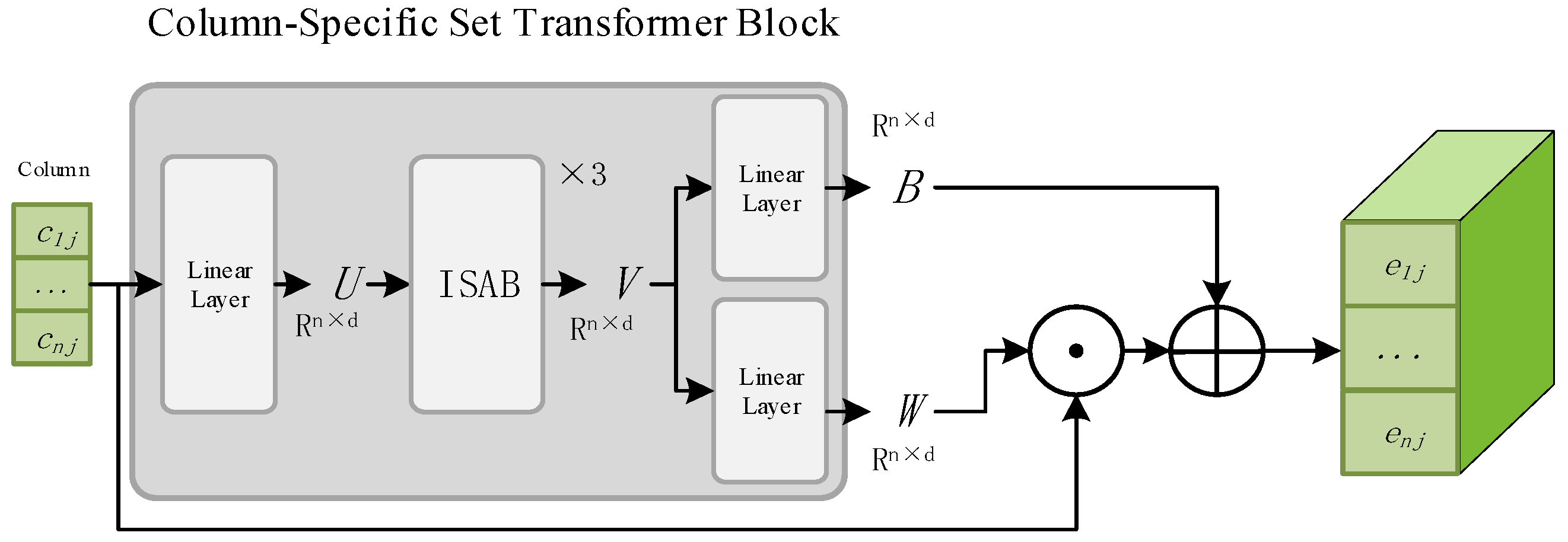
where $Lin\left(··\right)$ denotes the linear mapping, $MAB$ denotes the multihead attention block, $V_I$ denotes the inducing vector, and $U_{train}$ denotes the list of training samples. $MAB$ is the fundamental computational unit of the Set Transformer and performs attention aggregation among queries, keys, and values. Figure 7 presents the architectures of $MAB$ and ISAB, and Figure 8 illustrates how the shared Set Transformer generates column weights and biases and subsequently forms column embeddings. In other words, rather than treating an instantaneous power value in isolation, the model first captures the distributional properties of that time instant across all samples and then maps those properties into the corresponding cell representation.

Figure 7. Architectures of MAB and ISAB.

Figure 8. Column embeddings generated by the shared Set Transformer.

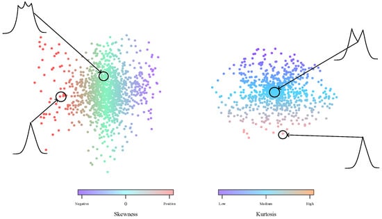
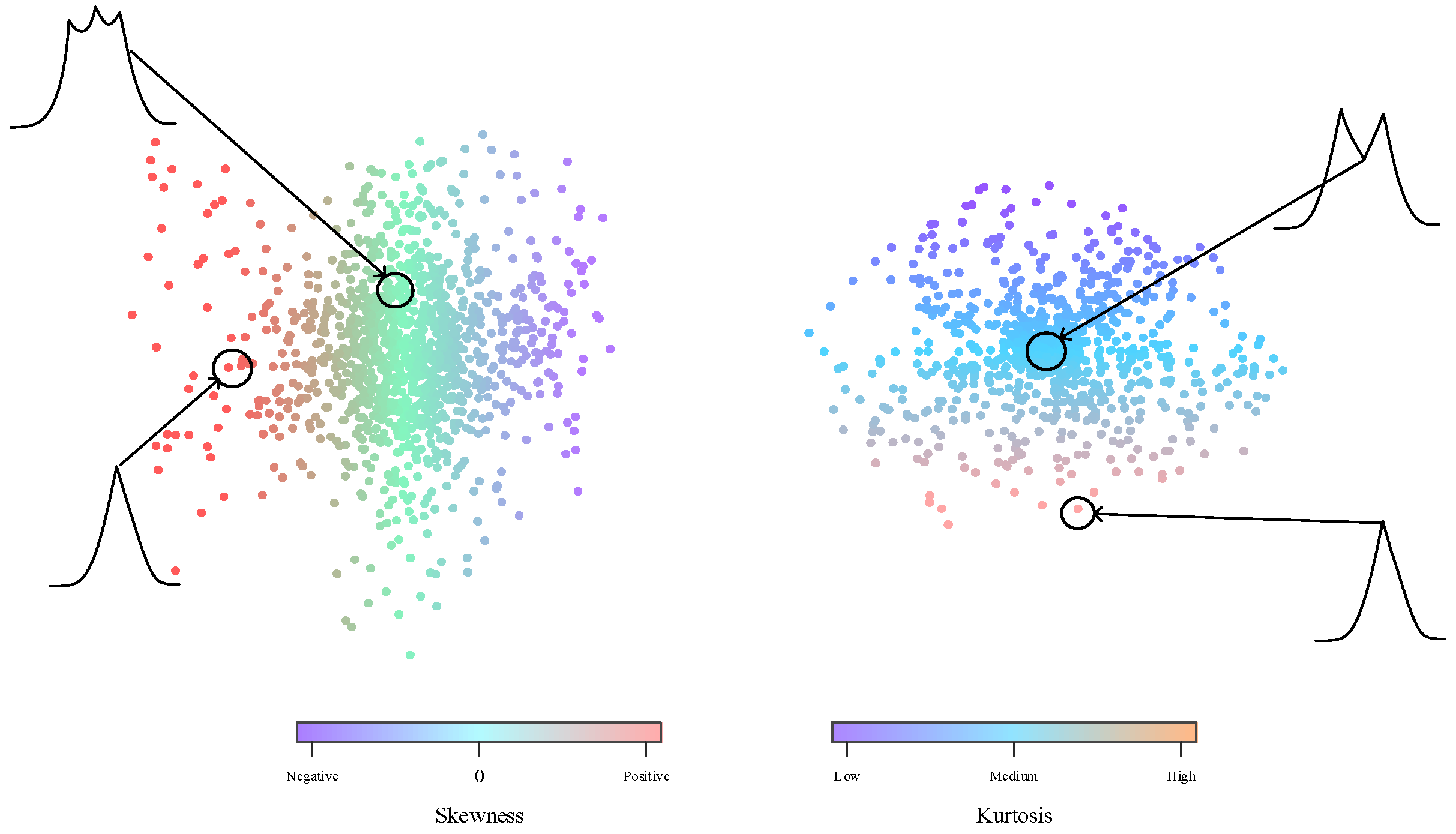
Figure 9 illustrates the distribution-sensitive character of the column embeddings [13]. In the two-dimensional projections, columns are colored by skewness and kurtosis, and columns with similar statistics tend to occupy nearby regions. For the daily-curve representation used here, this mechanism provides a way to distinguish time-point columns with different power-value distributions before row-wise interaction.

Figure 9. Distribution of column embeddings organized by skewness and kurtosis.

3.3. Row-Wise Feature Interaction and Rotary Positional Encoding

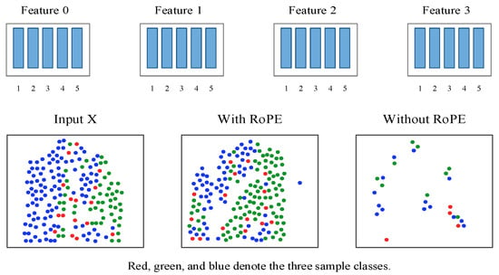
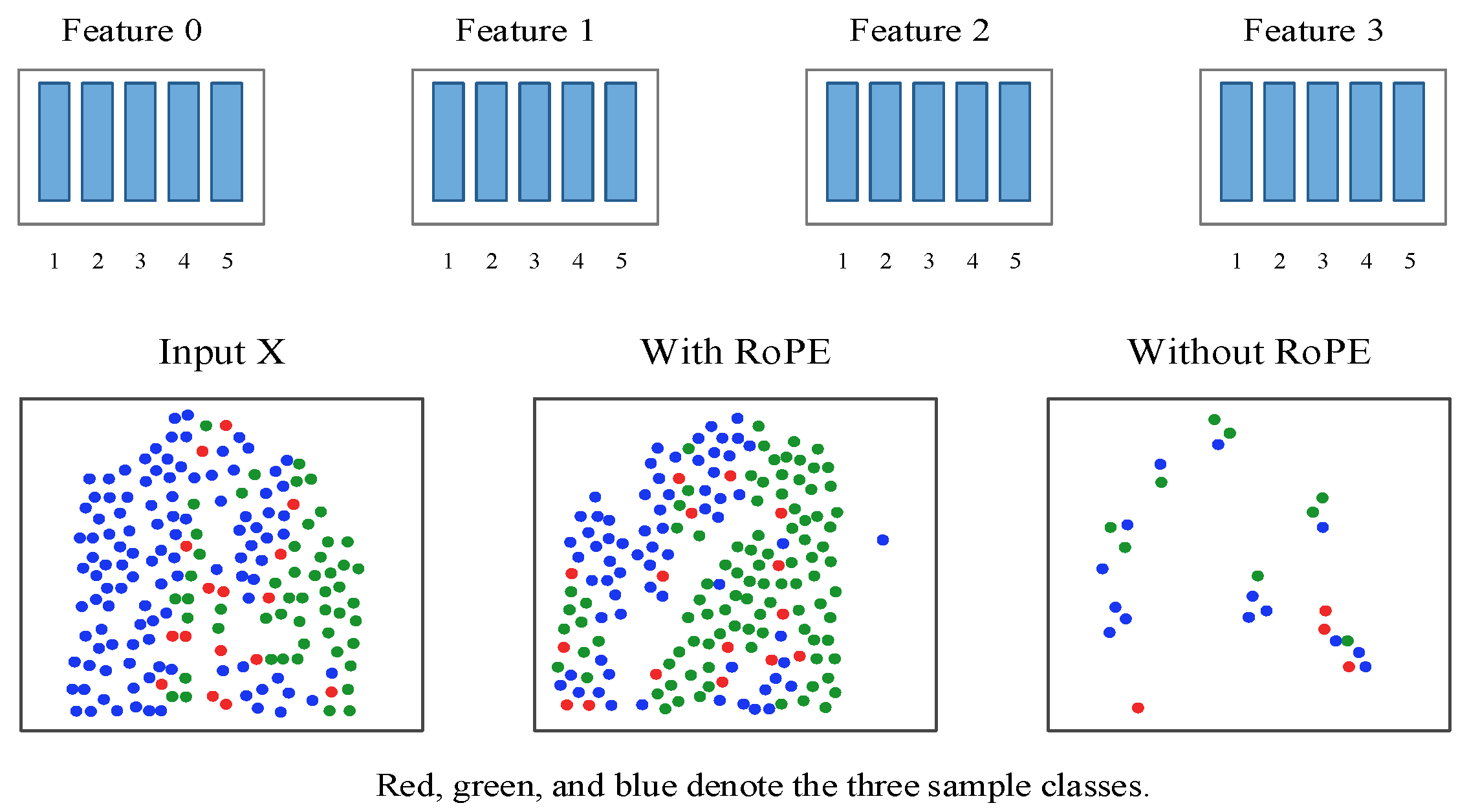
The row-wise module models interactions among the time-point features of each daily curve. Learnable [CLS] tokens are prepended to the cell embeddings, and their Transformer outputs [16] are concatenated to form the row representation H. Rotary positional encoding (RoPE) distinguishes feature positions during this interaction. The 96 columns are retained in chronological order in the present application. Figure 10 illustrates how RoPE helps preserve separability when features have similar marginal distributions [13]: the representations obtained with RoPE retain the sample structure more clearly than those obtained without it.

Figure 10. RoPE suppressing representation collapse toward an identical distribution.

After the feature representation of each sample is obtained, TabICL jointly evaluates the known-class samples in the training set and the test sample. Let the training set be $D_{train}=\left\{\left.\left(x_i,y_i\right)\right\}\right.$ and the test sample be $x_{test}$; the final classification probability can then be expressed as follows:

$$p(\cdot |x_{test},D_{train})=T{F}_{icl}(H_{train},H_{test})$$

(9)

where $x_{test}$ denotes the test sample to be identified, $D_{train}$ denotes the support set composed of labeled training samples, and $p(\cdot |x_{test},D_{train})$ denotes the class-probability distribution conditioned on the test sample and support set. $T{F}_{icl}\left(··\right)$ denotes the in-context learning mapping function of TabICL, while $H_{train}$ and $H_{test}$ denote the serialized input representations of the training support set and test sample, respectively. The model assigns the class corresponding to the maximum value in this probability distribution as the final prediction.

4. Experimental Design and Results

4.1. Experimental Dataset

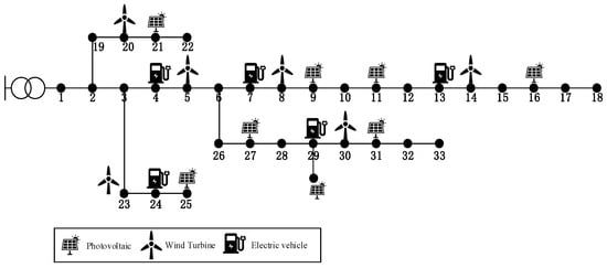
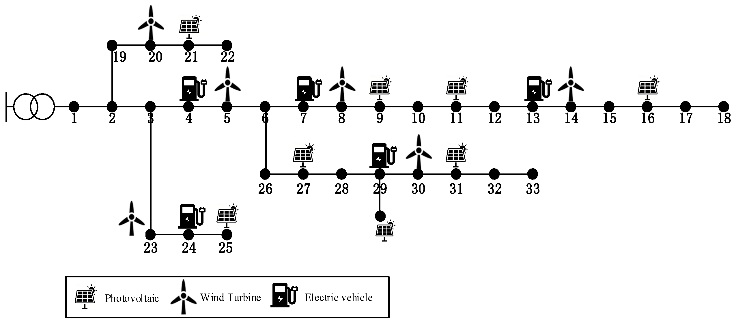
Figure 11 illustrates the topology of the IEEE 33-node distribution network and the connection locations of the grid-connected entities considered in this study.

Figure 11. IEEE 33-node distribution-network topology and connection locations of grid-connected entities.

The connection relationships and class distribution of the five IEEE 33-node scenarios are listed in Table 3.

Table 3. Connection locations and sample distribution of the five scenarios.

Scenario Class	Connection Nodes	Total	Training	Test
Load-only node	2, 6, 10, 12, 15, 17, 18, 26, 28, 32	600	470	130
Load + EV charging piles	4, 7, 13, 24	400	330	70
Load + PV	9, 16, 21, 25, 27, 31	540	450	90
Load + wind turbines	5, 8, 14, 20, 23, 30	480	400	80
Load + PV + EV charging piles	29	100	70	30

The dataset contains 2120 daily samples, of which 1720 form the training set and 400 form the test set. Table 3 lists the connection nodes, class sizes, and allocation of each class. The original class distribution is retained without minority-class augmentation. All classifiers use these same training and test samples.

Figure 12 compares the mean daily curves of the five classes. Their different demand and generation patterns provide an initial basis for classification. The means summarize class-level behavior, while individual curves can overlap; a high evening peak at a load-only node, for example, can resemble additional EV-charging demand.

Figure 12. Comparison of the mean daily curve profiles for the five classes.

4.2. Analysis of Identification Results for New Grid-Connected Entities

Accuracy, precision, recall, F1 score, macro-averaged F1 score, and the confusion matrix were used to evaluate five-class identification performance.

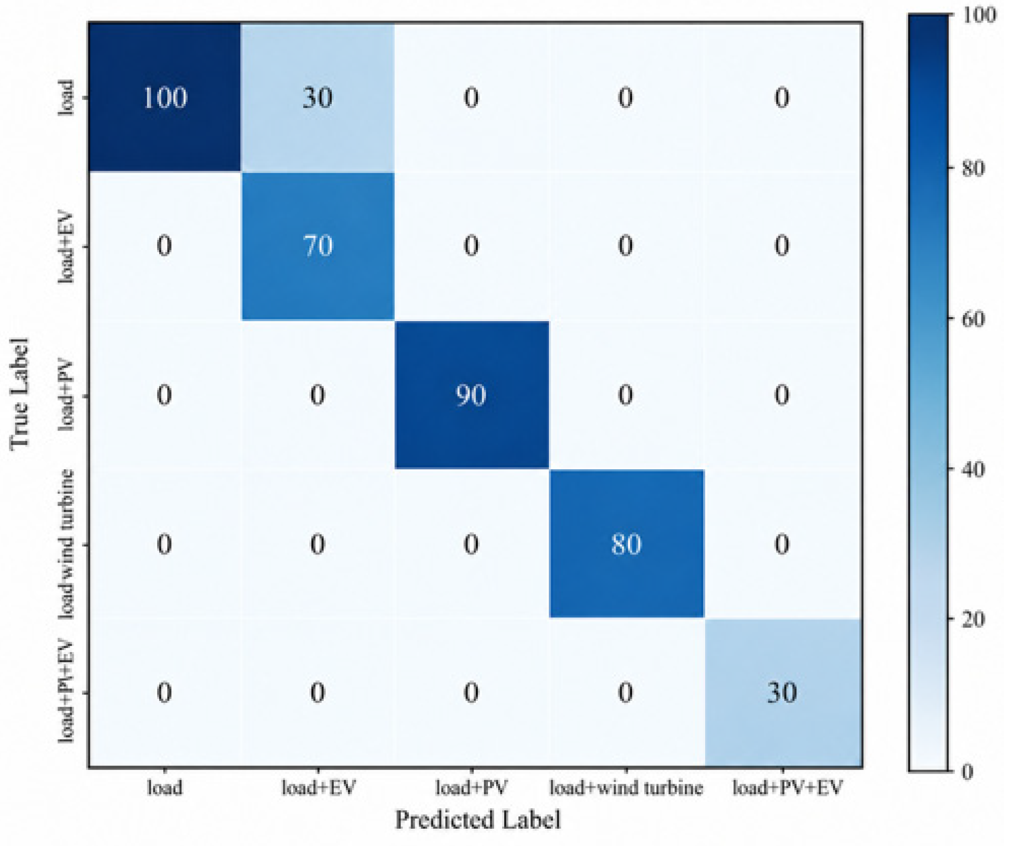
The simulation-based test results show that TabICL achieved an overall accuracy of 92.50% and a macro-averaged F1 score of 0.9386, with 30 out of the 400 test samples misclassified, corresponding to an error rate of 7.50%. These results indicate that by retaining the complete sequence of 96 sampling points, the model can exploit the temporal characteristics of daily active-power curves, including evening peaks, midday generation patterns, and short-term fluctuations. The detailed data are presented in Table 4.

Table 4. Classification performance on the simulation-based test set.

Class	Precision	Recall	F1 Score	Samples
Load-only node	1.0000	0.7692	0.8696	130
Load + EV charging piles	0.7000	1.0000	0.8235	70
Load + PV	1.0000	1.0000	1.0000	90
Load + wind turbines	1.0000	1.0000	1.0000	80
Load + PV + EV charging piles	1.0000	1.0000	1.0000	30
Macro average	0.9400	0.9538	0.9386	400
Weighted average	0.9475	0.9250	0.9267	400

Table 4 shows that the load–PV, load–wind, and load–PV–EV classes each achieved precision, recall, and F1 scores of 1.0000 on the simulation test set. Their daytime generation patterns and wind-power variations provide distinct temporal signatures in this dataset. The remaining errors were concentrated at the boundary between the load-only and load–EV curves.

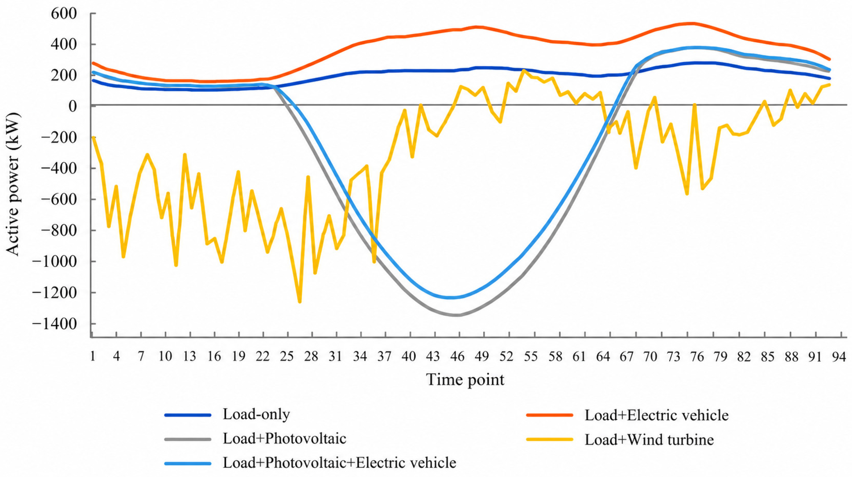
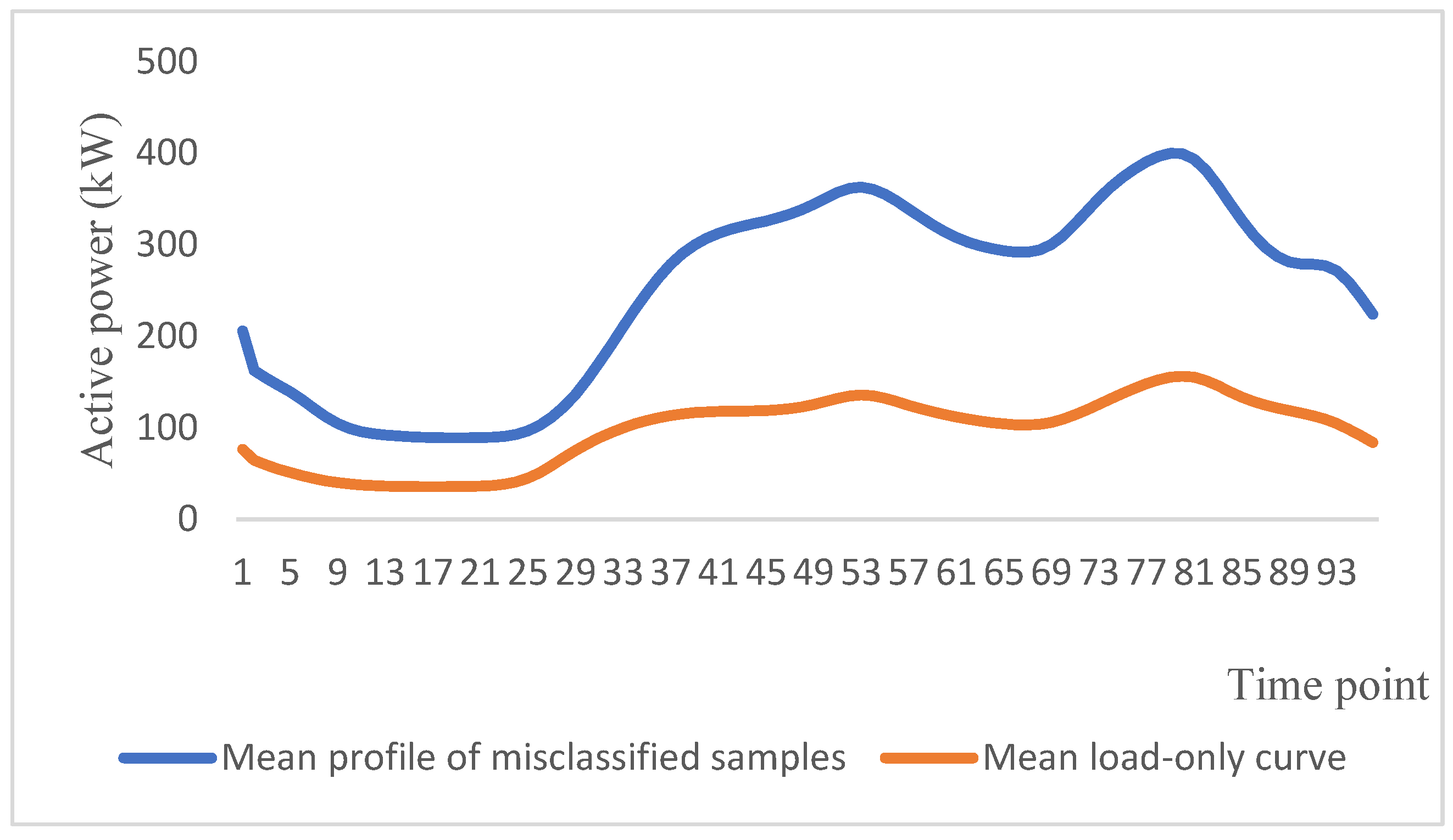
The confusion matrix in Figure 13 shows that all errors occurred between the load-only and load-plus-EV-charging-pile classes. Specifically, 100 out of the 130 load-only samples were identified correctly, while the remaining 30 were misclassified as load-plus-EV charging piles, giving the load-only class a recall of 0.7692. All 70 true load-plus-EV-charging-pile samples were correctly recalled, but the 30 false positives from the load-only class reduced its precision to 0.7000. In contrast, all 200 samples in the load-plus-PV, load-plus-wind-turbine, and load-plus-PV-and-EV-charging-pile classes were classified correctly. Thus, the observed error was localized to a specific class boundary rather than distributed across all five classes. The 30 misclassified curves came from the same load-only node; their pronounced evening power increase resembled an EV-charging profile, and reliance on active power alone made this boundary more difficult to resolve.

Figure 13. Confusion matrix on the simulation-based test set.

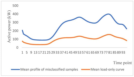
Figure 14 compares the mean profile of the misclassified samples with the mean load-only curve. The stronger evening increase in the misclassified group resembles the additional demand caused by EV charging, explaining the overlap at this class boundary. Peak timing, magnitude, and duration therefore remain important features for improving discrimination between these two scenarios.

Figure 14. Comparison of the mean profile of misclassified samples with the mean load-only curve.

4.3. Direct Comparison with Baseline Models

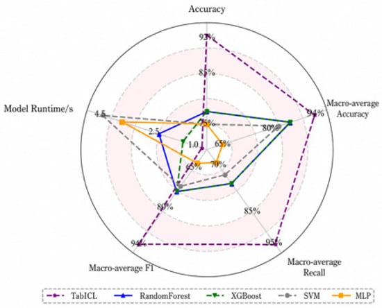
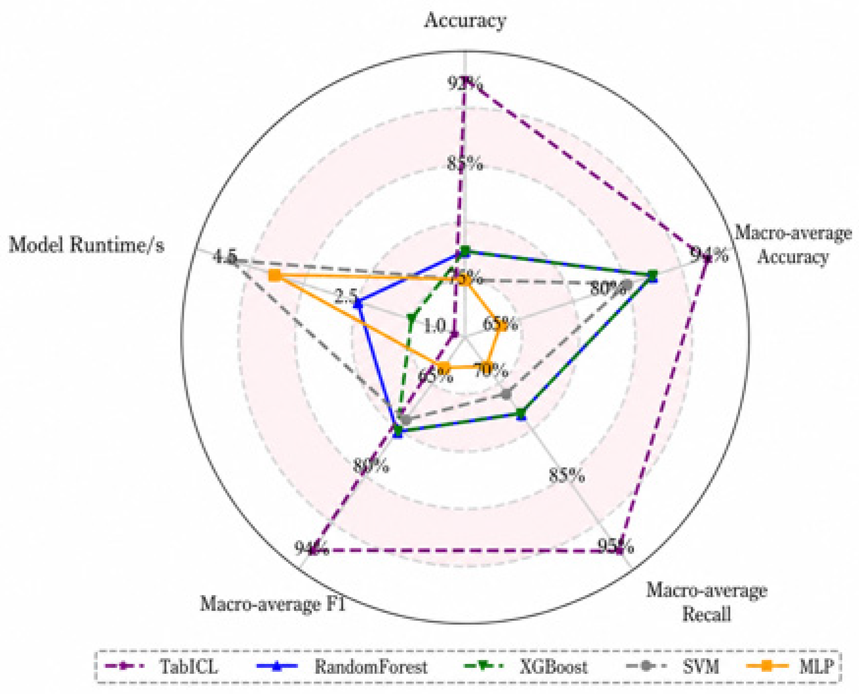
To make the performance comparison explicit, SVM [17], random forest [18], XGBoost [19], and MLP [20] were selected as baseline models. All five methods used the same 1720 training samples, the same 400 test samples, the same 96-point active-power inputs, and the same evaluation metrics; runtime was measured in the same experimental environment. The SVM used a radial-basis-function kernel, random forest comprised 400 decision trees, XGBoost used 300 boosting rounds, and the MLP had two hidden layers. As shown in Table 5, TabICL achieved an accuracy of 0.9250, which was 0.1500 (15.00 percentage points) higher than random forest and XGBoost and 0.1750 (17.50 percentage points) higher than SVM and MLP. Its macro-averaged F1 score of 0.9386 exceeded those of random forest and XGBoost by 0.1990, SVM by 0.2186, and MLP by 0.3075. TabICL also had the shortest reported runtime at 0.69 s compared with 1.40–4.43 s for the baselines. These direct differences show that the proposed approach provides the strongest clean-data classification performance among the evaluated methods under the reported experimental conditions.

Table 5. Overall performance comparison of different models.

Model	Accuracy	Macro-Precision	Macro-Recall	Macro-F1	Time (s)
TabICL	0.9250	0.9400	0.9538	0.9386	0.69
Random Forest	0.7750	0.8636	0.7590	0.7396	2.30
XGBoost	0.7750	0.8636	0.7590	0.7396	1.40
SVM	0.7500	0.8274	0.7304	0.7200	4.43
MLP	0.7500	0.6500	0.6923	0.6311	3.70

TabICL provided the highest clean-data accuracy and the shortest measured runtime among the evaluated models. Figure 15 summarizes the performance measures. Its noise-robustness axis uses the mean accuracy across the 40, 30, and 20 dB conditions examined in Section 4.4, allowing the clean-data advantage to be considered alongside sensitivity to measurement noise.

Figure 15. Radar chart comparing the overall performance of different models.

4.4. Noise Robustness Analysis

Noise robustness was evaluated by adding white Gaussian noise to the test curves at SNRs of 40, 30, and 20 dB, following the evaluation approaches in Refs. [21,22]. The signal-to-noise ratio is defined as:

$$SNR=10lg({\displaystyle \frac{P_s}{P_n}})$$

(10)

where $P_s$ and $P_n$ denote the original signal power and the added noise power, respectively, and $SNR$ is expressed in dB. Each noise condition is repeated 20 times, and mean accuracy is used to compare the classifiers.

Table 6 reports the mean accuracy under the three noise conditions. Relative to its noise-free accuracy of 0.9250, TabICL achieved 0.8888 at 40 dB, a decrease of 3.62 percentage points. Its accuracy fell to 0.5575 at 30 dB and 0.6062 at 20 dB, corresponding to decreases of 36.75 and 31.88 percentage points. At 40 dB, TabICL exceeded random forest and XGBoost by 0.1138 and SVM and MLP by 0.1388. At 30 and 20 dB, all four baselines achieved higher accuracy, indicating that TabICL’s clean-data advantage is accompanied by greater sensitivity to strong noise.

Table 6. Accuracy comparison of different models under various SNR conditions.

Model	Noise-Free	40 dB	30 dB	20 dB
TabICL	0.9250	0.8888	0.5575	0.6062
Random Forest	0.7750	0.7750	0.7750	0.7700
XGBoost	0.7750	0.7750	0.7675	0.7550
SVM	0.7500	0.7500	0.7512	0.7638
MLP	0.7500	0.7500	0.7500	0.7488

It is noteworthy that TabICL achieved slightly higher accuracy at 20 dB than at 30 dB, so the results do not show a strictly monotonic decline. This difference does not imply that stronger noise improves performance. With the small test set, noise at different intensities may perturb individual boundary samples in different directions. Although the signals were noisier overall at 20 dB, the perturbation may have slightly increased the separation between the two classes for some boundary samples. The overall trend is therefore more informative: under strong noise, TabICL performs substantially worse than under noise-free and low-noise conditions.

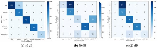
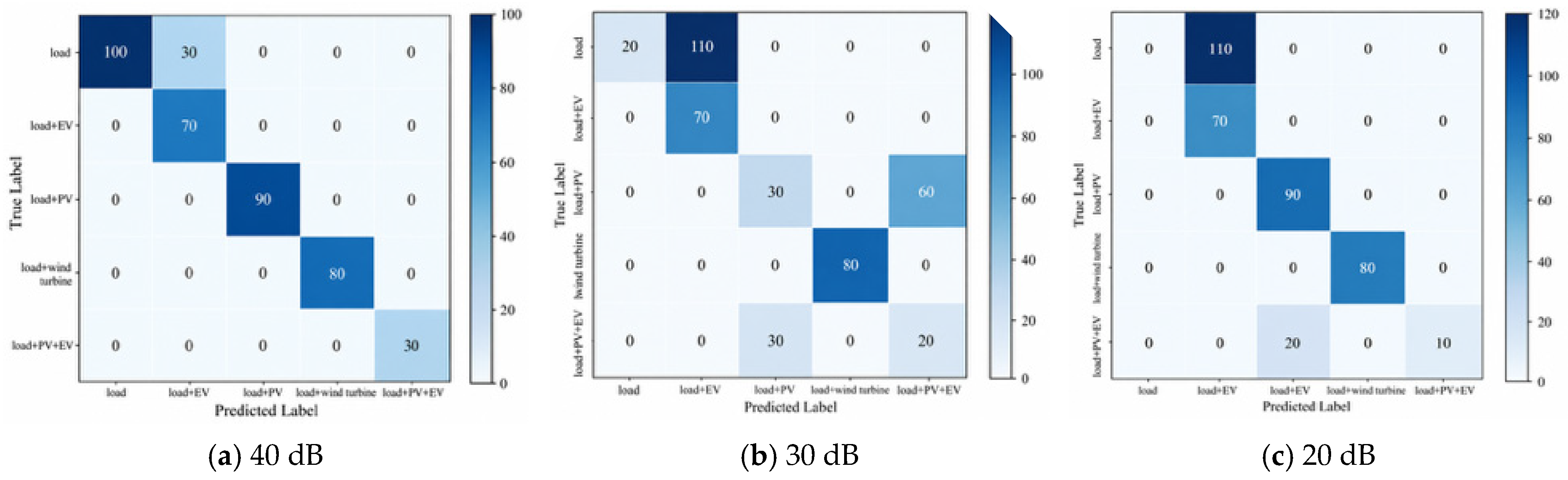
Panels (a), (b), and (c) in Figure 16 present the confusion matrices at SNRs of 40, 30, and 20 dB, respectively. The test conditions for all three experiments were identical to those in Table 6, and the matrices were plotted from predictions obtained after random noise injection.

Figure 16. Representative confusion matrices of TabICL at 40, 30, and 20 dB.

Under low-level noise at 40 dB, only a subset of load-only samples was misclassified as load-plus-EV charging piles, indicating that the boundary between these two classes was the most vulnerable. At 30 dB, these errors increased, and load-plus-PV samples were also more likely to be misclassified as load-plus-PV and EV charging piles. Under strong noise at 20 dB, all load-only samples were misclassified as EV charging piles, and confusion between the PV and hybrid classes intensified. The wind-turbine and EV-charging-pile characteristics were comparatively resistant to interference.

5. Conclusions and Future Work

5.1. Conclusions

This study developed a TabICL-based method for classifying connected-entity combinations from a single 96-point daily nodal active-power curve. The method combines column-wise distribution-aware embedding, row-wise feature interaction, and in-context learning to distinguish five scenarios in an IEEE 33-bus simulation dataset. On the common 400-sample test set, it achieved 92.50% accuracy and a macro-averaged F1 score of 0.9386, exceeding the four baselines by 15.00–17.50 percentage points in accuracy. The remaining errors occurred between load-only and load–EV curves with similar evening demand patterns. Accuracy remained 0.8888 at 40 dB but fell to 0.5575 and 0.6062 at 30 and 20 dB, identifying strong-noise robustness as a main limitation. The experiments establish feasibility on the modeled 12.66 kV radial feeder; extension to operating low-voltage networks requires validation across feeder conditions, equipment behavior, and measurement quality.

5.2. Future Work

Future research will focus on four directions that address the limitations of the present simulation-based study.

(1) Improve the robustness of the identification algorithm. The current results show that its performance deteriorates under strong noise. Future work will develop disturbance-aware data-processing and learning strategies so that the classifier can maintain stable identification when measurements contain noise, missing values, outliers, or other data-quality problems encountered in practice.

(2) Improve identification accuracy through multi-source information fusion. Future studies will combine complementary electrical measurements with spatial information from neighboring nodes so that the model can describe entity behavior from multiple perspectives. The objective is to reduce the remaining overlap between classes with similar daily patterns, particularly load-only and EV-charging profiles, and to improve identification under complex operating conditions.

(3) Enhance the generalization ability of the method. Future training and validation data will cover different feeders, seasons, day types, load levels, renewable-energy penetration levels, and connection locations. Field measurements with verified equipment labels will be incorporated when available, and cross-domain learning will be investigated to reduce the difference between simulated and real data. The aim is to maintain stable identification performance when the network or operating condition changes.

(4) Evaluate practical deployment. Future studies will measure computing-resource use and response time on distribution-network monitoring terminals to determine whether the method can support routine identification. Confidence-based decisions will also be investigated so that uncertain samples can be submitted for verification. The objective is dependable identification within the operating constraints of practical monitoring systems.

References

- Zhang, S.; Wang, W.; Qian, Y.; Zhao, X.; Du, L.; Zhang, W. Research progress of non-intrusive load monitoring for deep learning. Comput. Syst. Appl. 2023, 32, 25–47. (In Chinese) [Google Scholar]
- Wang, H.; Chen, Y.; Li, G.; Zhang, S.; Wang, W.; Qian, Y.; Zhao, X.; Du, L.; Zhang, W. Solution to voltage violations in distribution networks with large-scale distributed photovoltaic integration. J. Northeast Electr. Power Univ. 2017, 37, 8–14. (In Chinese) [Google Scholar]
- Zhang, S.; Wang, W.; Qian, Y.; Zhao, X.; Du, L.; Zhang, W. Edge-cloud collaborative identification framework for power-quality disturbances based on image analysis. Proc. CSEE 2025, 45, 4593–4607. (In Chinese) [Google Scholar]
- ENTSO-E Expert Panel. Final Report on the Grid Incident in Spain and Portugal on 28 April 2025; European Network of Transmission System Operators for Electricity: Brussels, Belgium, 2026. Available online: https://www.entsoe.eu/publications/blackout/28-april-2025-iberian-blackout/ (accessed on 24 October 2026).
- Tong, W.; Saifuddin, M.R.; Logenthiran, T. Microgrid management encompassing AC and DC renewable generations with energy storages. In Proceedings of the 2018 IEEE Innovative Smart Grid Technologies—Asia (ISGT Asia), Singapore, 22–25 May 2018; pp. 1262–1267. [Google Scholar] [CrossRef] [Scilit]
- Poh, W.Q.T.; Naayagi, R.T. Modelling and integration of a piezoelectric cantilever beam with quasi-Z-source inverter for self-powered dynamic system application. In Proceedings of the 2020 IEEE Power & Energy Society General Meeting (PESGM), Montreal, QC, Canada, 2–6 August 2020; pp. 1–5. [Google Scholar] [CrossRef] [Scilit]
- Srinivas, V.L.; Wu, J. Topology and parameter identification of distribution network using smart meter and micro-PMU measurements. IEEE Trans. Instrum. Meas. 2022, 71, 9004114. [Google Scholar] [CrossRef] [Scilit]
- Zhang, S.; Wang, W.; Qian, Y.; Zhao, X.; Du, L.; Zhang, W. Topology identification technology for low-voltage intelligent distribution networks and improvement measures. Rural Electrif. 2025, 5, 39–43. (In Chinese) [Google Scholar]
- Zhang, S.; Wang, W.; Qian, Y.; Zhao, X.; Du, L.; Zhang, W. Optimal configuration of feeder terminals for topology acquisition in low-voltage distribution areas. Electr. Power 2025, 58, 151–161. (In Chinese) [Google Scholar]
- Hart, G.W. Nonintrusive appliance load monitoring. Proc. IEEE 1992, 80, 1870–1891. [Google Scholar] [CrossRef] [Scilit]
- Kelly, J.; Knottenbelt, W. Neural NILM: Deep neural networks applied to energy disaggregation. In Proceedings of the 2nd ACM International Conference on Embedded Systems for Energy-Efficient Built Environments, Seoul, Republic of Korea, 4–5 November 2015; ACM: New York, NY, USA, 2015; pp. 55–64. [Google Scholar] [CrossRef] [Scilit]
- Zhang, S.; Wang, W.; Qian, Y.; Zhao, X.; Du, L.; Zhang, W. Accurate predictions on small data with a tabular foundation model. Nature 2025, 637, 319–326. [Google Scholar] [CrossRef] [Scilit] [PubMed]
- Qu, J.; Holzmüller, D.; Varoquaux, G.; Le Morvan, M. TabICL: A tabular foundation model for in-context learning on large data. In Proceedings of the 42nd International Conference on Machine Learning, Vancouver, BC, Canada, 13–19 July 2025; Volume 267, pp. 50817–50847. [Google Scholar] [CrossRef] [Scilit]
- Baran, M.E.; Wu, F.F. Network reconfiguration in distribution systems for loss reduction and load balancing. IEEE Trans. Power Deliv. 1989, 4, 1401–1407. [Google Scholar] [CrossRef] [Scilit]
- Lee, J.; Lee, Y.; Kim, J.; Kosiorek, A.; Choi, S.; Teh, Y.W. Set Transformer: A framework for attention-based permutation-invariant neural networks. In Proceedings of the 36th International Conference on Machine Learning, Long Beach, CA, USA, 9–15 June 2019; Volume 97, pp. 3744–3753. [Google Scholar]
- Vaswani, A.; Shazeer, N.; Parmar, N.; Uszkoreit, J.; Jones, L.; Gomez, A.N.; Kaiser, Ł.; Polosukhin, I. Attention is all you need. In Advances in Neural Information Processing Systems 30; Curran Associates, Inc.: Red Hook, NY, USA, 2017; pp. 5998–6008. [Google Scholar]
- Cortes, C.; Vapnik, V. Support-vector networks. Mach. Learn. 1995, 20, 273–297. [Google Scholar] [CrossRef] [Scilit]
- Breiman, L. Random forests. Mach. Learn. 2001, 45, 5–32. [Google Scholar] [CrossRef] [Scilit]
- Chen, T.; Guestrin, C. XGBoost: A scalable tree boosting system. In Proceedings of the 22nd ACM SIGKDD International Conference on Knowledge Discovery and Data Mining, San Francisco, CA, USA, 13–17 August 2016; ACM: New York, NY, USA, 2016; pp. 785–794. [Google Scholar] [CrossRef] [Scilit]
- Hornik, K.; Stinchcombe, M.; White, H. Multilayer feedforward networks are universal approximators. Neural Netw. 1989, 2, 359–366. [Google Scholar] [CrossRef] [Scilit]
- Lin, Z.; Yan, Y.; Liu, Y.; Hu, Y.; Cong, Z.; Feng, L. Early tree-line fault identification method for 10-kV distribution lines based on multi-timescale coupling analysis. Proc. CSEE 2026, 1–17. ahead of print. (In Chinese) [Google Scholar]
- Cheng, J.; Hu, X.; Bao, G.; Meng, J. Composite power-quality disturbance identification based on dual-modal feature fusion and collaborative attention. Sci. Technol. Eng. 2026, 26, 2430–2441. (In Chinese) [Google Scholar]
Disclaimer/Publisher’s Note: The statements, opinions and data contained in all publications are solely those of the individual author(s) and contributor(s) and not of MDPI and/or the editor(s). MDPI and/or the editor(s) disclaim responsibility for any injury to people or property resulting from any ideas, methods, instructions or products referred to in the content. |
© 2026 by the authors. Licensee MDPI, Basel, Switzerland. This article is an open access article distributed under the terms and conditions of the Creative Commons Attribution (CC BY) license.