A Step Placement Method for Voltage Vectors to Minimize Total Harmonic Distortion in Overmodulation Region II

Abstract

This paper proposes a static overmodulation method for a two-level inverter in overmodulation region II. The method minimizes the total harmonic distortion (THD) while maintaining voltage linearity. In the proposed method, the voltage vector is placed in steps whose angles are not set by a fixed rule. In overmodulation region II, the voltage vector magnitude cannot be increased further, so only the angle is adjustable. The reference angle therefore moves in several steps rather than remaining at a single position. As the modulation index increases, the step angles coincide with the vertex of the hexagon in turn. Coincident angles are not counted as distinct step angles. The number of distinct step angles decreases automatically as a result of THD minimization. In uniform placement, however, the number of steps has to be reduced according to a predefined rule. Simulations were carried out with various numbers of steps and switching frequencies. Voltage linearity was maintained, and the THD was lower than with uniform placement at most modulation indices.

1. Introduction

The two-level inverter is a topology widely used in power conversion systems. A representative switching method is space vector pulse width modulation (SVPWM) [1,2]. In the linear region, the reference voltage vector magnitude equals the fundamental component of the output voltage supplied to the motor. A larger amplitude of that fundamental component is needed for a higher motor speed. The DC-link voltage, however, is fixed, which limits the magnitude the linear region can produce. The overmodulation region produces a larger fundamental component than the linear region. However, the output fundamental component is lower than the reference voltage vector magnitude. The increase in amplitude also becomes smaller as the reference is raised [2]. Therefore, the overmodulation region needs its own modulation method to use the DC-link voltage effectively. Overmodulation is classified into dynamic overmodulation and static overmodulation [3]. Dynamic overmodulation aims at a fast current and torque response rather than producing an accurate voltage value. Static overmodulation matches the fundamental component to its reference. The required values are calculated in advance and stored in a look-up table (LUT). The computation during operation is small, and the control structure is simple.

The overmodulation region consists of overmodulation region I and overmodulation region II [4]. In overmodulation region I, linearity can be recovered by increasing the voltage vector magnitude. In overmodulation region II, the magnitude has already reached its maximum, so only the angle can be adjusted. This paper addresses static overmodulation in overmodulation region II. There, the fundamental component of the output voltage is made equal to its reference value. Voltage linearity here means that the modulation index measured at the output is equal to its reference. The proposed method lowers the total harmonic distortion (THD) of the output voltage and maintains voltage linearity at the same time.

Several studies have numerically optimized the angles in the overmodulation region. In [5], two-level overmodulation angles were obtained under a switching count fixed in advance. The quantity reduced is the motor loss from current harmonic components, not the voltage THD. In [6], the reference angle giving the smallest THD in overmodulation region II was determined. The range and the target quantity are the same as in this paper. Voltage linearity was not considered. The solution came from a metaheuristic search, which is not repeatable. The reason why the THD is lowered at those angles was not discussed there. In [7], the voltage vector angles in synchronous PWM were optimized numerically. Nothing was prescribed to reduce switching. Even so, the angles converged to the vertex as the modulation index increased, and the switching count per fundamental period fell accordingly. However, the weighted THD was optimized rather than the THD. Why the angles gather at the vertex was not addressed. The angles at the vertex were treated as singularities. The ordering condition of pre-programmed PWM reviewed in [8] does not allow equal angles. A solution with angles at the same position therefore lies outside the search range from the start.

Other studies have instead used a voltage relation to determine the angle over which the reference angle stays at a single position. In [9], that angle was called the holding angle. The fundamental voltage was shown to depend on the holding angle alone, which varies nonlinearly with the modulation index. In [10], a Fourier series gave the holding angle as a function of the modulation index. The relation was tabulated so the fundamental component follows the reference. The THD in overmodulation region II was shown to rise sharply. In [11], the holding angle was kept, but its value came from a single voltage equation and was stored in the LUT. In [12], the whole of two-level overmodulation region II was written in closed form. These two studies minimize the voltage error. In [13], the reference angle that had stayed at the vertex alone from $0$ to the holding angle was extended into several steps. This method is termed uniform placement.

Uniform placement simplified the implementation by adding a zero-sequence offset to the three-phase reference instead of calculating the switching times one by one. The THD was also lowered by moving the reference angle in several steps rather than in a single step. A waveform evenly split from $0$ to the holding angle came first. The holding angle was then set so that the fundamental component matched that of the reference. The number of steps was fixed per modulation index range and fell as the voltage increased. However, in this method the number of steps was only given and was not derived.

The step angles are the positions where the reference angle remains. This paper does not prescribe them by a rule but finds the angles minimizing the THD while voltage linearity is maintained. The holding angle follows from voltage linearity. As the modulation index rises, the step angles coincide with the vertex. Step angles that coincide at the vertex merge into a single step and are not counted as distinct step angles. In the proposed method, the THD-optimal solution decreases the number of distinct step angles automatically. The optimality condition for the placement of the step angles is derived analytically. The proposed method is shown to follow the reference modulation index linearly at the lowest THD.

2. Proposed Step Placement of the Voltage Vector

2.1. Reference Angle and Maximum Voltage Magnitude

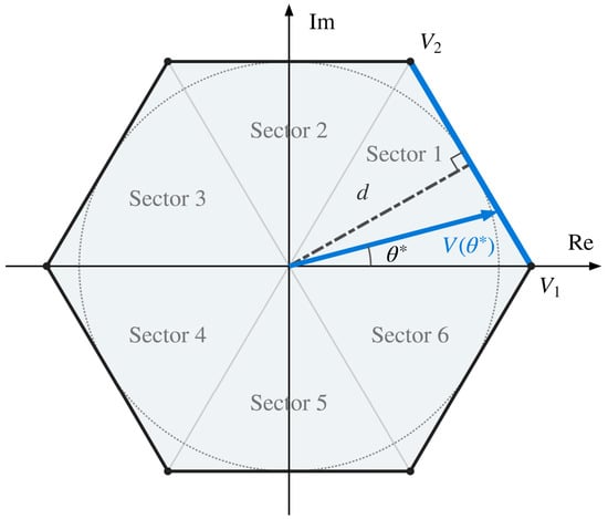
Two angles are used in this paper. The electrical angle $\theta$ increases uniformly with time, and the reference angle ${\theta }^{\mathrm{*}}$ gives the direction of the voltage vector at that electrical angle. The DC-link voltage is normalized to 1 for convenience of calculation. The magnitudes the voltage vector can produce form a hexagon, and with this normalization the distance from its center to a vertex is ${\displaystyle \frac{2}{3}}$. In overmodulation region II, the voltage vector lies on the side of the hexagon, so the direction determines its magnitude. The distance from the center to the hexagon side in a given direction is all the voltage that can be produced there. This distance is the maximum voltage magnitude $V({\theta }^{\mathrm{*}})$ [14].

$$V({\theta }^{\mathrm{*}})={\displaystyle \frac{1}{\sqrt{3}\cos \left(\frac{\pi }{6}-{\theta }^{\mathrm{*}}\right)}}$$

(1)

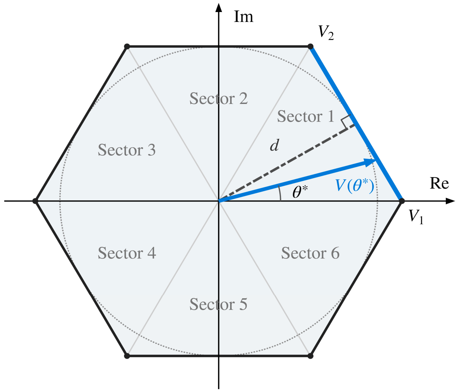
As shown in Figure 1, the hexagon consists of six equilateral triangles, and one equilateral triangle is called a sector. The perpendicular distance $d$ from the center to each side is ${\displaystyle \frac{1}{\sqrt{3}}}$. The angle between this perpendicular and the voltage vector is ${\displaystyle \frac{\pi }{6}}-{\theta }^{\mathrm{*}}$. These two give Equation (1). Owing to the three-phase symmetry and the periodicity, the six sectors are identical to one another, so only one sector has to be treated. Within one sector as well, the maximum voltage magnitude has the same value on both sides of ${\displaystyle \frac{\pi }{6}}$. This is because the cosine in Equation (1) is an even function. Therefore, the range over which the maximum voltage magnitude has to be computed is reduced to $0\le {\theta }^{\mathrm{*}}\le {\displaystyle \frac{\pi }{6}}$.

$$V^{\prime }({\theta }^{\mathrm{*}})=-V({\theta }^{\mathrm{*}})\mathrm{t}\mathrm{a}\mathrm{n} \left({\displaystyle \frac{\pi }{6}}-{\theta }^{\mathrm{*}}\right)$$

(2)

Figure 1. Voltage vector hexagon and the maximum voltage magnitude in the direction of the reference angle. (The blue arrow is the reference voltage vector $V({\theta }^{\mathrm{*}})$, and the blue line is the voltage boundary of Sector 1.

Equation (2) is the derivative of the maximum voltage magnitude with respect to the direction, and it is negative for $0\le {\theta }^{\mathrm{*}}\le {\displaystyle \frac{\pi }{6}}$. The maximum voltage magnitude is the largest at the vertex and decreases monotonically toward the middle of the side. The modulation index is defined as the fundamental component magnitude $c_1$ of the output voltage divided by the six-step fundamental component ${\displaystyle \frac{2}{\pi }}$.

$$m={\displaystyle \frac{c_1}{\frac{2}{\pi }}}$$

(3)

According to Equation (3), overmodulation region I runs from 0.9069 to 0.9514, overmodulation region II from 0.9514 to 1, and 1 is six-step operation [14].

2.2. Placement of the Reference Angle by the Holding Angle and the Step Angles

The reference angle is either fixed at a certain angle or moves along the side. The angle at which the reference angle starts to move along the side is called the holding angle ${\alpha }_h$ [9,10]. The sector is symmetric about ${\displaystyle \frac{\pi }{6}}$, so the reference angle is fixed from $0$ to ${\alpha }_h$ and from ${\displaystyle \frac{\pi }{3}}-{\alpha }_h$ to ${\displaystyle \frac{\pi }{3}}$. From ${\alpha }_h$ to ${\displaystyle \frac{\pi }{3}}-{\alpha }_h$, the reference angle follows the electrical angle. The value at which the reference angle remains is called the step angle ${\alpha }_i$. Here, $i$ is an integer from $1$ to the number of steps $n$. Uniform placement divides ${\alpha }_h$ into $n$ equal parts and assigns one step angle to each.

$$\overrightarrow{V}(\theta )=\left\{\begin{array}{ll}{\displaystyle \frac{2}{3}},& 0\le \theta <{\displaystyle \frac{{\alpha }_h}{n}}\\ ⋮& ⋮\\ V \left({\displaystyle \frac{{\alpha }_h}{n}}(i-1)\right)e^{j{\displaystyle \frac{{\alpha }_h}{n}}(i-1)},& {\displaystyle \frac{{\alpha }_h}{n}}(i-1)\le \theta <{\displaystyle \frac{{\alpha }_h}{n}}\hspace{0.17em}i\\ V\left(\theta \right)\hspace{0.17em}{e}^{j\theta },& {\alpha }_h\le \theta <{\displaystyle \frac{\pi }{3}}-{\alpha }_h\\ V \left({\displaystyle \frac{{\alpha }_h}{n}}(i-1)\right)e^{j\left({\displaystyle \frac{\pi }{3}}-{\displaystyle \frac{{\alpha }_h}{n}}(i-1)\right)},& {\displaystyle \frac{\pi }{3}}-{\displaystyle \frac{{\alpha }_h}{n}}\hspace{0.17em}i\le \theta <{\displaystyle \frac{\pi }{3}}-{\displaystyle \frac{{\alpha }_h}{n}}(i-1)\\ ⋮& ⋮\\ {\displaystyle \frac{2}{3}}\hspace{0.17em}{e}^{j{\displaystyle \frac{\pi }{3}}},& {\displaystyle \frac{\pi }{3}}-{\displaystyle \frac{{\alpha }_h}{n}}\le \theta <{\displaystyle \frac{\pi }{3}}\end{array}\right.i=1,\dots ,n$$

(4)

The fundamental component of Equation (4) is matched to that of the reference. This fixes the holding angle as a function of the modulation index and the number of steps. The step angles follow by dividing that angle into $n$ equal parts. In uniform placement, the number of steps must fall as the voltage rises to maintain voltage linearity. Like uniform placement, the proposed method moves the reference angle in several steps rather than all at once. The electrical angle occupied by one step is also the holding angle divided by $n$. However, the step angles themselves are left as independent variables to be determined.

$${\theta }^{\mathrm{*}}(\theta )=\left\{\begin{array}{ll}{\alpha }_i,& {\displaystyle \frac{{\alpha }_h}{n}}(i-1)\le \theta <{\displaystyle \frac{{\alpha }_h}{n}}i\\ \theta ,& {\alpha }_h\le \theta <{\displaystyle \frac{\pi }{3}}-{\alpha }_h\\ {\displaystyle \frac{\pi }{3}}-{\alpha }_i,& {\displaystyle \frac{\pi }{3}}-{\displaystyle \frac{{\alpha }_h}{n}}i\le \theta <{\displaystyle \frac{\pi }{3}}-{\displaystyle \frac{{\alpha }_h}{n}}(i-1)\end{array}\right. i=1,\dots ,n$$

(5)

$$\overrightarrow{V}\left(\theta \right)=V\left({\theta }^{\mathrm{*}}\left(\theta \right)\right)\hspace{0.17em}{e}^{j{\theta }^{\mathrm{*}}\left(\theta \right)}$$

(6)

Equation (5) indicates where the reference angle is placed at each step. Equation (6) is the voltage vector corresponding to that reference angle.

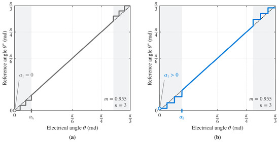
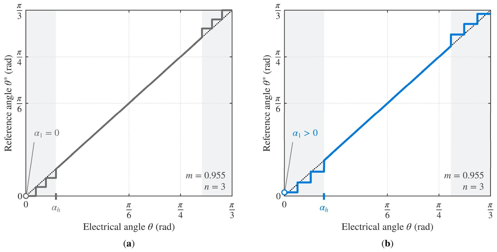
In Figure 2a the first step angle is fixed at the vertex, and in Figure 2b no step angle is located at the vertex. In the proposed method, whether a step angle coincides with the vertex depends on the modulation index. Both panels are drawn at the same modulation index and with the same number of steps, and only the placement is changed. The holding angle differs as a result, and so does the electrical angle occupied by one step. In Figure 2a, the reference angle leaves the vertex only after the first step, and in Figure 2b it never reaches the vertex.

Figure 2. Reference angle according to the electrical angle ($m=0.955$, $n=3$): (a) uniform placement; (b) the proposed method.

3. Derivation and Implementation of the Step Angles and the Holding Angle

3.1. Fundamental Component and THD

The lowest-THD placement satisfying voltage linearity is needed. The fundamental component magnitude and the THD are written as functions of the step angles and the holding angle. The output voltage vector repeats every ${\displaystyle \frac{\pi }{3}}$, so integrating over only one sector and multiplying by ${\displaystyle \frac{3}{\pi }}$ gives the fundamental component. The holding angle divides that integral into three parts. Over the step angles, the imaginary part cancels by symmetry, so only twice the real part remains. Where the reference angle follows the electrical angle, the exponential term disappears and that part is real.

$$\begin{array}{cc}\hfill c_1& ={\displaystyle \frac{3}{\pi }}{\int }_0^{{\displaystyle \frac{\pi }{3}}}\overrightarrow{V}(\theta )\hspace{0.17em}{e}^{-j\theta }\hspace{0.17em}d\theta \hfill \\ \hfill & ={\displaystyle \frac{3}{\pi }}\cdot 2\left[\hspace{0.25em}\mathrm{R}\mathrm{e} \left({\int }_0^{{\alpha }_h}\overrightarrow{V}\left(\theta \right)\hspace{0.17em}{e}^{-j\theta }\hspace{0.17em}d\theta \right)+{\displaystyle \frac{1}{2}}{\int }_{{\alpha }_h}^{{\displaystyle \frac{\pi }{3}}-{\alpha }_h}\overrightarrow{V}(\theta )\hspace{0.17em}{e}^{-j\theta }\hspace{0.17em}d\theta \hspace{0.25em}\right]\hfill \\ \hfill & ={\displaystyle \frac{3}{\pi }}\left[4\sin {\displaystyle \frac{{\alpha }_h}{2n}}{\displaystyle \sum _{i=1}^n}V({\alpha }_i)\hspace{0.17em}\cos \left({\displaystyle \frac{{\alpha }_h}{n}}\left(i-{\displaystyle \frac{1}{2}}\right)-{\alpha }_i\right)+{\displaystyle \frac{2}{\sqrt{3}}}\hspace{0.17em}\mathrm{l}\mathrm{n}\left(\sec \left({\displaystyle \frac{\pi }{6}}-{\alpha }_h\right)+\mathrm{t}\mathrm{a}\mathrm{n}\left({\displaystyle \frac{\pi }{6}}-{\alpha }_h\right)\right)\right]\hfill \\ \hfill & =m\cdot {\displaystyle \frac{2}{\pi }}\hfill \end{array}$$

(7)

Equation (7) is the result of that integration. Step angles and a holding angle satisfying it must be obtained before voltage linearity can be maintained.

Evaluating the THD directly from its definition leads to an infinite series with no closed form. Parseval’s theorem is used [15]. It states that the mean-square value over one period equals the sum of the squared magnitudes of all the components.

$$\begin{array}{cc}\hfill \overline{V^2}& =\hspace{0.33em}{\displaystyle \frac{6}{2\pi }}{\int }_0^{{\displaystyle \frac{\pi }{3}}}V({\theta }^{\mathrm{*}}{)}^2\hspace{0.17em}d\theta \hfill \\ \hfill & =\hspace{0.33em}{\displaystyle \frac{3}{\pi }}\left[\hspace{0.25em}{\displaystyle \frac{2{\alpha }_h}{n}}{\displaystyle \sum _{i=1}^n}V({\alpha }_i{)}^2\hspace{0.25em}+\hspace{0.25em}{\displaystyle \frac{2}{3}}\mathrm{t}\mathrm{a}\mathrm{n} \left({\displaystyle \frac{\pi }{6}}-{\alpha }_h\right)\right]\hfill \\ \hfill & =\hspace{0.33em}\sum _k|c_k{|}^2\hfill \end{array}$$

(8)

This quantity is referred to as the average power of the voltage vector magnitude. Here, $c_1$ is the fundamental component and the remaining $c_k$ are the harmonic components.

$$\begin{array}{cc}\hfill {\mathrm{T}\mathrm{H}\mathrm{D}}^2& ={\displaystyle \frac{\sum _{k\ne 1}|c_k{|}^2}{|c_1{|}^2}}={\displaystyle \frac{\left(\sum _k|c_k{|}^2\right)-|c_1{|}^2}{|c_1{|}^2}}\hfill \\ \hfill & ={\displaystyle \frac{\overline{V^2}-|c_1{|}^2}{|c_1{|}^2}}\hfill \end{array}$$

(9)

Substituting Equation (8) into the definition of the THD removes the infinite series and yields Equation (9). Under voltage linearity, Equation (7) sets the fundamental component magnitude at $m\cdot {\displaystyle \frac{2}{\pi }}$. The denominator and the subtracted value in Equation (9) are then both constants, so reducing the average power is the same as reducing the THD.

3.2. Placement Condition for the Step Angles

Moving a step angle to lower the THD without losing voltage linearity changes the fundamental component. The holding angle is then adjusted so that the fundamental component matches the target modulation index again.

$${\displaystyle \frac{\partial \hspace{0.17em}\overline{V^2}}{\partial {\alpha }_i}}={\displaystyle \frac{12\hspace{0.17em}{\alpha }_h}{n\pi }}\hspace{0.17em}V({\alpha }_i)\hspace{0.17em}{V}^{\prime }({\alpha }_i)$$

(10)

$${\displaystyle \frac{\partial c_1}{\partial {\alpha }_i}}={\displaystyle \frac{12}{\pi }}\sin {\displaystyle \frac{{\alpha }_h}{2n}}\left[\hspace{0.17em}V({\alpha }_i)\sin \left({\displaystyle \frac{{\alpha }_h}{n}}\left(i-{\displaystyle \frac{1}{2}}\right)-{\alpha }_i\right)+V^{\prime }({\alpha }_i)\cos \left({\displaystyle \frac{{\alpha }_h}{n}}\left(i-{\displaystyle \frac{1}{2}}\right)-{\alpha }_i\right)\right]$$

(11)

$${\displaystyle \frac{\partial \hspace{0.17em}\overline{V^2}}{\partial {\alpha }_h}}={\displaystyle \frac{6}{n\pi }}{\displaystyle \sum _{i=1}^n}V({\alpha }_i{)}^2-{\displaystyle \frac{6}{\pi }}\hspace{0.17em}V({\alpha }_h{)}^2$$

(12)

$$\begin{array}{c}{\displaystyle \frac{\partial c_1}{\partial {\alpha }_h}}={\displaystyle \frac{3}{\pi }}\left[\hspace{0.17em}{\displaystyle \frac{2}{n}}\cos {\displaystyle \frac{{\alpha }_h}{2n}}{\displaystyle \sum _{i=1}^n}V({\alpha }_i)\cos \left({\displaystyle \frac{{\alpha }_h}{n}}\left(i-{\displaystyle \frac{1}{2}}\right)-{\alpha }_i\right)\right.\\ \left.-\hspace{0.17em}4\sin {\displaystyle \frac{{\alpha }_h}{2n}}{\displaystyle \sum _{i=1}^n}{\displaystyle \frac{i-\frac{1}{2}}{n}}\hspace{0.17em}V({\alpha }_i)\sin \left({\displaystyle \frac{{\alpha }_h}{n}}\left(i-{\displaystyle \frac{1}{2}}\right)-{\alpha }_i\right)-2\hspace{0.17em}V({\alpha }_h)\hspace{0.17em}\right]\end{array}$$

(13)

Equations (10)–(13) differentiate the average power and the fundamental component with respect to the $n$ step angles and the one holding angle. All four are expressed in terms of the maximum voltage magnitude and its derivative.

$$d{c}_1={\displaystyle \sum _{i=1}^n}{\displaystyle \frac{\partial c_1}{\partial {\alpha }_i}}\hspace{0.17em}d{\alpha }_i+{\displaystyle \frac{\partial c_1}{\partial {\alpha }_h}}\hspace{0.17em}d{\alpha }_h=0$$

(14)

$$d\overline{V^2}={\displaystyle \sum _{i=1}^n}\left({\displaystyle \frac{\partial \hspace{0.17em}\overline{V^2}}{\partial {\alpha }_i}}-{\displaystyle \frac{\frac{\partial \hspace{0.17em}\overline{V^2}}{\partial {\alpha }_h}}{\frac{\partial c_1}{\partial {\alpha }_h}}}\hspace{0.17em}{\displaystyle \frac{\partial c_1}{\partial {\alpha }_i}}\right)d{\alpha }_i$$

(15)

For voltage linearity, the change in the fundamental component must be 0, so Equation (14) holds. The holding angle is thus not an independent variable but a dependent one set by the step angles. Solving Equation (14) for $d{\alpha }_h$ and substituting it into the change in the average power removes the holding angle change, as in Equation (15). The coefficient of $d{\alpha }_i$ in Equation (15) represents the net change in the average power when a single step-angle is moved. The holding angle is readjusted at the same time to restore voltage linearity. Because the average power and the THD vary together according to Equation (9), this coefficient is referred to as the THD sensitivity. Note that a step angle cannot move outward beyond the vertex.

A step angle not located at the vertex can move to either side. A nonzero THD sensitivity would then let the average power fall further. The THD sensitivity must be 0 at the lowest THD. A step angle at the vertex can only move inward from it. Its THD sensitivity need not be 0. Leaving it there is optimal when a small inward move does not reduce the average power. Multiplying both cases by the denominator ${\displaystyle \frac{\partial c_1}{\partial {\alpha }_h}}$ of Equation (15) gives Equation (16), the necessary condition for the lowest-THD placement of the step angles. This denominator is the change in the fundamental component with the holding angle. It is positive for the placements treated here, so the inequality keeps its direction. Voltage linearity moves a step angle outward, while the THD moves it inward.

$$\begin{array}{c}{\alpha }_i>0\hspace{0.25em}\hspace{0.25em}:\hspace{0.25em}\hspace{0.25em}{\displaystyle \frac{\partial \hspace{0.17em}\overline{V^2}}{\partial {\alpha }_i}}\cdot {\displaystyle \frac{\partial c_1}{\partial {\alpha }_h}}\hspace{0.33em}=\hspace{0.33em}{\displaystyle \frac{\partial c_1}{\partial {\alpha }_i}}\cdot {\displaystyle \frac{\partial \hspace{0.17em}\overline{V^2}}{\partial {\alpha }_h}}\\ {\alpha }_i=0\hspace{0.25em}\hspace{0.25em}:\hspace{0.25em}\hspace{0.25em}{\displaystyle \frac{\partial \hspace{0.17em}\overline{V^2}}{\partial {\alpha }_i}}\cdot {\displaystyle \frac{\partial c_1}{\partial {\alpha }_h}}\hspace{0.33em}\ge \hspace{0.33em}{\displaystyle \frac{\partial c_1}{\partial {\alpha }_i}}\cdot {\displaystyle \frac{\partial \hspace{0.17em}\overline{V^2}}{\partial {\alpha }_h}}\end{array}$$

(16)

3.3. Step Angles Coinciding with the Vertex

Equation (16) gives $n$ conditions for lowering the THD, one per step angle. Equation (7) for voltage linearity adds one more, for a total of $n+1$. The unknowns ${\alpha }_1,\dots ,{\alpha }_n,{\alpha }_h$ are also $n+1$ in number. However, Equation (16) becomes an equality or an inequality depending on whether a step angle coincides with the vertex. The number of step angles coinciding with the vertex is denoted by $n_v$. Rather than being fixed in advance, $n_v$ is swept from $0$ to $n$. With $n_v$ step angles placed at the vertex, the holding angle and the step angles are obtained from Equation (7) and Equation (16). If the chosen $n_v$ is too small, some step angles become negative and therefore lie outside the hexagon. If the chosen $n_v$ is too large, a coincident step angle has a negative THD sensitivity. This indicates a position inward from the vertex where the average power can fall further [16]. The candidates are finite, $n+1$ in number, so all are computed. Any candidate with a step angle outside the hexagon or with a reversed order is discarded. The lowest-THD placement is chosen among the remaining candidates.

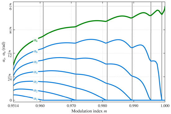
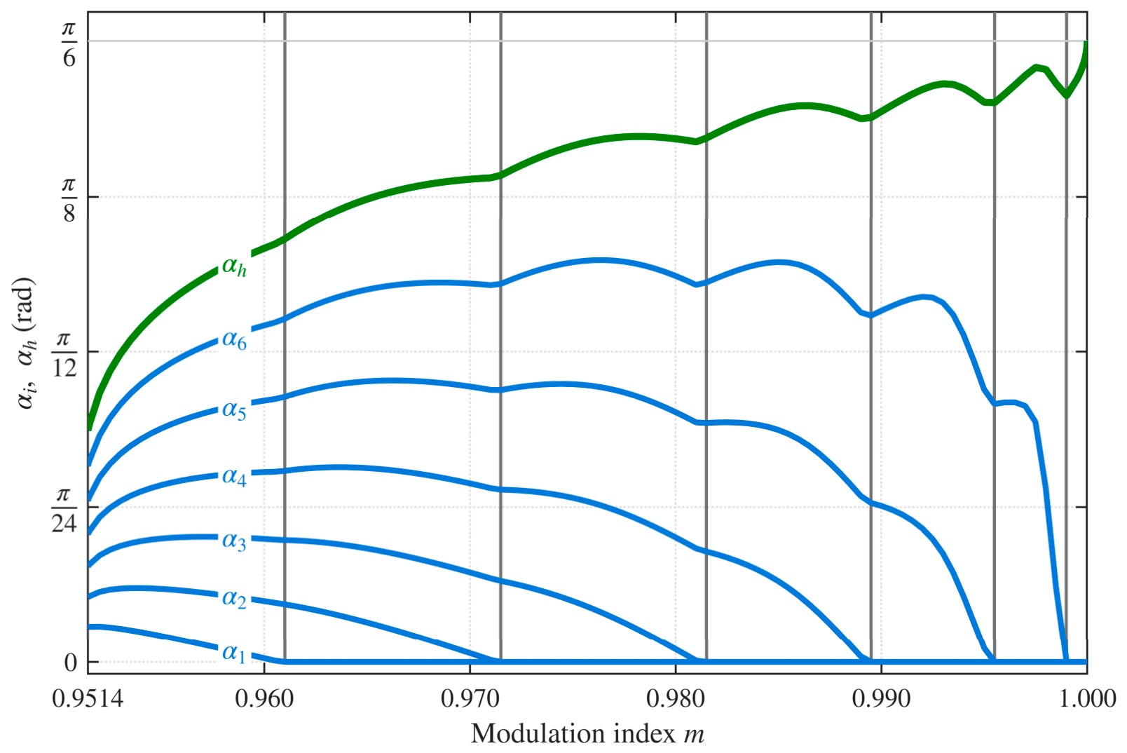
Repeating the calculation at progressively higher modulation indices shows the step angles coinciding with the vertex in turn, as shown in Figure 3. They coincide in order, starting from the one nearest the vertex. A step angle, once located at the vertex, remains there at every higher modulation index. The holding angle follows from voltage linearity once the step angles are fixed. The slope of its curve is thus discontinuous at every modulation index where $n_v$ increases. All steps occupy the same electrical angle. With $n_v$ coincident step angles, the reference angle therefore remains at the vertex for $n_v$ times the width of one step. Coincident step angles are not included in the number of distinct step angles.

Figure 3. Step angles and the holding angle versus the modulation index ($n=6$).

Table 1 divides the modulation index into ranges bounded only by the points where $n_v$ changes. The number of distinct step angles $n_d$ is $n$ when $n_v$ is $0$. It is $(n-n_v)+1$ when $n_v$ is $1$ or more. The number of distinct step angles decreases when $n_v$ is $2$ or more. When $n_v=n$, the reference angle moves directly from the vertex to the holding angle. At $m=1$, the holding angle becomes ${\displaystyle \frac{\pi }{6}}$, half the sector, and all six step angles coincide with the vertex. The result is a six-step waveform whose reference angle stays only at the six vertices. The number of coincident step angles was not prescribed by a rule but followed from solving Equations (7) and (16). The number of distinct step angles falls as part of that solution.

Table 1. Number of coincident step angles and number of distinct step angles in each modulation index range ($n=6$).

Modulation Index $\mathit{m}$	Coincident Step Angles ${\mathit{n}}_{\mathit{v}}$	Distinct Step Angles ${\mathit{n}}_{\mathit{d}}$
$0.9514\le m<0.9610$	0	6
$0.9610\le m<0.9715$	1	6
$0.9715\le m<0.9815$	2	5
$0.9815\le m<0.9895$	3	4
$0.9895\le m<0.9955$	4	3
$0.9955\le m<0.9990$	5	2
$0.9990\le m\le 1$	6	1

3.4. Offline Design and Online Operation

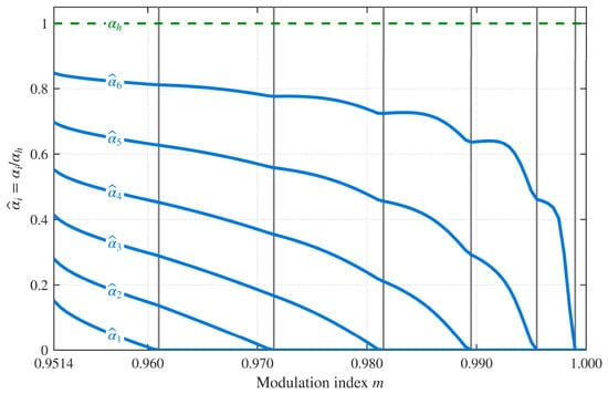
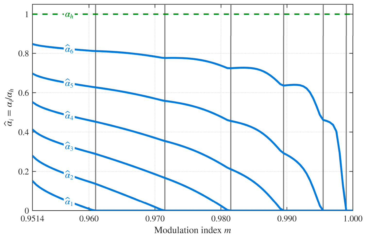
At the design stage, the number of steps is chosen. The $n$ step angles and the one holding angle are then obtained for each modulation index. Each step angle lies between $0$ and the holding angle. The LUT therefore stores the ratio ${\widehat{\alpha }}_i={\alpha }_i/{\alpha }_h$, which lies between $0$ and $1$. Figure 4 shows these normalized step angles. As in Figure 3, the vertical lines mark where a step angle reaches zero and divide the modulation index into ranges.

Figure 4. Normalized step angles versus the modulation index ($n=6$).

In each range, the holding angle and the normalized step angles are approximated by polynomials, and only the coefficients are stored. Once the holding angle has been identified, the step angles follow from those coefficients with arithmetic operations alone.

For each range, the LUT stores the number of coincident step angles $n_v$ and the two end values of the range. The polynomial coefficients of the holding angle and of the normalized step angles are stored as well. If both are approximated to the fifth order, Table 2 lists the number of values to store and the memory for each number of steps.

Table 2. Numbers stored in the LUT and the memory for each number of steps.

Number of Steps $\mathit{n}$	Ranges	Stored Numbers	Bytes (Single)
1	2	24	96
2	3	45	180
3	4	72	288
4	5	105	420
5	6	144	576
6	7	189	756
7	8	240	960

Let $m_0$ be the left end of a range and $m_1$ the right end. The position of the modulation index within it is $\widehat{m}=(m-m_0)/(m_1-m_0)$, which is between $0$ and $1$. In Equation (17), the holding angle and the normalized step angles are approximated by fifth-order polynomials in $\widehat{m}$. The coefficients are specific to each range.

$$\begin{array}{c}{\alpha }_h=a_5{\widehat{m}}^5+a_4{\widehat{m}}^4+a_3{\widehat{m}}^3+a_2{\widehat{m}}^2+a_1\widehat{m}+a_0\\ {\widehat{\alpha }}_i=b_5{\widehat{m}}^5+b_4{\widehat{m}}^4+b_3{\widehat{m}}^3+b_2{\widehat{m}}^2+b_1\widehat{m}+b_0\end{array}$$

(17)

The coefficients in Table 3 are given in radians. Every range uses a fifth-order polynomial, so all seven have the same number of coefficients.

Table 3. Coefficients of the holding-angle polynomial stored in the LUT for each modulation index range ($n=6$).

Range	${\mathit{n}}_{\mathit{v}}$	Modulation Index	${\mathit{a}}_5$	${\mathit{a}}_4$	${\mathit{a}}_3$	${\mathit{a}}_2$	${\mathit{a}}_1$	${\mathit{a}}_0$
1	0	$0.9514$$–0.9610$	$+0.8677$	$-2.4817$	$+2.7545$	$-1.5637$	$+0.5862$	$+0.1957$
2	1	$0.9610$$–0.9715$	$-0.0003$	$-0.0020$	$+0.0292$	$-0.0966$	$+0.1220$	$+0.3568$
3	2	$0.9715$$–0.9815$	$+0.0134$	$-0.0008$	$-0.0319$	$-0.0441$	$+0.0901$	$+0.4108$
4	3	$0.9815$$–0.9895$	$+0.0986$	$-0.1825$	$+0.0631$	$-0.0388$	$+0.0725$	$+0.4421$
5	4	$0.9895$$–0.9955$	$+0.3247$	$-0.7061$	$+0.4314$	$-0.1153$	$+0.0717$	$+0.4593$
6	5	$0.9955$$–0.9990$	$+0.4975$	$-1.2164$	$+0.8689$	$-0.2247$	$+0.0701$	$+0.4718$
7	6	$0.9990$$–1.0000$	$+0.2416$	$-0.5095$	$+0.3901$	$-0.1170$	$+0.0381$	$+0.4773$

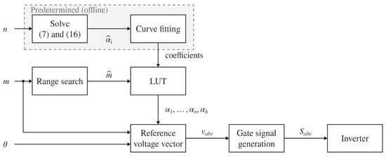
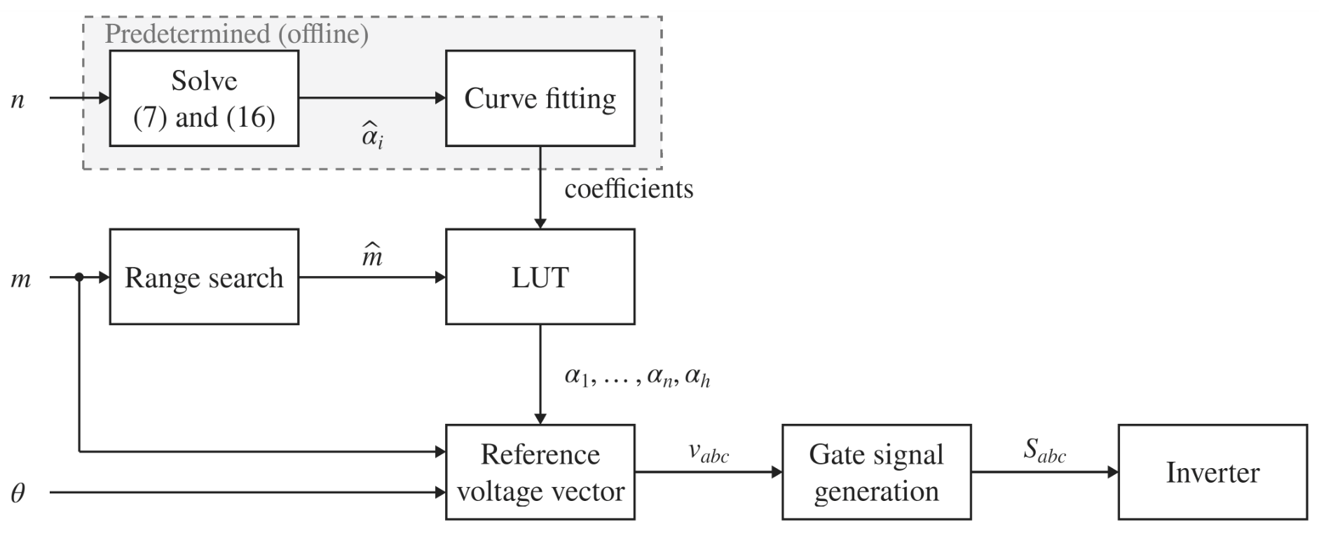
Figure 5 shows the procedure from building the LUT at the design stage to generating the gate signals during operation. At the design stage, the number of steps is chosen, and the normalized step angles follow from Equations (7) and (16). Only their polynomial coefficients are stored in the LUT. During operation, the range in Table 1 containing the reference modulation index is found. The position $\widehat{m}$ within it is computed and substituted into the coefficients of that range. The holding angle comes first, and multiplying it by the normalized step angles gives the step angles, so both angles use arithmetic operations only. Once the two angles and the electrical angle have been determined, the reference voltage vector is fixed. The three-phase reference voltage is obtained from the reference voltage vector. A zero-sequence offset (min-max offset) is then injected to form the pole voltage reference $v_{abc}$. Comparing $v_{abc}$ with the carrier gives the gate signals $S_{abc}$, which are the same as those of SVPWM, without calculating the duty ratios separately.

Figure 5. Flowchart of the control procedure for the offline design and the online operation.

4. Verifications

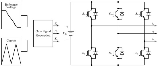
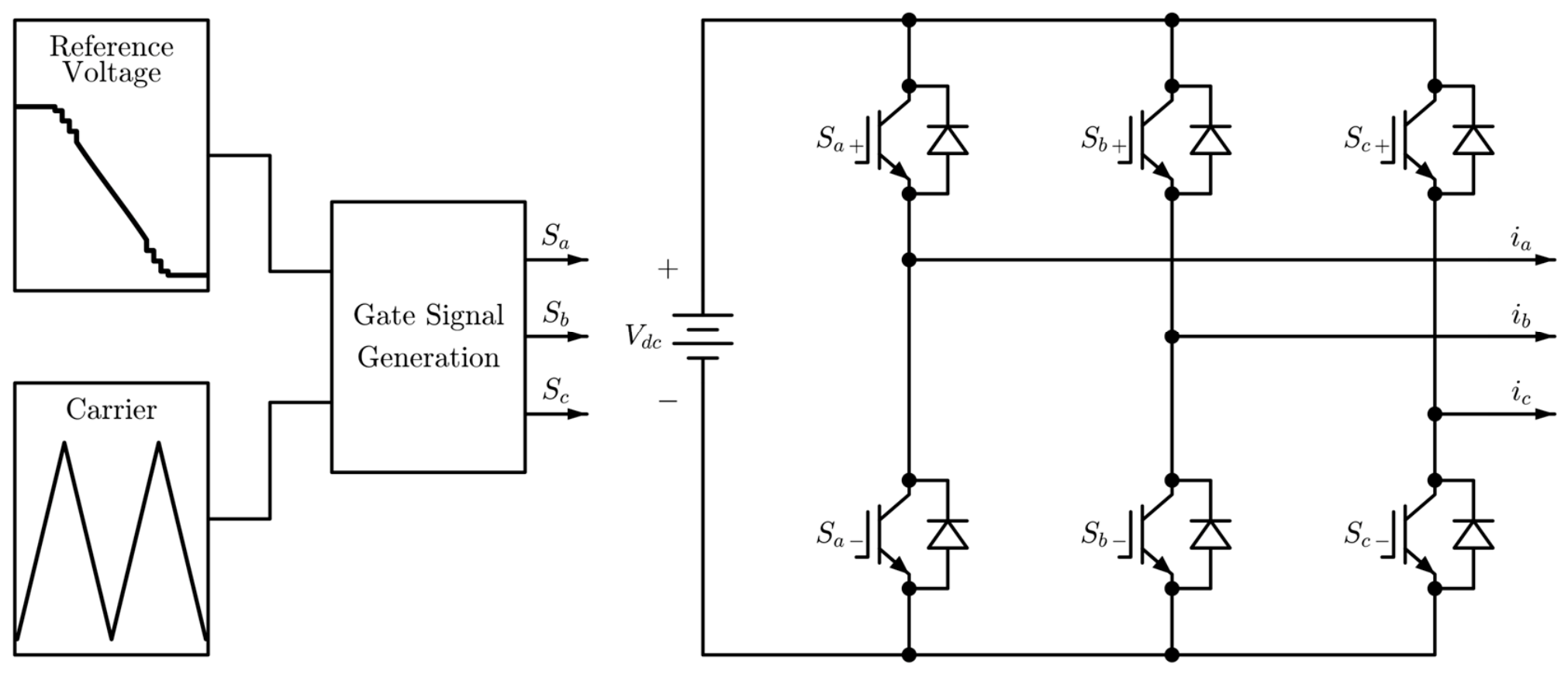
The inverter and motor parameters are listed in Table 4 and the simulation was configured as shown in Figure 6. The circuit is open-loop and the DC-link voltage $V_{dc}$ is a voltage source. The switches are denoted by $S_{a+}$ and $S_{a-}$, where the subscripts give the phase and the upper or lower position. The phase currents flowing out of each leg are $i_a$, $i_b$, and $i_c$.

Table 4. Simulation parameters.

Parameter	Value
Simulation tool	MATLAB/Simulink R2025a
DC-link voltage	590 V
Switching frequency	10 kHz, 50 kHz
Motor	Induction motor, 7.46 kW, 460 V, 60 Hz
Fundamental frequency	100–105 Hz
Rotational speed	2961–3112 rpm

Figure 6. Overall configuration of the simulation.

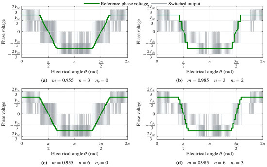
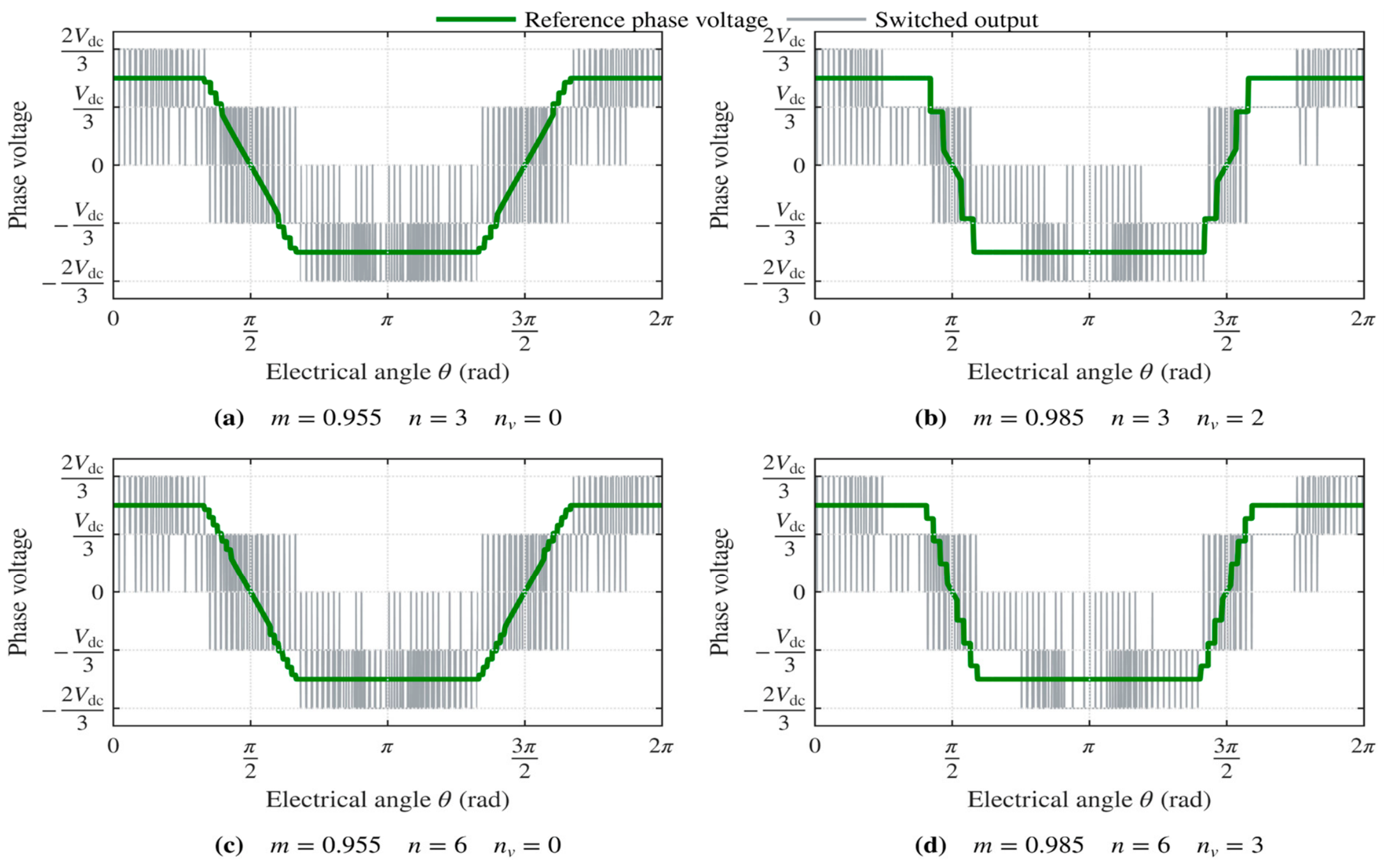
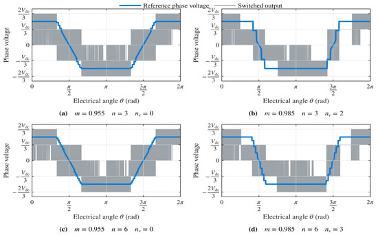
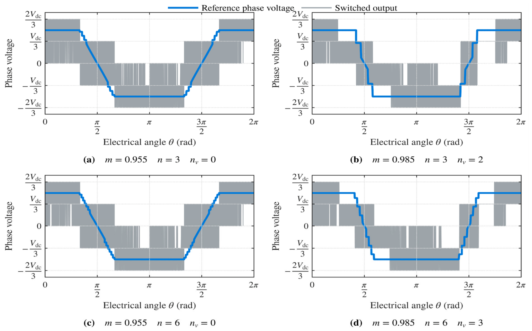
Figure 7 and Figure 8 show the output waveforms at 10 kHz and 50 kHz, respectively. The waveforms are for $n=3$ and $n=6$ at $m=0.955$ and $m=0.985$. The switched phase voltage is in gray. The reference phase voltage is green in Figure 7 and blue in Figure 8. In each figure, comparing (a) with (b) and (c) with (d) shows the number of distinct step angles dropping as the modulation index rises.

Figure 7. Output phase-voltage waveforms (switching frequency 10 kHz): (a) $m=0.955$, $n=3$; (b) $m=0.985$, $n=3$; (c) $m=0.955$, $n=6$; (d) $m=0.985$, $n=6$.

Figure 8. Output phase-voltage waveforms (switching frequency 50 kHz): (a) $m=0.955$, $n=3$; (b) $m=0.985$, $n=3$; (c) $m=0.955$, $n=6$; (d) $m=0.985$, $n=6$.

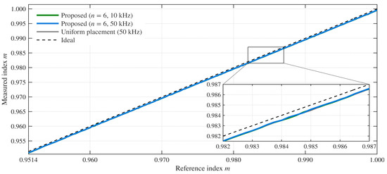
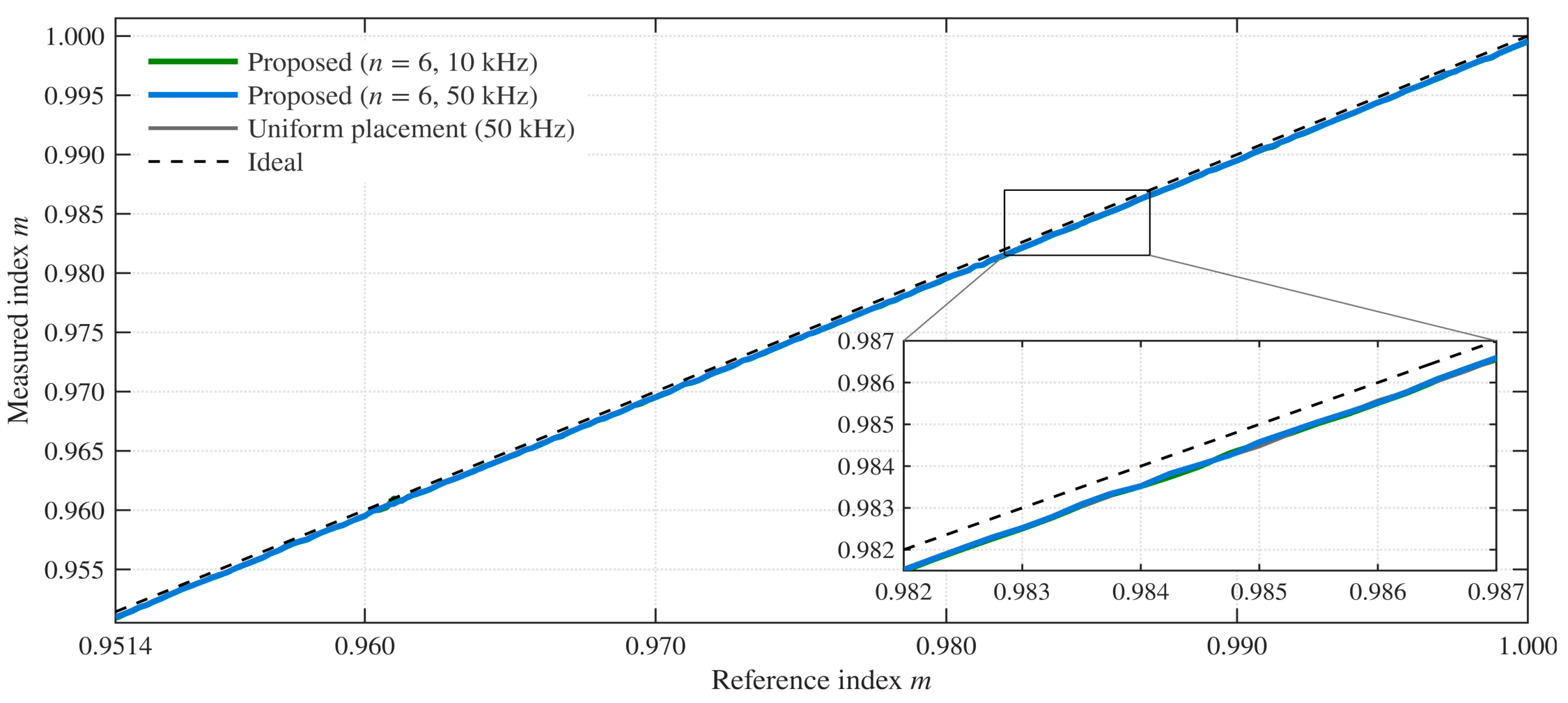
Table 5 lists the reference modulation index and the one measured in the simulation for $n=6$. Figure 9 compares the two throughout overmodulation region II. The difference is smaller at 50 kHz than at 10 kHz, and it is of the order of ${10}^{-4}$ at both switching frequencies. Even for $n$ from 3 to 6, the average difference lies between $4.0\times {10}^{-4}$ and $4.5\times {10}^{-4}$.

Table 5. Reference modulation index and measured modulation index ($n=6$, switching frequencies 10 kHz and 50 kHz).

Reference $\mathit{m}$	Measured (10 kHz)	$\left|\mathrm{Error}\right|$ (${10}^{-4}$)	Measured (50 kHz)	$\left|\mathrm{Error}\right|$ (${10}^{-4}$)
0.9515	0.950965	5.35	0.951032	4.68
0.9550	0.954509	4.91	0.954545	4.55
0.9600	0.959496	5.04	0.959527	4.73
0.9650	0.964528	4.72	0.964559	4.41
0.9700	0.969514	4.86	0.969542	4.58
0.9750	0.974528	4.72	0.974547	4.53
0.9800	0.979552	4.48	0.979585	4.15
0.9850	0.984541	4.59	0.984578	4.22
0.9900	0.989488	5.12	0.989504	4.96
0.9950	0.994528	4.72	0.994548	4.52
1.0000	0.999536	4.64	0.999571	4.29

Figure 9. Measured modulation index versus its reference (the proposed method with $n=6$, uniform placement, and the ideal line; the lower right is an enlarged view).

As shown in Table 5 and Figure 9, the measured modulation index is lower than the reference value over the entire overmodulation region II. This is because the step angles and the holding angle are derived analytically from the ideal stepped waveform. The actual output only approximates that waveform, and the fundamental component is reduced accordingly.

This reduction is a constant offset. It stays below $6\times {10}^{-4}$ at every modulation index, and its average changes by less than $0.3\times {10}^{-4}$ across the ranges of Table 1. It is almost the same at both switching frequencies, and uniform placement gives $4.50\times {10}^{-4}$ at 50 kHz. The size of the offset is therefore set neither by the switching frequency nor by the step placement. In Figure 9, the measured curve is parallel to the ideal line and does not deviate further as the modulation index rises. Voltage linearity is maintained over the whole region apart from this offset.

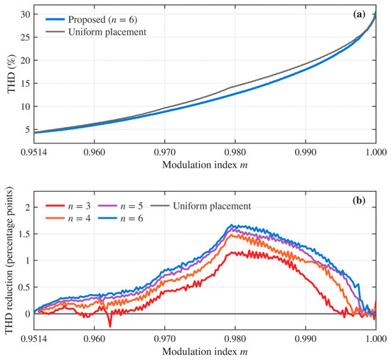
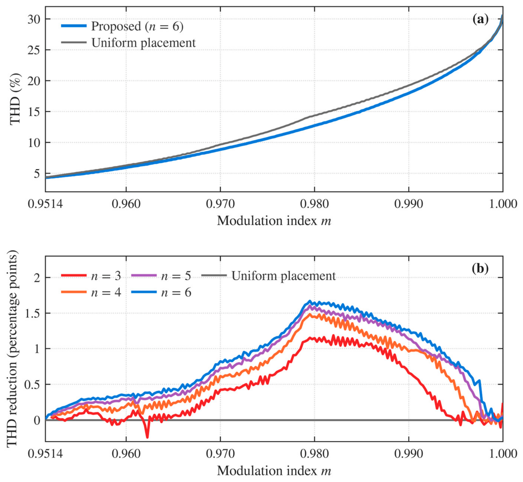
Figure 10a compares the THD of the proposed method with that of uniform placement for $n=6$. Figure 10b shows the THD reduction relative to uniform placement for $n=3$ to $n=6$. The average reduction over the entire overmodulation region II is 0.41, 0.62, 0.75, and 0.82 percentage points for $n=3$, 4, 5, and 6, respectively. A larger number of step angles gives more placements that can lower the THD, so the reduction increases with the number of steps.

Figure 10. THD versus the modulation index (switching frequency 50 kHz): (a) THD of the proposed method with $n=6$ and of uniform placement; (b) reduction in THD with respect to uniform placement (from $n=3$ to $n=6$).

The reduction is the largest in the middle of overmodulation region II. There, the holding angle is wide and few step angles coincide with the vertex. Therefore, the step angles can be placed in the largest number of ways. At the low end, the holding angle is close to zero, so the range for the step angles is narrow. At the high end, most of them coincide with the vertex, so the waveform approaches a six-step waveform. Toward both ends, fewer placements can be chosen, so the reduction becomes smaller.

5. Conclusions

This paper analytically derived the condition for the step placement of the voltage vector in overmodulation region II of a two-level inverter. That placement minimizes the THD while voltage linearity is maintained. Instead of a fixed rule for their positions, the step angles were obtained from the THD sensitivity. The holding angle is a dependent variable determined by voltage linearity. As the modulation index rises, the step angles coincide with the vertex of the hexagon in turn. Coincident step angles merge into a single step. The electrical angle over which the reference angle remains at the vertex was not separately adjusted. Even so, it increases in proportion to the number of coincident step angles. The fall in the number of distinct step angles needs no rule, and the THD-lowering placement produces it automatically. For each modulation index range, the holding angle coefficients and normalized step angle coefficients were stored in the LUT for the chosen number of steps. The LUT is a function of the modulation index alone, so it does not change during operation. The two angles are computed with arithmetic operations.

In the simulations performed with different numbers of steps and switching frequencies, voltage linearity was maintained. The THD was lower than that of uniform placement at most modulation indices. The reduction averaged 0.41 percentage points for $n=3$ and 0.82 percentage points for $n=6$, growing with the number of steps. The step angles can be placed in the largest number of ways in the middle of overmodulation region II, so the reduction was largest there. At the low end, the holding angle is close to zero, and at the high end the waveform approaches a six-step waveform. Fewer placements can be chosen at either end, and the reduction was smaller there. These results confirmed that the THD can be lowered further, with voltage linearity maintained, when no fixed rule sets the step angle positions.

References

- Hava, A.M.; Kerkman, R.J.; Lipo, T.A. Carrier-Based PWM-VSI Overmodulation Strategies: Analysis, Comparison, and Design. IEEE Trans. Power Electron. 1998, 13, 674–689. [Google Scholar] [CrossRef] [Scilit]
- Kerkman, R.J.; Leggate, D.; Seibel, B.J.; Rowan, T.M. Operation of PWM Voltage Source-Inverters in the Overmodulation Region. IEEE Trans. Ind. Electron. 1996, 43, 132–141. [Google Scholar] [CrossRef] [Scilit]
- Hava, A.M.; Sul, S.-K.; Kerkman, R.J.; Lipo, T.A. Dynamic Overmodulation Characteristics of Triangle Intersection PWM Methods. IEEE Trans. Ind. Appl. 1999, 35, 896–907. [Google Scholar] [CrossRef] [Scilit]
- Guo, X.; He, M.; Yang, Y. Over Modulation Strategy of Power Converters: A Review. IEEE Access 2018, 6, 69528–69544. [Google Scholar] [CrossRef] [Scilit]
- Stumpf, P.; Halász, S. Optimization of PWM for the Overmodulation Region of Two-Level Inverters. IEEE Trans. Ind. Appl. 2018, 54, 3393–3404. [Google Scholar] [CrossRef] [Scilit]
- Ren, J.; Liu, L.; Sun, Y.; Li, J.; Chen, H. Research on Flux-Weakening Strategy of Permanent Magnet Synchronous Motor Based on Overmodulation Region II Voltage Harmonic Optimization. In Proceedings of the 2023 IEEE PELS Students and Young Professionals Symposium (SYPS); Institute of Electrical and Electronics Engineers (IEEE): New York, NY, USA, 2023. [Google Scholar] [CrossRef] [Scilit]
- Hwang, C.; Lim, G.C.; Lee, S.; Moon, J.-J.; Park, K.-S.; Ha, J.-I. Synchronous Overmodulation with Less Switchings Including Six-Step Operation. IEEE Trans. Ind. Electron. 2024, 71, 11967–11977. [Google Scholar] [CrossRef] [Scilit]
- Jing, T.; Maklakov, A.; Radionov, A.; Gasiyarov, V.; Liang, Y. Formulations, Solving Algorithms, Existing Problems and Future Challenges of Pre-Programmed PWM Techniques for High-Power AFE Converters: A Comprehensive Review. Energies 2022, 15, 1696. [Google Scholar] [CrossRef] [Scilit]
- Holtz, J.; Lotzkat, W.; Khambadkone, A.M. On Continuous Control of PWM Inverters in the Overmodulation Range Including the Six-Step Mode. IEEE Trans. Power Electron. 1993, 8, 546–553. [Google Scholar] [CrossRef] [Scilit]
- Lee, D.-C.; Lee, G.-M. A Novel Overmodulation Technique for Space-Vector PWM Inverters. IEEE Trans. Power Electron. 1998, 13, 1144–1151. [Google Scholar] [CrossRef] [Scilit]
- Bakhshai, A.R.; Joós, G.; Jain, P.K.; Jin, H. Incorporating the Overmodulation Range in Space Vector Pattern Generators Using a Classification Algorithm. IEEE Trans. Power Electron. 2000, 15, 83–91. [Google Scholar] [CrossRef] [Scilit]
- Großmann, D.; Herold, J.; Zatocil, H.; Griepentrog, G. Analytical Description and Voltage Accuracy Improvement for Natural Overmodulation Methods Applied on a Two-Level Voltage Source Inverter. In Proceedings of the 2026 IEEE Applied Power Electronics Conference and Exposition (APEC); Institute of Electrical and Electronics Engineers (IEEE): New York, NY, USA, 2026; pp. 279–286. [Google Scholar] [CrossRef] [Scilit]
- Lee, D.-M. Advanced Static over-Modulation Scheme Using Offset Voltages Injection for Simple Implementation and Less Harmonics. J. Electr. Eng. Technol. 2015, 10, 138–145. [Google Scholar] [CrossRef] [Scilit]
- Lee, D.-M.; Jung, J.-W.; Kwak, S.-S. Simple Space Vector PWM Scheme for 3-Level NPC Inverters Including the Overmodulation Region. J. Power Electron. 2011, 11, 688–696. [Google Scholar] [CrossRef] [Scilit][Green Version]
- Dordevic, O.; Jones, M.; Levi, E. Analytical Formulas for Phase Voltage RMS Squared and THD in PWM Multiphase Systems. IEEE Trans. Power Electron. 2015, 30, 1645–1656. [Google Scholar] [CrossRef] [Scilit]
- Zhao, L.; Huang, S.; Zheng, J.; Gao, Y. A Harmonic Suppression SVPWM Strategy for the Asymmetric Six-Phase Motor Fed by Two-Level Six-Phase VSI Operating in the Overmodulation Region. Energies 2022, 15, 7589. [Google Scholar] [CrossRef] [Scilit]
Disclaimer/Publisher’s Note: The statements, opinions and data contained in all publications are solely those of the individual author(s) and contributor(s) and not of MDPI and/or the editor(s). MDPI and/or the editor(s) disclaim responsibility for any injury to people or property resulting from any ideas, methods, instructions or products referred to in the content. |
© 2026 by the authors. Licensee MDPI, Basel, Switzerland. This article is an open access article distributed under the terms and conditions of the Creative Commons Attribution (CC BY) license.