


Abstract
Three-dimensional (3D) human pose sequences often exhibit coordinate noise, inconsistent bone lengths, and temporal jitter, which cannot be adequately assessed using positional error alone. We propose an offline kinematic–temporal refinement framework integrating reconstruction fidelity, bone-length consistency, multi-order temporal regularization, bilateral segment-length symmetry, and a soft joint range-of-motion constraint. The framework optimizes 3D joint coordinates without using reference poses during optimization and employs matched-weight ablations and progress-dependent weight scheduling. Experiments cover 371 non-overlapping 64-frame windows from two Human3.6M test subjects, using five realizations of independent Gaussian, temporally correlated, and limb-coherent synthetic perturbations. Under independent Gaussian noise, Full-Fixed refinement reduces MPJPE from 23.96 to 10.34 mm and bone-length error from 16.95 to 3.19 mm. MPJPE also decreases from 23.94 to 10.32 mm under limb-coherent perturbations and from 23.91 to 19.05 mm under temporally correlated perturbations. These results show that temporal correlation makes positional correction more challenging, while kinematic constraints improve skeletal consistency with noise-dependent positional trade-offs. Weight scheduling further adjusts temporal errors with small changes in positional accuracy. Overall, the framework enables interpretable offline refinement with explicitly characterized accuracy–structure–motion trade-offs.
1. Introduction
Three-dimensional (3D) human pose estimation aims to recover the spatial locations and skeletal configuration of human joints from images, video, or keypoint observations. Temporal convolutional networks, Transformers, and graph-based architectures have improved the modeling of joint relationships and motion across frames [1,2,3,4]. Frequency-domain pose modeling [5] and non-causal retentive networks [6] have also been investigated as alternative approaches to exploiting temporal information in 3D human pose estimation. Recent approaches have also integrated motion continuity and limb-invariance priors into sequence encoders [7], or used motion-aware graph fusion to improve prediction from noisy detected keypoints [8]. These advances support applications such as motion capture, human–computer interaction, virtual reality, and quantitative motion analysis.
Accurate joint localization, however, does not by itself ensure stable skeletal geometry and coherent trajectories. Coordinate errors can produce frame-to-frame jitter, variations in estimated bone length, and local joint configurations that conflict with predefined kinematic limits. Such artifacts are relevant when refined trajectories are used to compute skeletal geometry or higher-order motion differences. Post-estimation refinement thus provides a complementary means of regulating geometric and temporal properties after an initial 3D pose sequence has been obtained.
Skeletal and motion priors have been explored through both explicit constraints and learned representations. SkeletonPose incorporates skeletal constraints into 3D pose estimation [9], context-based approaches model inter-joint dependencies [10], trajectory optimization introduces kinematic and dynamic priors [11], and kinematics-aware models capture spatial–temporal relationships [12]. Compositional pose regression has represented human poses through connected bone structures [13], while anatomy- and geometry-constrained estimation has incorporated explicit skeletal relationships [14]. For pose refinement, SmoothNet [15] uses temporal information to reduce jitter in estimated poses, while DeciWatch [16] exploits motion continuity for pose denoising and recovery. Recent studies have further incorporated structural and temporal priors into pose modeling. Liu and Wang [17] integrated smoothness and symmetry constraints into the PoseRL-Net framework, whereas Liu and Tang [18] introduced bone-chain and kinematic hierarchy priors into diffusion-based 3D pose estimation. Memon et al. [19] proposed PosePerfect, combining synthetic localization-error correction with anthropometric refinement, while Jiang et al. [20] developed a hierarchy-aware diffusion framework with spatiotemporal denoising. Recent approaches have addressed occlusion through spatio-temporal relative-depth consistency [21], uncertainty-aware temporal and cross-view cues [22], and hierarchical pose representations [23]. Diffusion-based methods have also been applied to 3D human pose estimation [24] and human motion reconstruction from noisy or incomplete observations [25]. Together, these studies demonstrate the relevance of skeletal structure and temporal information across different modeling strategies and motivate further investigation of their explicit contributions to post-estimation pose refinement.
The constraints involved in refinement act on different, potentially competing properties. Bone-length terms regulate segment geometry, temporal terms act on framewise motion differences, bilateral terms restrict differences in corresponding segment lengths, and joint-range penalties respond to predefined angular violations. Because all these terms ultimately influence the same joint coordinates, improved structural consistency need not coincide with reduced positional or motion error. Their incremental effects may also depend on whether the input errors are temporally independent, persistent across frames, or correlated among joints. Recent robustness benchmarks have also examined the effects of occlusion, motion blur, and noisy observations on video-based 3D human pose lifting [26]. Characterizing these interactions requires matched configurations and evaluation measures that distinguish joint position, skeletal geometry, and temporal behavior.
We therefore investigate an offline kinematic–temporal framework that refines existing 3D joint coordinates through window-level iterative optimization. Its objective integrates reconstruction fidelity, bone-length consistency, first- through third-order temporal regularization, bilateral segment-length symmetry, and a soft range-of-motion (ROM) penalty. Bone-length references are estimated from the initial pose window rather than from evaluation ground truth; the ROM term uses unsigned knee and elbow flexion proxies and acts only when their preset bounds are exceeded. Fixed weights and progress-dependent schedules are examined to characterize how the relative influence of these constraints changes during optimization.
To evaluate the proposed framework, we conduct controlled experiments on Human3.6M pose sequences under independent Gaussian, temporally correlated, and limb-coherent perturbations. Matched-weight ablations are designed to examine the individual and combined contributions of the constraints, while conventional filtering and bone-length projection methods provide comparative baselines. Additional analyses investigate parameter sensitivity, motion characteristics, window-boundary behavior, and computational cost. These evaluations are organized around positional accuracy, skeletal consistency, and temporal continuity.
The contributions of this study are threefold. First, we present an explicit multi-constraint formulation for offline 3D coordinate refinement, combining geometric, temporal, bilateral, and soft joint-range priors within a common optimization procedure. Second, we use matched-weight ablations, complementary synthetic error structures, and development-set sensitivity analyses to identify how constraint contributions and position–structure–motion trade-offs vary with the input-error conditions and optimization weights. Third, we provide a multi-metric evaluation against conventional post-processing baselines, including computational cost and detailed trajectory diagnostics, to characterize the operating behavior and practical scope of the proposed framework.
2. Materials and Methods
2.1. Problem Formulation and Overall Framework
Three-dimensional (3D) human pose refinement is formulated as a multi-constraint optimization problem over the joint coordinates of a pose sequence. For a sequence comprising T frames and J joints, the initial pose observations are represented as:
where X0 denotes the initial 3D pose sequence, T and J represent the numbers of frames and joints, respectively, and t and j are the corresponding frame and joint indices. The vector denotes the initial 3D coordinate of joint j at frame t, where ℝ3 represents the three-dimensional Euclidean coordinate space. In this study, T = 64 and J = 17. The refined pose sequence is defined as:
where X represents the refined 3D pose sequence, and xt,j denotes the optimized coordinate of joint j at frame t.
X = {xt,j ∈ ℝ3|t = 1,…,T,j = 1,…,J}
The refinement objective balances fidelity to the initial pose with skeletal consistency, temporal regularization, bilateral structural relationships, and local joint-motion constraints. These terms are integrated into a unified objective function:
where (X) denotes the total refinement loss evaluated on the optimized pose sequence X. Specifically, rec is the reconstruction-fidelity loss, which penalizes deviations from the initial joint coordinates; bone is the bone-length consistency loss, which regulates segment lengths relative to references estimated from the input window; temp is the temporal regularization loss, which penalizes first-, second-, and third-order temporal differences; sym is the bilateral bone-segment symmetry loss, which penalizes length differences between corresponding left and right segments; and ang is the soft joint range-of-motion loss, which penalizes predefined knee and elbow angle violations. The coefficients wrec, wbone, wtemp, wsym, and wang denote the respective non-negative weights of these five loss terms. Their mathematical definitions and weight configurations are detailed in Section 2.2 and Section 2.3, respectively.
(X) = wrecrec + wbonebone + wtemptemp + wsymsym + wangang
The optimization is initialized from X0, and bone-length references are estimated from the same input window. Reference poses are used to construct the controlled perturbations and evaluate the refinement results, while the optimization objective depends only on the initial pose observations and the defined constraints. Each window is optimized independently, with temporal regularization coupling the joint coordinates across frames within the window. The overall refinement procedure is illustrated in Figure 1.
Figure 1.
Overall framework of the proposed kinematic–temporal multi-constraint 3D human pose refinement method.
2.2. Multi-Constraint Objective Function
The adopted 17-joint skeletal topology and the geometric definitions underlying the bone-length, bilateral symmetry, and joint range-of-motion constraints are illustrated in Figure 2.
Figure 2.
Skeletal topology and joint-angle geometry of the adopted 17-joint human pose model. (a) The 17 joints and 16 skeletal segments, with the pelvis as the root joint. Corresponding bilateral segment pairs are marked by Roman numerals: I, thighs; II, shanks; III, upper arms; and IV, forearms. (b) Geometric definition of the unsigned knee and elbow flexion-proxy angle using adjacent bone vectors. The joint indices follow the mapping in Appendix A.
2.2.1. Reconstruction-Fidelity Term
Reconstruction fidelity maintains consistency between the refined pose and the initial 3D observations while allowing coordinate adjustments under the kinematic and temporal constraints. For a sequence containing T frames and J joints, the reconstruction-fidelity loss is defined as:
where ‖∙‖2 denotes the Euclidean norm. The normalization factor averages the squared coordinate differences over all frames, joints, and spatial dimensions. By penalizing deviations from the initial pose X0, the reconstruction-fidelity term regulates the extent of coordinate adjustment induced by the other constraints. Its relative contribution to the overall objective is controlled by wrec, which balances consistency with the input observations against geometric and temporal regularization.
2.2.2. Bone-Length Consistency Constraint
For a given subject, skeletal segment lengths remain approximately constant over a short pose sequence. However, perturbations in 3D joint coordinates may introduce frame-dependent variations in these lengths. To regulate skeletal geometry, we introduce a bone-length consistency constraint over the set B of skeletal segments [9]. For each segment b in B, connecting joints ib and jb, its length at frame t is calculated as:
where the left-hand side represents the length of segment b at frame t, calculated as the Euclidean distance between its two joint endpoints. The reference length of each segment is estimated from the initial pose window using the temporal median:
where the left-hand side denotes the input-derived reference length of segment b, obtained as the temporal median of its initial observed lengths. The temporal median reduces sensitivity to occasional coordinate perturbations while retaining the skeletal scale represented by the input window. The bone-length consistency loss is then defined as:
where |B| denotes the number of skeletal segments, which is 16 in the adopted topology. Each length deviation is normalized by its input-derived reference length, and the squared relative deviations are averaged over all frames and segments. This formulation encourages temporal consistency in skeletal geometry while complementing the reconstruction-fidelity term. The input-derived bone-length reference is distinct from the ground-truth bone lengths used to evaluate geometric accuracy in Section 2.5.1.
2.2.3. Temporal Regularization Constraint
Human motion exhibits temporal dependencies across consecutive frames. Perturbations in 3D joint coordinates can introduce abrupt variations in pose trajectories, particularly in higher-order temporal differences. To regulate these variations, we introduce a temporal regularization term combining first-, second-, and third-order finite differences. For joint j at frame t, the first-order difference is defined as:
where the first-order difference represents the displacement of joint j between consecutive frames. The second-order difference is defined as:
where the second-order difference describes changes between successive first-order displacements. Accordingly, the third-order difference is expressed as:
where the third-order difference captures variations in second-order differences. The multi-order temporal regularization loss is formulated as:
where n denotes the temporal-difference order, taking values of 1, 2, and 3, and βn denotes its corresponding coefficient. The normalization factor 3J(T − n) accounts for the valid frames, joints, and coordinate components at each difference order. The baseline coefficients are β1 = 1, β2 = 2, and β3 = 0.5 and are retained in the main constraint comparisons. Their influence is further examined through development-set sensitivity analyses.
∆xt,j = xt+1,j − xt,j, t = 1,…,T − 1
∆2xt,j=∆xt+1,j−∆xt,j = xt+2,j − 2xt+1,j + xt,j, t = 1,…,T − 2
∆3xt,j = ∆2xt+1,j − ∆2xt,j, t = 1,…,T − 3
The combined temporal term regulates successive coordinate displacements and higher-order trajectory variations. Together with reconstruction fidelity and skeletal constraints, it provides a means of balancing temporal consistency against positional and geometric adjustments during refinement.
2.2.4. Bilateral Bone-Segment Symmetry Constraint
Corresponding left and right skeletal segments generally exhibit comparable lengths, providing a geometric prior for pose refinement. We introduce a bilateral bone-segment symmetry constraint to regulate the length differences between paired segments. Let denote the set of four bilateral segment pairs: thighs, shanks, upper arms, and forearms. For each pair, bR and bL denote the right and left segment indices, respectively, and their lengths at frame t are calculated according to Equation (5). The bilateral symmetry loss is defined as:
where || denotes the number of bilateral segment pairs, with || = 4 in the adopted skeleton. The loss averages the squared length differences over all frames and bilateral pairs. Since the constraint acts on segment lengths, the left and right limbs can retain different joint configurations, orientations, and motion phases. This term complements the bone-length consistency constraint in Equation (7), which regulates individual segment lengths relative to their input-derived reference values.
2.2.5. Soft Joint Range-of-Motion Constraint
Human joints exhibit characteristic ranges of motion (ROM), which can be incorporated into pose refinement as local kinematic priors [27]. We introduce a piecewise soft ROM constraint for the left and right knees and elbows. Let A denote the set of four constrained joint angles, indexed by a. Each angle is defined by three consecutive joints, with the middle joint serving as the angle vertex. The knee angles are determined by the hip–knee–ankle chains, and the elbow angles by the shoulder–elbow–wrist chains. The adjacent vectors u and v extend from the angle vertex to its two neighboring joints. The unsigned flexion-proxy angle at frame t is defined as:
where θt,a denotes the unsigned flexion-proxy angle of constrained joint a at frame t, expressed in degrees, calculated from the angle between the adjacent bone-segment vectors. The proxy approaches 0∘ when the segments are fully extended and increases with joint flexion.
The allowable flexion-proxy ranges are set to 0–165° for the knees and 0–160° for the elbows. These intervals define fixed kinematic bounds for the constrained joints. These empirically selected bounds provide a consistent kinematic reference for the knee and elbow flexion proxies across the evaluated subjects, informed by conventional descriptions of joint range of motion [27]. The magnitude of the angular violation is calculated as:
where the positive-part operator returns the maximum of its argument and zero, and the lower and upper angular limits define the allowable interval for each joint. The violation magnitude ρ is expressed in radians and equals zero for angles within the prescribed range.
To distinguish different degrees of angular deviation, a continuous piecewise penalty is defined as:
where τ1 and τ2 represent violation thresholds of 5° and 15°, respectively, converted to radians. The penalty increases with violation magnitude and is continuously differentiable at the transition thresholds. The thresholds of 5° and 15° divide angular violations into three regions, allowing the piecewise penalty to regulate deviations of different magnitudes. The overall ROM loss is formulated as:
where the penalty is averaged over all frames and summed across the four constrained joint angles. This soft constraint provides a state-dependent kinematic regularizer that complements the bone-length, temporal, and bilateral symmetry terms in the unified refinement objective.
2.3. Weight Scheduling and Coordinate Optimization
2.3.1. Fixed Weights and Progress-Dependent Weight Scheduling
The constraint terms target different aspects of pose refinement, including positional fidelity, skeletal structure, temporal continuity, and local joint motion, and therefore differ in scale and optimization direction. To regulate their relative contributions during joint optimization, we consider fixed-weight and progress-dependent configurations. Fixed weights remain constant throughout optimization, whereas progress-dependent weights modify selected loss terms as optimization proceeds, changing the relative emphasis on data fidelity and local kinematic restrictions. Let k denote the current iteration index and Niter the total number of iterations. The normalized optimization progress is defined as:
where ξk ∈ [0, 1]; values of 0 and 1 correspond to the beginning and end of the optimization process, respectively. For a scheduled loss category c, its weight is linearly interpolated between the initial and target values:
where is the initial weight of loss category c, is the target weight under the primary schedule (κ = 1), and κ is the schedule-amplitude coefficient. The primary configuration uses κ = 1. When κ changes, the magnitude of the weight variation is scaled proportionally relative to the primary schedule; its effect is examined experimentally. The loss weights used for the matched-weight ablation and the full multi-constraint configurations are listed in Table 1.
Table 1.
Loss-weight configurations used in the multi-constraint optimization.
The coefficients in Table 1 are used as empirical baseline settings for the multi-constraint refinement framework. In the matched-weight ablation, the weights of all active constraints are held constant, allowing their incremental contributions to be examined under common weighting conditions. Sensitivity analyses on the development data further examine the effects of individual loss weights and temporal-order coefficients.
Under the primary linear schedule (κ = 1), the reconstruction-fidelity weight decreases from 0.5 to 0.2, allowing greater coordinate adjustments under the geometric and temporal constraints. Meanwhile, the ROM weight increases from 3.0 to 8.0, strengthening the penalty for joint configurations outside the prescribed angular bounds. The bone-length, temporal, and bilateral symmetry weights remain constant at 8.0, 1.0, and 0.5, respectively.
For the full multi-constraint formulation, the fixed-weight configuration retains the initial coefficients in Table 1, whereas the progress-dependent configuration varies only the reconstruction-fidelity and ROM weights. To examine the effect of time-varying weights, the linear schedule is compared with constant weights equal to their mean values and with an alternative cosine weight schedule.
2.3.2. Coordinate Optimization and Solver
After specifying the constraint terms and their weights, we refine each pose window by directly optimizing its 3D joint coordinates, initialized from the input pose sequence. The geometric and temporal constraints act jointly on these coordinates, with temporal regularization coupling the frames within each window. Different windows are optimized independently.
We use Adam for gradient-based coordinate optimization [28]. The initial learning rate is set to 0.003 and reduced to 0.00015 through cosine annealing [29]. To control the influence of large gradients, gradient-norm clipping with a threshold of 1.5 is applied separately to each pose window before the Adam update. The learning-rate schedule spans the prescribed number of iterations for each optimization run.
The main constraint comparisons use a fixed budget of 500 optimization iterations per window. At each iteration, the weighted objective is evaluated from the current joint coordinates, and its gradient is used to update the coordinates through Adam. For progress-dependent configurations, the selected loss weights vary according to Section 2.3.1, while the cosine learning-rate schedule controls the optimizer’s learning rate. The coordinates obtained after the prescribed iterations constitute the refined pose sequence.
2.4. Dataset and Experimental Design
2.4.1. Dataset and Pose-Sequence Preprocessing
Experiments were conducted using available 3D joint-coordinate sequences from the Human3.6M dataset [30]. Seven subjects were represented in this study. Data from S1, S5, S6, S7, and S8 were used for development analyses, including the selection of conventional post-processing baseline configurations and sensitivity analyses of the constraint parameters. The main evaluation was conducted on S9 and S11. Each experimental input consisted of 3D joint coordinates. The coordinates were converted from millimeters to meters before optimization, while the evaluation errors were expressed in millimeters and the corresponding frame-based difference units.
The final evaluation comprised eight 3D pose sequences: Discussion, Eating, Smoking, and Walking for S9, and Discussion, Eating, Smoking, and Waiting for S11. A fixed 32-to-17 joint mapping was applied consistently to the constraint calculations, coordinate optimization, and evaluation metrics. The joint names and original indices are provided in Table A1 of Appendix A. Each sequence was divided chronologically into non-overlapping 64-frame windows, with incomplete trailing segments excluded. Discussion, Eating, and Smoking were evaluated for both subjects, whereas Walking was represented only for S9 and Waiting only for S11. Consequently, comparisons between the latter two actions also reflect differences between subjects. Table 2 summarizes the frame counts and resulting windows for each sequence.
Table 2.
Window partitioning of the Human3.6M evaluation sequences.
The eight sequences yielded 371 complete windows, comprising 23,744 frames from the original 24,064 frames.
2.4.2. Controlled Coordinate Perturbation
To examine how coordinate-error structure affects pose refinement, we considered three types of synthetic perturbations: independent Gaussian noise, temporally correlated noise, and limb-coherent noise. Let denote the reference 3D coordinate of joint j at frame t. Under independent Gaussian perturbations, the input pose is defined as:
where εt,j denotes the three-dimensional perturbation vector, I3 is the identity matrix, and σ = 0.015 m(15 mm) is the standard deviation of each coordinate component. Under this condition, perturbations are sampled independently across frames, joints, and coordinate components.
Temporally correlated perturbations were generated using a stationary first-order autoregressive process (AR(1)) with correlation coefficient ρ = 0.85. For each joint j and coordinate component c, let z denote independent standard normal innovations. The noise process is defined by:
Stationary initialization and innovation scaling retain a theoretical marginal coordinate standard deviation of 15 mm while introducing temporal correlation. Each 64-frame window is initialized independently, with separate random streams for different joints and coordinate components.
Limb-coherent perturbations combine independent joint-specific Gaussian noise with a displacement shared among the joints of each skeletal group. For coordinate component c, the perturbation is defined as:
εt,j,c = ηt,j,c + bt,g(j),c
Here, g(j) identifies one of five non-overlapping skeletal groups: trunk, right leg, left leg, left arm, and right arm. The independent joint-specific component and the group-shared component have standard deviations of 10 mm and √125 mm (approximately 11.18 mm), respectively. These independent components yield a marginal coordinate standard deviation of 15 mm. Each group-shared displacement is resampled at every frame and shared by all joints in the corresponding group.
For each perturbation condition, five random realizations (seeds 0–4) were generated for each of the 371 pose windows, yielding 1855 perturbed inputs per condition. All methods processed the same perturbed input for a given window, condition, and seed. Reference sequences were used to generate the synthetic inputs and evaluate the results; refinement was performed using the perturbed coordinates.
2.4.3. Experimental Settings
The matched-weight ablation compared six constraint combinations on identical 64-frame inputs under independent Gaussian perturbations. The optimizer, cosine learning-rate schedule, 500-iteration budget, and weights of the active loss terms were held constant; only the set of enabled constraints differed across configurations (Table 3).
Table 3.
Matched-weight switch-based ablation configurations.
Reconstruction fidelity was included in all six configurations. A contained no additional constraint; B and C added temporal regularization and bone-length consistency, respectively; D combined both terms; E additionally included bilateral bone-segment symmetry; and F activated the full objective, including ROM. Each enabled term used its fixed coefficient in Table 1. At 500 iterations, F was equivalent to the Full-Fixed configuration.
A separate iteration-budget analysis considered the Temporal, Bone+Temporal, and full multi-constraint formulations. Temporal combined a reconstruction weight scheduled from 0.3 to 0.1 with a temporal weight of 5. Bone+Temporal used constant reconstruction, bone-length, and temporal weights of 1, 8, and 1, respectively. The full formulation was evaluated with the fixed weights in Table 1 and with progress-dependent weights, including scheduling amplitudes κ = 0.8, 1.0, and 1.2. The effect of iteration count was examined through separate 100-, 200-, and 500-iteration runs, with the learning-rate and applicable loss-weight schedules spanning the duration of each run.
The response of the soft ROM constraint was examined separately using controlled directional perturbations. The first, middle, and last 64-frame windows of each of the eight evaluation sequences yielded 24 source windows. For each window, the distal joint of each knee and elbow was rotated by 5°, 10°, 20°, or 30°, giving 384 perturbed inputs. When the original geometry was near the 179.9° angular boundary, an equal-magnitude rotation in the opposite direction was applied. Affected-joint angular error, MPJPE, and ROM violations were evaluated after 100 Adam iterations using only reconstruction fidelity and the ROM penalty. In this isolated experiment, the reconstruction weight decreased from 0.3 to 0.1, and the ROM weight increased from 5 to 10; all other constraint weights were zero.
Seven conventional post-processing configurations were evaluated: Savitzky–Golay (SG), Butterworth, One-Euro, and Kalman filtering; bone-length projection; and SG or Butterworth filtering followed by projection. The SG filter used a 21-frame window and a second-order polynomial, with interpolation at window boundaries. The second-order Butterworth filter used a normalized cutoff frequency of 0.10 relative to the Nyquist frequency and forward–backward filtering with odd padding (padlen = 9). The One-Euro filter used a minimum cutoff of 0.05 frame−1, a β coefficient of 5 m−1, and a derivative cutoff of 0.10 frame−1. The Kalman filter used ρ = 0.01, an observation variance of 0.000225 m2, and an initial velocity variance ratio of 100. Both recursive filters used a discrete time increment of one frame and were initialized independently for each window. Bone-length projection used the temporal median segment lengths estimated from the original perturbed window, with a minimum-length threshold of 10−12 m. For combined methods, filtering preceded bone-length projection.
The baseline parameters were selected from 47 candidates using 300 development inputs from S1, S5, S6, S7, and S8, and were subsequently fixed for evaluation. The seven conventional configurations were compared with the unrefined input, Matched B, Full-Fixed, and Full-Scheduled on the same 1855 independently perturbed S9/S11 inputs. Under temporally correlated and limb-coherent perturbations, the conventional comparisons included SG, Butterworth, and their corresponding bone-projection combinations. No subject-specific parameter adjustments were applied.
Parameter sensitivity was examined separately using 26 configurations on a development panel of 60 windows, comprising three windows from each of four sequences for each of the five development subjects, with five perturbation seeds per window (300 inputs). The analysis varied individual constraint weights, coefficients of the three temporal-difference orders, and weight schedules. In addition to the primary linear schedule, it included a mean-matched fixed configuration (reconstruction weight 0.35 and ROM weight 5.5) and an alternative cosine weight schedule. The main matched-weight configurations remained unchanged.
To investigate whether successive coordinate changes could inform a stopping decision, we used the first 64-frame window of Discussion, Eating, Smoking, and Walking for each of S1, S5, S6, S7, and S8, with seed 0, yielding 20 inputs. Full-Fixed and the primary linear schedule were each evaluated for 500 iterations on these inputs, producing 40 optimization trajectories. The root-mean-square (RMS) coordinate change between successive updates was defined as:
where X(k) denotes the T × J × 3 coordinate array after the k-th update, and ‖·‖F denotes the Frobenius norm over all coordinate components. The factor 1000 converts meters to millimeters. For each threshold τ ∈ {0.01, 0.03, 0.10} mm, the first candidate stopping point was identified after 20 consecutive updates satisfying uk < τ, with the first 100 updates excluded from the count. Candidate stopping iterations were determined from these coordinate changes, and their MPJPE, bone-length error, and jerk error were then compared with those obtained after 500 iterations.
The proposed framework and conventional post-processing methods were implemented in Python (version 3.9.8), using PyTorch (version 2.8.0), NumPy (version 1.24.3), and SciPy (version 1.12.0). Experimental figures were generated using Matplotlib (version 3.8.2). To characterize computational cost, per-window runtimes were measured on an Intel Core i9-12900K CPU (Intel Corporation, Santa Clara, CA, USA) using float64 precision, a batch size of one, and a single computational thread and worker. Three warm-up runs were performed for each method using development-set inputs before timing. Each method was then evaluated on 24 fixed 64-frame windows, with 20 timing repetitions per window. The median of the window-level medians was reported.
To examine motion behavior beyond aggregate errors, we evaluated joint- and action-specific accuracy and reference-free motion magnitudes. Reference-relative temporal-difference errors across adjacent window boundaries were also analyzed to characterize continuity between independently refined segments.
2.5. Evaluation Metrics and Statistical Analysis
2.5.1. Evaluation Metrics
Pose refinement is evaluated in terms of positional accuracy, skeletal consistency, and motion continuity. The primary metrics include mean per-joint position error (MPJPE), bone-length error, and reference-relative velocity, acceleration, and jerk errors. Joint-range compliance is additionally assessed using the angle violation rate (AVR). Let xt,j and denote the refined and reference coordinates of joint j at frame t, respectively. MPJPE is defined as:
MPJPE characterizes absolute positional accuracy across the 17-joint skeleton, including the pelvis root. To assess relative joint configuration independently of global translation, we additionally report root-aligned MPJPE, obtained by centering the refined and reference poses separately at their respective pelvis coordinates. Both measures are expressed in millimeters.
To evaluate skeletal geometric consistency, we calculate the mean absolute difference between refined and reference bone lengths. Let denote the reference length of bone segment b at frame t. The bone-length error is defined as:
To assess motion fidelity, we compute first-, second-, and third-order temporal-difference errors relative to the reference sequence. For difference order n ∈ {1, 2, 3}, the error is defined as:
These three quantities correspond to reference-relative velocity, acceleration, and jerk errors, respectively, following the finite-difference definitions in Section 2.2.3. They are evaluated within each 64-frame window and expressed in mm/frame, mm/frame2, and mm/frame3.
To characterize motion amplitude beyond reference-relative errors, we also examine the magnitudes of first-, second-, and third-order temporal differences, temporal and root-relative RMS amplitudes, joint path length, and temporal bone-length variability. These measurements provide complementary descriptions of trajectory changes and skeletal variation following refinement.
Continuity between independently refined windows is evaluated using reference-relative temporal differences spanning adjacent window boundaries. At each boundary, first-, second-, and third-order differences contribute one, two, and three boundary-spanning positions, respectively. The corresponding errors are examined alongside the within-window measures.
The angle violation rate (AVR) measures the proportion of constrained joint-angle states outside their prescribed ROM intervals. Let 𝕀(⋅) denote the indicator function, equal to 1 when the condition is satisfied and 0 otherwise. AVR is defined as:
AVR characterizes out-of-range states across the left and right knees and elbows. For the controlled directional-perturbation experiment, we additionally evaluate the affected-joint angular mean absolute error. For each perturbed input, the error is computed over the 64 frames between the refined unsigned flexion-proxy angle of the targeted joint a* and its unperturbed reference angle. This metric is reported in degrees.
2.5.2. Statistical Analysis and Multi-Objective Comparison
Statistical comparisons were based on matched pose windows and perturbation realizations. For each window, the evaluation metrics were first averaged across five noise realizations. The resulting window-level values were then averaged within each sequence, and the eight sequence-level estimates were weighted equally to obtain the overall results. Subject-specific and window-weighted summaries were also examined to characterize differences across the evaluation data.
For the matched-weight ablation, six paired contrasts were considered: B − A, C − A, D − B, D − C, E − D, and F − E. Each contrast represents the change in an evaluation metric associated with activating an additional constraint under common weights. The Bone × Temporal interaction contrast, D − B − C + A, was further used to examine the departure of the combined constraint effect from the sum of its individual effects. Effect sizes were expressed as mean paired differences, with negative values indicating error reductions for the six direct contrasts.
For the independent Gaussian matched-weight comparisons, uncertainty intervals were estimated using a non-circular moving-block bootstrap to account for temporal dependence among windows within each sequence. The primary analysis used blocks of four consecutive windows and 10,000 bootstrap replicates. Paired configurations were resampled using the same window indices, and the resulting differences were aggregated with equal weight across the eight sequences. The 2.5th and 97.5th percentiles defined the conditional 95% intervals. Block lengths of two and eight windows were additionally examined to assess sensitivity to the temporal dependence assumption. These intervals quantify conditional uncertainty under temporal resampling of the eight evaluated sequences from S9 and S11.
Because ROM violations occurred infrequently, AVR was summarized descriptively through violation rates and activation frequencies. The positional, skeletal, and temporal errors were examined using their paired effect sizes and corresponding uncertainty intervals.
To characterize multi-objective relationships, Pareto non-dominance was assessed among the evaluated configurations using window-weighted mean metric values at full numerical precision. A configuration was considered non-dominated when no other evaluated configuration achieved equal or lower errors on all selected objectives and a strictly lower error on at least one. The analysis considered three two-objective spaces—MPJPE versus bone-length error, acceleration error, and jerk error—and a three-objective space comprising MPJPE, bone-length error, and jerk error. Following non-dominance-based approaches to multi-objective learning [31,32], these comparisons characterize performance trade-offs among the evaluated refinement configurations.
3. Results
3.1. Overall Results of the Matched-Weight Ablation
Table 4 presents the sequence-equal results of the six matched-weight configurations under independent Gaussian perturbations after 500 optimization iterations.
Table 4.
Sequence-equal evaluation results for the matched-weight ablation configurations.
Configuration A, containing only reconstruction fidelity, yields an MPJPE of 23.962 mm and a bone-length error of 16.954 mm. Adding temporal regularization in configuration B reduces MPJPE to 9.393 mm and jerk error from 107.137 to 2.255 mm/frame3, while bone-length error decreases to 6.448 mm. In contrast, introducing bone-length consistency alone in configuration C reduces bone-length error to 3.232 mm, with MPJPE remaining at 20.900 mm.
Combining temporal regularization and bone-length consistency in configuration D yields a bone-length error of 3.230 mm and an MPJPE of 10.338 mm. Relative to B, this combination improves skeletal geometry while increasing positional and reference-relative temporal errors. The addition of bilateral bone-segment symmetry in configuration E further reduces bone-length error to 3.191 mm, with comparatively small changes in the other metrics. Configuration F, which additionally incorporates the soft ROM constraint, produces nearly identical results at the reported precision.
AVR is 0.000279% for configuration A and zero for configurations B–F. Among the six configurations, B achieves the lowest MPJPE and reference-relative temporal errors, whereas E and F provide the lowest bone-length error. These results reveal distinct trade-offs between positional accuracy, skeletal consistency, and motion fidelity. The corresponding paired effects and uncertainty intervals are examined in Section 3.2.
3.2. Paired Constraint Effects and Conditional Uncertainty Intervals
The paired effects of the individual constraints and the Bone × Temporal interaction are summarized in Table 5. Under the matched-weight conditions, adding temporal regularization to reconstruction fidelity (B − A) reduces MPJPE by 14.568 mm and jerk error by 104.881 mm/frame3, together with a 10.506 mm reduction in bone-length error. In contrast, introducing bone-length consistency alone (C − A) produces a larger reduction in bone-length error of 13.722 mm, but a smaller MPJPE reduction of 3.062 mm.
Table 5.
Sequence-equal paired effects and conditional 95% intervals for the matched-weight ablation.
When bone-length consistency is added to temporal regularization (D − B), bone-length error decreases by 3.217 mm, whereas MPJPE and jerk error increase by 0.944 mm and 0.488 mm/frame3, respectively. Conversely, adding temporal regularization to the bone-length configuration (D − C) reduces MPJPE by 10.562 mm and jerk error by 90.138 mm/frame3, with only a small change in bone-length error. These contrasting effects indicate that the contribution of each constraint depends on the accompanying regularization terms.
The incremental effects of bilateral symmetry and ROM are considerably smaller. Adding the bilateral bone-segment symmetry constraint (E − D) reduces bone-length error by approximately 0.040 mm, with minor changes in positional and temporal errors. The subsequent addition of the soft ROM constraint (F − E) produces changes close to zero across the three metrics, consistent with its limited activation under the evaluated Gaussian perturbations.
The Bone × Temporal interaction contrast (D − B − C + A) is positive for MPJPE, bone-length error, and jerk error, with mean differences of 4.006 mm, 10.505 mm, and 14.743 mm/frame3, respectively. These results indicate a non-additive relationship between the two constraints when applied within the unified optimization framework. Configuration D also achieves substantial reductions in positional, skeletal, and temporal errors relative to reconstruction fidelity alone (A), highlighting the complementary contributions of temporal regularization and bone-length consistency to multi-constraint pose refinement.
3.3. Iteration Budget, Weight Scheduling, and Computation Time
Beyond the matched-weight ablation, we examine the influence of iteration budget and weight scheduling on refinement performance and computation time. The Temporal and Bone+Temporal formulations use the weighting configurations described in Section 2.4.3, whereas the full multi-constraint formulation is evaluated with fixed (Full-Fixed) and progress-dependent (Full-Scheduled) weights.
3.3.1. Refinement Results at Different Iteration Counts
Figure 3 illustrates the effects of iteration budget on MPJPE and bone-length error for the Temporal, Bone+Temporal, Full-Fixed, and Full-Scheduled (κ = 1.0) configurations. The 100-, 200-, and 500-iteration settings were evaluated through separate optimization runs, following the corresponding learning-rate and loss-weight schedules. The results are averaged across the 371 evaluation windows with equal window weights.
Figure 3.
MPJPE (a) and bone-length error (b) under different optimization iteration budgets.
The Temporal configuration exhibits a non-monotonic change in positional accuracy. MPJPE decreases from 10.352 mm at 100 iterations to 9.465 mm at 200 iterations, before increasing to 10.317 mm at 500 iterations. In contrast, its bone-length error decreases from 7.125 to 4.954 mm over the evaluated budgets, indicating different responses of positional and skeletal errors to the number of optimization iterations.
For the Bone+Temporal, Full-Fixed, and Full-Scheduled configurations, MPJPE decreases progressively as the iteration budget increases. Between 100 and 500 iterations, MPJPE decreases from 14.425 to 10.230 mm for Bone+Temporal, from 14.710 to 10.319 mm for Full-Fixed, and from 14.790 to 10.407 mm for Full-Scheduled. Their bone-length errors remain close to 3.2 mm across the evaluated budgets. These results indicate that the influence of iteration budget depends on the constraint combination, with positional accuracy exhibiting greater variation than skeletal geometric consistency when bone-length regularization is included.
3.3.2. Metric Changes Under Progress-Dependent Weight Scheduling
The influence of scheduling amplitude was examined by comparing Full-Scheduled with Full-Fixed at the same iteration budget. Figure 4 illustrates the corresponding changes in MPJPE and jerk error for κ = 0.8, 1.0, and 1.2. Across all three iteration budgets, progress-dependent scheduling produces lower acceleration and jerk errors, accompanied by small increases in MPJPE and bone-length error.
Figure 4.
MPJPE–jerk-error changes under progress-dependent weight scheduling relative to the fixed-weight configuration at different iteration counts. The gray dashed lines indicate zero change in the corresponding metrics.
At 500 iterations, increasing κ from 0.8 to 1.2 raises the MPJPE difference relative to Full-Fixed from 0.061 to 0.122 mm, while the reduction in jerk error increases from 0.364 to 0.519 mm/frame3. The corresponding acceleration-error reductions range from 0.240 to 0.345 mm/frame2. These changes demonstrate how the scheduling amplitude shifts the balance between positional accuracy and temporal motion errors.
Alternative weighting strategies were further compared on the five-subject development data. Among the four weighting strategies, Full-Fixed yields the lowest MPJPE (10.396 mm), whereas the cosine schedule achieves the lowest jerk error (2.232 mm/frame3). The primary linear schedule produces an MPJPE of 10.471 mm and a jerk error of 2.260 mm/frame3, compared with 10.553 mm and 2.431 mm/frame3 under constant mean-matched weights. Bone-length errors remain approximately 3.25 mm across the four configurations. These results indicate that the temporal distribution of loss weights influences refinement performance beyond their average values, with different schedules yielding distinct positional and temporal error trade-offs.
3.3.3. Computation Time
Figure 5 compares the per-window computation times of seven conventional post-processing methods and three iterative refinement configurations under identical single-threaded CPU conditions.
Figure 5.
Median computation time per 64-frame window for conventional post-processing methods and iterative pose-refinement configurations. Blue circles represent conventional post-processing methods, while brown squares represent iterative refinement configurations. The horizontal axis uses a logarithmic scale.
The conventional methods require 0.245–1.119 ms per window, compared with 1358.725 ms for Matched B and 1748.053 and 1747.669 ms for Full-Fixed and Full-Scheduled, respectively. The substantially greater computational cost of the refinement configurations reflects the iterative nature of coordinate optimization. Matched B requires less computation than the full multi-constraint formulations, while Full-Fixed and Full-Scheduled exhibit comparable processing times.
3.4. ROM Constraint Response and Multi-Objective Performance
3.4.1. Response of the ROM Constraint
Under independent Gaussian perturbations, the soft ROM constraint responds selectively to joint configurations that exceed the prescribed angular bounds. In the matched-weight ablation, the sequence-equal AVR is 0.000279% for configuration A and zero for configurations B–F. Among the 1855 matched inputs, five trajectories exhibit nonzero weighted ROM gradients and corresponding coordinate differences between configurations E and F. The near-identical aggregate errors of E and F (Table 5) are consistent with the localized action of the ROM penalty under these conditions.
The response to induced violations was further examined through controlled directional perturbations. Among 384 perturbed inputs, three cases produced new ROM violations, all involving the right elbow in two source windows. The isolated reconstruction-fidelity and ROM formulation reduced the affected-joint angular errors from 20.000°, 30.000°, and 30.000° to 17.573°, 21.347°, and 22.973°, respectively, with no remaining ROM violations in these cases. The corresponding MPJPE values increased from 5.073, 7.561, and 7.582 mm to 5.429, 8.922, and 8.945 mm, respectively. Figure 6 illustrates these angular and positional changes.
Figure 6.
Response of the soft ROM constraint under controlled directional perturbations: (a) affected-joint angular mean absolute error; (b) MPJPE.
Additional sensitivity analyses on the five-subject development data showed ROM-gradient activation in eight of 300 inputs under Full-Fixed, with no final ROM violations. When the reconstruction-fidelity weight was increased to 2.0, three inputs retained out-of-range joint states, indicating that the ROM response depends on the relative strength of the loss terms. Together with the controlled directional-perturbation results, these observations demonstrate the selective contribution of the ROM penalty to correcting angular violations within the multi-constraint formulation.
3.4.2. Multi-Objective Performance Relationships
Pareto non-dominance was examined to characterize the relationships among positional accuracy, skeletal consistency, and motion fidelity using window-weighted mean errors. For the matched-weight ablation, configurations B, E, and F are non-dominated in the MPJPE–bone-length-error space, whereas B alone is non-dominated when MPJPE is paired with acceleration or jerk error. When MPJPE, bone-length error, and jerk error are considered jointly, the non-dominated set comprises B, D, E, and F.
The iteration-budget comparisons reveal similar objective-dependent relationships. At 100 and 200 iterations, Temporal is the only non-dominated optimized configuration in the MPJPE–acceleration-error and MPJPE–jerk-error spaces, whereas Temporal, Bone+Temporal, and Full-Fixed are non-dominated in the MPJPE–bone-length-error space. At 500 iterations, Temporal and Bone+Temporal are non-dominated in the two positional–temporal comparisons, while Bone+Temporal and Full-Fixed remain non-dominated in the MPJPE–bone-length-error space. Figure 7 illustrates the corresponding operating points at 500 iterations.
Figure 7.
Multi-objective operating points at 500 iterations: (a) MPJPE versus bone-length error; (b) MPJPE versus reference-relative jerk error. Results are based on window-weighted mean errors.
Among the six optimized configurations at 500 iterations, Bone+Temporal achieves the lowest MPJPE (10.230 mm), Full-Fixed the lowest bone-length error (3.191 mm), and Temporal the lowest jerk error (0.867 mm/frame3). Increasing the Full-Scheduled amplitude from κ = 0.8 to 1.2 changes MPJPE from 10.380 to 10.440 mm while reducing jerk error from 2.399 to 2.245 mm/frame3. Bone-length error remains approximately 3.192 mm across these scheduled configurations.
When all three objectives are considered jointly, the six optimized configurations remain non-dominated at each evaluated iteration budget. These operating points illustrate the distinct contributions of constraint combinations and weight scheduling to positional accuracy, skeletal geometry, and temporal motion fidelity, providing a basis for selecting refinement configurations according to the relative importance of the evaluation objectives.
3.5. Comparison with Conventional Post-Processing Methods
Figure 8 compares the performance of conventional post-processing methods and iterative refinement configurations under independent Gaussian perturbations. All methods were evaluated on the same 1855 perturbed inputs, with the results aggregated using equal weights across the eight evaluation sequences.
Figure 8.
Comparison of conventional post-processing methods and iterative pose-refinement configurations under independent Gaussian perturbations. From left to right, the panels show MPJPE, bone-length error, and reference-relative jerk error. Gray diamonds indicate the unrefined input, blue circles represent conventional post-processing methods, and brown squares represent iterative refinement configurations. Results are sequence-equal means across eight evaluation sequences. Lower values indicate lower errors. The jerk-error axis uses a logarithmic scale.
Among the conventional methods, Savitzky–Golay filtering achieves the lowest MPJPE of 8.588 mm, whereas Butterworth filtering produces the lowest reference-relative jerk error of 0.850 mm/frame3. Their corresponding bone-length errors are 5.817 and 5.957 mm, respectively. These results demonstrate the effectiveness of conventional temporal filtering for positional and motion-error reduction under independent Gaussian perturbations.
The Full-Fixed configuration achieves the lowest bone-length error among the evaluated methods, at 3.191 mm, with an MPJPE of 10.335 mm and a jerk error of 2.746 mm/frame3. Full-Scheduled maintains a comparable bone-length error of 3.192 mm while reducing jerk error to 2.300 mm/frame3, accompanied by an MPJPE of 10.432 mm. Compared with conventional temporal filtering, the full multi-constraint configurations provide greater skeletal geometric accuracy, with different trade-offs in positional and temporal errors.
Bone-length projection alone reduces skeletal geometric error to 3.233 mm but increases MPJPE to 30.260 mm. When combined with Savitzky–Golay or Butterworth filtering, projection also reduces bone-length error to 3.233 mm, while the corresponding MPJPE values are 11.347 and 11.730 mm. These results illustrate how geometric correction interacts with temporal processing and influences the resulting positional accuracy.
Overall, conventional temporal filters and multi-constraint refinement exhibit distinct performance characteristics. The former achieve competitive positional and temporal accuracy under the evaluated perturbations, whereas the latter provide more accurate skeletal geometry through explicit structural regularization. Together with the computational-cost comparison in Figure 5, these findings characterize the different accuracy–structure–motion trade-offs available for post-estimation pose refinement.
3.6. Refinement Performance Under Structured Coordinate Perturbations
Figure 9 compares refinement performance under temporally correlated AR(1) and limb-coherent perturbations, both with a theoretical marginal coordinate standard deviation of 15 mm. The results reveal distinct responses to temporal and spatial noise correlations.
Figure 9.
Refinement performance under temporally correlated AR(1) and limb-coherent perturbations. From left to right, the panels show MPJPE, bone-length error, and reference-relative jerk error. Results are sequence-equal means across eight evaluation sequences. The jerk-error axis uses a logarithmic scale.
Under AR(1) perturbations, Full-Fixed reduces MPJPE from 23.914 to 19.052 mm and bone-length error from 16.935 to 7.456 mm, while reference-relative jerk error decreases from 33.387 to 1.745 mm/frame3. Adding bone-length consistency to temporal regularization (Matched D versus Matched B) reduces MPJPE from 20.481 to 19.080 mm and bone-length error from 14.390 to 7.581 mm, accompanied by a modest increase in jerk error from 1.486 to 1.744 mm/frame3. This contrasts with the independent Gaussian condition, where the same constraint combination improves skeletal geometry at a small cost to positional accuracy.
For limb-coherent perturbations, Full-Fixed reduces MPJPE from 23.945 to 10.317 mm and bone-length error from 12.705 to 2.293 mm. Reference-relative jerk error decreases from 107.042 to 2.694 mm/frame3. Savitzky–Golay and Butterworth filtering achieve lower MPJPE values of 8.581 and 8.906 mm, respectively, whereas Full-Fixed yields lower bone-length error than either filter. Full-Scheduled maintains similar positional and skeletal accuracy to Full-Fixed while reducing jerk error from 2.694 to 2.170 mm/frame3.
The two perturbation conditions exhibit different relationships between positional correction and skeletal regularization. Under temporally correlated noise, introducing the bone-length constraint alongside temporal regularization improves both positional and geometric accuracy. Under limb-coherent noise, the bone-length constraint primarily strengthens skeletal consistency, accompanied by a positional trade-off. These findings demonstrate how the contributions of spatial and temporal constraints depend on the correlation structure of the input perturbations.
3.7. Sensitivity to Constraint Weights and Temporal-Order Coefficients
The effects of individual constraint weights and temporal-order coefficients were examined using the five-subject development data. Figure 10 presents selected comparisons relative to Full-Fixed, which yields an MPJPE of 10.396 mm, a bone-length error of 3.249 mm, and a reference-relative jerk error of 2.710 mm/frame3.
Figure 10.
Changes in (a) MPJPE and (b) reference-relative jerk error relative to Full-Fixed for selected constraint-weight variations and temporal-order ablations on the five-subject development data. Negative differences indicate lower errors.
Reducing the bone-length weight from 8 to 2 decreases MPJPE to 8.898 mm, bone-length error to 3.164 mm, and jerk error to 1.949 mm/frame3. Increasing the temporal weight from 1 to 4 also improves positional and temporal accuracy, yielding an MPJPE of 9.395 mm and a jerk error of 1.069 mm/frame3, while bone-length error remains approximately 3.249 mm. These results demonstrate the sensitivity of refinement performance to the relative contributions of geometric and temporal regularization.
The temporal-order ablation further reveals the influence of coefficient allocation. Removing the second-order difference term without adjusting the remaining coefficients increases MPJPE to 11.165 mm and jerk error to 5.248 mm/frame3. When the first- and third-order coefficients are rescaled to preserve the original coefficient sum, MPJPE and jerk error become 10.106 mm and 2.629 mm/frame3, respectively. The different responses indicate that temporal regularization depends on the distribution of weights across derivative orders, rather than solely on the inclusion of individual terms.
Overall, the sensitivity results reveal several effective weighting configurations with distinct positional, skeletal, and temporal characteristics. They highlight the importance of balancing constraint contributions according to the intended refinement objectives.
3.8. Motion Characteristics and Window-Boundary Continuity
To further characterize motion behavior following pose refinement, we examined representative joint trajectories, reference-free motion amplitudes, and temporal differences spanning adjacent windows. Figure 11 illustrates the three coordinate components of the right wrist over 64 frames from the S9 Walking sequence, comparing the reference trajectory and perturbed input with Savitzky–Golay filtering, Butterworth filtering, and Full-Fixed refinement. The processed trajectories exhibit different local deviations from the reference, illustrating how temporal filtering and multi-constraint optimization influence the underlying motion patterns. A complementary comparison of the reference, perturbed input, and Matched B refinement for the same wrist trajectory is provided in Figure A1 of Appendix B, illustrating the effect of temporal regularization without the additional skeletal constraints.
Figure 11.
Representative right-wrist trajectories over 64 frames from S9 Walking (frames 768–831, seed 0), comparing the reference, perturbed input, Savitzky–Golay filtering, Butterworth filtering, and Full-Fixed refinement across three coordinate components.
The reference-free jerk magnitudes differ across the refinement and filtering methods. The reference sequence has a jerk magnitude of 0.828 mm/frame3, compared with 1.955 mm/frame3 for Matched B, 2.469 mm/frame3 for Full-Fixed, and 1.973 mm/frame3 for Full-Scheduled. Butterworth filtering yields a lower magnitude of 0.197 mm/frame3. In contrast, temporal RMS amplitudes remain between 126.506 and 127.465 mm across these four methods, compared with 126.901 mm for the reference sequence. For Full-Fixed, the mean joint path length is 537.811 mm per 64-frame window, compared with 432.772 mm for the reference, despite their similar temporal RMS amplitudes of 127.336 and 126.901 mm, respectively.
Joint-specific positional errors also exhibit differences across constraint configurations. Relative to Matched B, Full-Fixed reduces the MPJPE of the right ankle from 9.721 to 9.181 mm and that of the left ankle from 9.710 to 9.219 mm, while pelvis MPJPE increases from 9.195 to 11.143 mm. The additional kinematic constraints therefore exhibit joint-dependent effects on positional accuracy.
Action-specific comparisons show a consistent trade-off between skeletal geometry and positional accuracy across the five evaluated action categories. Relative to Matched B, Full-Fixed reduces bone-length error in every category, accompanied by increases in MPJPE and reference-relative jerk error. For Eating, bone-length error decreases from 6.448 to 3.187 mm, while MPJPE increases from 9.369 to 10.348 mm and jerk error from 2.153 to 2.638 mm/frame3. Across the evaluated actions, Savitzky–Golay filtering achieves lower MPJPE than Full-Fixed, whereas Butterworth filtering yields lower reference-relative jerk error.
Temporal behavior across adjacent windows was further examined using reference-relative first-, second-, and third-order difference errors. Figure 12 compares the errors spanning 363 physical window boundaries with those measured within the corresponding neighboring windows.
Figure 12.
Reference-relative temporal-difference errors within windows and across adjacent window boundaries. From left to right, the panels show first-, second-, and third-order temporal-difference errors. Results are sequence-equal means for five post-processing configurations. Horizontal axes use logarithmic scales.
For Full-Fixed, the first-, second-, and third-order reference-relative errors within windows are 4.081 mm/frame, 2.790 mm/frame2, and 2.749 mm/frame3, respectively, compared with 23.169 mm/frame, 27.339 mm/frame2, and 36.876 mm/frame3 across window boundaries. Similar differences are observed for conventional filtering. Butterworth achieves a within-window jerk error of 0.855 mm/frame3 but a boundary-spanning jerk error of 50.893 mm/frame3, compared with 4.681 and 32.966 mm/frame3 for Savitzky–Golay filtering. The relative ranking of the evaluated methods differs between within-window and boundary-spanning temporal errors.
3.9. Candidate Stopping Points and Iteration-Budget Trade-Offs
The relationship between successive coordinate updates and iteration requirements was examined using 20 inputs from the five-subject development data. Three update-magnitude thresholds were evaluated under Full-Fixed and the primary linear weight schedule. All three thresholds identified candidate stopping points in every trajectory. Figure 13 shows the corresponding iteration-budget reductions and changes in positional and temporal errors relative to the 500-iteration results.
Figure 13.
Mean iteration-budget reduction versus changes in (a) MPJPE and (b) reference-relative jerk error for the fixed and linear weight schedules under three update thresholds. Error differences are calculated as the candidate stopping point minus the corresponding 500-iteration result.
At the 0.01 mm threshold, the median candidate stopping iterations are 271 for Full-Fixed and 265.5 for the linear schedule, corresponding to average iteration-budget reductions of 45.88% and 46.64%, respectively. The associated MPJPE increases are 0.557 and 0.595 mm, while jerk errors increase by 0.437 and 0.670 mm/frame3.
Increasing the threshold to 0.03 mm reduces the median candidate iterations to 147 and 146.5 for the two configurations, with average iteration-budget reductions of approximately 70%. The corresponding MPJPE increases are 1.875 and 1.890 mm, accompanied by jerk-error increases of 1.990 and 2.375 mm/frame3. At the 0.10 mm threshold, both configurations reach the earliest eligible candidate point at iteration 120, yielding a 76% reduction in iteration budget but larger positional and temporal errors.
Across all 120 candidate stopping points, MPJPE and reference-relative jerk error are higher than their corresponding 500-iteration results, whereas the average changes in bone-length error are comparatively small. Under similar iteration-budget reductions, the linear schedule generally exhibits larger increases in jerk error relative to its own 500-iteration outputs. The observed trade-off between iteration budget and refinement accuracy depends on both the update threshold and the weight schedule.
4. Discussion
4.1. Effect of Temporal Regularization on Positional Accuracy and Motion Continuity
Under independent Gaussian perturbations, the matched-weight ablation identifies temporal regularization as the principal contributor to improvements in positional accuracy and reference-relative motion errors. Adding temporal regularization to reconstruction fidelity reduces MPJPE and jerk error by 14.568 mm and 104.881 mm/frame3, respectively, with substantial reductions also observed when bone-length consistency is already included. This behavior is consistent with the temporal independence of the induced perturbations, whose frame-to-frame variations contribute directly to the first-, second-, and third-order temporal differences. Temporal dependencies are widely exploited in video-based pose estimation and refinement [15,16], while the present formulation incorporates these relationships through explicit regularization of joint-coordinate trajectories.
The contribution of temporal regularization also depends on the correlation structure of the input noise. With the same theoretical marginal coordinate standard deviation, Matched B achieves an MPJPE of 9.393 mm under independent Gaussian perturbations and 9.390 mm under limb-coherent perturbations, compared with 20.481 mm under temporally correlated AR(1) noise. Persistent coordinate perturbations may produce relatively small differences between adjacent frames despite substantial positional deviations, reducing the effectiveness of temporal regularization alone. Under AR(1) perturbations, combining temporal and bone-length constraints improves both positional accuracy and skeletal consistency, indicating that geometric information can complement temporal regularization when input errors exhibit temporal dependence.
Classical minimum-jerk models have long related the smoothness of voluntary reaching movements to higher-order temporal derivatives [33]. Temporal accuracy also varies between individual windows and their boundaries. For Full-Fixed, the reference-relative jerk error is 2.749 mm/frame3 within neighboring windows, compared with 36.876 mm/frame3 across window boundaries. Conventional filters exhibit similar differences, with Butterworth producing lower jerk error than Savitzky–Golay within windows but higher error across their boundaries. At window boundaries, Full-Fixed exhibits a lower reference-relative jerk error than Butterworth (36.876 versus 50.893 mm/frame3).
4.2. Bone-Length Constraints, Structural Consistency, and Multi-Objective Trade-Offs
Bone-length consistency contributes to skeletal geometric accuracy under different constraint combinations, although its effect on positional accuracy depends on the accompanying regularization terms. Under independent Gaussian perturbations, adding bone-length consistency to reconstruction fidelity (C − A) reduces bone-length error by 13.722 mm and MPJPE by 3.062 mm. When temporal regularization is already included (D − B), bone-length error decreases by a further 3.217 mm, accompanied by a 0.944 mm increase in MPJPE. The input-derived temporal-median reference constrains variations in segment lengths within each window, while the reconstruction and temporal terms influence the associated coordinate adjustments. This explicit treatment of skeletal geometry is consistent with the role of bone-based representations and structural priors in previous pose-estimation studies [9,34].
The positional contribution of bone-length consistency also varies with the correlation structure of the input perturbations. Under AR(1) noise, adding the bone-length constraint to temporal regularization reduces MPJPE from 20.481 to 19.080 mm and bone-length error from 14.390 to 7.581 mm. Under limb-coherent noise, the corresponding bone-length error decreases from 4.845 to 2.321 mm, while MPJPE changes from 9.390 to 10.315 mm. Thus, the geometric improvements are observed under both conditions, whereas their positional effects differ. This behavior reflects the interaction between skeletal constraints and the spatial and temporal organization of coordinate errors.
The Bone × Temporal interaction analysis provides further evidence that the two constraints do not act independently. The positive interaction contrasts for MPJPE, bone-length error, and jerk error indicate departures from the additive effects of the individual constraints. Bone-length consistency couples the positions of adjacent joints within each frame, whereas temporal regularization couples their trajectories across frames. Because both terms influence the same coordinate variables, adjustments to skeletal geometry can also modify temporal differences. The combined configuration D achieves substantial reductions in positional, skeletal, and temporal errors relative to reconstruction fidelity alone, reflecting the complementary contributions of the two constraints within the unified optimization framework. Bilateral bone-segment symmetry provides an additional geometric correction, reducing bone-length error by approximately 0.040 mm when added to configuration D, with comparatively small changes in positional and temporal errors. The bilateral symmetry constraint provides a geometric prior based on the comparable lengths of corresponding left and right segments, while accommodating differences in limb orientations and motion phases. Its contribution depends on the anatomical similarity of paired segments and the reliability of joint observations, particularly in cases involving pronounced left–right skeletal differences or partial occlusion.
The comparison with conventional post-processing further illustrates the role of explicit skeletal regularization. Full-Fixed achieves a bone-length error of 3.191 mm, compared with 5.817 mm for Savitzky–Golay filtering and 5.957 mm for Butterworth filtering. It also yields a slightly lower bone-length error than direct bone-length projection (3.233 mm), while the methods exhibit different positional and temporal error characteristics. Bone-length adjustment has also been investigated as an explicit geometric correction mechanism in 3D human pose estimation [35]. Joint-specific analyses reveal corresponding differences across the skeleton: relative to Matched B, Full-Fixed improves positional accuracy at both ankles while increasing the error at the pelvis. These observations are consistent with geometric regularization influencing individual joint positions differently according to their skeletal relationships.
The resulting performance differences are also reflected in the multi-objective comparisons. Within the evaluated matched-weight configurations, B, D, E, and F are non-dominated when MPJPE, bone-length error, and jerk error are considered jointly. Their distinct performance profiles demonstrate how combinations of structural and temporal constraints provide alternative balances among positional accuracy, skeletal consistency, and motion fidelity.
4.3. Performance Evolution Under Weight Scheduling and Iterative Optimization
Progress-dependent weight scheduling modifies the balance between positional accuracy and temporal motion errors by changing the relative influence of the constraints during optimization. Across the three evaluated iteration budgets, scheduling reduces acceleration and jerk errors relative to fixed weights, accompanied by modest increases in MPJPE and bone-length error. Increasing the scheduling amplitude accentuates this trade-off. Under independent Gaussian perturbations, the infrequent activation of the ROM penalty suggests that the decreasing reconstruction-fidelity weight plays a more prominent role in these changes, allowing greater coordinate adjustments during later iterations.
The development-set comparisons further indicate that the temporal distribution of loss weights influences refinement performance beyond their average values. The primary linear schedule achieves lower MPJPE and jerk error than constant mean-matched weights (10.471 versus 10.553 mm and 2.260 versus 2.431 mm/frame3, respectively). Cosine scheduling yields a lower jerk error of 2.232 mm/frame3, whereas Full-Fixed retains the lowest MPJPE of 10.396 mm among these four strategies. These differences reflect the influence of weight evolution on the balance among competing objectives, consistent with the broader role of relative loss weighting in multi-objective optimization [36,37].
Iteration budget also influences the performance achieved by different constraint configurations. In the separately optimized 100-, 200-, and 500-iteration experiments, the Temporal configuration attains its lowest evaluated MPJPE at 200 iterations, whereas Bone+Temporal and the full multi-constraint configurations continue to improve positional accuracy through 500 iterations. Meanwhile, the bone-length errors of the full configurations remain approximately 3.2 mm across the evaluated budgets. Because the optimization objective combines positional fidelity with geometric and temporal constraints, additional iterations may produce different changes in the individual evaluation metrics. The relationship between iteration budget and refinement performance therefore varies with the constraint formulation.
The candidate stopping-point analysis provides a complementary perspective on iteration requirements. At the 0.01 mm update threshold, Full-Fixed and the linear schedule yield average iteration-budget reductions of approximately 46%, accompanied by MPJPE increases of 0.557 and 0.595 mm, respectively. At the 0.10 mm threshold, both configurations reach candidate stopping points at iteration 120, corresponding to a 76% budget reduction, while MPJPE increases by approximately 2.5 mm and jerk error by 3.0–3.4 mm/frame3. The differences between these candidate points and their corresponding 500-iteration results characterize the positional and temporal accuracy associated with lower iteration budgets. These observations further connect iteration requirements with the multi-objective trade-offs associated with different weight schedules.
The computational measurements provide additional context for these performance relationships. Under standardized single-threaded CPU conditions, conventional post-processing methods require 0.245–1.119 ms per 64-frame window, compared with 1358.725 ms for Matched B and approximately 1748 ms for the two full multi-constraint configurations. Full-Fixed and Full-Scheduled have nearly identical computation times at the same 500-iteration budget, indicating that their different positional and temporal errors are obtained with comparable computational expenditure. Together, the iteration-budget experiments, weight-scheduling comparisons, and computational measurements characterize the performance and computational trade-offs of iterative offline pose refinement.
4.4. Response Characteristics of the ROM Constraint and Method Extensions
The soft ROM constraint exhibits a selective response to joint configurations outside the prescribed angular bounds. Under independent Gaussian perturbations, configurations E and F produce different refined coordinates in five of the 1855 matched inputs, consistent with the infrequent activation of the ROM penalty. In the controlled directional-perturbation experiment, the isolated reconstruction-fidelity and ROM formulation corrected the out-of-range states in all three triggered cases and reduced the associated right-elbow angular errors. The accompanying increases in MPJPE reflect the different objectives of angular correction and positional fidelity. Unlike the temporal and bone-length constraints, the ROM term provides additional kinematic regularization specifically when predefined angular limits are exceeded. Related studies have similarly incorporated joint-angle limits and human pose priors into pose reconstruction [38,39].
The sensitivity analyses further demonstrate the influence of constraint weighting on the ROM response. On the five-subject development data, ROM gradients were activated in eight of 300 inputs under Full-Fixed, with no remaining violations in the refined outputs. Increasing the reconstruction-fidelity weight to 2.0 resulted in three residual out-of-range states, indicating that angular correction depends on the relative contributions of the loss terms. The current formulation uses fixed bounds for unsigned knee and elbow flexion proxies. Extending these bounds to pose-dependent or subject-specific ROM models could provide greater flexibility for representing different joint configurations and movement characteristics.
The controlled perturbation experiments also provide insight into how input-error structure influences multi-constraint refinement. The differences observed among independent Gaussian, temporally correlated, and limb-coherent perturbations demonstrate that positional and skeletal improvements depend on the spatial and temporal characteristics of the input errors. Further evaluation using actual 3D pose-estimator outputs and additional human motion datasets would allow these relationships to be examined under more diverse movement and observation conditions. Datasets such as MPI-INF-3DHP and 3DPW provide complementary settings involving broader pose variation and real-world capture conditions [40,41]. Large-scale motion-capture resources such as AMASS [42] offer additional movement diversity, while approaches such as PARE [43] highlight the relevance of occlusion robustness in human pose reconstruction. The explicit constraint formulation could also be combined with learned motion priors, as explored in motion-model-based optimization approaches [44,45], to incorporate richer motion information into coordinate refinement. Video-based human mesh estimation with motion supervision, as exemplified by VIBE [46], offers another form of temporal modeling. Diffusion-based motion priors have been applied to egocentric whole-body motion refinement under joint uncertainty [47], while score-guided diffusion has been used for human pose and shape fitting [48].
Computational efficiency represents another direction for extending the framework. The fixed-iteration solver provides a common basis for comparing constraint combinations, while the candidate stopping-point results reveal different relationships between iteration budget and refinement accuracy. More efficient initialization, parallel window processing, and adaptive stopping strategies calibrated to positional and temporal accuracy requirements could improve the computational characteristics of the method. These developments would support the application of explicit kinematic–temporal refinement to a broader range of pose-estimation and motion-analysis settings.
5. Conclusions
This study presented an offline multi-constraint framework for refining 3D human pose sequences through reconstruction fidelity, input-derived bone-length consistency, multi-order temporal regularization, bilateral segment-length symmetry, and a soft joint range-of-motion penalty. Matched-weight ablations and comparisons with conventional post-processing methods characterized their individual and combined contributions to positional, skeletal, and temporal accuracy.
Under independent Gaussian perturbations, Full-Fixed refinement reduced MPJPE from 23.962 to 10.335 mm, bone-length error from 16.954 to 3.191 mm, and reference-relative jerk error from 107.137 to 2.746 mm/frame3. Temporal regularization produced the largest reductions in positional and temporal errors in the matched-weight ablation, while bone-length consistency further strengthened skeletal geometry. The Bone × Temporal interaction was non-additive, and the soft ROM term selectively corrected induced angular violations.
The input-error structure affected refinement performance: Full-Fixed achieved MPJPE values of 19.052 and 10.317 mm under temporally correlated and limb-coherent perturbations, respectively. Conventional temporal filters remained competitive in positional and temporal accuracy, whereas the full multi-constraint formulation achieved lower bone-length error. Weight scheduling, parameter sensitivity, motion diagnostics, and iteration-budget analyses further characterized the available accuracy–structure–motion trade-offs and their computational implications. Further evaluation using actual pose-estimator outputs and broader motion data, together with more efficient solvers, could extend the applicability of the framework. Overall, these findings support explicit kinematic–temporal optimization as an interpretable approach to offline 3D human pose refinement.
Author Contributions
Conceptualization, R.L.; methodology, R.L.; software, R.L.; validation, R.L.; formal analysis, R.L.; investigation, R.L.; resources, Z.Z.; data curation, Z.Z.; writing—original draft preparation, R.L.; writing—review and editing, J.W., F.D. and K.C.; visualization, R.L.; supervision, F.D. and K.C. All authors have read and agreed to the published version of the manuscript.
Funding
This research received no external funding.
Data Availability Statement
The Human3.6M dataset is publicly available at http://vision.imar.ro/human3.6m/description.php (accessed on 25 October 2026). The Python code used to implement the proposed 3D human pose refinement framework, perform the associated experiments and statistical analyses, and generate the figures is available from the corresponding author upon reasonable request.
Acknowledgments
We thank the editor and the reviewers for their useful feedback that improved this paper.
Conflicts of Interest
Author Jinhua Wu was employed by the company Zhejiang Wanfeng Technology Development Co., Ltd. The remaining authors declare that the research was conducted in the absence of any commercial or financial relationships that could be construed as a potential conflict of interest.
Appendix A
Table A1.
Mapping from the original 32-joint Human3.6M representation to the 17-joint skeleton used in this study.
Appendix B. Supplementary Temporal Trajectory Comparison
Figure A1 presents an additional trajectory comparison for the temporal-regularization configuration (Matched B). The same 64-frame window from S9 Walking examined in Figure 11 is used to compare the original reference, perturbed input, and refined right-wrist coordinates. The three panels correspond to the original coordinate components.
The refined trajectories exhibit reduced frame-to-frame fluctuations relative to the perturbed input while retaining the overall motion pattern. Local deviations from the reference remain visible, particularly near the window boundaries. This example complements the quantitative temporal-error and motion-characteristic analyses in Section 3.1 and Section 3.8.
Figure A1.
Right-wrist trajectories from S9 Walking (frames 768–831, seed 0; joint index 16). The reference, perturbed input, and Matched B refinement are compared across three coordinate components over 64 frames. Coordinate values are expressed in millimeters.
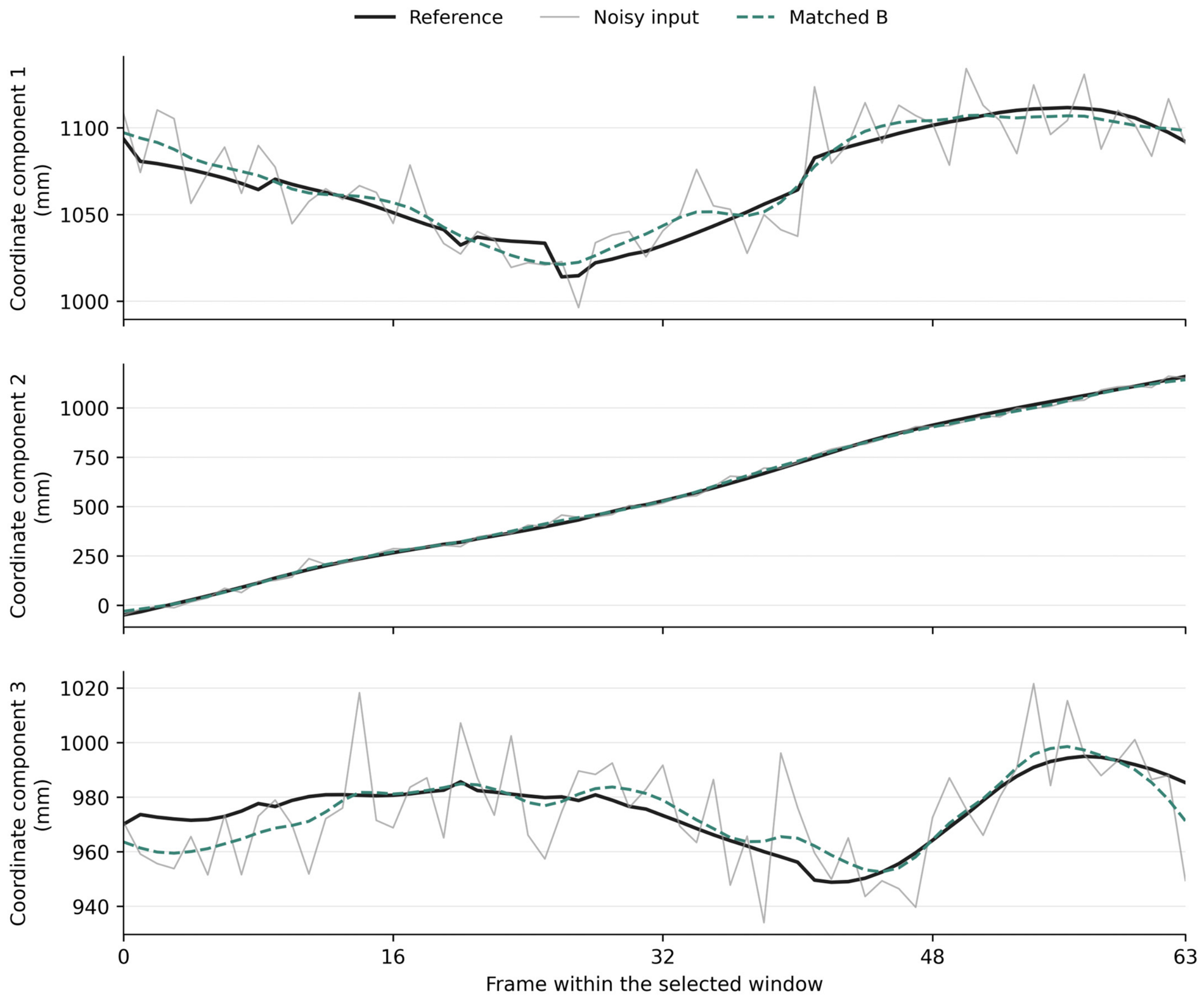
References
- Pavllo, D.; Feichtenhofer, C.; Grangier, D.; Auli, M. 3D human pose estimation in video with temporal convolutions and semi-supervised training. In Proceedings of the IEEE/CVF Conference on Computer Vision and Pattern Recognition (CVPR), Long Beach, CA, USA, 15–20 June 2019; pp. 7753–7762. [Google Scholar] [CrossRef] [Scilit]
- Li, W.; Liu, H.; Ding, R.; Liu, M.; Wang, P.; Yang, W. Exploiting temporal contexts with strided transformer for 3D human pose estimation. IEEE Trans. Multimed. 2023, 25, 1282–1293. [Google Scholar] [CrossRef] [Scilit]
- Zhang, J.; Tu, Z.; Yang, J.; Chen, Y.; Yuan, J. MixSTE: Seq2seq mixed spatio-temporal encoder for 3D human pose estimation in video. In Proceedings of the IEEE/CVF Conference on Computer Vision and Pattern Recognition (CVPR), New Orleans, LA, USA, 18–24 June 2022; pp. 13232–13242. [Google Scholar] [CrossRef] [Scilit]
- Mehraban, S.; Adeli, V.; Taati, B. MotionAGFormer: Enhancing 3D human pose estimation with a transformer-GCNFormer network. In Proceedings of the IEEE/CVF Winter Conference on Applications of Computer Vision (WACV), Waikoloa, HI, USA, 3–8 January 2024; pp. 6920–6930. [Google Scholar] [CrossRef] [Scilit]
- Zhao, Q.; Zheng, C.; Liu, M.; Wang, P.; Chen, C. PoseFormerV2: Exploring frequency domain for efficient and robust 3D human pose estimation. In Proceedings of the IEEE/CVF Conference on Computer Vision and Pattern Recognition (CVPR), Vancouver, BC, Canada, 17–24 June 2023; pp. 8877–8886. [Google Scholar] [CrossRef] [Scilit]
- Zheng, K.; Lu, F.; Lv, Y.; Zhang, L.; Guo, C.; Wu, J. 3D Human Pose Estimation via Non-Causal Retentive Networks. In European Conference on Computer Vision; Springer Nature Switzerland: Cham, Switzerland, 2024; pp. 111–128. [Google Scholar] [CrossRef] [Scilit]
- Wei, F.; Xu, G.; Wu, Q.; Qin, P.; Tian, P.; Pan, L.; Zhao, Y. Seq2seq motion continuity and limb invariance constrained spatial–temporal encoder for 3D human pose estimation. iScience 2025, 28, 114094. [Google Scholar] [CrossRef] [Scilit] [PubMed]
- Pham, Y.; Yuan, X.; Zhuang, C. Motion-Aware Graph Fusion Network for 3D Human Pose Estimation. In Proceedings of the IEEE/CVF Winter Conference on Applications of Computer Vision (WACV), Tucson, AZ, USA, 6–10 March 2026; pp. 5798–5808. [Google Scholar] [CrossRef] [Scilit]
- Chen, S.; Xu, Y.; Pu, Z.; Ouyang, J.; Zou, B. SkeletonPose: Exploiting human skeleton constraint for 3D human pose estimation. Knowl.-Based Syst. 2022, 255, 109691. [Google Scholar] [CrossRef] [Scilit]
- Ma, X.; Su, J.; Wang, C.; Ci, H.; Wang, Y. Context modeling in 3D human pose estimation: A unified perspective. In Proceedings of the IEEE/CVF Conference on Computer Vision and Pattern Recognition (CVPR), Nashville, TN, USA, 20–25 June 2021; pp. 6238–6247. [Google Scholar] [CrossRef] [Scilit]
- Gärtner, E.; Andriluka, M.; Xu, H.; Sminchisescu, C. Trajectory optimization for physics-based reconstruction of 3D human pose from monocular video. In Proceedings of the IEEE/CVF Conference on Computer Vision and Pattern Recognition (CVPR), New Orleans, LA, USA, 18–24 June 2022; pp. 13106–13115. [Google Scholar] [CrossRef] [Scilit]
- Du, S.; Yuan, Z.; Ikenaga, T. Kinematics-aware spatial-temporal feature transform for 3D human pose estimation. Pattern Recognit. 2024, 150, 110316. [Google Scholar] [CrossRef] [Scilit]
- Sun, X.; Shang, J.; Liang, S.; Wei, Y. Compositional human pose regression. In Proceedings of the IEEE International Conference on Computer Vision (ICCV), Venice, Italy, 22–29 October 2017; pp. 2602–2611. [Google Scholar] [CrossRef] [Scilit]
- Cao, X.; Zhao, X. Anatomy and geometry constrained one-stage framework for 3D human pose estimation. In Asian Conference on Computer Vision; Springer International Publishing: Cham, Switzerland, 2020; pp. 227–243. [Google Scholar] [CrossRef] [Scilit]
- Zeng, A.; Yang, L.; Ju, X.; Li, J.; Wang, J.; Xu, Q. SmoothNet: A plug-and-play network for refining human poses in videos. In European Conference on Computer Vision; Springer Nature Switzerland: Cham, Switzerland, 2022; pp. 625–642. [Google Scholar] [CrossRef] [Scilit]
- Zeng, A.; Ju, X.; Yang, L.; Gao, R.; Zhu, X.; Dai, B.; Xu, Q. DeciWatch: A simple baseline for 10× efficient 2D and 3D pose estimation. In European Conference on Computer Vision; Springer Nature Switzerland: Cham, Switzerland, 2022; pp. 607–624. [Google Scholar] [CrossRef] [Scilit]
- Liu, B.; Wang, H. PoseRL-Net: Human pose analysis for motion training guided by robot vision. Front. Neurorobot. 2025, 19, 1531894. [Google Scholar] [CrossRef] [Scilit] [PubMed]
- Liu, X.; Tang, H. BCDPose: Diffusion-based 3D Human Pose Estimation with bone-chain prior knowledge. Image Vis. Comput. 2025, 162, 105636. [Google Scholar] [CrossRef] [Scilit]
- Memon, A.; Arain, Q.; Manjotho, A.A.; Alanazi, M.H.; Uddin, M.; Shorfuzzaman, M. PosePerfect: Refining 3D human pose estimation using anthropometric constraints and synthetic localization errors. Vis. Comput. 2026, 42, 40. [Google Scholar] [CrossRef] [Scilit]
- Jiang, J.; Jian, Z.; Zheng, H.; Liang, M.; Shi, Y.; Zhang, L. HADD: A hierarchy-aware disentangled diffusion framework with spatio-temporal denoising for 3D human pose estimation. PLoS ONE 2026, 21, e0359321. [Google Scholar] [CrossRef] [Scilit] [PubMed]
- Sun, Z.; Liang, Y.; Ma, Z.; Zhang, T.; Bao, L.; Li, G.; He, S. RePOSE: 3D Human Pose Estimation via Spatio-Temporal Depth Relational Consistency. In European Conference on Computer Vision; Springer Nature Switzerland: Cham, Switzerland, 2024; pp. 309–325. [Google Scholar] [CrossRef] [Scilit]
- Davoodnia, V.; Ghorbani, S.; Carbonneau, M.-A.; Messier, A.; Etemad, A. UPose3D: Uncertainty-Aware 3D Human Pose Estimation with Cross-View and Temporal Cues. In European Conference on Computer Vision; Springer Nature Switzerland: Cham, Switzerland, 2024; pp. 19–38. [Google Scholar] [CrossRef] [Scilit]
- Zheng, H.; Li, H.; Dai, W.; Zheng, Z.; Li, C.; Zou, J.; Xiong, H. HiPART: Hierarchical Pose AutoRegressive Transformer for Occluded 3D Human Pose Estimation. In Proceedings of the IEEE/CVF Conference on Computer Vision and Pattern Recognition (CVPR), Nashville, TN, USA, 10–17 June 2025; pp. 16807–16817. [Google Scholar] [CrossRef] [Scilit]
- Xu, J.; Guo, Y.; Peng, Y. FinePOSE: Fine-Grained Prompt-Driven 3D Human Pose Estimation via Diffusion Models. In Proceedings of the IEEE/CVF Conference on Computer Vision and Pattern Recognition (CVPR), Seattle, WA, USA, 16–22 June 2024; pp. 561–570. [Google Scholar] [CrossRef] [Scilit]
- Zhang, S.; Bhatnagar, B.L.; Xu, Y.; Winkler, A.; Kadlecek, P.; Tang, S.; Bogo, F. RoHM: Robust Human Motion Reconstruction via Diffusion. In Proceedings of the IEEE/CVF Conference on Computer Vision and Pattern Recognition (CVPR), Seattle, WA, USA, 16–22 June 2024; pp. 14606–14617. [Google Scholar] [CrossRef] [Scilit]
- Hoang, T.-H.; Zehni, M.; Phan, H.; Vo, D.M.; Do, M.N. Improving the Robustness of 3D Human Pose Estimation: A Benchmark Dataset and Learning from Noisy Input. In Proceedings of the IEEE/CVF Conference on Computer Vision and Pattern Recognition Workshops (CVPRW), Seattle, WA, USA, 16–22 June 2024; pp. 113–123. [Google Scholar] [CrossRef] [Scilit]
- Magee, D.J. Orthopedic Physical Assessment, 6th ed.; Elsevier: St. Louis, MO, USA, 2013. [Google Scholar]
- Kingma, D.P.; Ba, J. Adam: A method for stochastic optimization. In Proceedings of the 3rd International Conference on Learning Representations (ICLR), San Diego, CA, USA, 7–9 May 2015. [Google Scholar]
- Loshchilov, I.; Hutter, F. SGDR: Stochastic gradient descent with warm restarts. In Proceedings of the 5th International Conference on Learning Representations (ICLR), Toulon, France, 24–26 April 2017. [Google Scholar]
- Ionescu, C.; Papava, D.; Olaru, V.; Sminchisescu, C. Human3.6M: Large scale datasets and predictive methods for 3D human sensing in natural environments. IEEE Trans. Pattern Anal. Mach. Intell. 2014, 36, 1325–1339. [Google Scholar] [CrossRef] [Scilit] [PubMed]
- Sener, O.; Koltun, V. Multi-task learning as multi-objective optimization. Adv. Neural Inf. Process. Syst. 2018, 31, 525–536. [Google Scholar]
- Lin, X.; Zhen, H.-L.; Li, Z.; Zhang, Q.-F.; Kwong, S. Pareto multi-task learning. Adv. Neural Inf. Process. Syst. 2019, 32, 12037–12047. [Google Scholar]
- Flash, T.; Hogan, N. The coordination of arm movements: An experimentally confirmed mathematical model. J. Neurosci. 1985, 5, 1688–1703. [Google Scholar] [CrossRef] [Scilit] [PubMed]
- Chen, T.; Fang, C.; Shen, X.; Zhu, Y.; Chen, Z.; Luo, J. Anatomy-aware 3D human pose estimation with bone-based pose decomposition. IEEE Trans. Circuits Syst. Video Technol. 2022, 32, 198–209. [Google Scholar] [CrossRef] [Scilit]
- Hsu, C.-H.; Jang, J.-S.R. Enhancing 3D human pose estimation with bone length adjustment. In Asian Conference on Computer Vision; Springer Nature Singapore: Singapore, 2024; pp. 242–257. [Google Scholar] [CrossRef] [Scilit]
- Kendall, A.; Gal, Y.; Cipolla, R. Multi-task learning using uncertainty to weigh losses for scene geometry and semantics. In Proceedings of the IEEE/CVF Conference on Computer Vision and Pattern Recognition (CVPR), Salt Lake City, UT, USA, 18–22 June 2018; pp. 7482–7491. [Google Scholar] [CrossRef] [Scilit]
- Chen, Z.; Badrinarayanan, V.; Lee, C.-Y.; Rabinovich, A. GradNorm: Gradient normalization for adaptive loss balancing in deep multitask networks. In Proceedings of the 35th International Conference on Machine Learning (ICML), Stockholm, Sweden, 10–15 July 2018; pp. 794–803. [Google Scholar]
- Akhter, I.; Black, M.J. Pose-conditioned joint angle limits for 3D human pose reconstruction. In Proceedings of the IEEE Conference on Computer Vision and Pattern Recognition (CVPR), Boston, MA, USA, 7–12 June 2015; pp. 1446–1455. [Google Scholar] [CrossRef] [Scilit]
- Bogo, F.; Kanazawa, A.; Lassner, C.; Gehler, P.; Romero, J.; Black, M.J. Keep it SMPL: Automatic estimation of 3D human pose and shape from a single image. In European Conference on Computer Vision; Springer: Cham, Switzerland, 2016; pp. 561–578. [Google Scholar] [CrossRef] [Scilit]
- Mehta, D.; Rhodin, H.; Casas, D.; Fua, P.; Sotnychenko, O.; Xu, W.; Theobalt, C. Monocular 3D human pose estimation in the wild using improved CNN supervision. In Proceedings of the International Conference on 3D Vision (3DV), Qingdao, China, 10–12 October 2017; pp. 506–516. [Google Scholar] [CrossRef] [Scilit]
- von Marcard, T.; Henschel, R.; Black, M.J.; Rosenhahn, B.; Pons-Moll, G. Recovering accurate 3D human pose in the wild using IMUs and a moving camera. In European Conference on Computer Vision (ECCV); Springer: Cham, Switzerland, 2018; pp. 601–617. [Google Scholar] [CrossRef] [Scilit]
- Mahmood, N.; Ghorbani, N.; Troje, N.F.; Pons-Moll, G.; Black, M.J. AMASS: Archive of motion capture as surface shapes. In Proceedings of the IEEE/CVF International Conference on Computer Vision (ICCV), Seoul, Republic of Korea, 27 October–2 November 2019; pp. 5442–5451. [Google Scholar] [CrossRef] [Scilit]
- Kocabas, M.; Huang, C.-H.P.; Hilliges, O.; Black, M.J. PARE: Part attention regressor for 3D human body estimation. In Proceedings of the IEEE/CVF International Conference on Computer Vision (ICCV), Montreal, QC, Canada, 10–17 October 2021; pp. 11107–11117. [Google Scholar] [CrossRef] [Scilit]
- Rempe, D.; Birdal, T.; Hertzmann, A.; Yang, J.; Sridhar, S.; Guibas, L.J. HuMoR: 3D human motion model for robust pose estimation. In Proceedings of the IEEE/CVF International Conference on Computer Vision (ICCV), Montreal, QC, Canada, 10–17 October 2021; pp. 11468–11479. [Google Scholar] [CrossRef] [Scilit]
- Kolotouros, N.; Pavlakos, G.; Black, M.J.; Daniilidis, K. Learning to reconstruct 3D human pose and shape via model-fitting in the loop. In Proceedings of the IEEE/CVF International Conference on Computer Vision (ICCV), Seoul, Republic of Korea, 27 October–2 November 2019; pp. 2252–2261. [Google Scholar] [CrossRef] [Scilit]
- Kocabas, M.; Athanasiou, N.; Black, M.J. VIBE: Video inference for human body pose and shape estimation. In Proceedings of the IEEE/CVF Conference on Computer Vision and Pattern Recognition (CVPR), Seattle, WA, USA, 13–19 June 2020; pp. 5253–5263. [Google Scholar] [CrossRef] [Scilit]
- Wang, J.; Cao, Z.; Luvizon, D.; Liu, L.; Sarkar, K.; Tang, D.; Beeler, T.; Theobalt, C. Egocentric Whole-Body Motion Capture with FisheyeViT and Diffusion-Based Motion Refinement. In Proceedings of the IEEE/CVF Conference on Computer Vision and Pattern Recognition (CVPR), Seattle, WA, USA, 16–22 June 2024; pp. 777–787. [Google Scholar] [CrossRef] [Scilit]
- Stathopoulos, A.; Han, L.; Metaxas, D. Score-Guided Diffusion for 3D Human Recovery. In Proceedings of the IEEE/CVF Conference on Computer Vision and Pattern Recognition (CVPR), Seattle, WA, USA, 16–22 June 2024; pp. 906–915. [Google Scholar] [CrossRef] [Scilit]
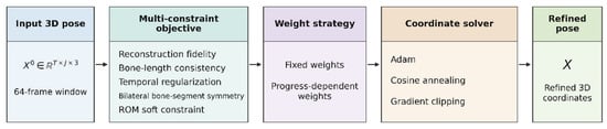
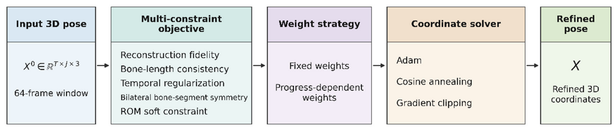
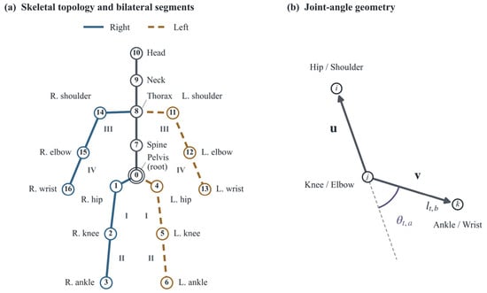
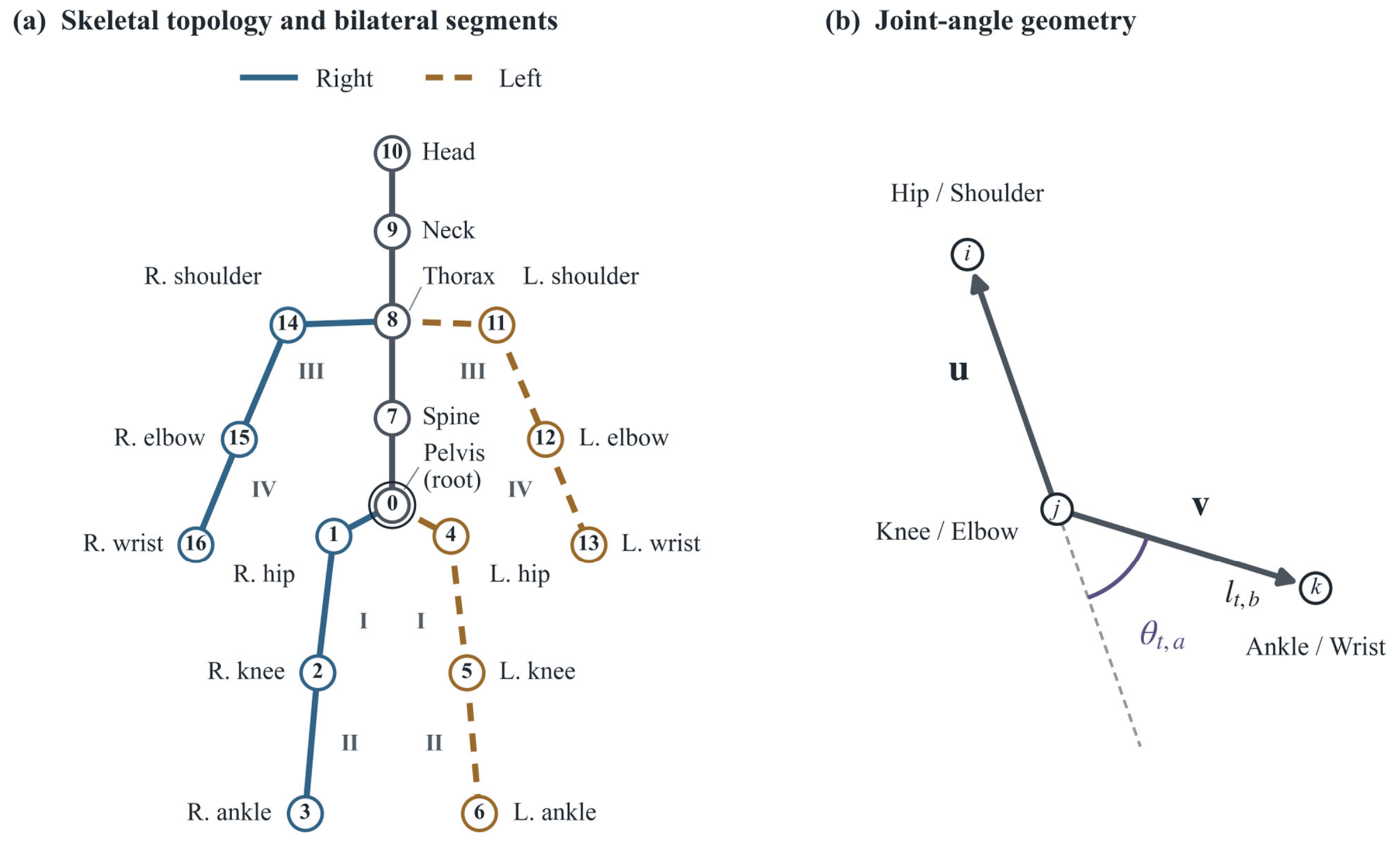
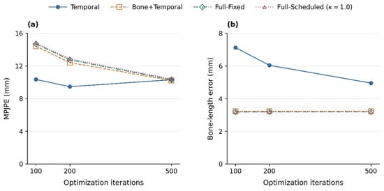
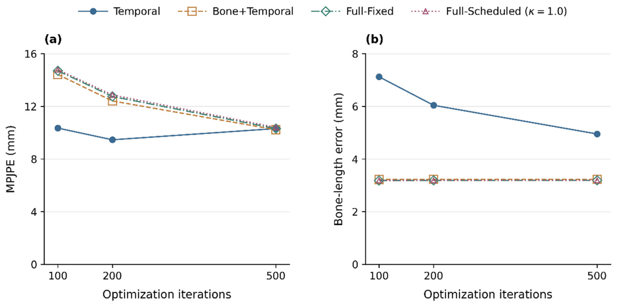
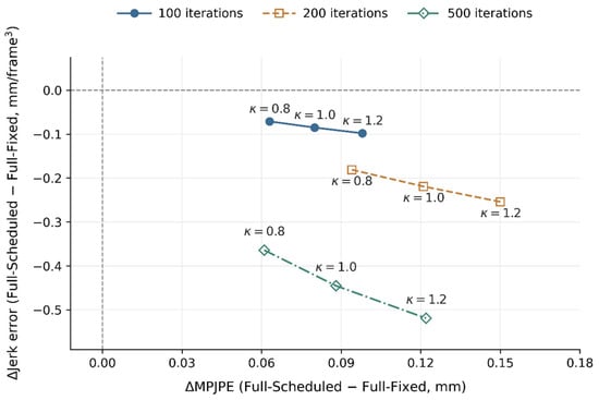
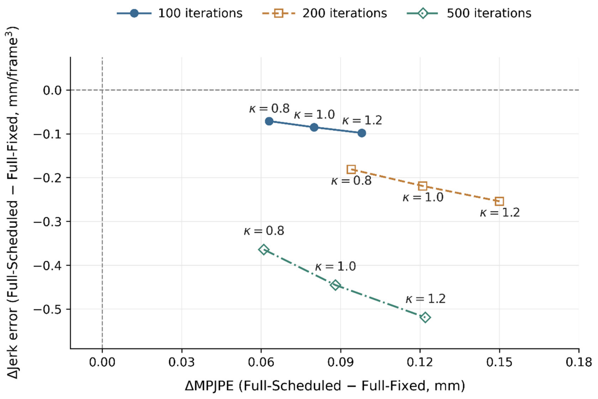
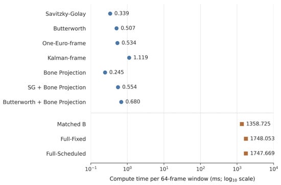
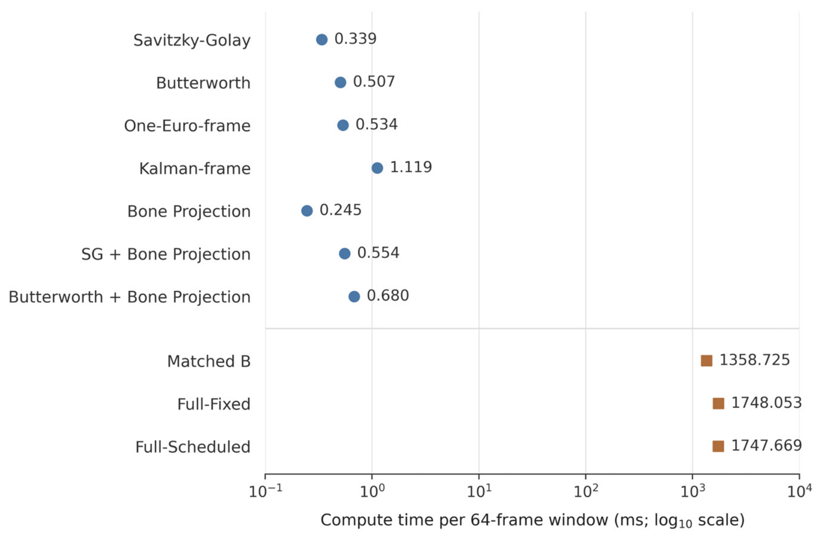
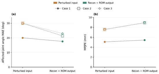
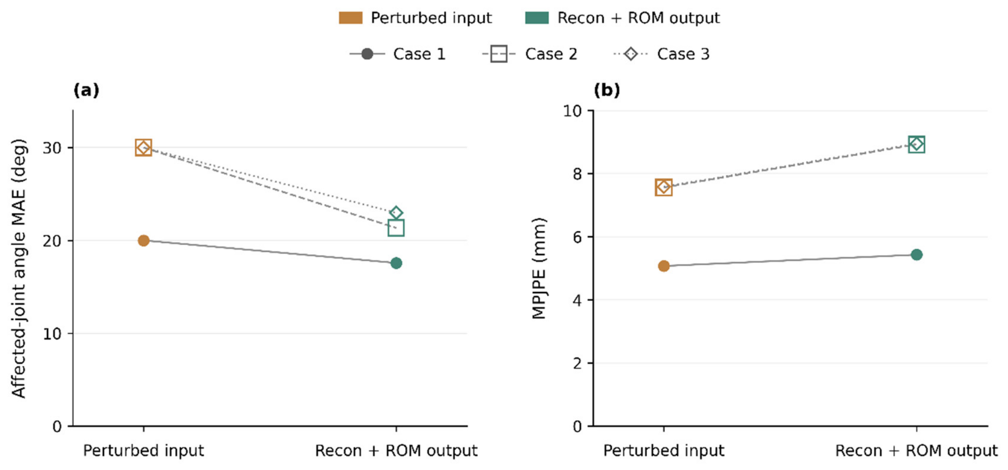
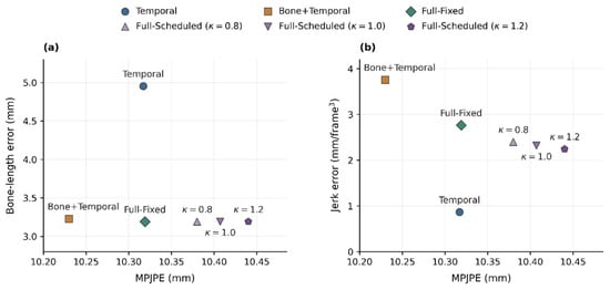
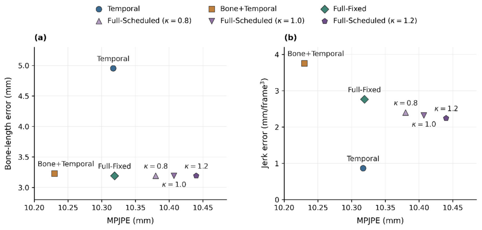
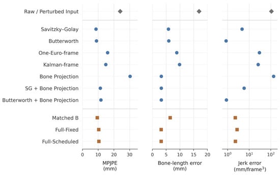
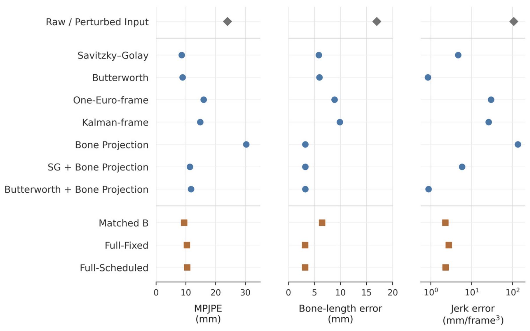
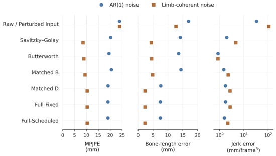
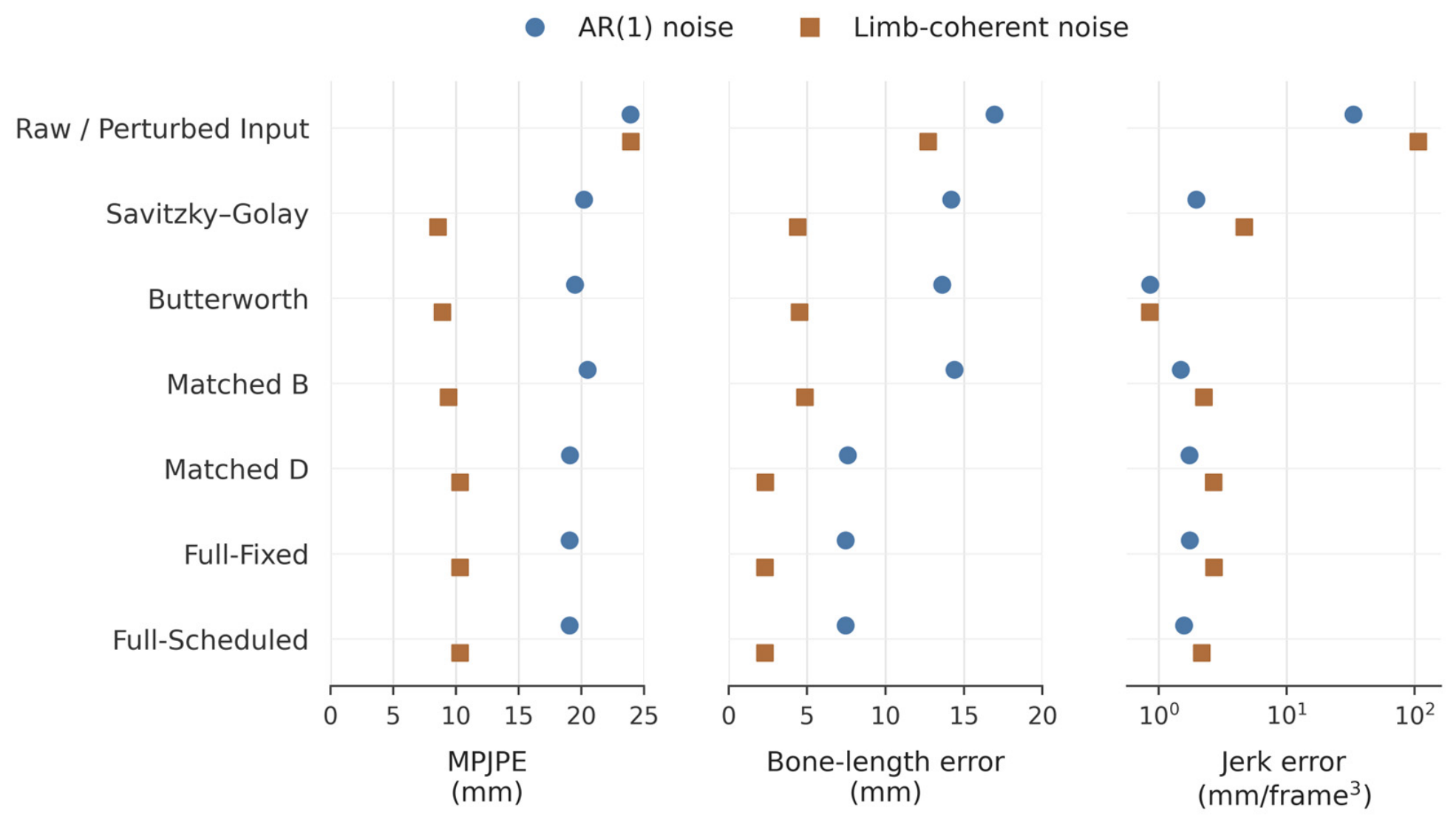
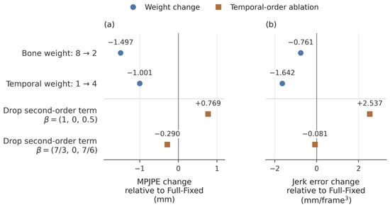
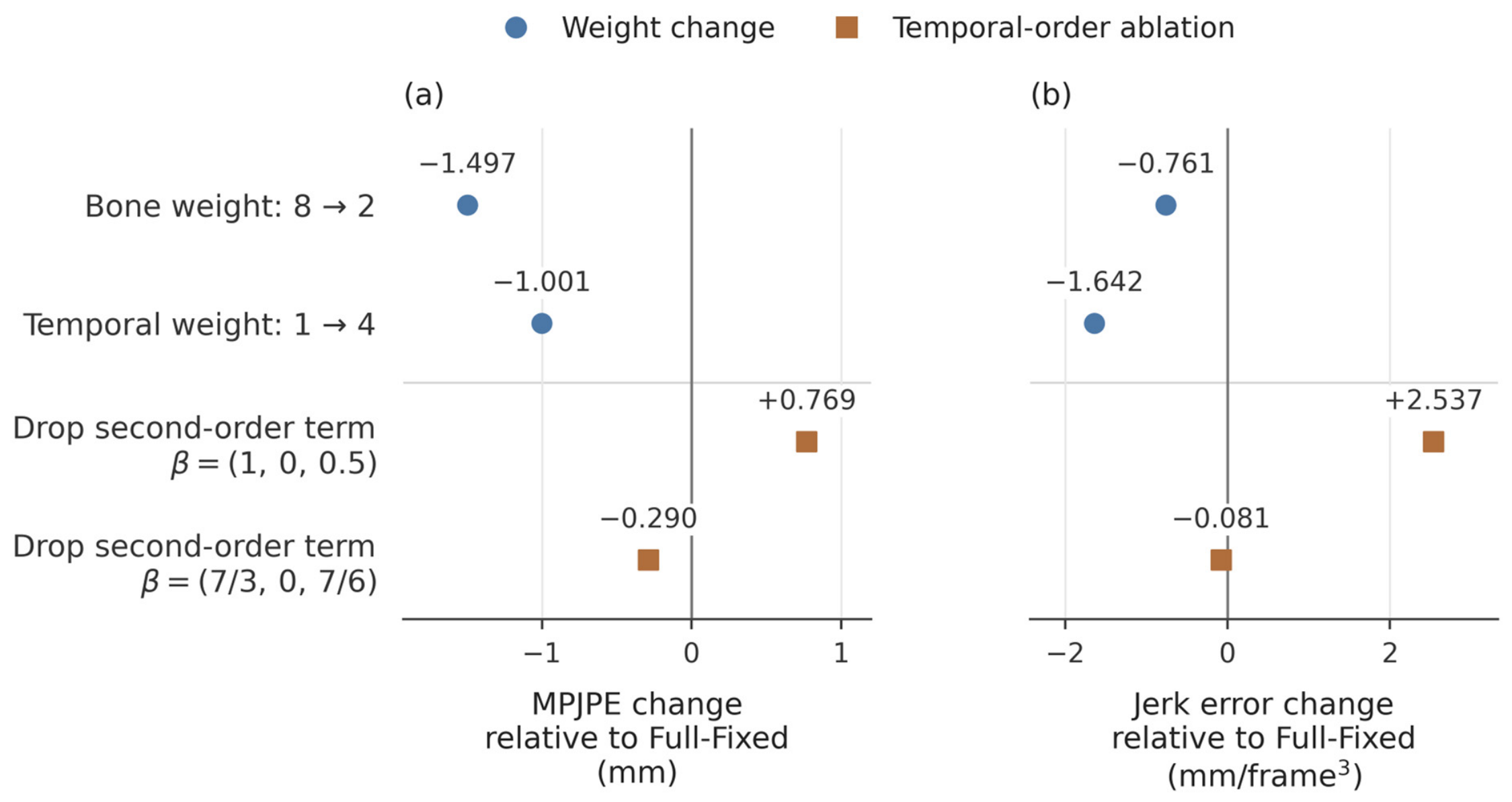
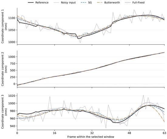
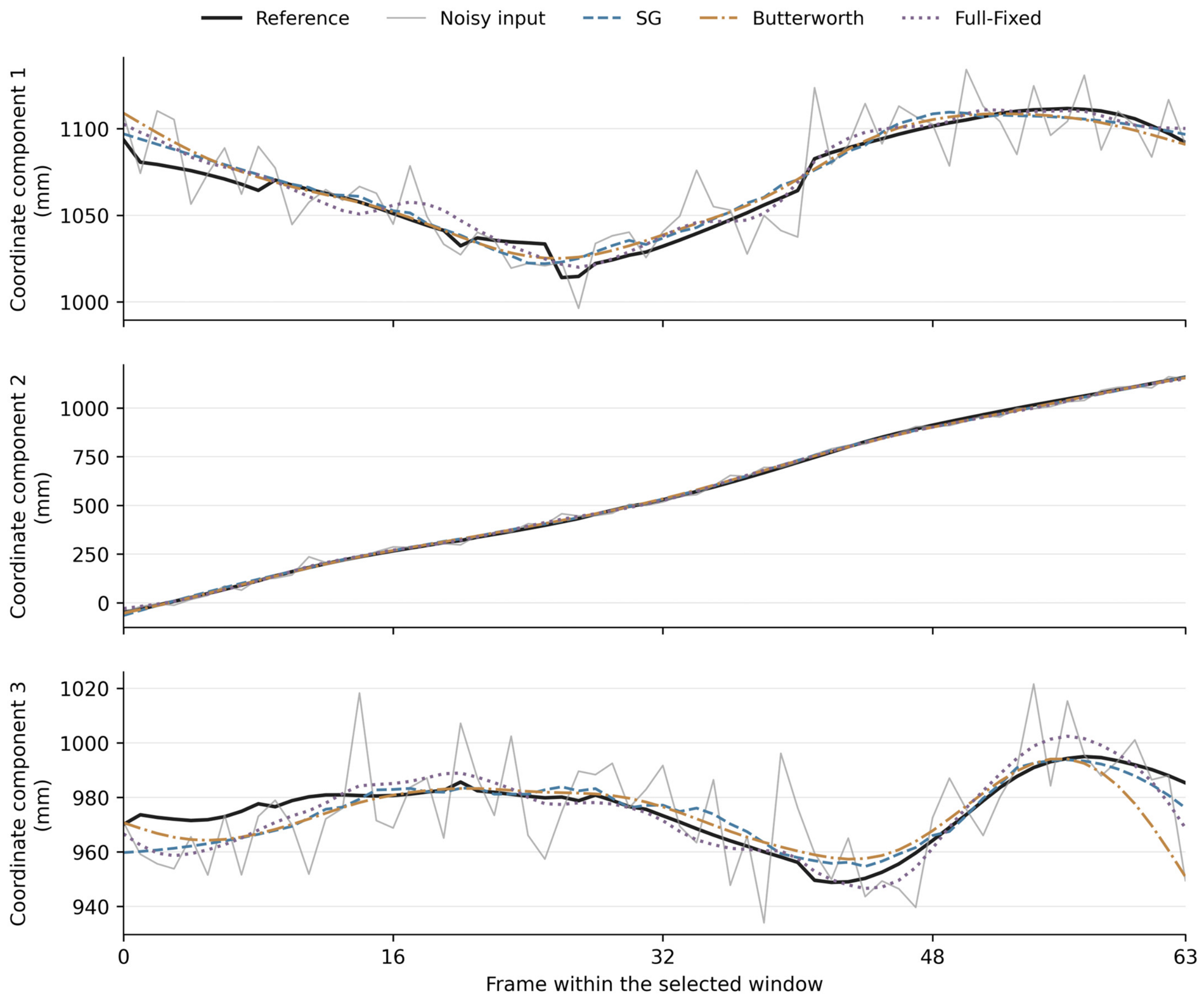
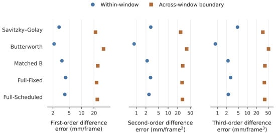
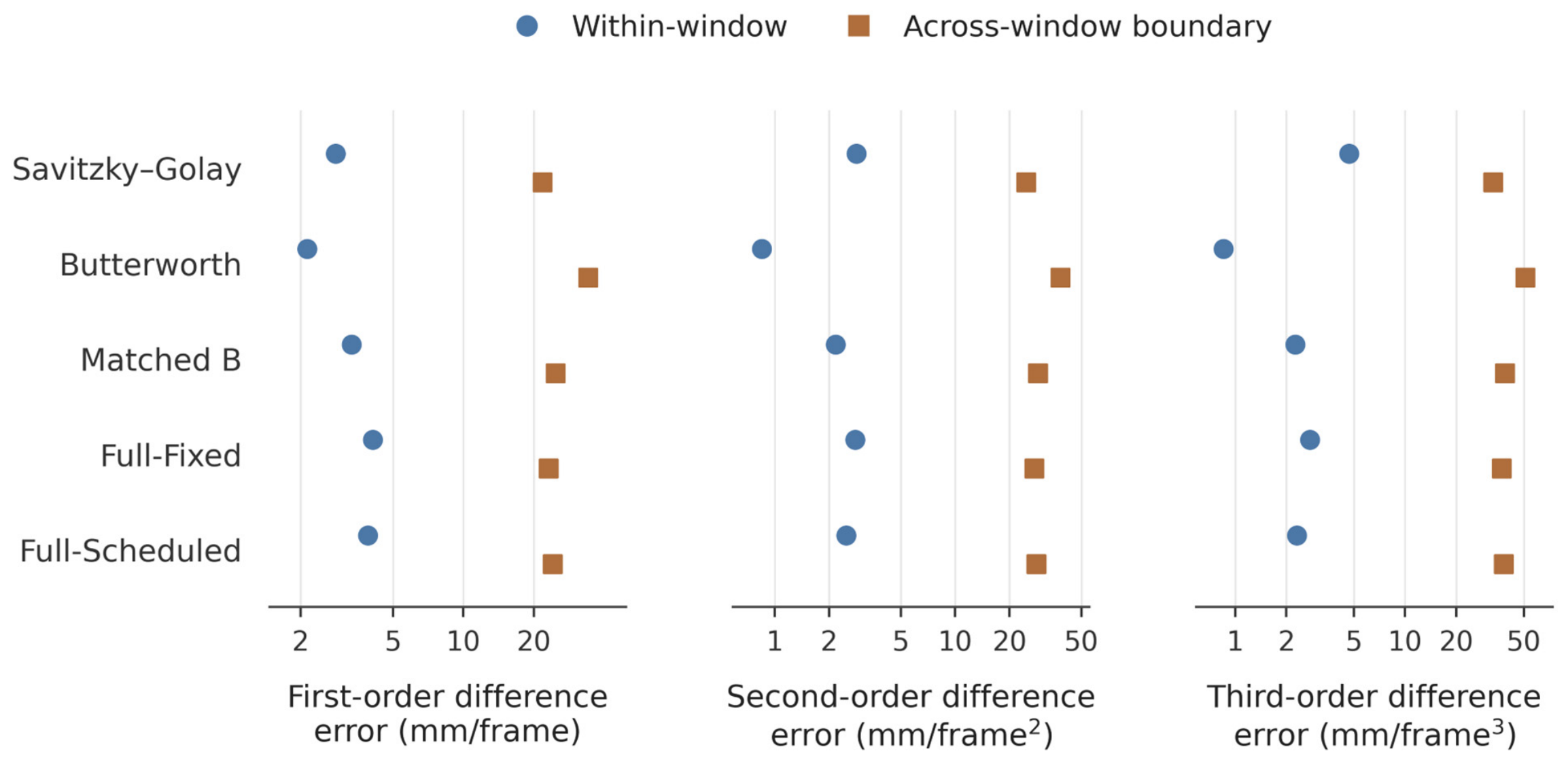
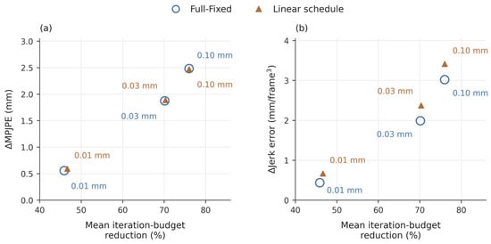
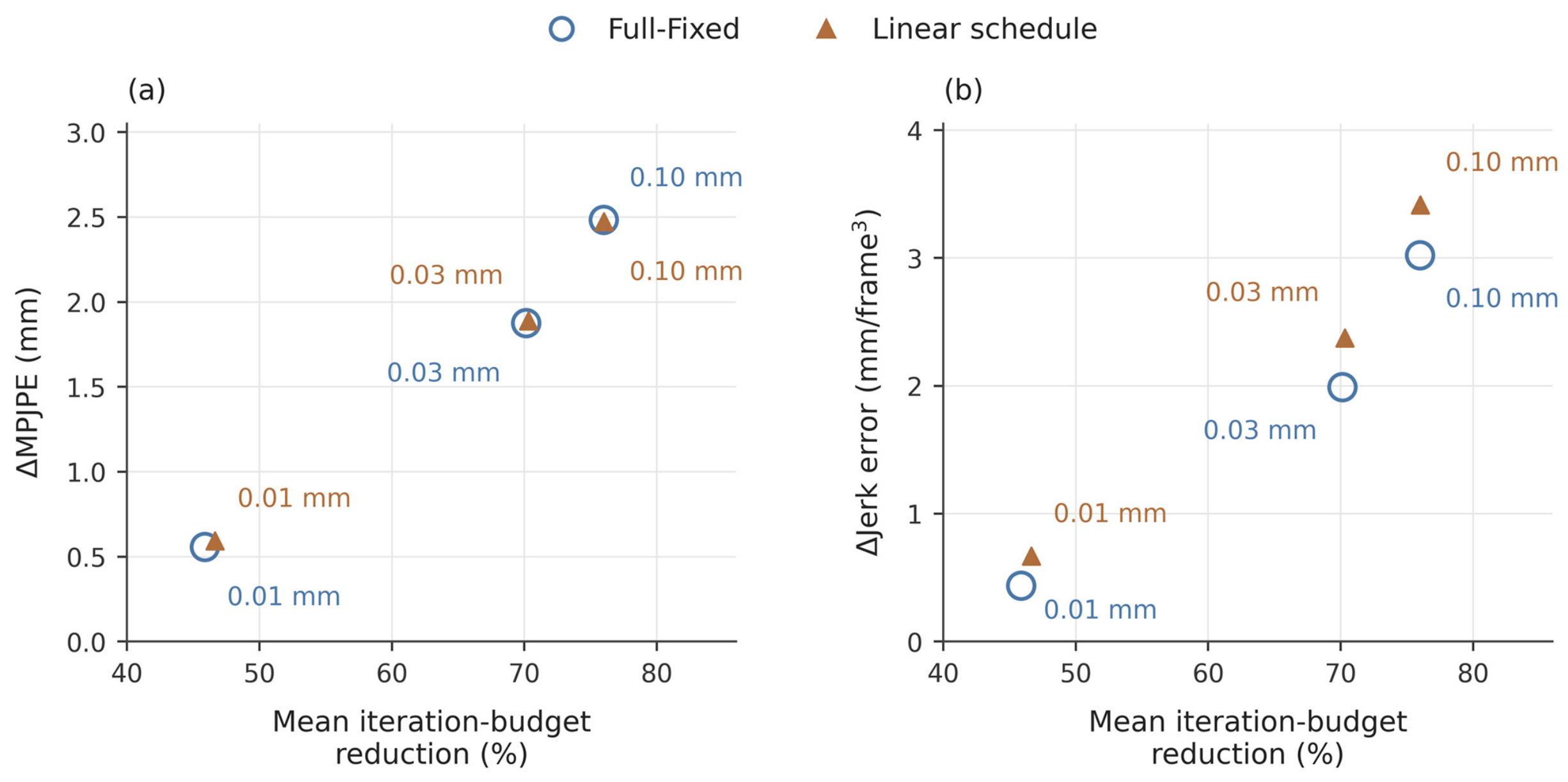

Disclaimer/Publisher’s Note: The statements, opinions and data contained in all publications are solely those of the individual author(s) and contributor(s) and not of MDPI and/or the editor(s). MDPI and/or the editor(s) disclaim responsibility for any injury to people or property resulting from any ideas, methods, instructions or products referred to in the content. |
© 2026 by the authors. Licensee MDPI, Basel, Switzerland. This article is an open access article distributed under the terms and conditions of the Creative Commons Attribution (CC BY) license.