Lightweight LSTM-Enhanced In-Flight Alignment for SINS/GPS Integrated Navigation

Abstract

Accurate in-flight alignment of strapdown inertial navigation systems (SINSs) is essential for reliable navigation under dynamic conditions. However, conventional SINS/GPS Kalman filtering (KF) is susceptible to model inaccuracies, uncertain noise statistics, and GPS outages, which may degrade alignment performance. To address these challenges, this paper proposes a lightweight KF–LSTM collaborative alignment method based on GPS measurement availability. Under normal GPS conditions, a long short-term memory (LSTM) network extracts temporal features from historical SINS/GPS position and velocity differences to refine KF misalignment angle estimates through output-level correction. During GPS outages, an independently trained LSTM generates misalignment-angle pseudo-measurements using inertial measurements and predicted navigation error states to assist KF updates. Upon GPS recovery, conventional measurement updates are resumed, followed by reactivation of the output-level correction mechanism. A lightweight LSTM architecture is selected based on accuracy–complexity analysis. Simulation and vehicle experiments are conducted to evaluate the proposed method against conventional and learning-assisted filtering approaches. The results demonstrate the feasibility of the proposed collaborative framework and its potential to improve alignment performance under varying GPS conditions.

1. Introduction

The strapdown inertial navigation system (SINS) continuously provides attitude, velocity, and position information by integrating angular velocity and specific force measurements from inertial sensors. Owing to its autonomy, high update rate, and continuous navigation capability, SINS has been widely employed in aerospace systems and unmanned aerial vehicles. Initial alignment is essential for establishing the attitude relationship between the body frame and the navigation frame. For aircraft requiring rapid deployment or navigation system reinitialization during flight, conventional stationary alignment methods are often impractical, making in-flight alignment particularly important. Wu and Pan [1] developed a velocity/position integration approach for in-flight coarse alignment using GPS measurements. Lu et al. [2] proposed an improved in-flight alignment method for low-cost SINS/GPS integrated navigation systems, while Ning et al. [3] investigated a robust position integration optimization method to improve in-flight coarse alignment. Despite these developments, alignment performance remains affected by inertial sensor errors, complex vehicle maneuvers, and the availability of external navigation observations.

Kalman filtering (KF) is widely adopted in SINS/GPS integrated navigation to estimate misalignment angles, velocity and position errors, and inertial sensor biases. By incorporating GPS position and velocity measurements, the KF recursively estimates and compensates for accumulated inertial navigation errors. However, its performance depends on the accuracy of the system model and the assumed noise statistics. Under complex maneuvering conditions or varying GPS measurement quality, model mismatch and inaccurate noise covariance information may degrade estimation accuracy. To address these limitations, Mohamed and Schwarz [4] developed an innovation-based adaptive Kalman filtering approach for INS/GPS integration. Liu et al. [5] further proposed an adaptive information fusion method to improve navigation performance under uncertain noise conditions. Although adaptive filtering techniques can enhance estimation performance, their effectiveness depends on appropriate covariance adaptation strategies. Moreover, when valid GPS observations are completely unavailable, measurement-based correction cannot be maintained using conventional GPS updates.

With advances in data-driven modeling, neural networks have increasingly been incorporated into INS/GNSS integrated navigation systems to capture nonlinear relationships and temporal characteristics that are difficult to represent using conventional error models. Sharaf et al. [6] investigated radial basis function neural networks for online INS/GPS integration. Noureldin et al. [7] employed dynamic neural networks to exploit historical navigation information for vehicular navigation. Subsequently, Dai et al. [8] introduced a recurrent neural network (RNN)-based INS/GNSS integration method to predict inertial navigation errors in GNSS-denied environments. Sun et al. [9] further investigated a machine-learning-aided SINS/GPS integration approach for navigation during GPS outages. These studies demonstrated the feasibility of combining data-driven error estimation with conventional navigation algorithms. Nevertheless, the performance of learning-assisted methods depends on the selection of input features, prediction targets, network architectures, and information fusion strategies.

Long short-term memory (LSTM) networks, originally introduced by Hochreiter and Schmidhuber [10], can capture temporal dependencies through gated memory mechanisms, making them suitable for modeling the evolution of inertial navigation errors. Fang et al. [11] proposed an LSTM-based pseudo-measurement estimation algorithm that predicts GNSS position increments to assist inertial navigation during signal outages. In addition to LSTM, gated recurrent units (GRUs) have been investigated as an alternative architecture for temporal sequence modeling [12]. Tang et al. [13] developed a GRU- and adaptive Kalman filter-based hybrid algorithm to improve INS/GNSS integration during GNSS outages, while Zhao et al. [14] combined CNN–GRU networks with cubature Kalman filtering to predict navigation increments. Furthermore, Alaeiyan et al. [15] investigated incremental regularized LSTM learning to improve GPS/INS integration during measurement interruptions. These studies indicate that recurrent learning models can provide auxiliary navigation information when GNSS observations are unavailable, although their prediction accuracy and computational requirements depend on the network design and operating conditions.

More recently, increasing attention has been directed toward learning-based pseudo-measurement generation and hybrid neural network–filtering frameworks. Wang et al. [16] developed a Cascade-LSTM-based pseudo-velocity measurement method for bridging GNSS outages, in which learned navigation information is incorporated into Kalman filtering. Dai et al. [17] proposed a CNN–BiLSTM–attention architecture to improve integrated navigation accuracy under GNSS-denied conditions. Niu et al. [18] further investigated a TCN–BiLSTM and adaptive filtering framework for maintaining vehicle positioning during GNSS outages. In addition, Sahoo and Klein [19] introduced physics-informed learning for pure inertial navigation without external positioning observations. These developments demonstrate the growing diversity of learning-assisted navigation approaches, ranging from error prediction and pseudo-observation reconstruction to hybrid model-based and data-driven estimation.

Despite these advances, several challenges remain in applying learning-assisted estimation to SINS/GPS in-flight alignment. First, existing learning-based INS/GNSS integration methods have predominantly focused on position and velocity error compensation or the reconstruction of unavailable GNSS-related observations, whereas the estimation of three-axis misalignment angles during dynamic alignment requires a different prediction objective and measurement formulation. Second, the relationship between neural network predictions and KF state estimates must be explicitly defined to ensure consistent information fusion. In particular, directly incorporating auxiliary predictions into the KF under normal GPS conditions may complicate the measurement update process, while using historical SINS/GPS differences as network inputs becomes infeasible when current GPS measurements are unavailable. Third, network complexity and prediction uncertainty must be considered to ensure that learning-assisted estimation remains suitable for resource-constrained navigation applications. Therefore, a collaborative estimation strategy that explicitly accounts for GPS measurement availability and assigns different roles to the learning model under normal and outage conditions warrants further investigation.

To address these issues, this paper proposes a lightweight KF–LSTM collaborative in-flight alignment method with GPS measurement availability-based mode switching. The proposed framework retains the KF as the primary state estimator while employing LSTM networks to extract temporal information for auxiliary misalignment angle estimation. Under normal GPS conditions, an LSTM network processes historical SINS/GPS position and velocity differences, and its predictions are incorporated through an output-level correction mechanism without modifying the internal GPS-based KF measurement update. During GPS outages, a separately trained LSTM uses inertial measurements and predicted navigation error states to generate three-axis misalignment-angle pseudo-measurements, which are incorporated into the KF through a dedicated measurement model. Following GPS recovery, conventional measurement updates are resumed, and output-level correction is reactivated after the required historical input sequence has been reconstructed. In addition, a lightweight LSTM architecture is selected through a sensitivity analysis of input window length and hidden-layer size, and its performance is evaluated against conventional KF, adaptive KF, KF–MLP, and KF–GRU methods. Unlike methods that primarily reconstruct unavailable GNSS position or velocity observations, the proposed approach focuses on misalignment-angle-oriented auxiliary estimation and mode-dependent collaboration between model-based filtering and temporal learning.

The remainder of this paper is organized as follows. Section 2 presents the SINS/GPS error-state model and GPS measurement availability detection method. Section 3 describes the lightweight LSTM architecture and the proposed KF–LSTM collaborative alignment strategy. Section 4 presents the simulation and experimental results. Finally, Section 5 concludes the paper.

2. The In-Flight Alignment System Design

2.1. Filter Model Configuration of SINS/GPS

The East–North–Up (ENU) coordinate system has been selected as the navigation coordinate system, and the error misalignment angle ϕⁿ, velocity error δVⁿ, position error δPⁿ, drift error of the gyroscope ${\mathit{\epsilon }}^{\mathit{b}}$ and accelerometer ${\mathit{\nabla }}^{\mathit{b}}$ of the SINS are selected as the state variables of the system:

$${\mathbf{X}}_{\mathit{k}}={\left[\begin{array}{lllll}{\mathit{\varphi }}^{\mathit{n}}\hfill & \delta {\mathit{V}}^{\mathit{n}}\hfill & \delta {\mathit{P}}^{\mathit{n}}\hfill & {\mathit{\epsilon }}^{\mathit{b}}\hfill & {\mathit{\nabla }}^{\mathit{b}}\hfill \end{array}\right]}^{\mathit{T}}$$

(1)

The state equation of the initial alignment in the integrated system can be written as follows:

$$\dot{\mathit{X}}(t)=\mathit{F}(t)\mathit{X}(t)+\mathit{G}(t)\mathit{W}(t)$$

(2)

where F(t) is the continuous-time system matrix, G(t) is the process noise distribution matrix, and W(t) denotes the process noise vector.

When valid GPS measurements are available, a six-dimensional observation vector is constructed using the position and velocity differences between GPS and SINS:

$${\mathit{Z}}_k=\left[\begin{array}{c}\Delta {\mathit{P}}_k\\ \Delta {\mathit{V}}_k\end{array}\right]=\left[\begin{array}{c}{\mathit{P}}_{\mathit{GPS},k}-{\mathit{P}}_{\mathit{SINS},k}\\ {\mathit{V}}_{\mathit{GPS},k}-{\mathit{V}}_{\mathit{SINS},k}\end{array}\right]$$

(3)

ΔP_k, ΔV_k represent the position and velocity differences between GPS and SINS, respectively. Considering GPS measurement noise, the observation equation can be written as

Z_k = H_kX_k + V_k

(4)

where H_k denotes the GPS observation matrix, and V_k is the GPS measurement noise vector. For discrete-time recursive estimation, Equation (2) is discretized as

X_k+1 = Φ_k+1,kX_k + W_k

(5)

where Φ_k+1,k denotes the discrete-time state transition matrix, and W_k represents the discrete process noise vector with covariance matrix Q_k.

As we all know, due to the continuous error accumulation of SINS, the positioning error of SINS will diverge rapidly. Because GPS can continuously provide high-precision location information, the integrated method is good for localization. However, the shortcomings of the integrated method are maintaining the accuracy of GPS in order to accomplish the in-flight alignment of the aircraft.

2.2. The Availability Determination of the GPS Signal

Firstly, we must determine whether the GPS signal is effective or not. The residual χ² detection method has been adopted to detect the signal of GPS. The innovation vector r_k, defined as the difference between the actual GPS measurement and its predicted value, is expressed as follows:

$${\mathit{r}}_k={\mathit{Z}}_k-{\mathit{H}}_k{\widehat{\mathit{X}}}_{k/k-1}$$

(6)

where ${\widehat{\mathit{X}}}_{k/k-1}$ denotes the prior state estimate at time step k, obtained by propagating the posterior state estimate from the previous time step through the system state transition model.

Under the assumed system model and noise statistics, the innovation vector approximately follows a zero-mean Gaussian distribution when the GPS measurements are valid. Its covariance matrix is expressed as

$${\mathit{S}}_k=={\mathit{H}}_k{\mathit{P}}_{k/k-1}{\mathit{H}}_k^T+{\mathit{R}}_k$$

(7)

where P_k/k−1 is the prior state estimation error covariance matrix, and R_k denotes the GPS measurement noise covariance matrix.

To evaluate the consistency between the GPS measurements and the predicted observations while accounting for their statistical uncertainties, the normalized innovation squared statistic is constructed as

$${\lambda }_k={\mathit{r}}_k^T{\mathit{S}}_k^{-1}{\mathit{r}}_k~{\chi }^2(m)$$

(8)

where m is the dimension of the GPS observation vector. Since the observation vector in this study consists of three-dimensional position differences and three-dimensional velocity differences, m = 6.

For a predefined false-alarm probability α, the detection threshold T_D is determined from the chi-square distribution as

$$T_D={\chi }_{6,1-\alpha }^2$$

(9)

where ${\chi }_{6,1-\alpha }^2$ denotes the quantile of the chi-square distribution with six degrees of freedom at a cumulative probability of 1 − α.

Provided that the GPS receiver supplies valid position and velocity measurements, the GPS measurement availability indicator is determined by comparing the detection statistic with the predefined threshold:

$$s_k=\left\{\begin{array}{c}1,{\lambda }_k\le T_D\\ 0,{\lambda }_k>T_D\end{array}\right.$$

(10)

where s_k denotes the GPS measurement availability indicator. When s_k is 1, the current GPS measurements pass the innovation consistency test and are accepted for the conventional SINS/GPS KF measurement update. Conversely, when s_k is 0, the measurements exhibit a statistically significant inconsistency with the predicted observations and are excluded from the KF measurement update.

3. Lightweight LSTM-Based KF–LSTM Collaborative In-Flight Alignment Method

3.1. Overall Architecture of the KF–LSTM Collaborative Alignment Method

In this section, a lightweight long short-term memory (LSTM) network is introduced to develop a KF–LSTM collaborative alignment method. The proposed method employs the Kalman filter (KF) as the primary state estimator, while the LSTM captures the temporal evolution characteristics of navigation errors to provide auxiliary corrections for misalignment angle estimation.

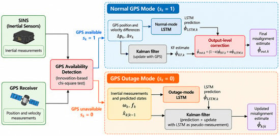
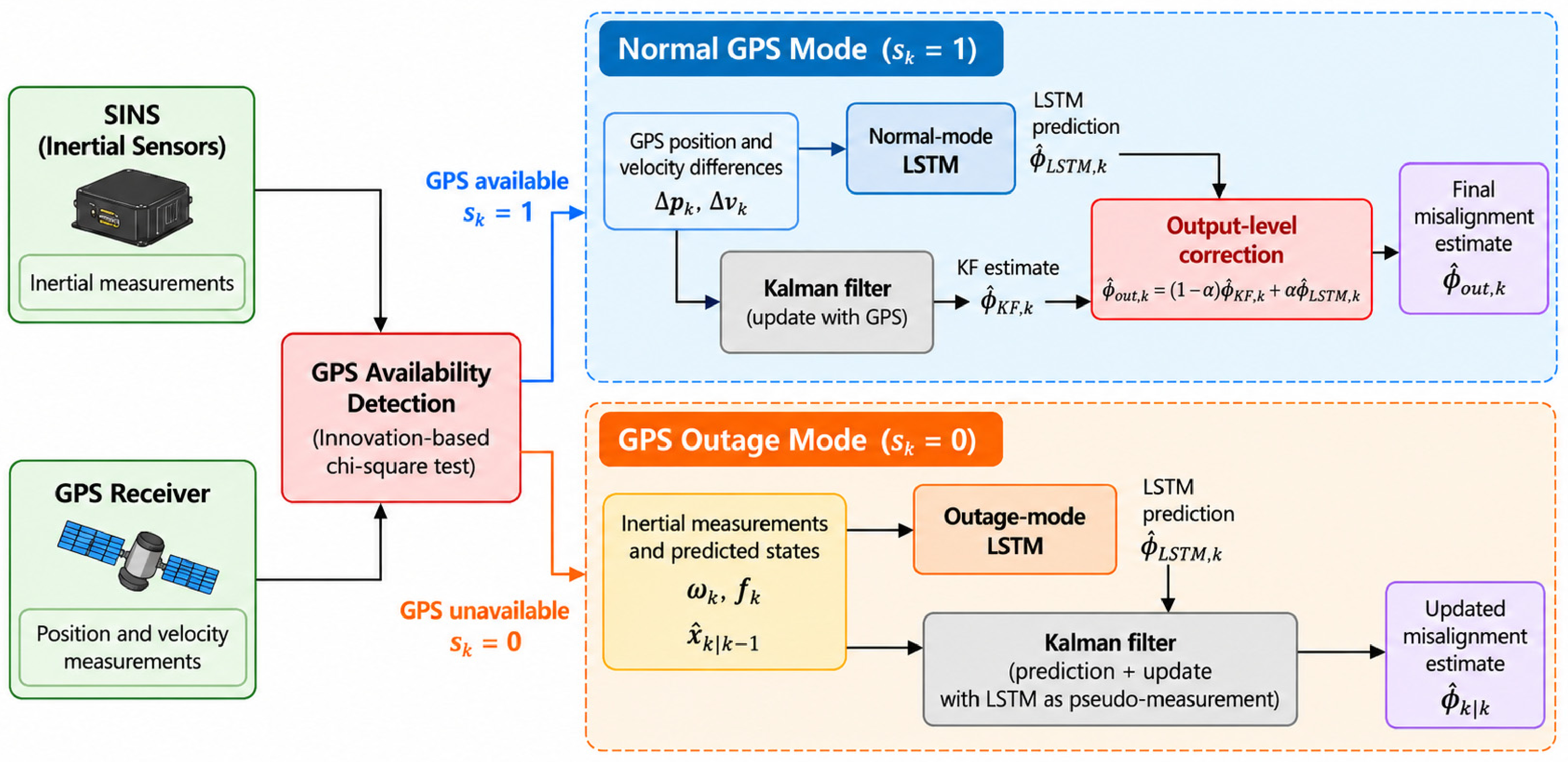
According to GPS measurement availability, the proposed method operates in three modes. In the GPS-available mode, the KF performs state estimation using GPS observations, while the LSTM improves the accuracy of misalignment angle estimation through an output-level correction mechanism. In the GPS-outage mode, the LSTM generates pseudo-measurements of the misalignment angles using inertial sensor measurements and predicted navigation error states, which are subsequently incorporated into the KF for auxiliary state updates. In the GPS-recovery mode, GPS-based measurement updates are resumed, and the output-level correction mechanism is reactivated once the historical input sequence required by the LSTM has been reconstructed.

Through this mode-switching mechanism, the proposed method enables collaborative state estimation between the KF and LSTM under varying GPS conditions. The overall architecture of the proposed KF–LSTM collaborative alignment method is illustrated in Figure 1.

Figure 1. Overall architecture of the proposed KF–LSTM collaborative alignment method with GPS availability-based mode switching.

3.2. LSTM Network Architecture and Parameter Configuration

Under normal GPS conditions, the position and velocity differences between SINS and GPS contain information related to the evolution of inertial navigation errors. Accordingly, a six-dimensional input vector u_k is constructed as

$${\mathit{u}}_k={\left[\begin{array}{cc}\Delta {\mathit{P}}_k^T& \Delta {\mathit{V}}_k^T\end{array}\right]}^T$$

(11)

where ΔP_k = P_GPS,k − P_SINS,k denotes the position differences of GPS and SINS, and ΔV_k = V_GPS,k − V_SINS,k denotes the velocity differences of GPS and SINS.

To capture the temporal characteristics of navigation errors, a sliding window containing (L) consecutive time steps is employed to construct the input sequence:

$${\mathit{U}}_k={\left[\begin{array}{ccc}{\tilde{\mathit{u}}}_{k-L+1}& \dots & {\tilde{\mathit{u}}}_k\end{array}\right]}^T$$

(12)

where ${\tilde{\mathit{u}}}_k$ represents the normalized input vector.

The LSTM learns the temporal mapping between the historical input sequence and the current three-axis misalignment angles:

$${\widehat{\mathit{\varphi }}}_{\mathit{LSTM},k}=f_{\theta }({\mathit{U}}_k)$$

(13)

where f_θ() denotes the nonlinear mapping represented by the network parameters θ.

Considering the computational constraints and real-time requirements of aircraft navigation systems, a lightweight single-layer LSTM architecture is adopted. The network consists of an input layer, an LSTM hidden layer, and a fully connected output layer. The input layer receives historical navigation error sequences, the LSTM layer extracts temporal features, and the output layer maps the hidden state at the final time step to the three-axis misalignment angles:

$${\widehat{\mathit{\varphi }}}_{\mathit{LSTM},k}={\mathbf{W}}_y{\mathbf{h}}_L+{\mathbf{b}}_y$$

(14)

where h_L denotes the hidden state at the final time step, and W_y, b_y represent the weight matrix and bias vector of the output layer, respectively.

In this section, the input sequence length is set to 10 time steps, and the number of hidden units is set to 32. With an input sampling frequency of 10 Hz, the selected sequence length corresponds to 1 s of historical navigation information. This configuration is intended to capture short-term temporal variations in navigation errors while limiting computational overhead.

The number of hidden units determines the feature representation capacity and parameter complexity of the network. For a single-layer LSTM with input dimension (d) and hidden units (H), the total number of trainable parameters (n), including the three-dimensional output layer, can be expressed as n = 4H (d + H + 1) + 3h + 3.

For (d = 6) and (H = 32), the resulting network contains 5091 trainable parameters under a single-bias-per-gate implementation. The exact parameter count may vary depending on the implementation framework. To evaluate the suitability of the selected architecture, an ablation study is designed using sequence lengths of 5, 10, 20, and 30 time steps and hidden-layer sizes of 16, 32, 64, and 128 units. The root mean square error (RMSE) of the estimated misalignment angles and the average inference time are used to assess the trade-off between estimation accuracy and computational complexity.

3.3. LSTM Network Training

The LSTM network is trained offline using supervised learning to establish the mapping between historical navigation information and three-axis misalignment angles. The training dataset is defined as

$$D={\left\{\left(\begin{array}{cc}{\mathit{U}}_j\hfill & {\mathit{\varphi }}_j^{\mathit{ref}}\end{array}\right)\right\}}_{j=1}^N$$

(15)

where U_j denotes the input sequence, ${\varphi }_j^{\mathit{ref}}$ represents the corresponding reference misalignment angles, and N is the number of training samples.

The mean squared error (MSE) is adopted as the loss function:

$$L(\theta )={\displaystyle \frac{1}{N}}{\displaystyle \sum _{j=1}^N||}{f}_{\theta }({\mathit{U}}_j)-{\varphi }_j^{\mathit{ref}}|{|}_2^2$$

(16)

The training data cover different initial misalignment angles, maneuvering conditions, and inertial sensor error characteristics to improve the generalization capability of the network. To avoid information leakage caused by overlapping sliding windows, the training, validation, and test datasets are separated according to complete motion trajectories rather than randomly partitioned individual samples. Input normalization parameters are determined exclusively from the training dataset and remain fixed during validation, testing, and online inference.

For GPS outage conditions, the six-dimensional input used in normal mode is no longer available because it depends on GPS measurements. Therefore, an independent outage-mode LSTM is constructed using features that remain accessible during GPS outages and is trained using the corresponding outage-condition data.

3.4. KF–LSTM Collaborative Alignment Strategy

3.4.1. Output-Level Correction Under Normal GPS Conditions

When GPS measurements are available, the KF performs state estimation using valid GPS observations. The estimated misalignment angles are extracted from the posterior state vector as

$${\widehat{\mathit{\varphi }}}_{\mathit{KF},k}={\mathit{C}}_{\varphi }{\widehat{\mathit{X}}}_{k|k}$$

(17)

where C_ϕ denotes the misalignment-angle extraction matrix.

Meanwhile, the LSTM produces an auxiliary misalignment angle estimate, denoted by ${\widehat{\varphi }}_{\mathit{LSTM},k}$, based on the historical position and velocity difference sequence. To combine the two estimates, a diagonal correction weight matrix is introduced:

$$\mathbf{A}=\mathrm{diag}\left(\begin{array}{ccc}{\alpha }_E& {\alpha }_N& {\alpha }_U\end{array}\right)$$

(18)

where $\begin{array}{ccc}{\alpha }_E& {\alpha }_N& {\alpha }_U\end{array}$ represent the correction weights for the east, north, and up components, respectively.

$${\alpha }_{i,t}={\beta }_t•{\gamma }_{i,t}, i\in \left\{\begin{array}{ccc}E& N& U\end{array}\right\}$$

(19)

where β_t is the GPS availability factor, γ_i,t is the LSTM confidence factor based on training RMSE.

$${\beta }_t=\left\{\begin{array}{cc}{\beta }_{\min }& {\lambda }_k<{\chi }_{\alpha }^2\\ {\beta }_{\min }+(1-{\beta }_{\min }){\displaystyle \frac{{\lambda }_k-{\chi }_{\alpha }^2}{{\lambda }_{\max }-{\chi }_{\alpha }^2}}& {\chi }_{\alpha }^2<{\lambda }_k<{\lambda }_{\max }\\ 1& {\lambda }_k>{\lambda }_{\max }\end{array}\right.$$

(20)

where βmin ∈ (0, 1) is the minimum correction weight, recommended to be in the range of 0.1–0.2; ${\chi }_{\alpha }^2$ is the chi-square detection threshold; λmax is the failure determination threshold.

$${\gamma }_{i,t}={\displaystyle \frac{1/\mathit{RMS}{E}_i}{{\displaystyle {\sum }_{j\in \left\{\begin{array}{ccc}E& N& U\end{array}\right\}}1/\mathit{RMS}{E}_j}}}$$

(21)

where RMSE_i is the RMSE of the LSTM on the i-th axis over the training set.

The final misalignment angle estimate is obtained as

$${\widehat{\mathit{\varphi }}}_{\mathit{out},k}={\widehat{\mathit{\varphi }}}_{\mathit{KF},k}+\mathbf{A}\left({\widehat{\mathit{\varphi }}}_{\mathit{LSTM},k}-{\widehat{\mathit{\varphi }}}_{\mathit{KF},k}\right)$$

(22)

This formulation accounts for the statistical dependence between the two estimation errors and provides a data-driven basis for determining the correction weights. Under normal GPS conditions, the LSTM is used only to refine the final misalignment angle output, leaving the internal KF measurement update unchanged.

3.4.2. Pseudo-Measurement-Assisted KF Update During GPS Outages

When GPS signals become unavailable, valid position and velocity observations can no longer be obtained. Consequently, the KF performs time prediction according to the system state model:

$${\widehat{\mathit{X}}}_{k|k}={\mathit{\Phi }}_{k-1}{\widehat{\mathit{X}}}_{k-1|k-1}$$

(23)

$${\mathit{P}}_{k|k-1}={\mathit{\Phi }}_{k-1}{\mathit{P}}_{k-1|k-1}{\mathit{\Phi }}_{k-1}^T+{\mathit{Q}}_{k-1}$$

(24)

where Φ_k−1 is the state transition matrix, P_k|k−1 is the predicted error covariance matrix, and Q_k−1 denotes the process noise covariance matrix. To provide auxiliary state information during GPS outages, an outage-mode LSTM is constructed using input features that do not require current GPS measurements. Specifically, the inertial sensor outputs and predicted KF states are combined to form the input vector:

$${\mathit{q}}_k={\left[\begin{array}{cccc}{({\mathit{\omega }}_{\mathit{ib},k}^b)}^T& {({\mathit{f}}_k^b)}^T& {\widehat{\mathit{\varphi }}}_{k|k-1}^T& \delta {\widehat{\mathit{V}}}_{k|k-1}^T\end{array}\right]}^T$$

(25)

where ${\mathit{\omega }}_{\mathit{ib},k}^b$ and ${\mathit{f}}_k^b$ denote the gyroscope angular velocity and accelerometer specific force measurements, respectively. The vectors ${\widehat{\mathit{\varphi }}}_{k|k-1}$ and $\delta {\widehat{\mathit{V}}}_{k|k-1}$ represent the predicted misalignment angles and velocity error states obtained from the KF.

Using the historical input sequence ${\mathit{Q}}_k^{\mathit{LSTM}}$, the outage-mode LSTM predicts the current three-axis misalignment angles:

$${\widehat{\mathit{\varphi }}}_{L,k}=f_{{\theta }_L}({\mathit{Q}}_k^{\mathit{LSTM}})$$

(26)

where ${\widehat{\mathit{\varphi }}}_{L,k}$ denotes the parameters of the outage-mode network. Since the LSTM output and the misalignment angle components of the KF state vector share the same physical meaning, the predicted misalignment angles are formulated as pseudo-measurements:

$${\mathit{Z}}_{L,k}={\widehat{\mathit{\varphi }}}_{L,k}$$

(27)

For the 15-dimensional error-state vector consisting of misalignment angles, velocity and position errors, and inertial sensor errors, the pseudo-measurement equation is expressed as

Z_L,k = H_L,kX_L,k + v_L,k

(28)

where the pseudo-measurement matrix is

$${\mathit{H}}_{L,k}=\left[\begin{array}{cc}{\mathit{I}}_3& {\mathbf{0}}_{3\times 12}\end{array}\right]$$

(29)

v_L,k represents the LSTM pseudo-measurement error, with covariance matrix

R_L,k = Cov(v_L,k)

(30)

The pseudo-measurement covariance can be estimated from the LSTM prediction residuals obtained using an independent validation dataset. Its value may be further adjusted according to the prediction error statistics associated with different GPS outage durations. The Kalman gain is calculated as

$${\mathit{K}}_{L,k}={\mathit{P}}_{k|k-1}{\mathit{H}}_{L,k}^T{\left({\mathit{H}}_{L,k}{\mathit{P}}_{k|k-1}{\mathit{H}}_{L,k}^T+{\mathit{R}}_{L,k}\right)}^{-1}$$

(31)

The posterior state estimate is then updated using the LSTM pseudo-measurement:

$${\widehat{\mathit{X}}}_{k|k}={\widehat{\mathit{X}}}_{k|k-1}+{\mathit{K}}_{L,k}\left({\mathit{Z}}_{L,k}-{\mathit{H}}_{L,k}{\widehat{\mathit{X}}}_{k|k-1}\right)$$

(32)

In this way, the three-axis misalignment angles predicted by the LSTM are incorporated into the KF through a dedicated pseudo-measurement model. The pseudo-measurements provide supplementary attitude error information and may indirectly influence other error states through the cross-covariance terms in the KF.

3.4.3. Transition to Normal Operation After GPS Recovery

Once valid GPS position and velocity measurements become available again, the system resumes conventional SINS/GPS measurement updates and terminates the outage-mode pseudo-measurement updates.

Meanwhile, the historical position and velocity difference sequence required by the normal-mode LSTM is reconstructed. After sufficient valid measurements have been accumulated to populate the input window, the output-level correction mechanism described in Equation (22) is restored. Through this mode-dependent collaborative strategy, the proposed framework adapts the interaction between the KF and LSTM according to GPS measurement availability, providing a unified approach to in-flight alignment under normal, outage, and recovery conditions.

4. Simulation and Experimental Results

4.1. Simulation Setup and LSTM Architecture Evaluation

4.1.1. Simulation Setup and Dataset Partitioning

A SINS/GPS integrated navigation simulation model was established in the East–North–Up (ENU) navigation frame, with a total simulation duration of 600 s. The initial position of the vehicle was specified as 120° E longitude, 30° N latitude, and an altitude of 5000 m. The initial attitude angles and velocity were set to [0°, 0°, 90°] and [200, 0, 0] m/s, respectively. The vehicle performed an S-shaped maneuver at a speed of 200 m/s during the first 30 s, followed by straight-line flight at a constant speed. The initial misalignment angle was set to 45 arcmin along each axis. Both the constant and random gyroscope drifts were set to 0.01°/h, while the constant accelerometer bias and random error were set to 1 × 10⁻⁴ g and 0.5 × 10⁻⁴ g, respectively. The standard deviation of GPS velocity measurement noise was set to 0.1 m/s. State estimation was performed using a 15-dimensional error-state Kalman filter (KF).

To enhance the adaptability of the networks to different motion conditions and navigation error characteristics, 50 independent in-flight alignment datasets were generated through Monte Carlo simulations. Different scenarios were constructed by varying the initial navigation errors, inertial sensor noise, and maneuvering parameters. The complete trajectories were partitioned into training, validation, and test subsets containing 35, 7, and 8 datasets, respectively. The training subset was used to optimize network weights, the validation subset to monitor training and select hyperparameters, and the test subset exclusively for final performance evaluation.

4.1.2. Sensitivity Analysis of LSTM Hyperparameters

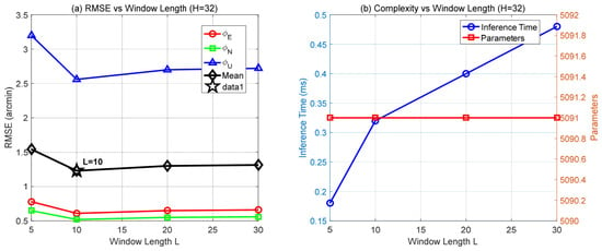
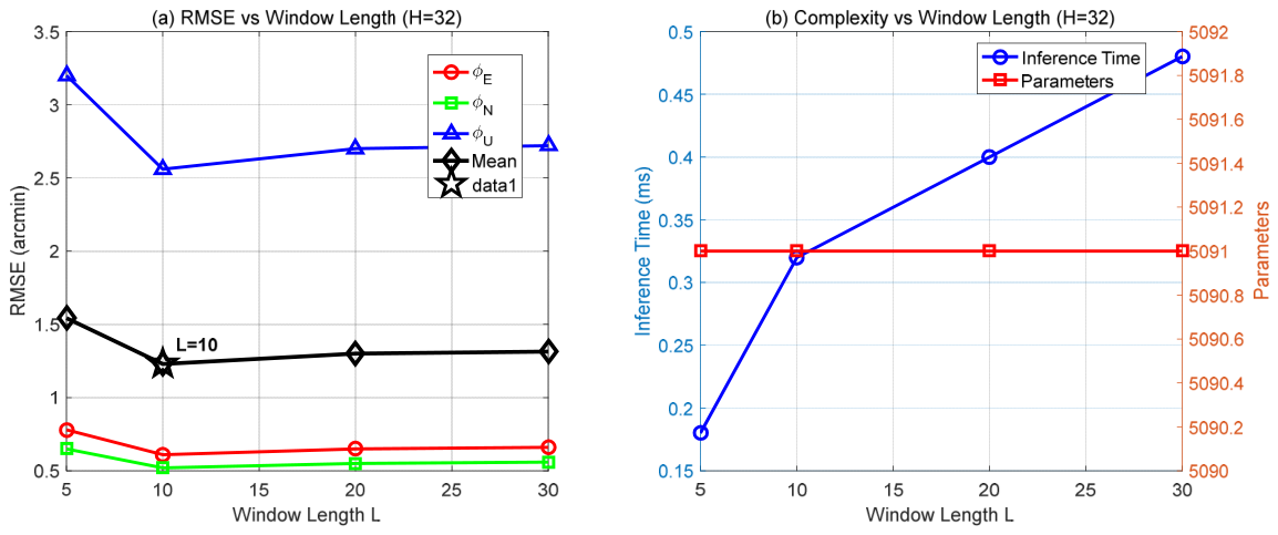
To determine a suitable LSTM architecture, the effects of input window length L and the number of hidden units H on misalignment angle estimation accuracy and computational complexity were investigated. The input window length determines the temporal span of historical observations available to the network, whereas the number of hidden units governs its capacity to capture the temporal characteristics of navigation errors. Prediction accuracy was evaluated using the root mean square error (RMSE) between the LSTM-predicted misalignment angles and their corresponding reference values on an independent validation subset, together with the mean RMSE across the three axes. Computational cost was characterized by the number of network parameters and the inference time per sample. First, the number of hidden units was fixed at H = 32, and the input window length was varied among 5, 10, 20, and 30. The results are presented in Figure 2.

Figure 2. Effects of input window length on LSTM estimation accuracy and computational complexity: (a) Variation in the RMSE of three-axis misalignment angle estimation with different input window lengths; (b) Variation in inference time and number of trainable parameters with different input window lengths.

When the window length increased from 5 to 10, the mean RMSE decreased from approximately 1.56 to 1.24 arcmin. Increasing the window length further to 20 or 30 did not consistently improve accuracy, while inference time continued to increase. Because changing the input window length does not alter the dimensions of the network weight matrices, the parameter count remained constant. These findings suggest that a short sequence may not capture sufficient historical information, whereas an excessively long input window incurs additional computational cost without further accuracy gains. Accordingly, L = 10 was selected as the input window length.

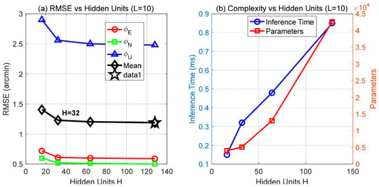
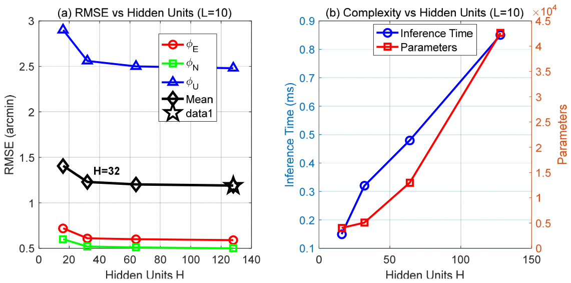
With the input window length fixed, the number of hidden units was varied among 16, 32, 64, and 128, as shown in Figure 3. Increasing the number of hidden units from 16 to 32 reduced the mean RMSE from approximately 1.41 to 1.23 arcmin, indicating improved misalignment angle estimation accuracy with increased network capacity. Further increasing the number of hidden units to 64 and 128, however, yielded only marginal improvements in RMSE, accompanied by substantial increases in model size and inference time. At H = 128, the inference time was approximately 0.85 ms per sample, compared with approximately 0.32 ms at H = 32. Thus, 32 hidden units provided relatively high accuracy at a considerably lower computational cost.

Figure 3. Effects of the number of hidden units on LSTM estimation accuracy and computational complexity: (a) Variation in the RMSE of three-axis misalignment angle estimation with different numbers of hidden units; (b) Variation in inference time and number of trainable parameters with different numbers of hidden units.

Based on these results, an input window of 10 steps and 32 hidden units were selected for the lightweight LSTM network. This configuration offers a reasonable balance among misalignment angle estimation accuracy, model size, and inference efficiency and serves as the basis for the subsequent evaluation of collaborative alignment performance.

4.1.3. LSTM Training and Convergence Analysis

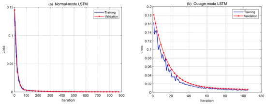
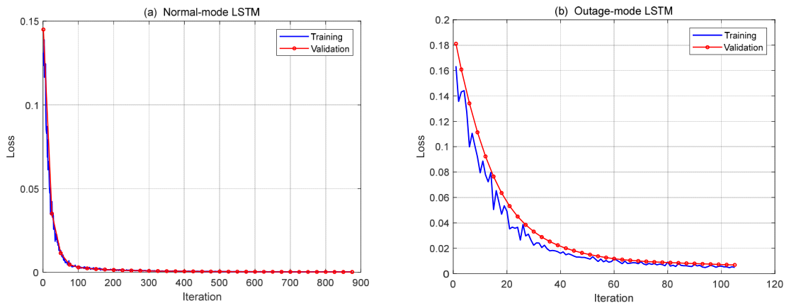
Separate LSTM networks were constructed for the GPS-available and GPS-outage modes. In the GPS-available mode, the LSTM used historical SINS/GPS position and velocity difference sequences to predict the three-axis misalignment angle estimation errors of the KF, providing auxiliary information for output-level correction. In the GPS-outage mode, the LSTM estimated the three-axis misalignment angles from inertial measurements and predicted navigation error states to generate auxiliary pseudo-measurements for the KF. The training and validation loss curves of the two networks are shown in Figure 4. Both networks employed mean squared error (MSE) as the loss function to quantify the discrepancy between the predicted and target values:

$$L_{\mathit{MSE}}={\displaystyle \frac{1}{3N}}{\displaystyle \sum _{i=1}^N{\displaystyle \sum _{j=1}^3{({\widehat{\mathrm{y}}}_{i,j}-{\mathrm{y}}_{i,j})}^2}}$$

(33)

where N is the number of samples, and ŷ_i,j and y_i,j denote the predicted and target values, respectively, for the j-th axis of the i-th sample. The training loss measures the fitting error on the training data, whereas the validation loss measures the prediction error on data not used for weight updates.

Figure 4. Training and validation loss curves of the LSTM networks under different GPS operating conditions: (a) GPS-available mode; (b) GPS-outage mode.

As shown in Figure 4a, both the training and validation losses of the GPS-available-mode LSTM decreased rapidly during the initial stage and gradually stabilized after approximately 150 iterations, with the two curves remaining close. By comparison, the GPS-outage-mode LSTM in Figure 4b converged more slowly: its training and validation losses decreased progressively and approached stable values after approximately 80 iterations. Neither network exhibited a sustained increase in validation loss or a pronounced separation between the training and validation curves, suggesting no clear evidence of overfitting on the current training and validation datasets.

4.2. Comparison of Alignment Performance Under Different GPS Conditions

To further evaluate the proposed KF–LSTM collaborative alignment method under different GPS operating conditions and compare it with conventional filtering and other learning-assisted methods, four reference methods were considered: conventional Kalman filtering (KF), adaptive Kalman filtering (AKF), multilayer perceptron-assisted Kalman filtering (KF–MLP), and gated recurrent unit-assisted Kalman filtering (KF–GRU). The conventional KF served as the baseline. The AKF adaptively adjusted the measurement noise covariance to improve its response to changes in observation noise, while KF–MLP and KF–GRU used feedforward and recurrent neural networks, respectively, to learn navigation error characteristics. These methods provide a basis for assessing the effects of different network structures on in-flight alignment accuracy.

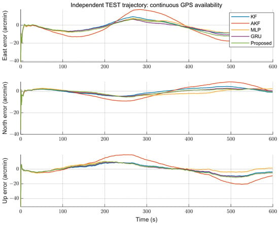
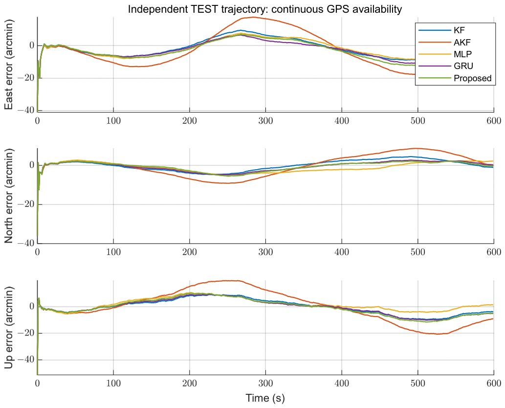
To ensure comparability, all methods were evaluated with identical initial conditions, motion trajectories, and sensor error parameters. The learning-assisted methods used the same dataset partitioning strategy, input information, and KF integration scheme. Under normal GPS conditions, each network predicted the three-axis misalignment angle estimation errors of the KF, and its predictions were incorporated through output-level correction. During GPS outages, each network generated misalignment-angle pseudo-measurements from inertial measurements and predicted navigation error states, which were then incorporated into the KF using the same measurement model. First, the three-axis misalignment angle estimation accuracy was compared under continuously available GPS measurements. The results are presented in Figure 5, and the corresponding RMSE statistics are given in Table 1.

Figure 5. Three-axis misalignment angle estimation errors of five methods under normal GPS conditions.

Table 1. RMSE comparison of five methods under normal GPS conditions (unit: arcmin).

Method	ɸE RMSE (′)	ɸN RMSE (′)	ɸU RMSE (′)	Mean RMSE (′)
KF	3.087	3.166	2.715	2.989
AKF	5.674	5.602	5.405	5.560
KF–MLP	3.072	3.008	2.712	2.950
KF–GRU	3.078	2.995	2.628	2.900
Proposed KF–LSTM	3.131	2.996	2.484	2.850

The east, north, and up RMSEs of the conventional KF were 3.087, 3.166, and 2.715 arcmin, respectively, yielding a mean RMSE of 2.989 arcmin. The mean RMSEs of KF–MLP, KF–GRU, and KF–LSTM were 2.950, 2.900, and 2.850 arcmin, corresponding to reductions of 1.30%, 2.98%, and 4.65%, respectively, relative to the conventional KF. By contrast, the mean RMSE of the AKF with the current parameter settings was 5.560 arcmin, showing no accuracy advantage. In terms of individual axes, KF–LSTM achieved some improvement in the north and up directions, whereas its east-direction error was slightly higher than that of the conventional KF. This suggests that the accuracy gains from output-level correction vary across axes.

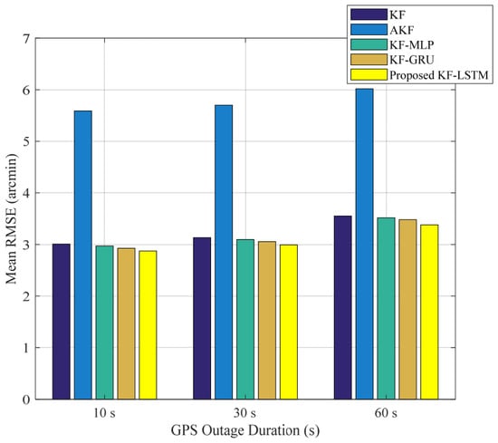
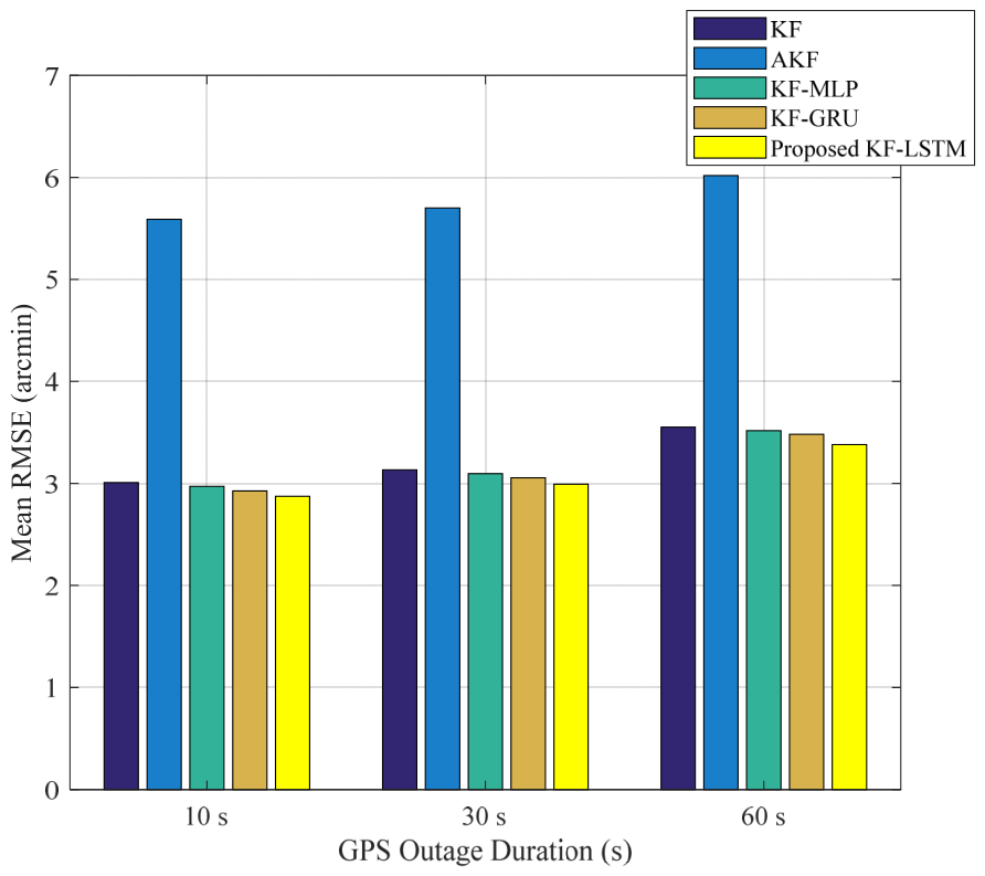
Next, complete GPS outages lasting 10, 30, and 60 s were introduced to investigate the effects of different observation interruption durations on estimation performance. During each outage, GPS position and velocity measurements were excluded. The conventional KF and AKF performed time updates based solely on the system state model, whereas the learning-assisted methods generated misalignment-angle pseudo-measurements to provide auxiliary KF updates. The mean RMSEs under the three outage conditions are compared in Figure 6.

Figure 6. Comparison of mean RMSEs among five alignment methods under different GPS outage durations.

As illustrated in Figure 6, the mean RMSE increased with GPS outage duration for all five methods. When the outage duration increased from 10 to 60 s, the mean RMSE of the conventional KF increased from 3.009 to 3.553 arcmin, whereas that of the proposed KF–LSTM method increased from 2.873 to 3.380 arcmin. For outage durations of 10, 30, and 60 s, the corresponding reductions in mean RMSE relative to the conventional KF were 4.51%, 4.491%, and 4.87%, respectively. These results indicate an improvement under the tested interruption scenarios. The detailed RMSE statistics are reported in Table 2.

Table 2. Comparison of misalignment angle RMSEs for different alignment methods under varying GPS outage durations (unit: arcmin).

GPS Outage	Method	E (′)	N (′)	U (′)	Mean (′)
10 s	KF	3.109	3.183	2.737	3.009
	AKF	5.702	5.629	5.437	5.589
	KF–MLP	3.165	3.017	2.730	2.971
	KF–GRU	3.115	3.008	2.655	2.926
	Proposed	3.113	2.995	2.511	2.873
30 s	KF	3.242	3.270	2.888	3.134
	AKF	5.806	5.720	5.574	5.700
	KF–MLP	3.310	3.101	2.878	3.096
	KF–GRU	3.262	3.093	2.814	3.056
	Proposed	3.253	3.060	2.666	2.993
60 s	KF	3.701	3.545	3.414	3.553
	AKF	6.115	5.949	5.987	6.017
	KF–MLP	3.766	3.377	3.407	3.517
	KF–GRU	3.718	3.368	3.356	3.481
	Proposed	3.658	3.308	3.173	3.380

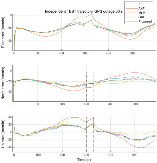
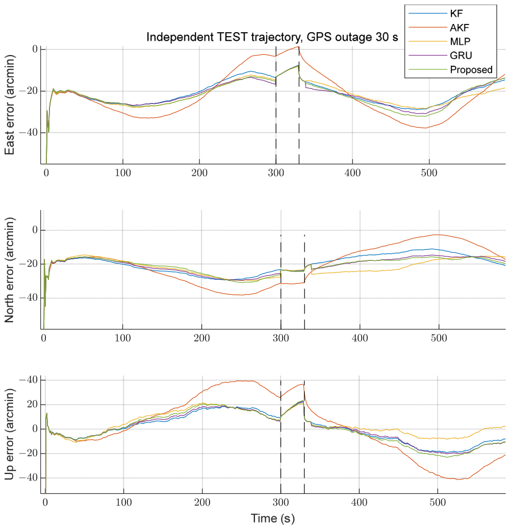
To further investigate the effect of changes in GPS measurement availability on in-flight alignment, a 30 s complete GPS outage was selected as a representative case. The three-axis misalignment angle estimation errors during outage and recovery are compared in Figure 7. GPS measurements were interrupted at 300 s and resumed at 330 s. During the outage, the conventional KF and AKF performed state prediction only, whereas the learning-assisted methods used network-generated misalignment-angle pseudo-measurements to provide auxiliary KF updates.

Figure 7. Three-axis misalignment angle estimation errors of different alignment methods during a 30 s GPS outage and subsequent recovery.

Before the GPS outage, the methods exhibited similar error trends, although their magnitudes differed. After GPS measurements became unavailable, their estimation errors changed to varying degrees. The AKF exhibited relatively large error deviations along some axes, whereas the KF–MLP, KF–GRU, and KF–LSTM estimates remained comparatively close. When GPS measurements resumed at 330 s, the methods again incorporated valid GPS observations for state correction, resulting in adjustments to the estimation errors and a subsequent tendency toward relatively stable behavior. In the proposed KF–LSTM method, misalignment-angle pseudo-measurements were used for auxiliary KF updates during the outage. Following GPS recovery, conventional measurement updates resumed, and output-level correction was reactivated after reconstruction of the required historical input sequence. The simulation results indicate that the method was able to switch between estimation strategies under different GPS operating conditions without sustained numerical divergence.

5. Vehicle Experiment

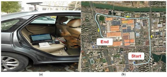
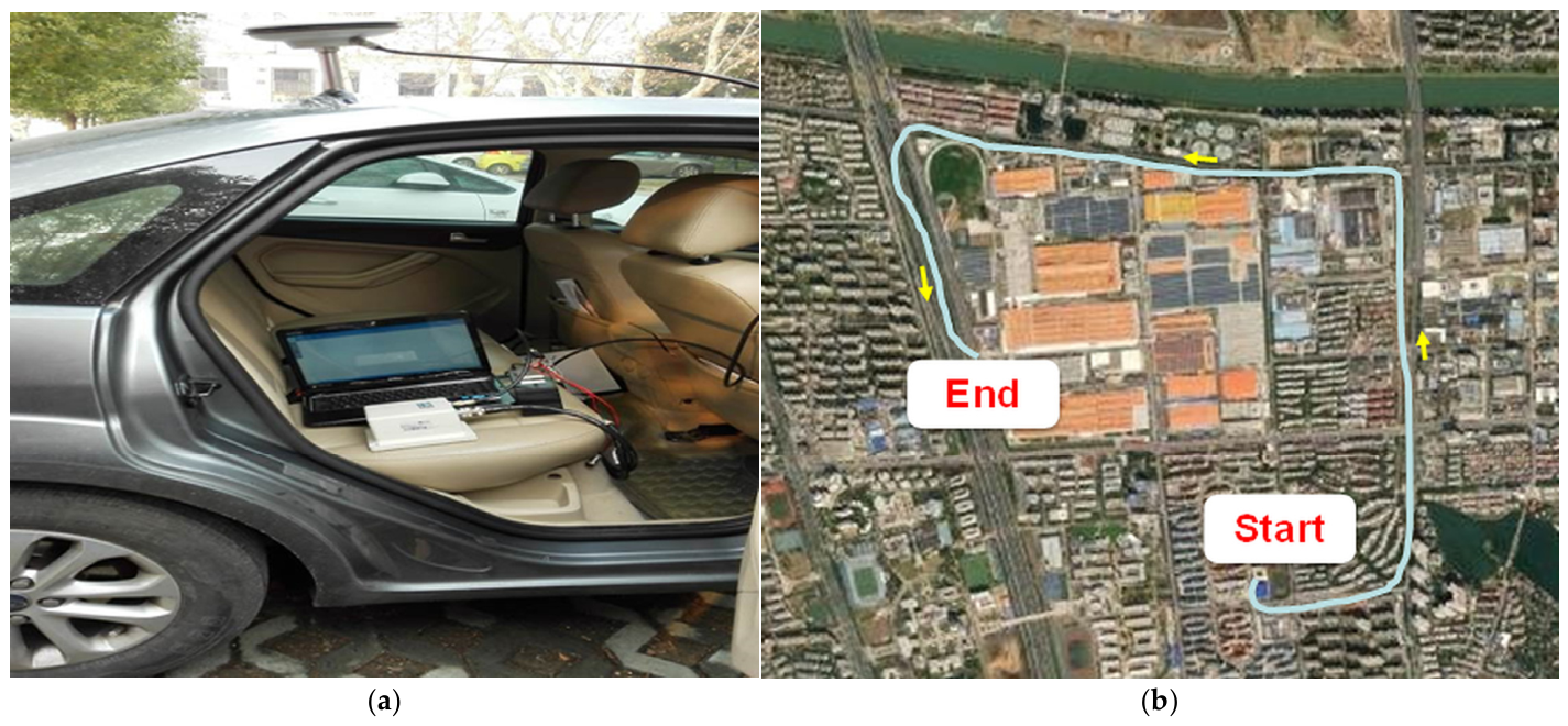
To further evaluate the applicability of the proposed KF–LSTM collaborative alignment method under practical motion conditions, a vehicle-based integrated navigation platform was established, as shown in Figure 8. The experimental system comprised a NovAtel SPAN-CPT reference navigation system and a STIM300 inertial measurement unit. The NovAtel SPAN-CPT provided the navigation reference, with specified roll and pitch accuracies of 0.008°, heading accuracy of 0.023°, velocity accuracy of 0.03 m/s, and position accuracy of 0.6 m. A Rauch–Tung–Striebel (RTS) smoother was applied to the reference navigation results to obtain post-processed attitude estimates for error evaluation.

Figure 8. Vehicle experiment platform and the corresponding field test trajectory. (a) NovAtel SPAN-CPT system used as the reference navigation system; (b) Trajectory of the field test conducted in Nanjing, China.

The vehicle experiment was conducted in Nanjing, China, with a data acquisition duration of 600 s. The inertial measurements and GPS position and velocity observations were used to construct a SINS/GPS integrated navigation system. The conventional KF and the proposed KF–LSTM method were then applied to the same dataset. Their three-axis attitude estimation errors and temporal behavior were compared to evaluate the proposed method under realistic sensor noise and vehicle motion conditions.

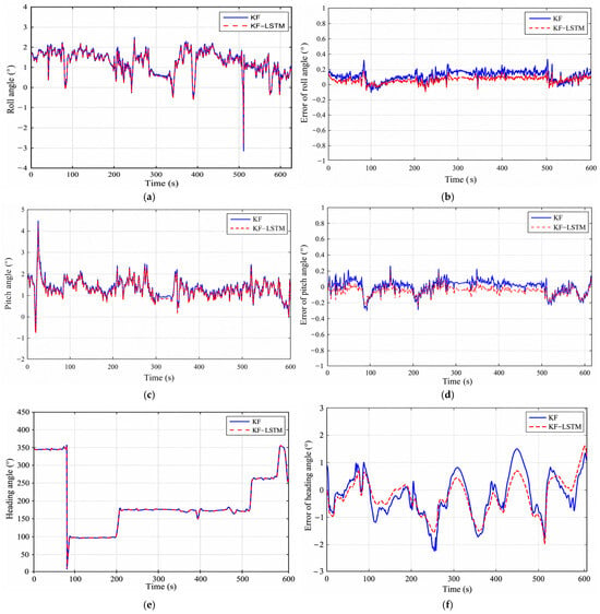
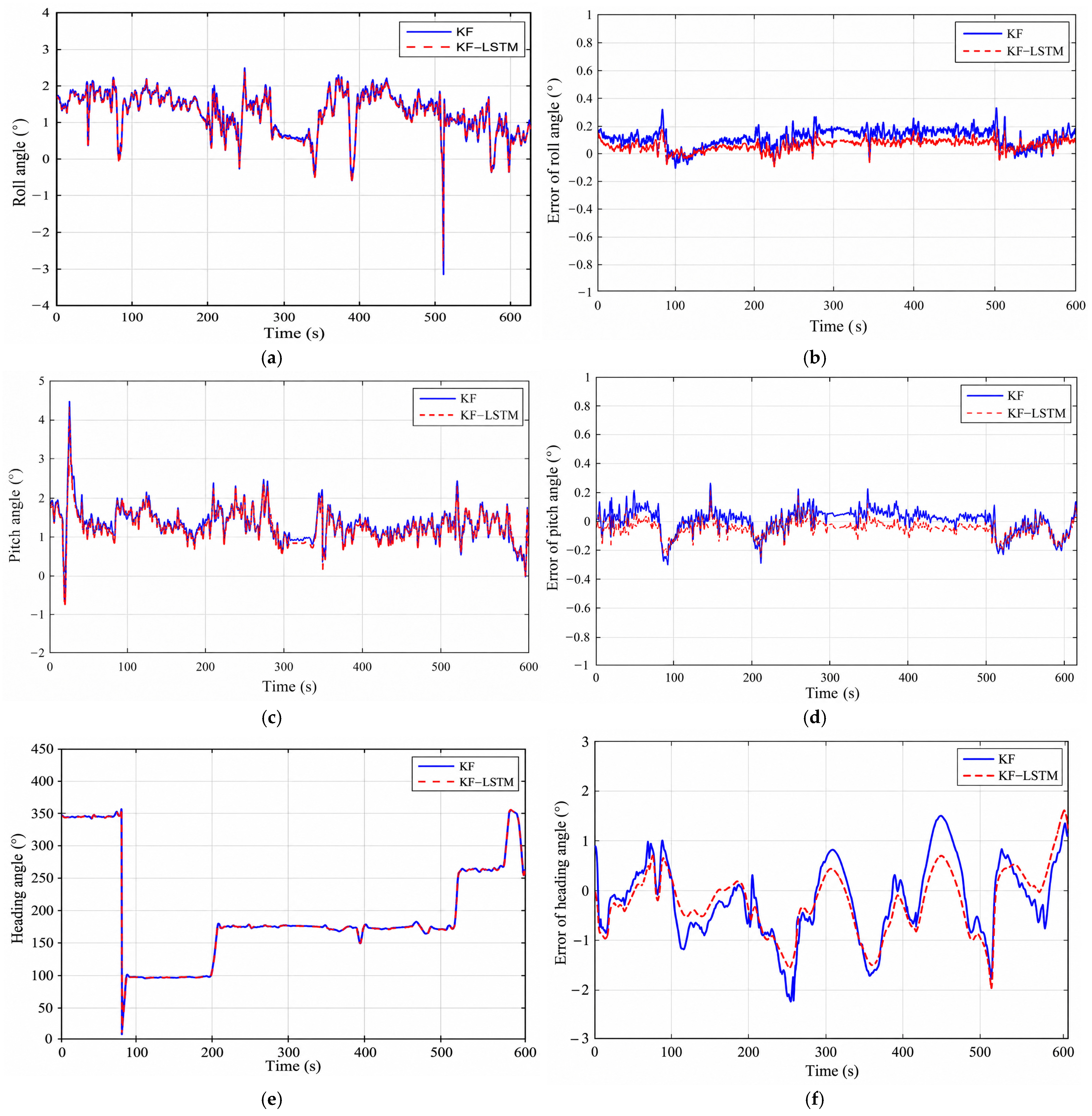
The three-axis attitude estimates obtained by the different methods and their errors relative to the reference system are presented in Figure 9. Roll, pitch, and heading RMSEs were used as the primary quantitative indicators, and the convergence behavior of the estimation errors was examined to assess estimation stability. The conventional KF was compared with KF–LSTM to evaluate the contribution of LSTM-based output-level correction to alignment performance under practical motion conditions. The corresponding statistical results, including the mean errors, standard deviations (SD), and root mean square errors (RMSE), are summarized in Table 3.

Figure 9. Comparison of three-axis attitude estimates and estimation errors between the conventional KF and the proposed KF–LSTM method in the vehicle experiment: (a) roll angle; (b) roll angle estimation error; (c) pitch angle; (d) pitch angle estimation error; (e) heading angle; (f) heading angle estimation error.

Table 3. Comparison of statistical errors (mean and standard deviation) for roll, pitch, and heading angles between the Kalman filter and the proposed KF–LSTM method in the vehicle experiment (unit: arcmin).

Errors	KF			KF–LSTM
	Mean (′)	SD (′)	RMSE (′)	Mean (′)	SD (′)	RMSE (′)
Roll	8.16	3.54	8.88	5.94	2.82	6.60
Pitch	3.42	5.22	6.24	0.48	3.84	3.84
Heading	−14.16	47.22	49.32	−17.82	38.64	42.54

In conclusion, compared with the traditional in-flight alignment algorithm based on the Kalman filter, the algorithm based on an LSTM neural network can improve the accuracy of the alignment. Especially when the system noise changes, the error angle estimation is obtained by using a large number of training samples to generate adaptive ability and construct the relationship between future and past information, so as to maintain a good in-flight alignment performance.

6. Conclusions

This paper proposed a lightweight KF–LSTM collaborative in-flight alignment method for SINS/GPS integrated navigation under varying GPS measurement conditions. The proposed method combines model-based state estimation with temporal feature learning through a GPS availability-dependent mode-switching strategy. Under normal GPS conditions, LSTM-based output-level correction is employed to refine the misalignment angle estimates without modifying the internal KF measurement update. During GPS outages, an independently trained LSTM generates misalignment-angle pseudo-measurements from inertial measurements and predicted navigation error states to support auxiliary KF updates. Following GPS recovery, conventional measurement updates are resumed, and output-level correction is reactivated after reconstruction of the required historical input sequence.

Simulation results showed that an LSTM configuration with a 10-step input window and 32 hidden units provided a reasonable balance between estimation accuracy and computational complexity. Comparisons with conventional KF, adaptive KF, KF–MLP, and KF–GRU under normal GPS conditions and different outage durations demonstrated the feasibility of the proposed collaborative strategy. The performance improvements varied across navigation axes and operating conditions, indicating that increased temporal modeling capability does not necessarily yield uniformly higher estimation accuracy. Vehicle experiments further indicated that LSTM-based output-level correction reduced the dispersion of attitude estimation errors, although improvements in estimation bias were not consistent across all attitude components.

Overall, the proposed method provides a mode-dependent framework for collaborative misalignment angle estimation under changing GPS measurement availability. Nevertheless, its performance during prolonged GPS outages and mode transitions remains dependent on the reliability of the learned pseudo-measurements. Future work will focus on improving pseudo-measurement uncertainty estimation, enhancing the stability of mode transitions, and validating the proposed approach using real flight data under representative GNSS-degraded and GNSS-denied conditions.

References

- Wu, Y.; Pan, X. Velocity/Position Integration Formula Part I: Application to In-Flight Coarse Alignment. IEEE Trans. Aerosp. Electron. Syst. 2013, 49, 1006–1023. [Google Scholar] [CrossRef] [Scilit]
- Lu, Z.; Li, J.; Zhang, X.; Feng, K.; Wei, X.; Zhang, D.; Mi, J.; Liu, Y. A New In-Flight Alignment Method with an Application to the Low-Cost SINS/GPS Integrated Navigation System. Sensors 2020, 20, 512. [Google Scholar] [CrossRef] [Scilit] [PubMed]
- Ning, X.; Huang, J.; Li, J. A Novel Robust Position Integration Optimization-Based Alignment Method for In-Flight Coarse Alignment. Sensors 2024, 24, 7000. [Google Scholar] [CrossRef] [Scilit] [PubMed]
- Mohamed, A.H.; Schwarz, K.P. Adaptive Kalman Filtering for INS/GPS. J. Geod. 1999, 73, 193–203. [Google Scholar] [CrossRef] [Scilit]
- Liu, Y.; Fan, X.; Lv, C.; Wu, J.; Li, L.; Ding, D. An Innovative Information Fusion Method with Adaptive Kalman Filter for Integrated INS/GPS Navigation of Autonomous Vehicles. Mech. Syst. Signal Process. 2018, 100, 605–616. [Google Scholar] [CrossRef] [Scilit]
- Sharaf, R.; Noureldin, A.; Osman, A.; El-Sheimy, N. Online INS/GPS Integration with a Radial Basis Function Neural Network. IEEE Aerosp. Electron. Syst. Mag. 2005, 20, 8–14. [Google Scholar] [CrossRef] [Scilit]
- Noureldin, A.; El-Shafie, A.; Bayoumi, M. GPS/INS Integration Utilizing Dynamic Neural Networks for Vehicular Navigation. Inf. Fusion 2011, 12, 48–57. [Google Scholar] [CrossRef] [Scilit]
- Dai, H.F.; Bian, H.W.; Wang, R.Y.; Ma, H. An INS/GNSS Integrated Navigation in GNSS Denied Environment Using Recurrent Neural Network. Def. Technol. 2020, 16, 334–340. [Google Scholar] [CrossRef] [Scilit]
- Sun, J.; Chen, Z.; Wang, F. A Novel ML-Aided Methodology for SINS/GPS Integrated Navigation Systems during GPS Outages. Remote Sens. 2022, 14, 5932. [Google Scholar] [CrossRef] [Scilit]
- Hochreiter, S.; Schmidhuber, J. Long Short-Term Memory. Neural Comput. 1997, 9, 1735–1780. [Google Scholar] [CrossRef] [Scilit] [PubMed]
- Fang, W.; Jiang, J.; Lu, S.; Gong, Y.; Tao, Y.; Tang, Y.; Yan, P.; Luo, H.; Liu, J. A LSTM Algorithm Estimating Pseudo Measurements for Aiding INS during GNSS Signal Outages. Remote Sens. 2020, 12, 256. [Google Scholar] [CrossRef] [Scilit]
- Cho, K.; van Merriënboer, B.; Gulcehre, C.; Bahdanau, D.; Bougares, F.; Schwenk, H.; Bengio, Y. Learning Phrase Representations Using RNN Encoder–Decoder for Statistical Machine Translation. In Proceedings of the 2014 Conference on Empirical Methods in Natural Language Processing (EMNLP), Doha, Qatar, 25–29 October 2014; pp. 1724–1734. [Google Scholar]
- Tang, Y.; Jiang, J.; Liu, J.; Yan, P.; Tao, Y.; Liu, J. A GRU and AKF-Based Hybrid Algorithm for Improving INS/GNSS Navigation Accuracy during GNSS Outage. Remote Sens. 2022, 14, 752. [Google Scholar] [CrossRef] [Scilit]
- Zhao, S.; Zhou, Y.; Huang, T. A Novel Method for AI-Assisted INS/GNSS Navigation System Based on CNN-GRU and CKF during GNSS Outage. Remote Sens. 2022, 14, 4494. [Google Scholar] [CrossRef] [Scilit]
- Alaeiyan, H.; Mosavi, M.R.; Ayatollahi, A. Improving the Performance of GPS/INS Integration during GPS Outage with Incremental Regularized LSTM Learning. Alex. Eng. J. 2024, 105, 137–155. [Google Scholar] [CrossRef] [Scilit]
- Wang, Y.; Wang, Q.; Zhang, H.; Duan, X. A Low-Cost GNSS/INS Integration Method Aided by Cascade-LSTM Pseudo-Velocity Measurement for Bridging GNSS Outages. Measurement 2025, 240, 115518, Corrigendum in Measurement 2025, 239, 115666. [Google Scholar] [CrossRef] [Scilit]
- Dai, W.; Han, H.; Wang, J.; Xiao, X.; Li, D.; Chen, C.; Wang, L. Enhanced CNN-BiLSTM-Attention Model for High-Precision Integrated Navigation During GNSS Outages. Remote Sens. 2025, 17, 1542. [Google Scholar] [CrossRef] [Scilit]
- Niu, S.; Li, J.; Hu, C.; Li, J.; Zhang, D.; Feng, K. A TCN-BiLSTM and ANR-IEKF Hybrid Framework for Sustained Vehicle Positioning During GNSS Outages. Sensors 2026, 26, 152. [Google Scholar] [CrossRef] [Scilit]
- Sahoo, A.K.; Klein, I. MoRPI-PINN: A Physics-Informed Framework for Mobile Robot Pure Inertial Navigation. Sci. Rep. 2026, 16, 19827. [Google Scholar] [CrossRef] [Scilit] [PubMed]
Disclaimer/Publisher’s Note: The statements, opinions and data contained in all publications are solely those of the individual author(s) and contributor(s) and not of MDPI and/or the editor(s). MDPI and/or the editor(s) disclaim responsibility for any injury to people or property resulting from any ideas, methods, instructions or products referred to in the content. |
© 2026 by the authors. Licensee MDPI, Basel, Switzerland. This article is an open access article distributed under the terms and conditions of the Creative Commons Attribution (CC BY) license.