Layer-Wise Evaluation of Hierarchical Distributed Control for Hybrid Alternating-Current and Direct-Current Microgrid Clusters Under Packet Loss and Forecast Uncertainty

Abstract

Hybrid alternating-current/direct-current (AC/DC) microgrid clusters require coordinated battery use, reliable restoration, and economic scheduling under communication and forecast disturbances. This study evaluates a three-layer distributed architecture in a constructed three-microgrid system using public load, solar, and price data from the California Independent System Operator (CAISO). The primary layer combines energy ratings and state of charge (SOC) for discharge sharing. The secondary layer models zero-order-hold (ZOH) receiver memory and tests mean-square stability under independent and identically distributed (IID) packet losses. The tertiary layer uses the alternating direction method of multipliers (ADMM) for distributed model predictive control (DMPC) with forecast correction and matched initial and terminal battery inventories across benchmark methods. On the selected stress day, compared with a grid-only baseline, operating cost and peak grid import decrease by 11.65% and 3.30%, respectively, while imported energy increases by 1.31%. The realized-cost difference from the centralized reference is 0.0029%. Supplementary tests examine longer discharge periods, complete communication outages, and reduced-order cross-layer behavior. Persistent-load-step tests reveal a restoration limitation of the original secondary controller. An integral candidate restores the tested deviations under combined disturbances. These findings characterize layer-specific performance and limited cross-layer responses within tested models. Field readiness and seasonal generalization remain unverified.

1. Introduction

Hybrid AC/DC microgrids connect photovoltaic (PV) generation, battery energy storage systems (BESSs), converter-interfaced resources, and mixed loads. Direct DC interfaces can reduce conversion stages, while AC feeders maintain compatibility with conventional equipment [1,2,3,4,5]. Interconnection allows microgrids to exchange power and operating flexibility [6]. Coordination then depends on electrical dynamics, available battery energy, forecast accuracy, and communication quality.

Hierarchical control separates fast local regulation, slower restoration, and economic scheduling [7,8,9,10]. Fixed power-sharing coefficients do not explicitly correct differences in battery SOC. Heterogeneous energy ratings make capacity-proportional sharing a useful reference: with equal discharge efficiencies, it gives equal SOC depletion rates. SOC adaptation can then be assessed against this neutral reference without attributing capacity-related depletion differences to the controller [11,12,13,14,15,16,17].

Distributed secondary controllers exchange neighboring states to compensate frequency and voltage deviations. Packet losses interrupt these updates and create stale information. Their effect depends on the receiver memory, loss duration, and temporal correlation. Communication-aware energy management and predictive voltage regulation have been studied under random drops, delays, and data loss [18,19,20,21,22]. These studies motivate stating the communication model and the scope of each stability claim explicitly.

Model predictive control (MPC) incorporates forecasts and operating limits within a receding-horizon optimization problem [23]. ADMM decomposes coupled schedules into local subproblems and coordination updates [24,25,26,27,28]. Recent work also examines how networked-microgrid ownership, control structure, and malicious coordination messages affect energy management [29,30]. Finite solver iterations and forecast correction must, therefore, be evaluated alongside the resulting physical constraints and realized costs.

Closely related studies address different parts of this problem. Li et al. [18] recover information lost in consensus-based energy management by exchanging accumulated power-mismatch estimates. Zhu et al. [25] combine MPC and block-wise ADMM to coordinate a honeycomb microgrid cluster. Liu and Starke [29] compare networked-microgrid energy management across ownership and control structures. The present study complements these approaches by evaluating capacity-aware discharge sharing, the explicit ZOH-memory stability model, and finite-iteration economic scheduling within one documented test configuration. It does not claim superiority over their controllers, because no common-model reproduction of those methods is performed.

The contribution is a reproducible layer-wise evaluation of an established hierarchical architecture. It makes three implementation choices explicit: capacity-aware SOC accounting, receiver memory in the secondary stability model, and joint primal–dual acceptance of energy-neutral DMPC schedules. The study provides an unsaturated-discharge contraction condition, an IID second-moment stability test, matched centralized benchmarks, and parameter and forecast diagnostics. Supplementary tests examine longer discharge intervals, complete communication outages, and a reduced-order cross-layer extension. They distinguish the original controller from an integral candidate and report unfavorable outcomes as well as successful cases. SOC adaptation, ZOH, ADMM, and MPC themselves are established methods [8,15,18,24,25]; their combination is not presented as a new general stability theorem.

2. System Description and Dynamic Modeling

2.1. Overall Configuration of the Hybrid AC/DC Microgrid Cluster

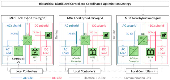
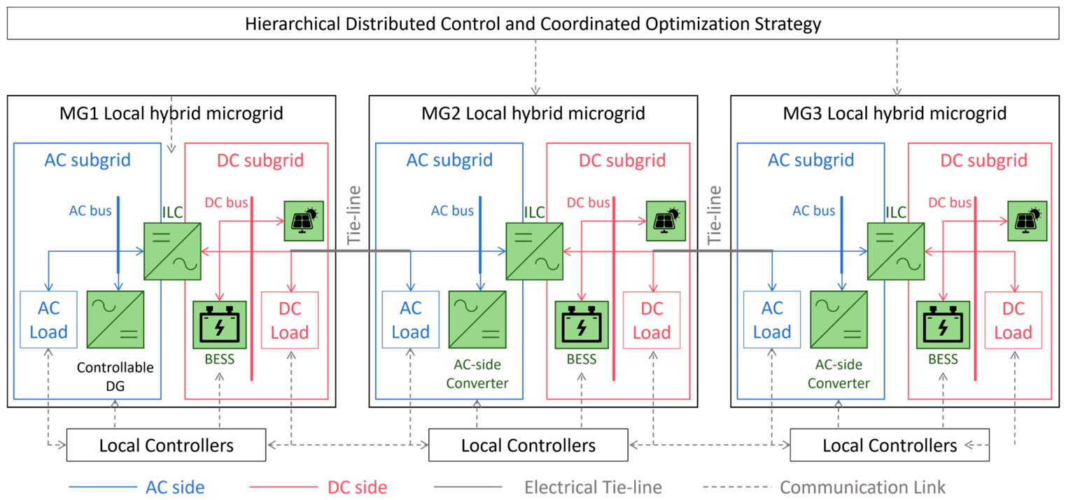
Figure 1 shows the three-microgrid test configuration. Each microgrid contains AC and DC subgrids, a bidirectional interlinking converter (ILC), PV generation, a BESS, local loads, and a grid-import interface. Electrical tie-lines allow power exchange, while a separate sparse communication graph carries coordination data. The schematic defines the architecture used to organize the layer-specific models. The controllable distributed generation (DG) shown in Figure 1 is schematic and is not included in the numerical benchmarks, which consider PV generation, BESS operation, grid imports, and tie-line exchanges.

Figure 1. Hybrid AC/DC microgrid cluster architecture. Electrical power exchange and information exchange serve distinct coordination functions.

The test system uses averaged, system-level representations. The scheduling model enforces energy and power constraints; the secondary experiment examines autonomous error restoration. They do not constitute a detailed electromagnetic model of the same electrical plant. Section 5.8 adds a reduced-order interface diagnostic. Switching transients, detailed ILC dynamics, and grid-connected/islanded PCC transitions remain outside the modeled scope.

2.2. AC-Side, DC-Side and Battery Models

For each AC subgrid, the inverter frequency is regulated by an active-power droop relation. With filtered power measurement, the primary frequency loop is represented as

$$f_i=f_0-m_{p,i}(P_i^m-P_i^{\ast }),$$

(1)

$${\tau }_p{\displaystyle \frac{d{P}_i^m}{dt}}=-P_i^m+P_i.$$

(2)

Here, $f_i$ and $f_0$ are the local and nominal frequencies; $P_i^m$ and $P_i^{\ast }$ are the measured and scheduled active powers. The droop coefficient is $m_{p,i}$, and the measurement-filter time constant is ${\tau }_p$. Around the operating point, active-power mismatch produces a frequency deviation [8,9,10].

The DC bus is modeled from capacitor energy balance as

$$C_{dc}{V}_{dc,i}{\displaystyle \frac{d{V}_{dc,i}}{dt}}=P_{ILC,i}+P_{PV,i}+P_{B,i}-P_{L,dc,i\cdot }.$$

(3)

Linearization around the nominal voltage $V_{dc,0}$ gives

$$C_{dc}{V}_{dc,0}{\displaystyle \frac{d\Delta V_{dc,i}}{dt}}=\Delta P_{ILC,i}+\Delta P_{PV,i}+\Delta P_{B,i}-\Delta P_{L,dc,i\cdot }.$$

(4)

Here, $C_{dc}$ is the DC-bus capacitance, $P_{ILC,i}$ is the ILC power transferred to the DC bus, and $P_{L,dc,i}$ is the DC-load power.

Equations (3) and (4) relate DC-voltage deviation to the mismatch among converter transfer, PV generation, BESS power, and demand. They identify the physical couplings that an integrated electrical model would need to represent [1,2,3,4,5].

The battery power response is described by the following first-order lag:

$${\tau }_B{\displaystyle \frac{d{P}_{B,i}}{dt}}=-P_{B,i}+P_{B,i}^{\ast }.$$

(5)

Here, ${\tau }_B$ is the battery-converter power-response time constant, and $P_{B,i}^{\ast }$ is the scheduled battery-power reference.

The SOC update follows the discrete energy balance:

$$s_i(k+1)=s_i(k)+{\displaystyle \frac{{\eta }_{\mathrm{c}}{P}_i^{\mathrm{ch}}(k)\Delta t_{\mathrm{s}}}{3600E_i}}-{\displaystyle \frac{P_i^{\mathrm{dis}}(k)\Delta t_{\mathrm{s}}}{3600{\eta }_{\mathrm{d}}{E}_i}}.$$

(6)

In Equation (6), $P_i^{\mathrm{ch}}$ and $P_i^{\mathrm{dis}}$ are in MW, $E_i$ is in MWh, and $\Delta t_{\mathrm{s}}$ is in seconds. The factor 1/3600 converts seconds to hours. Charging and discharging efficiencies are denoted by ${\eta }_{\mathrm{c}}$ and ${\eta }_d$, respectively [15,16,17].

2.3. Compact State-Space Representation and Constraints

The state-space notation collects AC-frequency deviation, DC-voltage deviation, BESS power, SOC, and restoration states:

$$x_i(k+1)=A_i{x}_i(k)+B_i{u}_i(k)+B_{w,i}{w}_i(k),$$

(7)

Here, $x_i$, $u_i$, and $w_i$ denote the local state, control-input, and exogenous-disturbance vectors, respectively. The matrices $A_i$, $B_i$, and $B_{w,i}$ are the local discrete-time state-transition, control-input, and disturbance-input matrices, respectively, with compatible dimensions. The scheduling constraints concern power and stored energy, while electricity prices enter the objective. The feasible set is represented by

$$\begin{array}{l}{P}_{g,i}^{\min }\le P_{g,i}\le P_{g,i}^{\max },\\ |P_{tie,ij}|\le P_{tie,ij}^{\max },\\ {\mathrm{SOC}}_i^{\min }\le {\mathrm{SOC}}_i\le {\mathrm{SOC}}_i^{\max }.\end{array}$$

(8)

For the linearized fast dynamics, small-signal stability requires the eigenvalues of the closed-loop matrix to remain in the stable region:

$$\begin{array}{l}\mathrm{Re}\left[\lambda (A_{cl})\right]<0 \mathrm{continuous} \mathrm{time},\\ \left|\lambda (A_{d,\mathrm{cl}})\right|<1 \mathrm{discrete} \mathrm{time}.\end{array}$$

(9)

Equation (9) concerns the autonomous linearized fast dynamics. It does not establish stability of the constrained, stochastic, multirate architecture. The implemented secondary model and its corresponding stability test are specified in Section 3.3 [8,9,10].

3. Hierarchical Distributed Control Design

3.1. Hierarchical Distributed Cooperative Control Framework

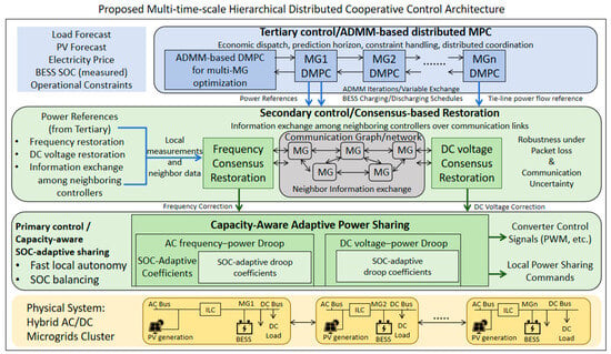
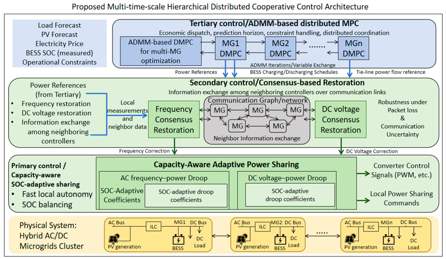
Figure 2 organizes local sharing, distributed restoration, and economic scheduling into three layers. The arrows identify reference and measurement interfaces. The main experiments evaluate the layers separately. Section 5.8 examines a supplementary reduced-order implementation of these interfaces and reports the differences from the main model. Computational performance is assessed through the measured centralized solution time and a separately defined distributed timing estimate.

Figure 2. Hierarchical distributed architecture and interlayer reference and measurement interfaces. The principal evaluation is layer-wise; the supplementary coupled model is specified separately.

In an implementation, the tertiary optimizer supplies battery and tie-line references, the primary layer executes feasible local power commands, and the secondary layer uses measured deviations and received neighbor states for restoration. Measured SOC must return to the next scheduling step. Separating update periods supports this organization, but separation alone is not a proof of closed-loop stability [7,8,9,14].

3.2. Primary Layer: SOC-Adaptive Power Sharing Gain Design

The fixed-sharing reference allocates aggregate discharge in proportion to rated battery energy. Let $s_i$ and $E_i$ denote the SOC and rated energy of BESS $i$; $P_{\Sigma }^{\mathrm{dis}}$ is the aggregate discharge request. The reference is

$$P_{i,\mathrm{fix}}^{\mathrm{dis}}=P_{\Sigma }^{\mathrm{dis}}{\displaystyle \frac{E_i}{{\displaystyle \sum _j{E}_j}}}.$$

(10)

For identical discharge efficiencies, equal $P_{i,\mathrm{fix}}^{\mathrm{dis}}/E_i$ gives equal SOC depletion rates and preserves the initial SOC difference. The adaptive multiplier is

$$\overline{s}={\displaystyle \frac{1}{N}}{\displaystyle \sum _i{s}_i},m_i=\mathrm{clip}\left[1+\kappa (s_i-\overline{s}),m_{\min },m_{\max }\right],$$

(11)

and the adaptive discharge allocation is

$$P_{i,\mathrm{adp}}^{\mathrm{dis}}=P_{\Sigma }^{\mathrm{dis}}{\displaystyle \frac{E_i{m}_i}{{\displaystyle \sum _j{E}_j}{m}_j}}.$$

(12)

A higher-SOC unit receives more discharge per unit of rated energy. Each allocation is bounded by the unit power limit. Any remaining request is redistributed over available discharge headroom; requests above aggregate feasible headroom must be rejected or reduced.

Without multiplier clipping, power saturation, or redistribution, $m_i(k)-m_j(k)=\kappa [s_i(k)-s_j(k)]$. Combining Equation (12) with the discharge part of Equation (6), and defining $d_{ij}\left(k\right)=s_i\left(k\right)-s_j\left(k\right)$, gives

$$d_{ij}(k+1)=\left[1-{\displaystyle \frac{P_{\Sigma }^{\mathrm{dis}}(k)\kappa \Delta t_{\mathrm{s}}}{3600{\eta }_{\mathrm{d}}{\displaystyle \sum _{\mathcal{l}}{E}_{\mathcal{l}}}{m}_{\mathcal{l}}(k)}}\right]d_{ij}(k),a(k)={\displaystyle \frac{P_{\Sigma }^{\mathrm{dis}}(k)\kappa \Delta t_{\mathrm{s}}}{3600{\eta }_{\mathrm{d}}{\displaystyle \sum _{\mathcal{l}}{E}_{\mathcal{l}}}{m}_{\mathcal{l}}(k)}}.$$

(13)

Pairwise disagreement contracts at sample $k$ when $\left|1-a\left(k\right)\right|<1$ or $0<a\left(k\right)<2$. The stronger condition, $0<a(k)\le 1$, gives monotonic contraction. Equation (13) assumes positive aggregate discharge, identical discharge efficiencies, and an unsaturated allocation throughout that sample. It does not prove convergence during charging, zero discharge, multiplier clipping, or power/SOC saturation. Section 5.2 includes a longer discharge test with these assumptions checked numerically.

3.3. Secondary Layer: Consensus Restoration Under Packet Loss

The secondary layer regulates a deviation state $x_i$; $x_i$ denotes either $\Delta f_i$ or $\Delta V_{dc,i}$. To match the numerical implementation, the consensus-restoration law includes compensation leakage and the received neighbor state:

$${\displaystyle \frac{d{u}_i^s}{dt}}=-c{\displaystyle {\sum }_{j\in N_i}{a}_{ij}\left(x_i-{\stackrel{\wedge }{x_j}}^{\left(i\right)}\right) }-k_r{x}_i-{\lambda }_u{u}_i^s.$$

(14)

In Equation (14), $c$ is the consensus gain, $k_r$ is the local restoration gain, $a_{ij}$ is the edge weight, and ${\mathcal{N}}_i$ is the neighbor set of node $i$. The added parameter ${\lambda }_u$ is the compensation leakage rate. The main secondary tests use ${\lambda }_u=1.6 s^{-1}$; the supplementary integral candidate sets it to zero. The hat denotes the ZOH-held value defined in Equation (15).

Let ${\gamma }_{ij}(k)\in \{0,1\}$ indicate delivery on the directed link from node $j$ to node $i$. The receiver keeps its last valid neighbor value when a packet is lost:

$${\widehat{x}}_j^{(i)}(k)={\gamma }_{ij}(k)x_j(k)+[1-{\gamma }_{ij}(k)]{\widehat{x}}_j^{(i)}(k-1).$$

(15)

At each communication sample, successful deliveries refresh the receiver memories first. The compensation state uses forward Euler on Equation (14); the deviation then uses the new compensation value:

$$u_i^s[k+1]=u_i^s[k]+\Delta t_s{\displaystyle \frac{d{u}_i^s}{dt}}[k].$$

(16)

$$x_i[k+1]=x_i[k]+\Delta t_s(-d_x{x}_i[k]+g_x{u}_i^s[k+1]).$$

(17)

Frequency and voltage use separate gains and receiver memories. The six directed links hold both variables. Together with the six deviation states and six compensation states, these twelve memory states form the 24-dimensional state $\xi (k)$. For delivery pattern $\sigma$, the autonomous sampled dynamics are

$$\xi (k+1)=A_{\sigma }\xi (k).$$

(18)

For link deliveries independent across links and samples, the second moment evolves under the probability-weighted Kronecker operator. Mean-square stability of this autonomous finite-dimensional linear model is equivalent to [31].

$$\rho \left({\displaystyle \sum _{\sigma }{\pi }_{\sigma }}{A}_{\sigma }\otimes A_{\sigma }\right)<1.$$

(19)

Here, ${\pi }_{\sigma }$ is the probability of delivery pattern $\sigma$. There are 64 patterns for six directed links. At loss rates 0, 0.1, 0.2, 0.3, and 0.4, the second-moment spectral radii are 0.874000, 0.874339, 0.874778, 0.875366, and 0.876193. Their values below unity establish mean-square stability for the specified autonomous IID model and gains. Correlated losses and forced responses require separate analysis; their simulated performance is discussed in Section 5.5 and Section 5.8.

3.4. Tertiary Layer: ADMM-Based DMPC with Prediction-Feedback Correction

Each microgrid solves a scheduling problem over horizon H. For microgrid $i$, the realized monetary cost is

$$J_{i,\mathrm{op}}={\displaystyle \sum _{k=0}^{H-1}\Delta }t\left[c_{i,k}^{\mathrm{e}}{P}_{i,k}^{\mathrm{g}}+c_1(P_{i,k}^{\mathrm{ch}}+P_{i,k}^{\mathrm{dis}})+c_2\left({(P_{i,k}^{\mathrm{ch}})}^2+{(P_{i,k}^{\mathrm{dis}})}^2\right)+c_{\mathrm{curt}}{P}_{i,k}^{\mathrm{curt}}\right].$$

(20)

The optimization objective additionally includes the stage-SOC regularizer:

$$J_{i,\mathrm{reg}}={\lambda }_s{\displaystyle \sum _{k=1}^H{(s_{i,k}-s^{\mathrm{ref}})}^2}.$$

(21)

The stage-SOC term shapes the trajectory and is excluded from reported monetary cost. A soft terminal-guidance term $J_{i,\mathrm{guide}}=15{[s_i(k+H)-0.55]}^2$ is used only when the prediction window ends before the daily endpoint. The cluster minimizes ${\displaystyle \sum _i(}{J}_{i,\mathrm{op}}+J_{i,\mathrm{reg}}+J_{i,\mathrm{guide}})$; at the daily endpoint, $J_{i,\mathrm{guide}}=0$. Local power balance, grid import, BESS operation, curtailment, SOC, and tie-line limits define the feasible set.

A common stored-energy inventory makes the economic comparison interpretable. Each optimized BESS starts from its specified initial SOC and returns to that value at the daily endpoint:

$$s_i(T)=s_i(0), i=1,\dots ,N.$$

(22)

When the prediction window reaches $T$, Equation (22) replaces soft terminal guidance. Energy neutrality means equal initial and final stored energy; it does not mean lossless storage. With nonzero cycling and efficiencies below unity, grid energy may increase even when time-varying prices allow monetary savings.

Define $J_i(u_i)=J_{i,\mathrm{op}}+J_{i,\mathrm{reg}}+J_{i,\mathrm{guide}}$ as the local optimization objective. The realized monetary costs are evaluated using Equation (20) on the executed schedules and exclude the SOC regularization, terminal-guidance, and ADMM penalty terms. ADMM decomposes the tie-line consistency constraints. For each oriented tie line (a, b), the local flow vectors $p_{ab}$ and $p_{ba}$ are positive for export from their respective nodes. In the local update below, $z_i$ collects the signed consensus copies $+z_{ab}$ at node a and $-z_{ab}$ at node b, while $y_i$ collects the corresponding scaled dual variables.

$$u_i^{l+1}=\arg {\min }_{u_i\in U_i}\left[J_i(u_i)+{\displaystyle \frac{\rho }{2}}{‖P_{tie,i}(u_i)-z_i^l+y_i^l‖}_2^2\right],$$

(23)

$$\begin{array}{l}{z}_{ab}^{l+1}={\displaystyle \frac{1}{2}}\left[\left(p_{ab}^{l+1}+y_{ab}^l\right)-\left(p_{ba}^{l+1}+y_{ba}^l\right)\right],\\ y_{ab}^{l+1}=y_{ab}^l+p_{ab}^{l+1}-z_{ab}^{l+1},\\ y_{ba}^{l+1}=y_{ba}^l+p_{ba}^{l+1}+z_{ab}^{l+1}.\end{array}$$

(24)

Here, $y_{ab}$ and $y_{ba}$ are the corresponding components of the local scaled dual vectors.

The grid-only, centralized-MPC, and DMPC benchmarks are defined in Section 5.1. Their common model inputs and metric calculations are used for all benchmark comparisons.

All three strategies use initial SOC [0.62, 0.60, 0.58]. The grid-only baseline leaves batteries idle and, therefore, satisfies the daily terminal condition. Centralized MPC and DMPC impose $s_i\left(T\right)=s_i\left(0\right)$ for each BESS.

Under the adopted linear constraints and quadratic penalties, the local scheduling problems are convex quadratic programs [23,24,25]. This model-level convexity does not turn a finite residual threshold or a realized-cost comparison into a certified optimality bound. ADMM coordination uses the residuals [24,26,27,28]:

$$r_{\mathrm{p}}^{\mathcal{l}}={\left[{\displaystyle \sum _{(a,b)}\left(\Vert p_{ab}^{\mathcal{l}}-z_{ab}^{\mathcal{l}}{\Vert }_2^2+\Vert p_{ba}^{\mathcal{l}}+z_{ab}^{\mathcal{l}}{\Vert }_2^2\right)}\right]}^{1/2},r_{\mathrm{d}}^{\mathcal{l}}=\rho {\left[2{\displaystyle \sum _{(a,b)}\Vert z_{ab}^{\mathcal{l}}-z_{ab}^{\mathcal{l}-1}{\Vert }_2^2}\right]}^{1/2}.$$

(25)

At iteration $\mathcal{l}$, the primal residual measures tie-line consensus mismatch; the dual residual measures the change in the consensus schedule scaled by $\rho$. Both norms must be, at most, 10⁻³ before the first control action is accepted. The limit is 500 iterations. The main controller enables adaptive residual balancing, starting from $\rho =5$, checking every 10 iterations with $\mu =10$, scaling by 2, and keeping $\rho$ in [0.1, 20]. When the primal norm exceeds ten times the dual norm, the penalty is doubled; when the dual norm exceeds ten times the primal norm, it is halved, subject to the bounds. Scaled dual variables are multiplied by the old penalty divided by the new penalty. The diagnostic absolute and relative tolerances are 10⁻⁴ and 10⁻³; execution uses a fixed common 10⁻³ gate. A failed solve is recorded as a failed step; its control action is not executed. All main stress-day steps passed; this study does not evaluate a deployment fallback for rejected steps.

Forecast mismatch is mitigated by prediction-feedback correction. The corrected net-demand forecast is updated as

$${\widehat{N}}_i^{corr}(t+k|t)={\widehat{N}}_i^{DA}(t+k|t)+{\alpha }^k{\epsilon }_i(t),{\epsilon }_i(t)=N_i^{real}(t)-{\widehat{N}}_i^{DA}(t).$$

(26)

The feedback coefficient is selected using up to 30 available dates preceding 16 October 2025; seven dates are available in the present dataset. Candidate coefficients minimize combined load and solar squared prediction error. The selected value $\alpha =0.8$ is fixed before the stress-day evaluation. The original fitting routine uses sample offsets over concatenated records. A supplementary check restricting one- to six-hour prediction pairs to the same date also selects 0.8, so the reported coefficient is unchanged. Reuse for all eight retrospective dates is a different protocol, described in Section 5.6.

4. Python Implementation and Dataset Construction

4.1. Python-Based Experimental Framework and Test Cases

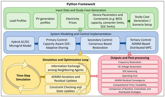
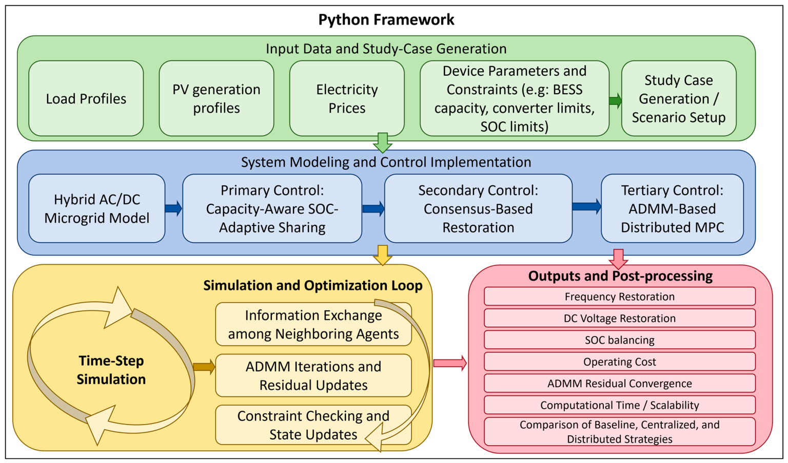
An author-developed Python framework performs data acquisition, preprocessing, model simulation, optimization, and reporting. Figure 3 shows the workflow. CAISO records are converted to the America/Los Angeles time zone, aligned hourly, and scaled by fixed factors. The same factor is applied to each actual/forecast pair before mapping it to a test microgrid [32].

Figure 3. Data preparation, layer-wise simulation, and validation workflow. Exported trajectories, configuration files, and solver diagnostics link inputs to the reported results.

The workflow exports trajectories, corrected forecasts, schedules, monetary cost components, residuals, constraint checks, Monte Carlo summaries, and timing diagnostics. A reproducibility manifest records software versions, random seeds, configuration values, and SHA-256 hashes. The accompanying numerical evidence package separates the principal benchmarks from the supplementary experiments.

The CAISO OASIS queries are SLD FCST for load, SLD REN FCST for solar, and PRC LMP for day-ahead prices [32]. Load zones PGE-TAC, SCE-TAC, and SDGE-TAC; solar hubs NP15, ZP26, and SP15; and price nodes DLAP PGAE-APND, DLAP SCE-APND, and DLAP SDGE-APND are mapped to MG1–MG3. The load and solar profiles are scaled to their specified peak ratings using the maximum actual values over the available data. The same scaling factors are applied to the corresponding forecasts, while day-ahead prices retain their original USD/MWh values. This produces a test system, not three identified CAISO microgrids. A deliberately weighted stress score selects 16 October 2025 from eight dates. The min–max-normalized indicators of price volatility, maximum net-load ramp, and forecast mean absolute error (MAE) have weights 0.40, 0.35, and 0.25. The selected score is 0.889991. This deterministic selection emphasizes stress and does not represent random sampling.

The principal numerical experiments use Python 3.9.7, NumPy 2.0.2, pandas 2.3.3, CVXPY 1.7.5, and OSQP 1.1.1. The numerical plots were generated using Matplotlib 3.9.4. The diagrams were prepared in Microsoft PowerPoint. Optimization uses OSQP through CVXPY with warm starts and the recorded library defaults. Timing tests use a Windows AMD64 workstation with 16 logical CPU cores. Seeds 7, 20260819, and 17 specify the representative secondary trajectory, packet-loss Monte Carlo study, and scalability test, respectively. Supplementary duration and deterministic-outage calculations use Python 3.12.14, NumPy 2.3.5, and pandas 3.0.1.

Table 1 lists the system ratings and controller and optimizer settings used in the principal experiments. Their selection basis is explained in Section 4.2. The configuration file records the adopted values; it is an implementation source, not evidence of physical parameter identification.

Table 1. System ratings and controller and optimizer settings for the principal layer-wise experiments.

Category	Parameter	Value
System	Nodes/references/power limits	3 MGs; 50 Hz; 400 V; import ≤ 3.0 MW per MG; tie power ± 0.7 MW
Profiles	Target load/PV peaks (MG1–MG3)	1.8/1.5/1.2 MW; 1.3/1.1/0.9 MW
BESS	Energy/power (MG1–MG3)	2.4/2.0/1.6 MWh; 1.0/0.9/0.8 MW
Scheduling	Initial SOC/limits/daily target	0.62/0.60/0.58; [0.15, 0.90] p.u.; each final SOC equals its own initial SOC
Primary test	Energy/initial SOC/request	2.4/2.0 MWh; 0.80/0.60 p.u.; 0.6 MW
Primary test	Duration/integration/efficiency	10 min; 1 s; discharge efficiency 0.95
Primary control	Gain/multiplier limits	3.0; [0.2, 1.8]
Secondary	Graph/duration/sample	Three-node bidirectional ring; 40 s; 0.05 s
Secondary	Initial frequency/DC errors	[−0.28, −0.20, −0.12] Hz; [−10, −7, −4] V
Secondary	Frequency c/kr/gx/dx	1.2/0.7/1.0/1.0 s−1
Secondary	DC voltage c/kr/gx/dx	1.5/0.85/0.9/1.1 s−1
Secondary	Leakage/reporting bands	1.6 s−1; 0.01 Hz and 0.5 V
Packet loss	Rates/models/runs/burst length	0–40%; IID and Gilbert–Elliott; 200 per condition; mean bad state 5 samples (0.25 s)
Tertiary	Step/horizon/efficiencies	1 h; 24 h; charge/discharge 0.95/0.95
Cost	Battery linear/quadratic/curtailment	1.8 USD/MWh; 3.5 USD/(MW2 h); 8.0 USD/MWh
SOC terms	Reference/stage/soft terminal weights	0.55 p.u.; 5.0; 15.0 (soft guidance before daily endpoint only)
ADMM	Initial rho/range/budget	5.0; [0.1, 20]; maximum 500 iterations
ADMM	Execution gate/diagnostic tolerances	Both norms ≤ 10−3; absolute 10−4, relative 10−3
ADMM	Adaptive balancing	Enabled; every 10 iterations; ratio 10; scale 2; rescale dual variables
Forecast	Calibration/coefficient	Up to 30 prior available dates (7 used); $\alpha =0.8$
Scalability	Nodes/horizon/assumed communication	2–10; 12 h; up to 500 iterations; 1.2 ms per iteration

4.2. Parameter Selection and Reproducibility

The system values in Table 1 are author-defined benchmark settings. They are not manufacturer specifications or estimates inferred from CAISO profiles. Peak load ratings of 1.8/1.5/1.2 MW and PV ratings of 1.3/1.1/0.9 MW set the profile scales. Battery ratings introduce heterogeneous storage with energy-to-power ratios of 2.4, 2.22, and 2.0 h. The 3.0 MW per-node import bound and 0.7 MW tie bound define the feasible exchange envelope. Nominal 50 Hz and 400 V are reference values for the control model; the CAISO data supply load, solar, and price shapes rather than these electrical ratings.

Initial scheduling SOCs 0.62/0.60/0.58 provide a small inventory difference, while the primary mechanism test deliberately uses 0.80/0.60. SOC limits 0.15–0.90 and charge/discharge efficiencies 0.95 are illustrative storage assumptions. They reserve energy margins and model conversion losses without identifying a particular battery technology. The adaptive gain 3 and multiplier bounds 0.2–1.8 define the tested sharing sensitivity and retain positive weights. The 0.6 MW test request remains below aggregate battery power capability.

The three-node bidirectional ring defines six independent directed message channels. The 0.05 s communication step, 40 s restoration window, initial deviations, and secondary gains specify a reduced-order numerical experiment; they are not tuned converter gains from a physical installation. Frequency uses consensus/restoration/state/damping gains 1.2/0.7/1.0/1.0 s⁻¹; DC voltage uses 1.5/0.85/0.9/1.1 s⁻¹. Compensation leakage is 1.6 s⁻¹. The 0.01 Hz and 0.5 V bands are reporting criteria, not a grid-code compliance test. IID stability and Monte Carlo tests check the adopted settings within their respective assumptions.

Hourly scheduling and a 24 h horizon cover one daily energy cycle. Grid-energy prices come from CAISO; battery linear/quadratic coefficients 1.8 USD/MWh and 3.5 USD/(MW² h), curtailment coefficient 8 USD/MWh, and SOC weights 5 and 15 are benchmark modeling weights. They are not measured degradation costs or regulated tariffs. ADMM settings define a reproducible numerical acceptance policy. Fixed-penalty and 6/12/24 h sensitivity tests examine that policy without identifying a universally optimal tuning. The supplementary experiment configurations and full parameter registry are included with the numerical evidence.

4.3. Supplementary Experimental Protocols

The duration test extends the original two-battery discharge calculation to 30, 60, and 120 min without changing ratings, request, efficiency, gain, or sample period. The complete-outage test uses the original 24-state secondary update initialized with Table 1 deviations and the initial neighbor measurements. All six links stop delivering at t = 0.5 s for 1, 5, 10, 20, 40, or 60 s, and then resume perfect delivery. Simulation lasts 80 s. Data age is measured immediately before the receiver update; its maximum is outage duration plus one 0.05 s sample. These deterministic scenarios isolate stale ZOH memory and are not an additional Bernoulli loss-rate sweep.

The coupled diagnostic initializes the 17:00 operating point on 16 October from the tertiary–primary execution bridge and re-solves the event-hour ADMM schedule. BESS and tie-line references feed reduced-order actuators. The integration, primary-execution, and communication steps are 0.005 s, 1 s, and 0.05 s, respectively, over a 40 s event. A persistent 0.4 MW load step is applied to MG1 at 0.5 s. The original secondary leakage of 1.6 s⁻¹ is compared with an integral candidate with zero leakage; other event parameters are held fixed. The dynamic controller scales the secondary update by 0.18 and differs from the stand-alone error model. This explicit variant comparison is not a validation of Equation (19) for the coupled plant.

Joint tests use the integral candidate and preserve the hourly actual-minus-forecast residual sequence at multipliers 1, 1.5, and 2. Solar forecasts are clipped at zero and corrected using coefficient 0.8. The event plant receives the residual relative to the corrected forecast. Five channel conditions (no loss, 20%/40% IID, and 20%/40% burst) and two additional-step values (0/0.4 MW) give 30 cells. Each cell has 50 communication seeds; six non-deterministic cells ranked by non-settling, frequency peak, and voltage peak receive 200 extra seeds, giving 2700 events. Random repetition quantifies communication variation, not independent forecast trajectories. Event SOC is transferred to the next hourly solve by adding its actual-minus-nominal 40 s energy difference to the nominal hour-end SOC. This handoff is an approximation. Subsequent costs cover only 18:00–24:00 and exclude incremental event-load expenditure.

5. Results and Discussion

The principal results address local SOC sharing, secondary restoration, forecast correction, economic dispatch, and optimizer acceptance. Supplementary tests in Section 5.8 examine complete outages and a reduced-order coupled interface. Each result is interpreted for its own model and protocol.

5.1. Benchmark Strategies and Metrics

The grid-only baseline disables battery cycling and tie-line exchange. Centralized MPC and DMPC begin at [0.62, 0.60, 0.58] and impose $s_i\left(T\right)=s_i\left(0\right)$. Both optimizers use the same load/PV forecasts, feedback correction, prices, device ratings, efficiencies, horizon, regularization, and operating constraints. They differ in how the coupled scheduling problem is solved. The baseline is a reference for the economic value of scheduling resources, not a controller with the same enabled actuators.

For the economic comparison, every strategy uses the same 24 hourly realizations. Grid-only supplies local net demand subject to its import bound and curtails surplus PV; it leaves batteries and ties idle. The two optimizers solve 24 shrinking daily horizons, apply only the first accepted action, and update SOC from the realized schedule. Realized grid import is reconstructed with actual load/PV, executed battery power, and the accepted tie schedule. Daily import is the sum of node imports times 1 h; peak import is the maximum hourly cluster sum; throughput integrates charge plus discharge. Daily monetary cost sums grid-energy, linear and quadratic battery, and curtailment terms in Equation (20). The centralized discrepancy divides the absolute difference in realized costs by centralized cost. SOC regularization remains a separate optimization diagnostic. The common daily terminal equality prevents stored-energy depletion from being counted as economic savings. Reported differences and percentages are calculated from unrounded outputs.

Metrics distinguish energy, instantaneous power, monetary cost, and numerical diagnostics. SOC disagreement is the pairwise difference in the two-battery test. Settling uses the maximum node error and the stated reporting bands. Daily import and throughput integrate hourly power; peak import is the largest hourly cluster sum. Monetary cost follows Equation (20), excluding SOC regularization. ADMM residuals, tie mismatch, terminal deviation, and physical-constraint violations are reported separately.

5.2. SOC Balancing and Restoration Performance

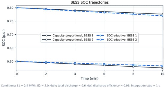
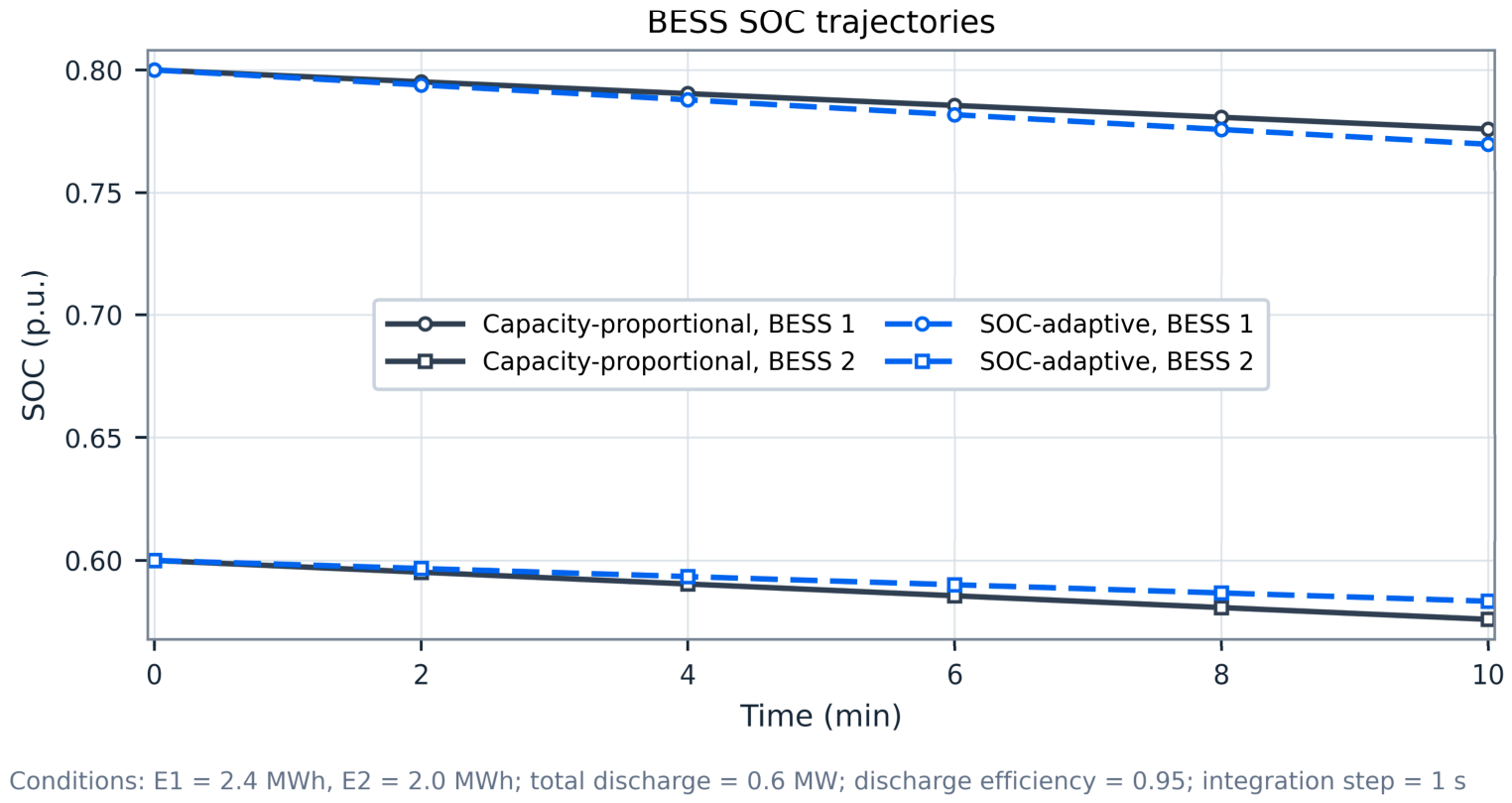
Figure 4 compares the same 0.6 MW discharge request across two BESSs of 2.4 and 2.0 MWh. Initial SOCs are 0.80 and 0.60, discharge efficiency is 0.95, and integration uses 1 s steps. After 10 min, fixed capacity-proportional sharing retains a 0.2000 p.u. gap; SOC-adaptive sharing gives 0.1865 p.u., a 6.75% reduction. Keeping the same settings and extending discharge to 30, 60, and 120 min gives gaps of 0.1621, 0.1312, and 0.08585 p.u. (reductions of 18.95%, 34.38%, and 57.08%). The extended trajectories do not activate weight clipping or power/SOC limits; minimum SOC is 0.3752 p.u. The short-run improvement reflects the slow energy time scale. These discharge tests do not establish balancing under charging or active constraints.

Figure 4. Two-battery SOC trajectories under capacity-proportional and SOC-adaptive sharing over 10 min. Longer-duration results use the same discharge request and ratings.

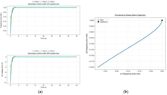
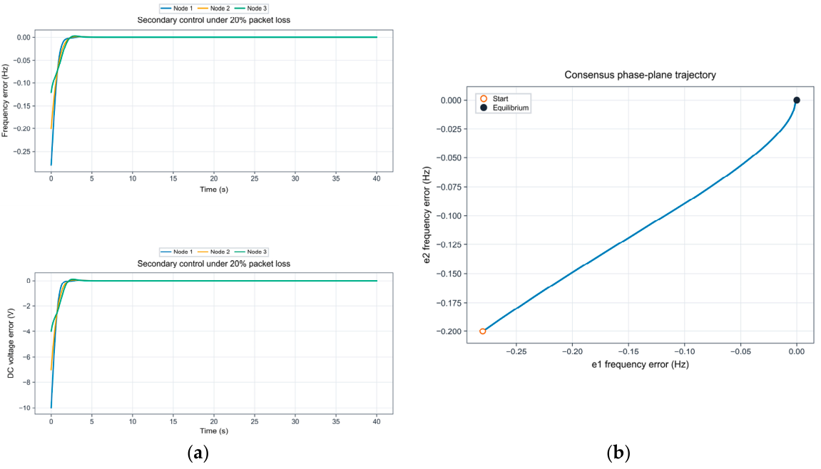
Figure 5a shows frequency- and DC-voltage-error recovery for one 20% IID packet-loss realization (seed 7). Figure 5b shows the frequency-error consensus phase plane without packet loss. Both autonomous tests use the initial deviations in Table 1. Statistical results appear in Section 5.5; persistent forcing is examined separately in Section 5.8 [18,19,20,21,22].

Figure 5. Secondary-controller responses: (a) frequency- and DC-voltage-error recovery under 20% IID packet loss (seed 7); (b) frequency-error consensus phase plane without packet loss. In panel (b), the blue curve plots the frequency error at Node 2 against that at Node 1.

5.3. Forecast Correction, Dispatch, and Economic Performance

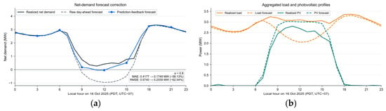
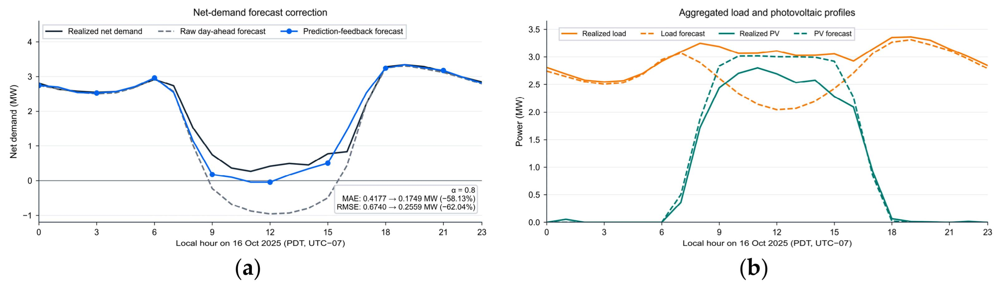
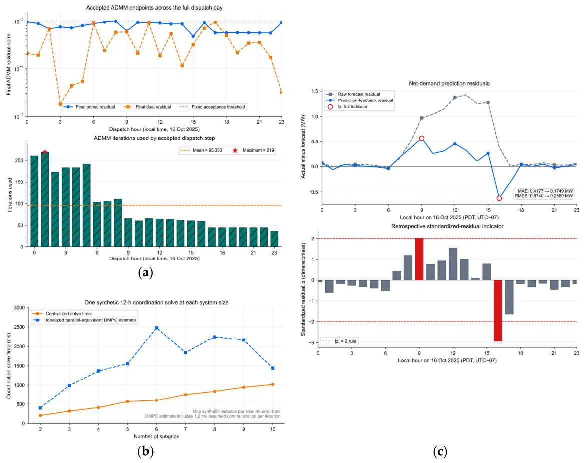
On 16 October 2025, prediction feedback reduces net-demand MAE from 0.4177 to 0.1749 MW and root-mean-square error (RMSE) from 0.6740 to 0.2559 MW, decreases of 58.13% and 62.04%. Figure 6 compares the resulting hourly profiles. The coefficient 0.8 is fixed using the pre-target calibration described in Section 3.4. These metrics describe the deliberately selected day.

Figure 6. Prediction-feedback diagnostics on 16 October 2025: (a) realized net demand, raw day-ahead forecast, and corrected forecast; (b) aggregated realized and forecast load and photovoltaic profiles.

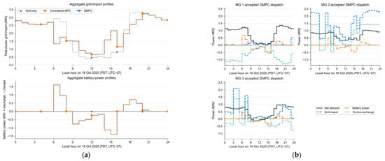
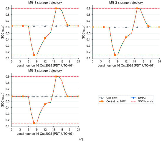
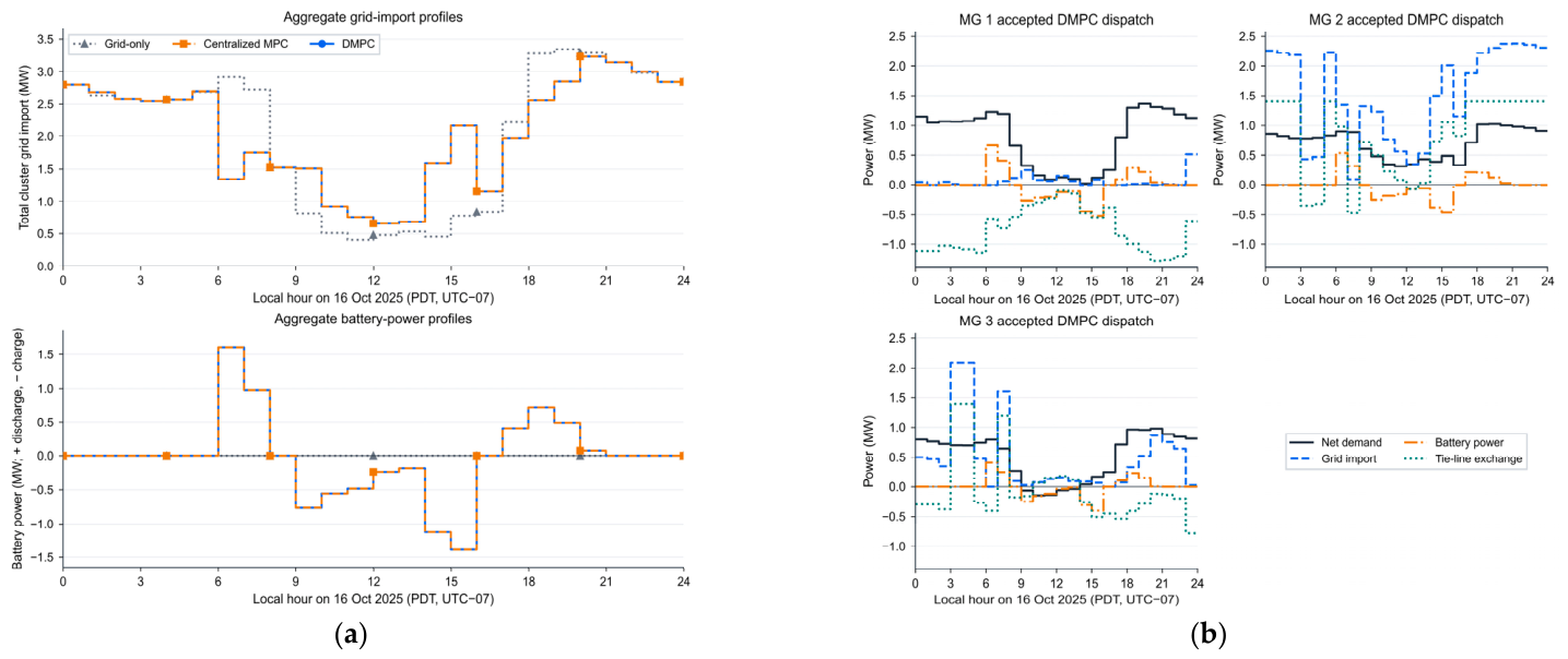
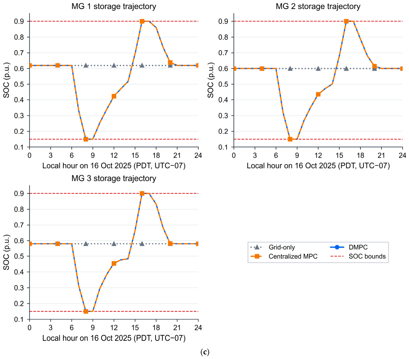
Figure 7 shows accepted DMPC dispatch and SOC trajectories over t = 0 to 24 h. SOC remains within 0.15–0.90 p.u. The maximum terminal deviation is 1.2567 × 10⁻⁶ p.u. Returning each BESS to its own initial SOC leaves the final inter-unit spread near 0.0400 p.u.; this terminal condition preserves inventory and is distinct from the primary balancing objective.

Figure 7. Accepted energy-neutral scheduling results on 16 October 2025: (a) aggregate grid-import and battery-power profiles; (b) MG1–MG3 accepted DMPC dispatch profiles; (c) MG1–MG3 SOC trajectories from t = 0 to 24 h.

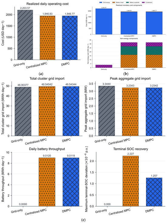
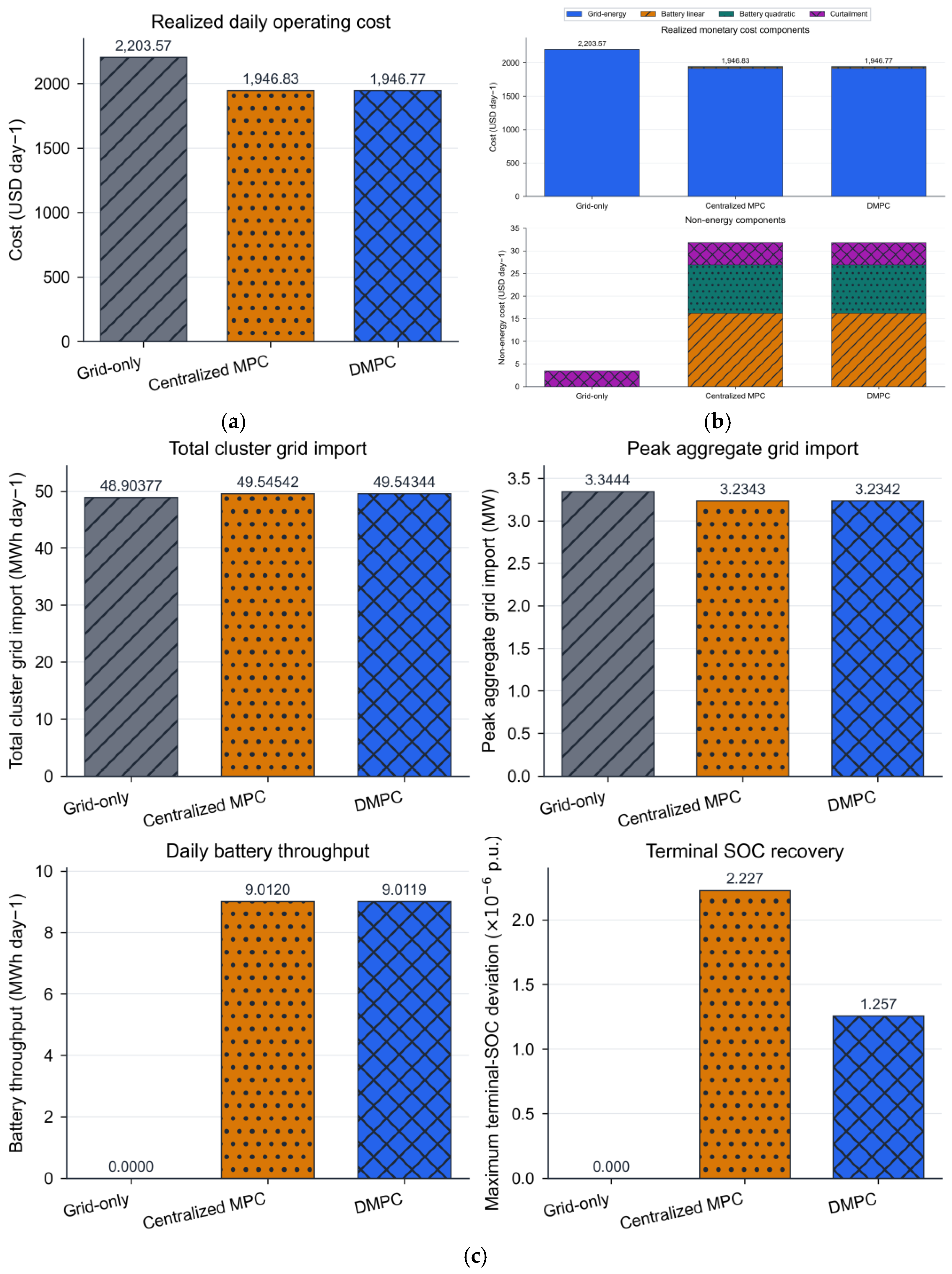
Table 2 reports original simulation results calculated using Section 5.1. Daily costs are 2203.57 USD for grid only, 1946.83 USD for centralized MPC, and 1946.77 USD for DMPC. Relative to grid only, DMPC lowers cost by 11.65% and peak aggregate import by 3.30%. Total import rises from 48.9038 to 49.5434 MWh (1.31%), and curtailment rises from 0.4405 to 0.6183 MWh. Lower expenditure therefore reflects scheduling across prices rather than lower imported energy or curtailment. The absolute centralized-DMPC realized-cost difference is 0.056653 USD, or 0.0029% of the centralized value. This observation is not an optimality bound. Terminal deviations are 1.2567 × 10⁻⁶ p.u. for DMPC and 2.2273 × 10⁻⁶ p.u. for centralized MPC.

Table 2. Original energy-neutral benchmark results on 16 October 2025 using the protocol in Section 5.1.

Strategy	Cost (USD)	Total Cluster Import (MWh)	Peak Aggregate Import (MW)	Max Terminal SOC Deviation (p.u.)
Grid-only	2203.57	48.9038	3.3444	0
Centralized MPC	1946.83	49.5454	3.2343	2.2273 × 10−6
Proposed DMPC	1946.77	49.5434	3.2342	1.2567 × 10−6

Source: authors’ simulations using the CAISO inputs [32], the configuration in Table 1, and Equation (20). These are original computed results, not values reproduced from a published comparison table.

Figure 8 compares the three benchmark strategies using the metrics defined in Section 5.1.

Figure 8. Comparison using identical data and the Section 5.1 protocol: (a) realized daily operating cost from Equation (20); (b) grid-energy, battery-throughput, quadratic-battery, and curtailment-cost components; (c) total import, peak aggregate import, battery throughput, and maximum terminal-SOC deviation. SOC regularization is excluded from monetary costs. In panels (a,c), the gray diagonal, orange dotted, and blue crosshatched bars denote the grid-only baseline, centralized MPC, and DMPC, respectively. The lower chart in panel (b) repeats the non-energy cost components on an expanded scale.

5.4. ADMM Behavior and Scalability

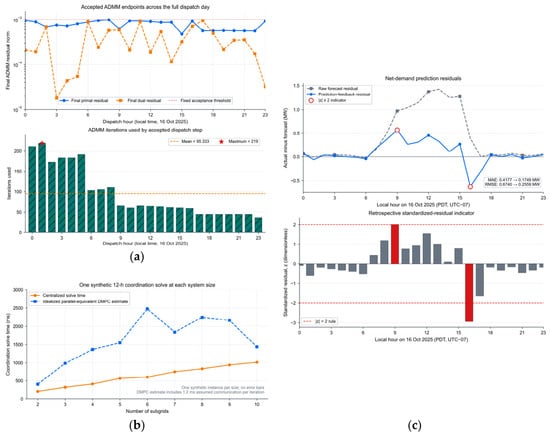
All 24 rolling DMPC steps satisfy the joint residual gate 10⁻³. Maximum final primal and dual residuals are 9.8705 × 10⁻⁴ and 9.4560 × 10⁻⁴; maximum tie-line mismatch is 6.5236 × 10⁻⁴ MW. Accepted steps use 36–219 iterations (mean 95.333). Figure 9a shows their final residuals and iteration counts. In the 2–10 node timing test, centralized MPC remains faster; at ten nodes, the centralized and parallel-equivalent DMPC solution times are 1015.5 and 1439.0 ms. The latter sums the largest local-solver time in each iteration plus an assumed 1.2 ms communication overhead per iteration. Actual network, synchronization, and deployment overheads are not measured [24,26,27,28].

Figure 9. Optimization and prediction diagnostics: (a) final residuals and iteration counts for 24 rolling solves; (b) measured centralized time and idealized parallel-equivalent DMPC time; (c) prediction residuals and retrospective standardized-residual indicators. The lower bar chart in panel (a) shows the iteration count for each rolling solve. The lower bar chart in panel (c) shows retrospective standardized prediction residuals, with red bars marking the two rule-based indicators.

Residual acceptance and the separate physical checks establish numerical feasibility within the reported tolerances. They do not certify a realized-cost optimality gap. Distribution allows local model ownership and sparse coordination, which motivate studying the architecture even without a speed advantage in this small system [26,29]. Figure 9c reports retrospective standardized prediction residuals; the two highlighted points are rule-based indicators, not a validated online fault detector.

5.5. Sensitivity Analysis Under Communication and Optimization Parameters

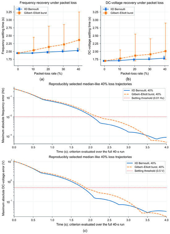
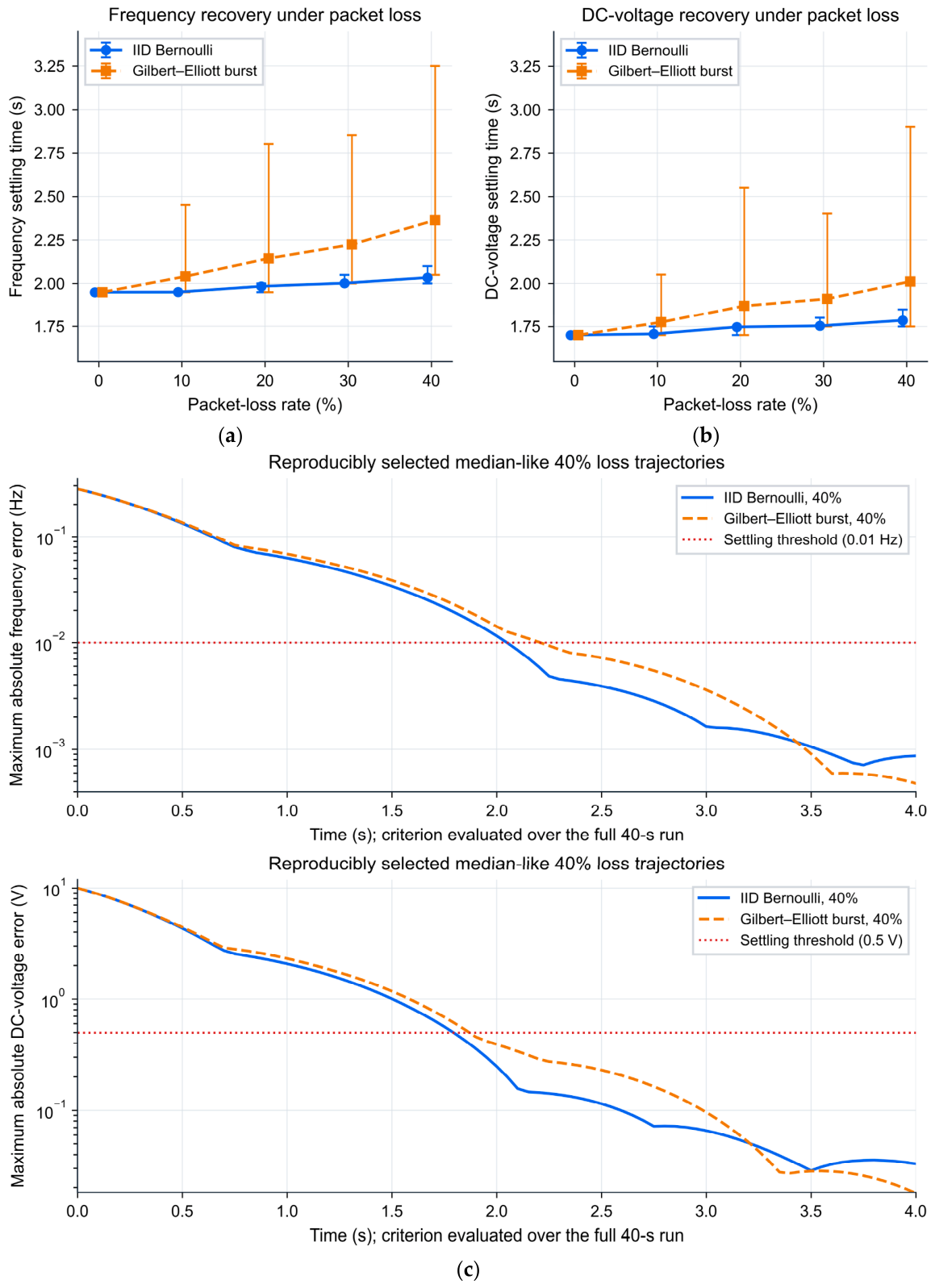
Each loss-rate/channel condition uses 200 independent seeded runs. Settling time is the earliest sample after which every node stays within 0.01 Hz or 0.5 V until 40 s; absence of that sample counts as failure. At 40% IID loss, mean settling times are 2.034 s for frequency and 1.785 s for DC voltage, with empirical 2.5th–97.5th percentile ranges [2.000, 2.100] s and [1.750, 1.850] s. Under burst loss, the means are 2.365 s and 2.012 s, with percentile ranges [2.050, 3.250] s and [1.750, 2.901] s. No run fails to settle within 40 s.

Figure 10 compares IID and two-state Gilbert–Elliott losses over 0–40%. Each directed burst channel delivers in its good state and drops in its bad state. The bad-to-good probability is 1/5 per sample; the good-to-bad probability is $p/\left[5\left(1-p\right)\right]$, giving stationary loss probability p and a mean bad-state duration of 0.25 s. Higher burst-loss rates produce wider settling-time tails. These distributions are empirical performance evidence for the configured model; Equation (19) does not prove stability of the correlated channel [18,19,20,21,22]. Markers in Figure 10a,b show mean settling times; error bars indicate the empirical 2.5th–97.5th percentiles across 200 runs per condition.

Figure 10. Packet-loss Monte Carlo results: (a) frequency settling time; (b) DC-voltage settling time; (c) representative frequency- and DC-voltage-error trajectories at 40% loss for IID Bernoulli and Gilbert–Elliott channels.

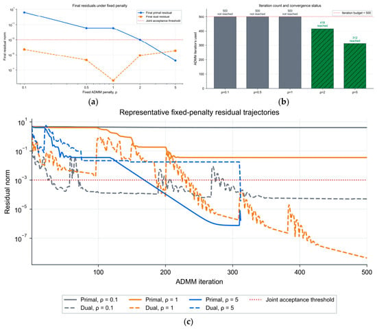
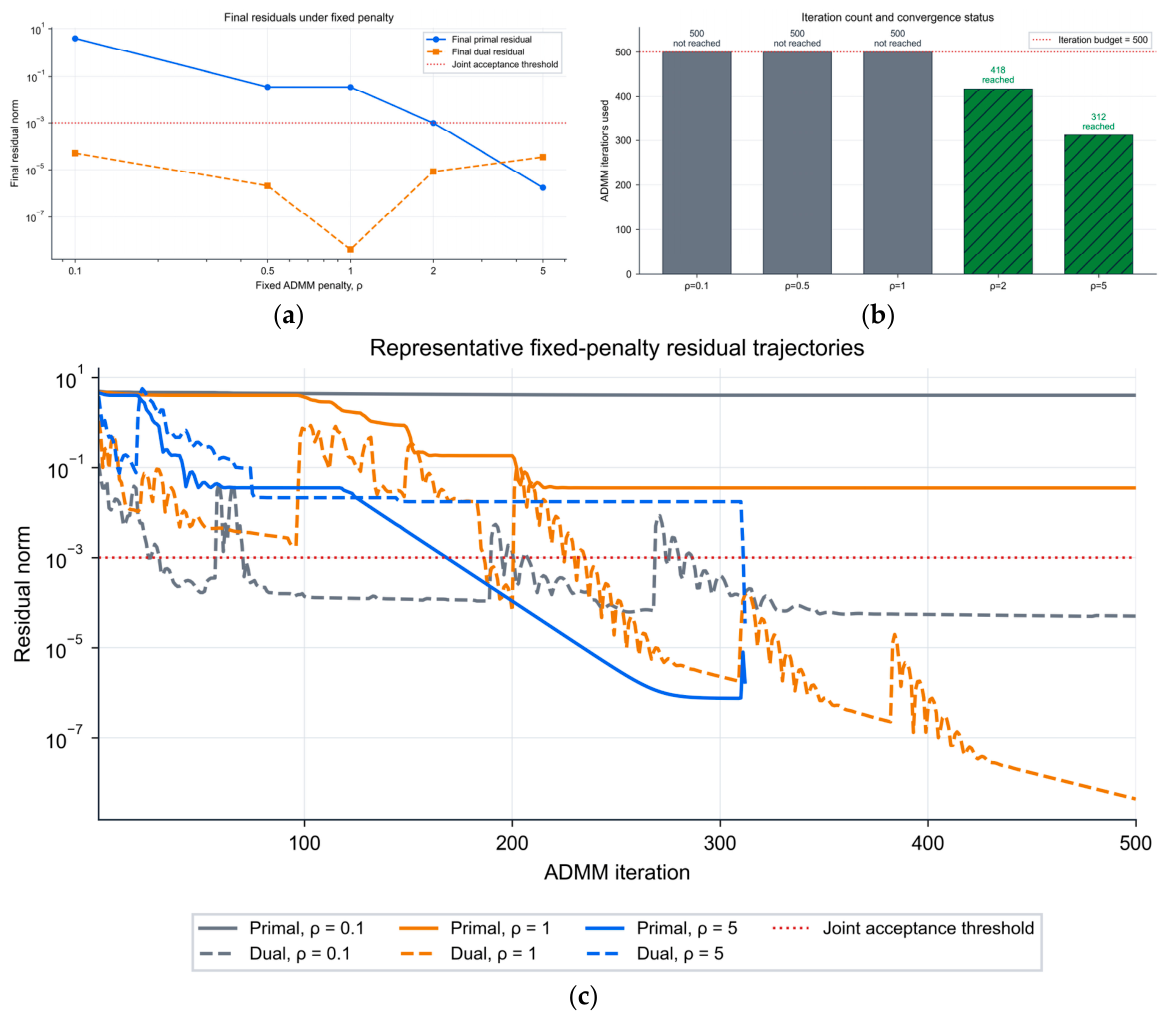
Figure 11 disables adaptive balancing and tests fixed penalties $\rho =0.1, 0.5, 1, 2, \mathrm{and} 5$ on the first 24 h coordination problem. Within 500 iterations, $\rho =0.1, 0.5, \mathrm{and} 1.0$ fail the joint gate; $\rho =2$ and $\rho =5$ pass after 418 and 312 iterations. Sensitivity to $\rho$ explains the adaptive balancing used in the main controller. This diagnostic is one coordination problem, not a full-day fixed-$\rho$ comparison [24,26,27,28].

Figure 11. Fixed-penalty ADMM sensitivity for the first coordination problem with adaptive balancing disabled: (a) final residuals; (b) iterations and acceptance; (c) representative residual trajectories.

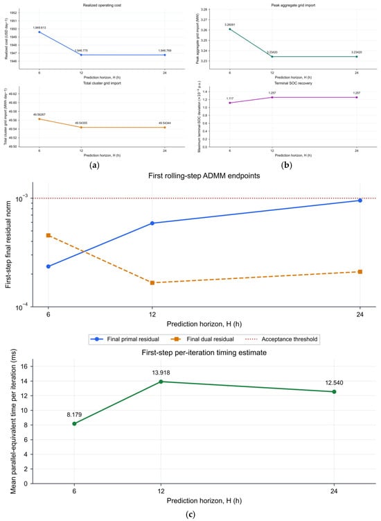
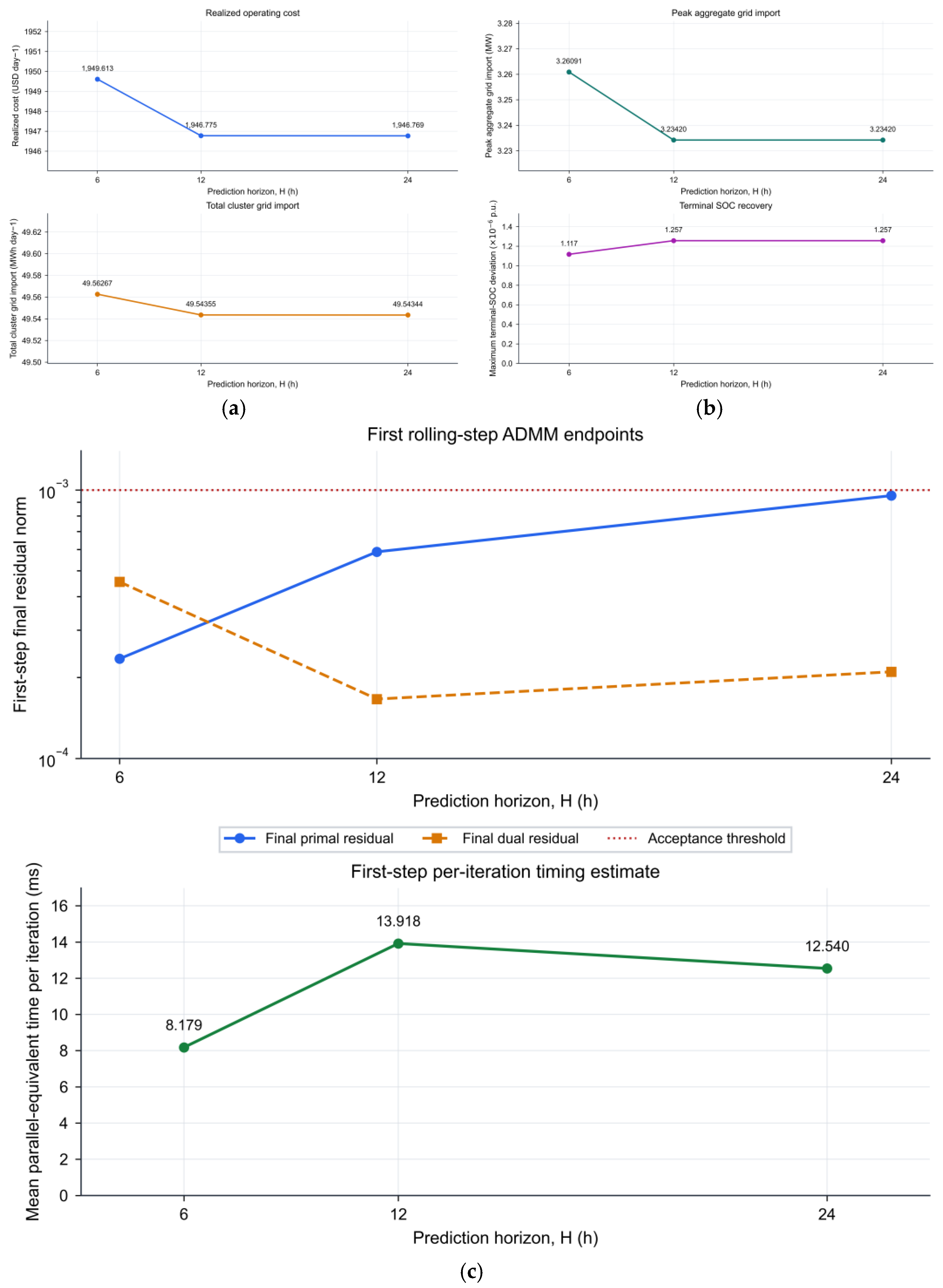
For prediction horizons 6, 12, and 24 h, daily costs are 1949.613, 1946.775, and 1946.769 USD. Total imports are 49.56267, 49.54355, and 49.54344 MWh; peak imports are 3.2609, 3.2342, and 3.2342 MW. Most of the observed economic change occurs between 6 and 12 h.

In Figure 12, maximum terminal deviations are 1.1173 × 10⁻⁶, 1.2567 × 10⁻⁶, and 1.2567 × 10⁻⁶ p.u. for H = 6, 12, and 24 h, and first-step residuals remain below 10⁻³. Mean parallel-equivalent iteration times are 8.179, 13.918, and 12.540 ms. These single-run timings are non-monotonic and do not measure deployed runtime. The principal experiment retains 24 h to cover the daily load, PV, and price cycle [23,25].

Figure 12. Prediction-horizon sensitivity: (a) realized daily operating cost and total cluster grid import; (b) peak aggregate grid import and maximum terminal-SOC deviation; (c) first-step ADMM residuals and mean parallel-equivalent time per iteration.

Table 3 summarizes the tested communication and optimization settings. It supports the stated secondary performance range and shows the sensitivity of fixed penalty $\rho$ and horizon H. Longer complete outages are evaluated separately in Section 5.8.1.

Table 3. Secondary Monte Carlo and IID stability results, fixed-penalty ADMM diagnostics, and prediction-horizon sensitivity.

Experiment	Setting	Numerical Result
IID packet loss	40%; 200 runs	$\mathrm{Frequency} 2.034 \mathrm{s} (\left[2.00,2.10\right]$); $\mathrm{DC} 1.785 \mathrm{s} (\left[1.75,1.85\right]$); failures 0/200
Burst packet loss	40%; 200 runs; mean burst 5 samples	$\mathrm{Frequency} 2.365 \mathrm{s} (\left[2.05,3.25\right]$); $\mathrm{DC} 2.012 \mathrm{s} (\left[1.75,2.901\right]$); failures 0/200
IID mean-square stability	Loss 0–40%; 24-state ZOH model	Spectral radius 0.874000–0.876193, all < 1
Fixed ADMM ρ	$\rho =0.1/0.5/1/2/5$; first 24 h problem; 500 iterations	$\rho \le 1$$\mathrm{not} \mathrm{converged}; \rho =2/5$ converged in 418/312 iterations
Prediction horizon	H = 6/12/24 h	Cost 1949.61/1946.77/1946.77 USD; peak 3.2609/3.2342/3.2342 MW

5.6. Retrospective Multi-Date Scenario and Ablation Analysis

Eight selected dates are evaluated retrospectively: 1 and 15 January, 15 and 16 April, 15 and 16 July, and 15 and 16 October 2025. The centralized equivalent uses the same objective and constraints; full distributed rolling feasibility is checked only on 16 October. The common feedback coefficient, $\alpha =0.8$, is reused after calibration on the seven dates preceding 16 October. Thus, some evaluation dates also enter calibration, and earlier scenarios use a coefficient informed by later dates. Across these selected scenarios, mean cost reduction is 9.57% (sample standard deviation 4.62%), mean peak reduction is 2.68%, and mean import increase is 1.55%. The two-date winter, spring, summer, and autumn cost-reduction means are 7.96%, 13.19%, 3.50%, and 13.61%. They are descriptive comparisons. These eight deliberately chosen dates do not support population-level inference or seasonal generalization. A causal evaluation would require a training interval preceding all target dates or calibration using only dates preceding each target.

Centralized-equivalent ablations isolate components on the selected day. The full objective gives a realized cost of 1946.83 USD. Removing prediction feedback increases it to 1995.69 USD (+2.51%); disabling tie-line exchange increases it to 2050.93 USD (+5.35%). Removing stage-SOC regularization gives 1945.98 USD (−0.043%). Prediction feedback and tie-line scheduling therefore contribute economic benefit in this case. The SOC regularizer shapes trajectories and is not demonstrated to reduce monetary cost.

5.7. Quantitative Observations

Table 4 consolidates the principal findings. It separates the primary discharge observation, the IID secondary stability result, stress-day forecast and cost metrics, and finite-tolerance optimization acceptance. The supplementary interface results follow in Section 5.8.

Table 4. Principal layer-wise findings and their interpretation.

Category	Result	Interpretation
Primary discharge	SOC gap 0.2000 to 0.1865 p.u. in 10 min	6.75% reduction in the unsaturated test
Secondary	IID spectral radius 0.874000–0.876193; 40% IID/burst failures 0/200	IID stability for the adopted autonomous model; burst evidence empirical
Forecast	MAE 0.4177 to 0.1749 MW; RMSE 0.6740 to 0.2559 MW	58.13%/62.04% reductions on the selected day
Economic scheduling	Cost −11.65%; peak −3.30%; import +1.31%; terminal deviation 1.2567 × 10−6 p.u.	Lower cost and peak with higher imported energy
Distributed optimization	24/24 accepted; max primal 0.000987051; max dual 0.000945601; cost discrepancy 0.0029%	Finite-tolerance feasibility; no certified realized-cost bound

5.8. Supplementary Outage and Cross-Layer Diagnostics

5.8.1. Complete Outages and ZOH Data Age

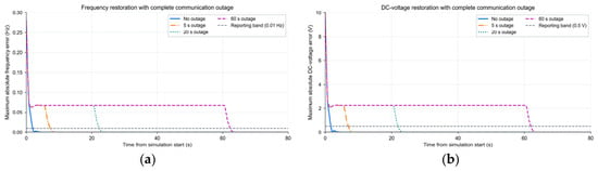
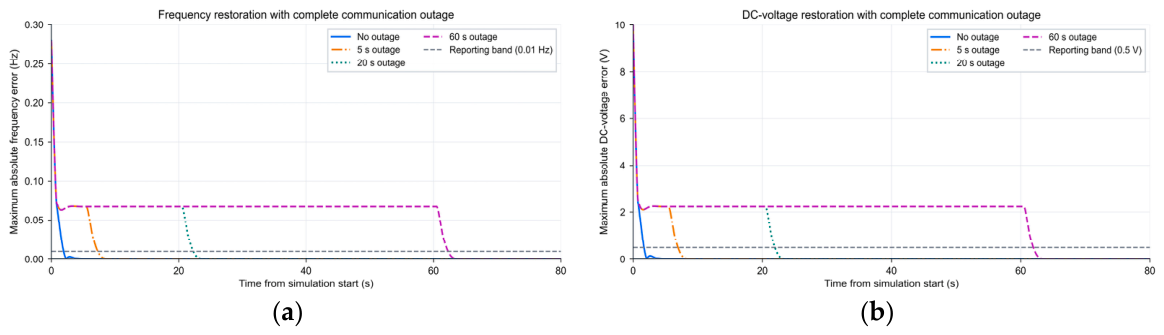
Table 5 and Figure 13 show the deterministic complete-outage experiment from Section 4.3. Without an outage, frequency and voltage settle at 1.95 and 1.70 s from initialization. With a 60 s outage beginning at 0.5 s, maximum pre-update data age is 60.05 s. Near reconnection, the worst-node errors are 0.06684 Hz and 2.23124 V; settling occurs at 62.30 and 61.95 s from initialization. Longer stale-data periods prolong a nonzero error plateau. Reconnection allows recovery for these fixed initial states and gains, but bounded trajectories in seven scenarios do not prove stability under arbitrary outages. An implementation would need timestamp monitoring, an explicitly chosen stale-data limit, and a local fallback; those safeguards are not implemented or evaluated here.

Table 5. Complete-outage results for the original autonomous secondary model.

Outage (s)	Max Data Age (s)	Error at Reconnection (Hz/V)	Settling from Start (s) Frequency/DC
0	0.05	No outage	1.95/1.70
1	1.05	0.06268/2.10324	3.25/2.90
5	5.05	0.06682/2.23072	7.30/6.95
10	10.05	0.06684/2.23124	12.30/11.95
20	20.05	0.06684/2.23124	22.30/21.95
40	40.05	0.06684/2.23124	42.30/41.95
60	60.05	0.06684/2.23124	62.30/61.95

Figure 13. Deterministic complete-outage diagnostics using the original secondary update: (a) worst-node frequency error; (b) worst-node DC-voltage error. Outages begin at 0.5 s. Dashed gray lines mark the reporting bands.

5.8.2. Persistent-Step Restoration and SOC Feedback

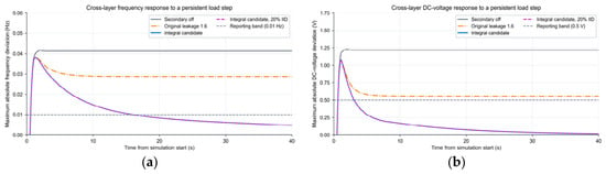
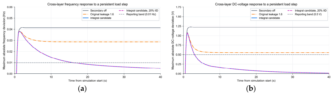
Figure 14 and Table 6 compare the reduced-order coupled variants. With secondary control disabled, final errors are 0.04130 Hz and 1.21729 V. The original leakage setting reduces these to 0.02873 Hz and 0.55637 V but does not enter both reporting bands by 40 s. Thus, its successful autonomous decay in Figure 5 does not establish persistent-load-step restoration. The integral candidate reaches the frequency and voltage bands 15.475 and 2.540 s after the step, respectively. An illustrative 20% IID realization gives 15.465 and 2.540 s, respectively. Equation (19) applies to the stand-alone model and does not prove stability of the coupled candidate.

Figure 14. Reduced-order coupled load-step diagnostic: (a) worst-node frequency deviation; (b) worst-node DC-voltage deviation. The original leakage controller and the integral candidate are distinct variants. Gray dashed lines show reporting bands; the purple dashed curve shows the candidate with one 20% IID realization.

Table 6. Reduced-order coupled persistent-step diagnostic over 40 s. Settling is measured after the 0.5 s step.

Coupled Variant	Frequency Settling (s)	DC Settling (s)	Final Error (Hz/V)
Secondary off	Not reached	Not reached	0.04130/1.21729
Original leakage 1.6	Not reached	Not reached	0.02873/0.55637
Integral candidate, no loss	15.475	2.540	0.00475/0.01796
Integral candidate, 20% IID	15.465	2.540	0.00475/0.01808

Paired post-event scheduling starts from the same actual SOC. For the integral candidate, measured-SOC feedback reduces the daily-end maximum deviation from 7.66848 × 10⁻⁵ to 1.25637 × 10⁻⁶ p.u.; its six-hour realized cost rises by 0.01657 USD. For the original leakage model, the corresponding deviations are 2.08869 × 10⁻⁴ and 1.25596 × 10⁻⁶ p.u., with a 0.02649 USD increase. These small cost changes accompany restoration of the terminal inventory. The comparison excludes the event’s incremental load cost and uses the approximate event-to-hour handoff; it is not a full daily coupled cost benchmark.

5.8.3. Combined Forecast and Communication Disturbances

All 2700 integral-candidate events in the 30-cell protocol reach the two reporting bands within 40 s. In the cell with twice the forecast error, no additional load step, and 40% burst loss, 250 runs give mean frequency settling 26.790 s and an empirical 2.5th–97.5th percentile range of 26.197–27.070 s. The matched deterministic no-loss value is 26.945 s. The percentile range includes this value, so the small difference does not show improved restoration caused by packet loss. Some larger forecast-error/step combinations recover faster because MG1’s negative residual is partly canceled by the positive load step. These cases are not evidence of monotonic disturbance rejection.

The events show no SOC or raw BESS-power violation. Tie requests activate clipping near the 0.7 MW limit, with maximum raw excess 0.000641 MW; executed tie power remains bounded. Three event-hour and 180 representative continuation solves pass both residual gates. Thirty six-hour representative continuation costs range from 855.943 to 857.087 USD. Each uses the actual sample nearest its cell’s median SOC correction. This range describes representative trajectories, not a Monte Carlo cost interval over all 2700 events. Joint results concern the documented integral extension at one event hour and do not establish robustness of the unchanged main architecture.

5.9. Limitations and Implementation Implications

The principal experiments remain layer-wise. The supplementary coupled model connects ADMM scheduling references, reduced-order fast dynamics, and event SOC feedback but uses an approximate event-to-hour energy handoff. Its primary execution preserves feasible node-specific schedules and uses SOC weighting to redistribute constrained requests; it does not continuously replace those schedules with Equation (12). The integral secondary candidate differs from the principal leakage setting. Accordingly, these experiments do not establish an end-to-end guarantee for the unchanged architecture. Persistent-step restoration of the original controller and delayed restoration during prolonged outages remain material limitations.

The data cover eight selected dates, one fully distributed daily benchmark, and one coupled event hour. The retrospective coefficient protocol cannot support causal seasonal generalization. The IID stability criterion applies to the specified autonomous linear sampled model; burst and complete-outage results are numerical observations. Averaged converter behavior omits switching transients, detailed ILC control, PCC synchronization and mode transitions, protection, and cyber-attacks. Convex throughput penalties approximate battery operating cost rather than electrochemical degradation. Distributed timing is idealized and shows no timing advantage for 2–10 nodes; the small realized-cost discrepancy is not a certified optimality bound. Deployment requires identified converter and network parameters, coordinated actuator bandwidths, communication-age supervision, fallback operation for failed solves, and hardware-in-the-loop or experimental validation. None of these deployment functions are validated here.

6. Conclusions

The study evaluates a three-layer hierarchical distributed architecture with explicit SOC accounting, ZOH receiver memory, and residual-gated energy-neutral scheduling. Capacity-aware SOC adaptation reduces the two-battery discharge gap by 6.75% after 10 min and 57.08% after 120 min under unsaturated conditions. The adopted autonomous secondary model satisfies the IID mean-square condition for tested losses up to 40%; prolonged complete outages delay restoration until communication resumes. On 16 October 2025, DMPC lowers realized cost by 11.65% and peak import by 3.30%, while imported energy increases by 1.31%. All 24 rolling solves pass the residual gate, and the realized cost differs from centralized MPC by 0.0029%. Reduced-order cross-layer diagnostics expose a persistent-step limitation in the original secondary controller; an integral candidate restores the tested deviations under combined disturbances. These analytical results and numerical observations apply within their stated assumptions. Future work requires causal multi-season data, integrated model validation, communication-age safeguards, larger deployed networks, and experimental testing.

References

- Dahane, A.S.; Sharma, R.B. Hybrid AC-DC microgrid coordinated control strategies: A systematic review and future prospect. Renew. Energy Focus 2024, 49, 100553. [Google Scholar] [CrossRef] [Scilit]
- Abdelwanis, M.I.; Elmezain, M.I. A comprehensive review of hybrid AC/DC networks: Insights into system planning, energy management, control, and protection. Neural Comput. Appl. 2024, 36, 17961–17977. [Google Scholar] [CrossRef] [Scilit]
- Sarwar, S.; Kirli, D.; Merlin, M.M.C.; Kiprakis, A.E. Major challenges towards energy management and power sharing in a hybrid AC/DC microgrid: A review. Energies 2022, 15, 8851. [Google Scholar] [CrossRef] [Scilit]
- Azeem, O.; Ali, M.; Abbas, G.; Uzair, M.; Qahmash, A.; Algarni, A.; Hussain, M.R. A comprehensive review on integration challenges, optimization techniques and control strategies of hybrid AC/DC microgrid. Appl. Sci. 2021, 11, 6242. [Google Scholar] [CrossRef] [Scilit]
- Sandeep, S.D.; Mohanty, S.; Mohanty, S.B.; Puhan, P.S. A comprehensive review on DC microgrid control and energy management strategies. Results Eng. 2025, 26, 105479. [Google Scholar] [CrossRef] [Scilit]
- Chen, B.; Wang, J.; Lu, X.; Chen, C.; Zhao, S. Networked microgrids for grid resilience, robustness, and efficiency: A review. IEEE Trans. Smart Grid 2021, 12, 18–32. [Google Scholar] [CrossRef] [Scilit]
- Olivares, D.E.; Mehrizi-Sani, A.; Etemadi, A.H.; Cañizares, C.A.; Iravani, R.; Kazerani, M.; Hajimiragha, A.H.; Gomis-Bellmunt, O.; Saeedifard, M.; Palma-Behnke, R.; et al. Trends in microgrid control. IEEE Trans. Smart Grid 2014, 5, 1905–1919. [Google Scholar] [CrossRef] [Scilit]
- Guerrero, J.M.; Vasquez, J.C.; Matas, J.; de Vicuña, L.G.; Castilla, M. Hierarchical control of droop-controlled AC and DC microgrids—A general approach toward standardization. IEEE Trans. Ind. Electron. 2011, 58, 158–172. [Google Scholar] [CrossRef] [Scilit]
- Loh, P.C.; Li, D.; Chai, Y.K.; Blaabjerg, F. Autonomous operation of hybrid microgrid with AC and DC subgrids. IEEE Trans. Power Electron. 2013, 28, 2214–2223. [Google Scholar] [CrossRef] [Scilit]
- Schiffer, J.; Ortega, R.; Astolfi, A.; Raisch, J.; Sezi, T. Conditions for stability of droop-controlled inverter-based microgrids. Automatica 2014, 50, 2457–2469. [Google Scholar] [CrossRef] [Scilit]
- Simpson-Porco, J.W.; Shafiee, Q.; Dörfler, F.; Vasquez, J.C.; Guerrero, J.M.; Bullo, F. Secondary frequency and voltage control of islanded microgrids via distributed averaging. IEEE Trans. Ind. Electron. 2015, 62, 7025–7038. [Google Scholar] [CrossRef] [Scilit]
- Bidram, A.; Davoudi, A.; Lewis, F.L.; Guerrero, J.M. Distributed cooperative secondary control of microgrids using feedback linearization. IEEE Trans. Power Syst. 2013, 28, 3462–3470. [Google Scholar] [CrossRef] [Scilit]
- Shafiee, Q.; Dragičević, T.; Vasquez, J.C.; Guerrero, J.M. Hierarchical control for multiple DC-microgrids clusters. IEEE Trans. Energy Convers. 2014, 29, 922–933. [Google Scholar] [CrossRef] [Scilit]
- Meng, L.; Dragičević, T.; Vasquez, J.C.; Guerrero, J.M. Tertiary and secondary control levels for efficiency optimization and system damping in droop controlled DC–DC converters. IEEE Trans. Smart Grid 2015, 6, 2615–2626. [Google Scholar] [CrossRef] [Scilit]
- Morstyn, T.; Hredzak, B.; Aguilera, R.P.; Agelidis, V.G. Model predictive control for distributed microgrid battery energy storage systems. IEEE Trans. Control Syst. Technol. 2018, 26, 1107–1114. [Google Scholar] [CrossRef] [Scilit]
- Chen, C.; Miao, S.; Yao, F.; Wang, T.; Wang, J.; Wei, W. Hierarchical cooperative dispatching strategy of multi-microgrid and distribution networks based on multi-agent algorithm. Autom. Electr. Power Syst. 2023, 47, 57–65. [Google Scholar] [CrossRef]
- Lou, G.; Wang, L.; Lin, D.; Du, Y.H. Review on key technologies for coordinated operation of microgrid cluster. Zhejiang Electr. Power 2025, 44, 3–19. [Google Scholar] [CrossRef]
- Li, H.; Hui, H.; Zhang, H. Consensus-based energy management of microgrid with random packet drops. IEEE Trans. Smart Grid 2023, 14, 3600–3613. [Google Scholar] [CrossRef] [Scilit]
- Yu, Y.; Liu, G.P.; Hu, W. Coordinated distributed predictive control for voltage regulation of DC microgrids with communication delays and data loss. IEEE Trans. Smart Grid 2023, 14, 1708–1722. [Google Scholar] [CrossRef] [Scilit]
- Dai, X.; Liu, G.; Hu, W.; Deng, Q.; Lei, Z. Distributed predictive control for networked DC microgrids with communication delays and packet dropouts. IEEE Trans. Ind. Inform. 2025, 21, 2294–2303. [Google Scholar] [CrossRef] [Scilit]
- Farokhi, O.; Dehkordi, N.M.; Nazaripouya, H. Robust distributed control for voltage and frequency in islanded AC microgrids with packet loss and time delay. Int. J. Electr. Power Energy Syst. 2025, 170, 110918. [Google Scholar] [CrossRef] [Scilit]
- Lai, J.; Lu, X.; Dong, Z.; Cheng, S. Resilient distributed multiagent control for AC microgrid networks subject to disturbances. IEEE Trans. Syst. Man. Cybern. Syst. 2022, 52, 43–53. [Google Scholar] [CrossRef] [Scilit]
- Parisio, A.; Rikos, E.; Glielmo, L. A model predictive control approach to microgrid operation optimization. IEEE Trans. Control Syst. Technol. 2014, 22, 1813–1827. [Google Scholar] [CrossRef] [Scilit]
- Boyd, S.; Parikh, N.; Chu, E.; Peleato, B.; Eckstein, J. Distributed optimization and statistical learning via the alternating direction method of multipliers. Found. Trends Mach. Learn. 2011, 3, 1–122. [Google Scholar] [CrossRef] [Scilit]
- Zhu, P.; Liu, Z.; Sun, K.; Wang, L.; Hu, P.; Zhu, N.; Jiang, D. Distributed model predictive control strategy based on block-wised alternating direction multiplier method for microgird clusters. IET Gener. Transm. Distrib. 2022, 16, 4630–4639. [Google Scholar] [CrossRef] [Scilit]
- Liu, G.; Ollis, T.B.; Ferrari, M.F.; Sundararajan, A.; Chen, Y. Distributed energy management for networked microgrids embedded modern distribution system using ADMM algorithm. IEEE Access 2023, 11, 102589–102604. [Google Scholar] [CrossRef] [Scilit]
- Ma, W.J.; Wang, J.; Gupta, V.; Chen, C. Distributed energy management for networked microgrids using online ADMM with regret. IEEE Trans. Smart Grid 2018, 9, 847–856. [Google Scholar] [CrossRef] [Scilit]
- Behrunani, V.N.; Cai, H.; Heer, P.; Smith, R.S.; Lygeros, J. Distributed multi-horizon model predictive control for network of energy hubs. Control Eng. Pract. 2024, 147, 105922. [Google Scholar] [CrossRef] [Scilit]
- Liu, G.; Starke, M. Networked microgrid energy management considering ownership and control structures: A comparison. Energies 2025, 18, 1115. [Google Scholar] [CrossRef] [Scilit]
- Velarde, P.; Hernández-Rivera, A.; Zafra-Cabeza, A.; Bordons, C. Cyber-resilient distributed MPC for securing microgrids against ADMM-based manipulation attacks. IFAC-PapersOnLine 2025, 59, 122–127. [Google Scholar] [CrossRef] [Scilit]
- Costa, O.L.V.; Fragoso, M.D.; Marques, R.P. Discrete-Time Markov Jump Linear Systems; Springer: London, UK, 2005. [Google Scholar] [CrossRef] [Scilit]
- California Independent System Operator. Open Access Same-Time Information System OASIS. Available online: https://www.caiso.com/systems-applications/portals-applications/open-access-same-time-information-system-oasis (accessed on 13 October 2026).
Disclaimer/Publisher’s Note: The statements, opinions and data contained in all publications are solely those of the individual author(s) and contributor(s) and not of MDPI and/or the editor(s). MDPI and/or the editor(s) disclaim responsibility for any injury to people or property resulting from any ideas, methods, instructions or products referred to in the content. |
© 2026 by the authors. Licensee MDPI, Basel, Switzerland. This article is an open access article distributed under the terms and conditions of the Creative Commons Attribution (CC BY) license.