Adaptive Range–Doppler Representation Enhancement with Lightweight Dual-View Detection for FMCW Radar Under Simulated Compound Interference

Abstract

Compound noise, clutter, and multipath reduce target–background separability in frequency-modulated continuous-wave (FMCW) radar Range–Doppler (RD) maps. Rawonly processing can leave interference-obscured weak targets insufficiently salient, whereas replacing Raw with an enhanced representation or directly mixing the two views at the input stage may attenuate useful measurement structure and introduce enhancement artifacts prematurely. To address this bottleneck, an Enhanced saliency view aligned with the original physical RD coordinates is first constructed using local median background estimation, median absolute deviation (MAD) normalization, and adaptive zero-Doppler weighting. Raw is then retained as the primary observation and encoded in parallel with Enhanced by two independent shallow branches, avoiding premature information mixing. Finally, their stride-four features are concatenated and projected through a 1 × 1 convolution to realize lightweight late fusion of the original RD structure and local target saliency. Three independently generated simulation datasets are used: Dataset A for model development, and Datasets B and C for repeated evaluation with five training seeds per dataset. Compared with the Raw baseline, Raw–Enhanced increases the mean F1 score from 0.8347 to 0.8470, corresponding to a relative improvement of 1.47%, and increases recall from 0.7470 to 0.7662 while maintaining essentially unchanged precision. The conditional range and velocity RMSEs over successfully matched detections decrease by 11.71% and 13.05%, respectively. With 10,793 trainable parameters and 27.33 MFLOPs, the proposed detector is suitable for lightweight single-frame 77 GHz one-transmitter/one-receiver FMCW moving-target range–velocity detection in complex noise, clutter, and multipath backgrounds.

1. Introduction

Frequency-modulated continuous-wave (FMCW) millimeter-wave radar senses target range and radial velocity from beat-frequency and inter-chirp phase information. A Range–Doppler (RD) representation provides a common two-dimensional organization of range and velocity information and is widely used for moving-target detection in controlled industrial and intelligent-sensing applications [1,2,3,4,5,6,7]. In complex environments, additive white Gaussian noise (AWGN) raises the background noise floor, while static and micro-motion clutter forms a nonuniform energy ridge around zero Doppler [8,9]. Multipath propagation can generate range-displaced ghost responses with Doppler characteristics similar to those of the corresponding direct target [10,11,12], and multiple targets may overlap because of finite range–velocity resolution. These compound effects reduce target–background separability, increase false and missed detections, and perturb range and velocity estimation. This study focuses on moving-target detection from a single simulated 77 GHz one-transmitter/one-receiver (1T1R) FMCW RD frame.

Existing RD target-detection methods mainly include constant-false- alarm-rate processing, deep-learning-based detection, and deterministic interference mitigation or enhancement. Cell-averaging constant false alarm rate (CA-CFAR) and ordered-statistic constant false alarm rate (OS-CFAR) provide interpretable decision rules, but their local-background assumptions can fail near clutter edges and interfering peaks [13,14,15,16]. Deep-learning-based radar processing can learn nonlinear features from RD maps, radar tensors, and micro-Doppler representations, although its performance depends on the training distribution and the selected input representation [17,18,19,20,21,22]. Deterministic interference mitigation and saliency enhancement can improve target visibility [23,24,25,26,27], but background subtraction, normalization, and suppression may also attenuate weak targets, distort useful amplitude relationships, or emphasize artifacts. A key representation bottleneck therefore remains under compound interference: Raw RD alone may provide insufficient target saliency, replacing Raw with Enhanced may discard useful scene structure, and direct input-level mixing may obscure the distinct statistics of the two representations. The central problem addressed in this study is how to exploit Enhanced target saliency while retaining the structural information carried by Raw.

To address this problem, deterministic RD enhancement is reformulated from a replacement operation into the construction of a physically aligned auxiliary representation. First, an Enhanced saliency view is generated from Raw using local median background estimation, median absolute deviation (MAD) normalization, and frame-adaptive zero-Doppler weighting. Raw and Enhanced are then encoded by two independent lightweight shallow branches based on depthwise-separable convolutions [28,29], which preserve their distinct structural and saliency characteristics before fusion. Their stride-four feature maps are subsequently concatenated and projected through a $1\times 1$ convolution, followed by multiscale center and offset heads that estimate target range, radial velocity, and confidence. Three independently generated simulation datasets are used: Dataset A for model development, and Datasets B and C for repeated evaluation with five training seeds per dataset. Compared with the single-channel Raw baseline, Raw–Enhanced increases the mean F1 score from 0.8347 to 0.8470, corresponding to a relative improvement of 1.47%, and increases recall from 0.7470 to 0.7662. The conditional range and velocity RMSEs over successfully matched detections decrease by 11.71% and 13.05%, respectively. The resulting detector contains 10,793 trainable parameters and requires 27.33 MFLOPs.

The main contributions of this study are as follows:

(1)

A controllable complex-baseband FMCW simulation framework is developed to generate direct-target echoes, additive white Gaussian noise (AWGN), static or micro-motion clutter, multipath responses, and multiple-target interference jointly in the analog-to-digital-converter domain. The resulting compound interference therefore emerges through a common Range–Doppler processing chain, providing a traceable basis for representation evaluation.

(2)

A non-learning adaptive Range–Doppler enhancement method is proposed by combining local background estimation, robust median absolute deviation normalization, and adaptive zero-Doppler weighting. The method generates an auxiliary saliency representation without changing the physical Range–Doppler coordinates, thereby reformulating enhancement from a replacement of Raw into a complementary Raw–Enhanced representation.

(3)

A lightweight dual-branch late-fusion detector is constructed to encode Raw and Enhanced independently before feature-level fusion. Raw and Enhanced single-view baselines, an equal-capacity Raw–Raw control, and the Raw–Enhanced dual-view model are evaluated using multiple training seeds on three independently generated simulation datasets to quantify the effects of complementary representations on detection completeness and range–velocity localization.

2. Related Work

2.1. FMCW Radar and Range–Doppler Processing

FMCW radar obtains range from dechirped beat frequency and velocity from inter-chirp phase progression. Reviews and baseband implementations relate waveform and sampling choices to fast-/slow-time processing [1,2]; phase noise can further alter the spectral response [30]. RD processing has supported coherent pedestrian separation [3], low-complexity FMCW detection [4], outdoor moving-target sensing [5], and Keystone-corrected vehicle detection [31]. Calibration, simulation-limit, and high-speed-object studies also demonstrate the dependence of performance on radar configuration and target state [6,7,32]. Accordingly, the present simulator states its signal and processing assumptions explicitly and retains a 1T1R single-frame task.

2.2. Classical Detection and Background Adaptation

CFAR remains an interpretable radar baseline. CA-CFAR averages training cells, whereas OS-CFAR limits the influence of strong reference cells through a ranked statistic [13]. Nonhomogeneous-background analyses explain the resulting sensitivity to clutter edges and interfering targets [14,15]; two-dimensional procedures extend the reference window over RD coordinates [16], including recent adaptations for nonuniform traffic scenes [33]. Subspace and learned clutter-suppression methods address nonstationary or millimeter-wave backgrounds [8,9], but compound scenes can still violate a single local-background model. CA-CFAR and OS-CFAR are therefore used here as conventional references, not as equivalent versions of the proposed representation approach.

2.3. Learning-Based Radar Detection

Learning-based radar processing spans RD maps, radar tensors, and micro-Doppler representations [17]. Recent work includes wavelet-based gesture recognition [18], reparameterized micro-Doppler activity recognition [19], and lightweight RD/micro-Doppler UAV processing [20]. Detection systems include RADDet on range–azimuth–Doppler tensors [21], YOLO-based FMCW detection/classification [22], YOLO-RD [34], and a compact U-Net detector for cluttered observations [35]. These tasks and inputs are not directly interchangeable. In this study, Raw and Enhanced are evaluated as single-view baselines, while an equal-capacity Raw–Raw model controls for the additional paired-view capacity. Raw–Raw and Raw–Enhanced use identical dual-branch architectures and differ only in the auxiliary input, allowing the effects of single-view representation, paired-view capacity, and Enhanced auxiliary information to be distinguished.

2.4. Interference, Clutter, and Multipath Mitigation

Interference mitigation includes waveform coordination, excision, reconstruction, filtering, and detection-stage processing [23]. Examples include phase-coded FMCW waveforms [24], environment-aware reconstruction [25], CFAR-based mitigation [26], and interference compression [27]. The present compound model instead addresses AWGN, clutter, and multipath; it does not simulate inter-radar chirp collisions.

Multipath can form plausible ghosts rather than only raising the floor. Prior work covers automotive ghost mitigation, ghost detection, measured ghost datasets, and FMCW propagation analysis [10,11,12,36]. Here, an indirect path shifts beat frequency and apparent range while retaining target Doppler. This controllable abstraction is not a full geometric propagation model.

2.5. Lightweight Detection and Representation Complementarity

Depthwise/pointwise factorization in MobileNets reduces convolutional cost [28], while MobileNetV2 adds inverted residuals and linear bottlenecks [29]. Center-based detection represents targets as heatmap peaks with regressed attributes [37]; focal loss handles sparse foreground locations [38], Smooth L1 supplies robust offset regression [39], and Adam provides the optimizer [40]. These lightweight convolutional and center-based detection components provide a compact implementation basis for the present study. Building on them, the focus is placed on whether deterministic saliency enhancement can serve as an auxiliary representation to Raw RD and how the two representations can be exploited jointly in a lightweight detector.

3. Methodology

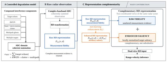
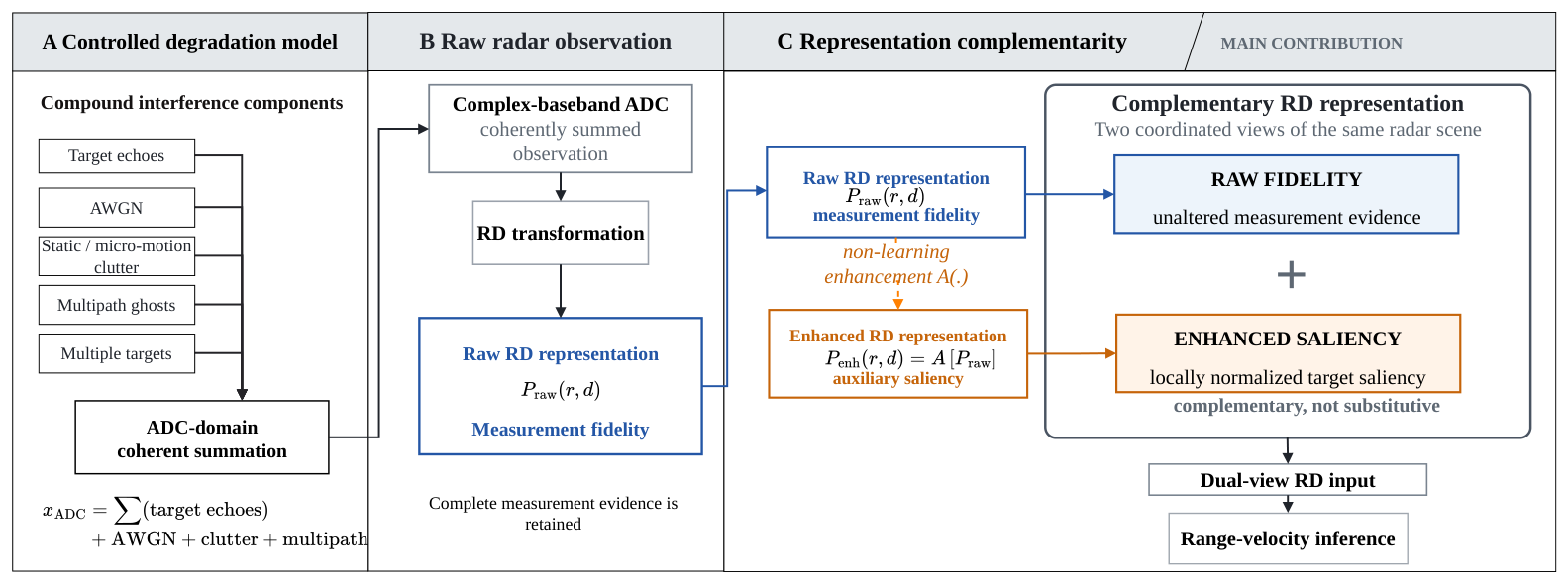
The problem considered in this study is moving-target detection from a single $256\times 128$ RD representation under compound interference. Given a Raw RD observation, the objective is to exploit an adaptive Enhanced auxiliary representation while retaining the original range–velocity structure, and to estimate target range, radial velocity, and confidence. As illustrated in Figure 1, target responses and compound interference are first generated in the ADC domain and transformed into the Raw RD representation. An Enhanced saliency representation with the same physical RD coordinates is then derived from Raw, after which a lightweight dual-view detector extracts features from the two representations independently and fuses them at a later feature stage.

Figure 1. Overall workflow of the proposed simulated FMCW Range–Doppler processing framework.

3.1. FMCW Radar Simulation Under Compound Interference

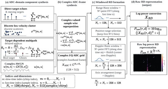
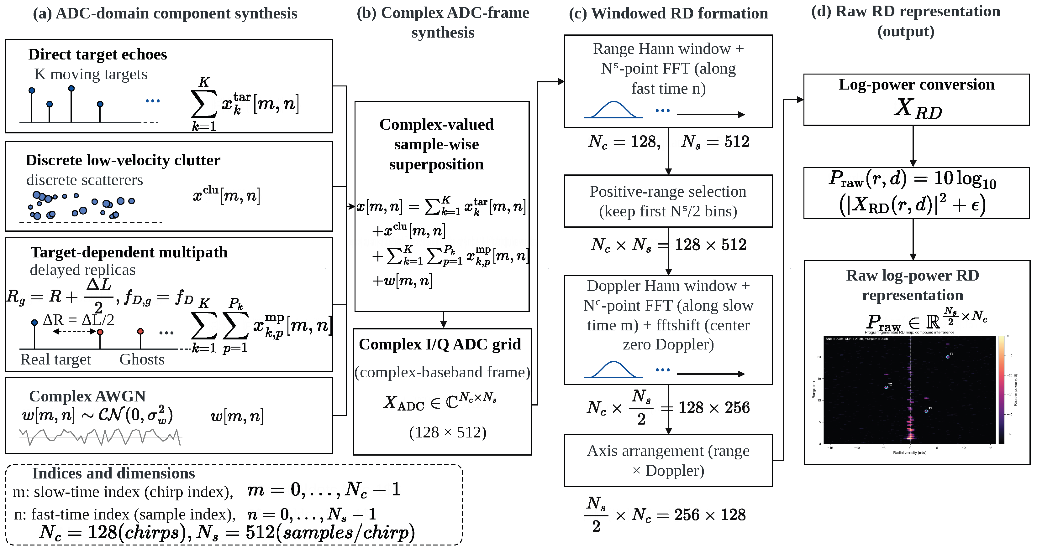
The simulation stage produces one complex-baseband analog-to-digital converter (ADC) frame for each scene. The frame contains the coherent sum of direct moving-target responses and, when enabled, additive white Gaussian noise (AWGN), static or micro-motion clutter, and multipath components. All components are generated before Range–Doppler processing. Consequently, interference affects the same windowing, Fourier transformation, power conversion, and normalization operations as the direct returns; no target, clutter, or ghost structure is inserted by modifying the RD representation. This organization provides a physics-consistent and controllable source of synthetic observations for evaluating the representation method under simulated compound interference conditions. The generation process of target and interference components is shown in Figure 2.

Figure 2. Complex-baseband simulation flow for target echoes and compound interference: (a) ADC-domain component synthesis, (b) Complex ADC-frame synthesis, (c) Windowed RD formation, and (d) Raw RD representation. All components are generated and coherently summed in the ADC domain before Range–Doppler transformation.

3.1.1. FMCW Waveform and Target Echo Model

The carrier frequency is $f_c=77\mathrm{GHz}$, and the simulated front end contains one transmitter and one receiver. Following standard FMCW baseband processing [1,2], an ideal linear FMCW chirp over the ramp interval $0\le t<T_{\mathrm{r}}$ can be written as

$$s_{\mathrm{tx}}\left(t\right)=\exp \left[j2\pi \left(f_{c}t+{\displaystyle \frac{1}{2}}S{t}^2\right)\right],S={\displaystyle \frac{B}{T_{\mathrm{r}}}},$$

(1)

where B is the sweep bandwidth, $T_{\mathrm{r}}$ is the ramp duration, and S is the chirp slope. The implemented simulator does not sample the $77\mathrm{GHz}$ radio-frequency carrier. Instead, it directly generates the dechirped complex-baseband signal that would be sampled by the ADC. This avoids an unnecessary carrier-rate simulation while retaining the beat-frequency and slow-time Doppler relationships used by the subsequent FFT processing.

Let $n\in \{0,\dots ,N_s-1\}$ denote the fast-time sample index and $m\in \{0,\dots ,N_c-1\}$ the chirp index. The corresponding time coordinates are

$$t_n={\displaystyle \frac{n}{f_s}},t_m=m{T}_c,$$

(2)

where $f_s$ is the ADC sampling frequency and $T_c$ is the chirp repetition period. For a point target k at range $R_k$ and radial velocity $v_k$, the adopted baseband approximation defines the range beat frequency and Doppler frequency as

$$f_{b,k}={\displaystyle \frac{2S{R}_k}{c}},f_{d,k}={\displaystyle \frac{2v_k}{\lambda }},\lambda ={\displaystyle \frac{c}{f_c}},$$

(3)

where c is the speed of light and $\lambda$ is the radar wavelength. Positive and negative $v_k$ values are mapped to positive and negative Doppler frequencies, respectively, according to the sign convention used throughout the simulation.

For K direct targets, the target-only ADC frame is

$$x_{\mathrm{tar}}[m,n]={\displaystyle \sum _{k=1}^K}{\alpha }_k\exp \left\{j\left[2\pi \left(f_{b,k}{t}_n+f_{d,k}{t}_m\right)+{\varphi }_k\right]\right\},$$

(4)

where ${\varphi }_k$ is an independently specified initial phase. The simulator uses a relative voltage amplitude

$${\alpha }_k={\left({\displaystyle \frac{R_{\mathrm{ref}}}{R_k}}\right)}^2\sqrt{{\displaystyle \frac{{\sigma }_k}{{\sigma }_{\mathrm{ref}}}}},{\sigma }_k={10}^{{\sigma }_{k,\mathrm{dBsm}}/10},$$

(5)

with $R_{\mathrm{ref}}=10\mathrm{m}$ and ${\sigma }_{\mathrm{ref}}=1{\mathrm{m}}^2$. This relative scaling provides range- and radar-cross-section-dependent target amplitudes without claiming a complete propagation or antenna model. The ADC matrix has shape $N_c\times N_s=128\times 512$ and is stored as complex single-precision data.

Ground-truth labels are generated directly from the prescribed $R_k$ and $v_k$ of the direct targets. Continuous range and Doppler coordinates are calculated using the same radar parameters and FFT sizes as the signal-processing chain. Interference scatterers and multipath components do not produce target labels. Thus, a range-displaced multipath peak remains an interference response even when it is locally stronger than its associated direct return. Equation (4) is a standard controllable point-target baseband model used to construct the synthetic data; it is not presented as a new FMCW signal model. The restricted ghost construction follows the range-displacement behavior examined in multipath studies [10,12,36].

3.1.2. Compound Interference Modeling

The complete simulated ADC frame is expressed as

$$x[m,n]=x_{\mathrm{tar}}[m,n]+x_{\mathrm{mp}}[m,n]+x_{\mathrm{clu}}[m,n]+w[m,n].$$

(6)

Each term can be enabled independently, while compound scenes use their coherent complex sum.

For AWGN, the noise samples follow a circular complex Gaussian distribution,

$$w[m,n]\sim \mathcal{CN}(0,{\sigma }_n^2),{\sigma }_n^2=P_{\mathrm{tar}}{10}^{-{\mathrm{SNR}}_{\mathrm{dB}}/10},$$

(7)

where $P_{\mathrm{tar}}=\mathbb{E}\left\{\right|x_{\mathrm{tar}}[m,n]{|}^2\}$ is estimated from the generated target-only frame. The real and imaginary components are independent, each with variance ${\sigma }_n^2/2$. This definition treats ${\sigma }_n^2$ as the total complex-noise power and makes the requested ADC-domain signal-to-noise ratio explicit.

Static and micro-motion clutter is represented by Q discrete scatterers,

$${\tilde{x}}_{\mathrm{clu}}[m,n]={\displaystyle \sum _{q=1}^Q}{a}_q\exp \left\{j\left[2\pi \left({\displaystyle \frac{2S{R}_q^{\left(c\right)}}{c}}{t}_n+{\displaystyle \frac{2v_q^{\left(c\right)}}{\lambda }}{t}_m\right)+{\varphi }_q^{\left(c\right)}\right]\right\}.$$

(8)

The implementation uses $20\le Q\le 100$ scatterers with ranges sampled from $1\mathrm{m}$ to the smaller of $25\mathrm{m}$ and the positive unambiguous-range limit. Their initial phases are random, and their relative strengths include a Rayleigh-distributed factor together with an $R^{-2}$ voltage dependence. Velocities are restricted to a narrow interval around zero, $v_q^{\left(c\right)}\in [-0.3,0.3]\mathrm{m}/\mathrm{s}$, thereby representing both stationary reflectors and small slow-time variations. After the raw clutter realization is generated, it is scaled to the required clutter-to-noise ratio (CNR):

$$x_{\mathrm{clu}}={\tilde{x}}_{\mathrm{clu}}\sqrt{{\displaystyle \frac{{\sigma }_n^2{10}^{{\mathrm{CNR}}_{\mathrm{dB}}/10}}{\mathbb{E}\left\{\right|{\tilde{x}}_{\mathrm{clu}}{|}^2\}}}}.$$

(9)

This scaling controls the mean complex clutter power while preserving the range, velocity, and phase structure of the discrete-scatterer realization.

Multipath ghosts are generated as additional paths associated with a direct target. For path p of target k, an extra round-trip path length $\Delta L_{k,p}$ produces the apparent range

$$R_{k,p}^{\left(\mathrm{g}\right)}=R_k+{\displaystyle \frac{\Delta L_{k,p}}{2}}.$$

(10)

The path changes the beat frequency through $R_{k,p}^{\left(\mathrm{g}\right)}$, but retains the direct target Doppler frequency $f_{d,k}$. The ghost-only contribution is

$$x_{\mathrm{mp}}[m,n]={\displaystyle \sum _{k=1}^K}{\displaystyle \sum _{p=1}^{P_k}}{\beta }_{k,p}{\alpha }_k\exp \left\{j\left[2\pi \left({\displaystyle \frac{2S{R}_{k,p}^{\left(\mathrm{g}\right)}}{c}}{t}_n+f_{d,k}{t}_m\right)+{\varphi }_k+{\psi }_{k,p}\right]\right\},$$

(11)

where ${\psi }_{k,p}$ is an additional path phase and ${\beta }_{k,p}={10}^{b_{k,p}/20}$ converts the specified voltage ratio $b_{k,p}$ from decibels to a linear scale. The implemented model allows zero to two additional paths per target, extra round-trip lengths from 1 to $12\mathrm{m}$, and amplitude ratios from $-20$ to $-3\mathrm{dB}$. It is intentionally a controlled ghost model: it captures range-displaced responses with a target-consistent Doppler coordinate but does not attempt to reproduce every geometric propagation mechanism.

Multiple direct targets are handled by the linear complex summation in Equation (4). Their responses may be resolvable, partially overlapping, or locally competing after finite-resolution FFT processing. Because target, clutter, multipath, and noise terms are combined in the ADC domain through Equation (6), the resulting RD ambiguity emerges from the common signal-processing chain rather than from image-domain editing.

3.1.3. Simulation Scope

The simulation scope is fixed to a $77\mathrm{GHz}$, 1T1R, single-frame radar and to the detection of moving targets in the range–velocity plane. One frame contains 128 chirps with 512 complex samples per chirp. The model supports controlled changes in target count, target state, AWGN level, clutter power, and multipath strength, as detailed in Section 4. The formulation excludes multiple-input multiple-output processing, angular estimation, target classification, and temporal tracking. It also does not contain measured radar data. These choices define the variables needed to test the effect of complementary RD representations while leaving spatial-array, semantic, temporal, and simulation-to-measurement questions outside the current analysis.

3.2. Range–Doppler Representation Generation

The ADC frame in Equation (6) is converted into a $256\times 128$ RD representation by a windowed two-dimensional FFT. The first dimension of the final array corresponds to positive range-frequency bins, and the second corresponds to shifted Doppler bins. The same processing is applied to every clean or interfered frame.

3.2.1. Range FFT

A symmetric Hann window is applied along fast time:

$$h_R\left[n\right]={\displaystyle \frac{1}{2}}\left[1-\cos \left({\displaystyle \frac{2\pi n}{N_s-1}}\right)\right].$$

(12)

For each chirp m, the $N_R$-point range FFT is

$$X_R[m,k]={\displaystyle \sum _{n=0}^{N_s-1}}x[m,n]h_R\left[n\right]\exp \left(-j{\displaystyle \frac{2\pi kn}{N_R}}\right),$$

(13)

where $N_R=512$. No range-domain fftshift is applied. Only $k=0,\dots ,N_R/2-1$ is retained because the implemented complex-baseband convention maps the modeled positive ranges to positive beat frequencies. The intermediate range spectrum therefore has shape $128\times 256$, indexed by chirp and range bin.

3.2.2. Doppler FFT

Before slow-time processing, a second symmetric Hann window is applied across the $N_c=128$ chirps:

$$h_D\left[m\right]={\displaystyle \frac{1}{2}}\left[1-\cos \left({\displaystyle \frac{2\pi m}{N_c-1}}\right)\right].$$

(14)

The Doppler transform of each retained range bin is

$${\tilde{X}}_{RD}[k,\mathcal{l}]={\displaystyle \sum _{m=0}^{N_c-1}}{X}_R[m,k]h_D\left[m\right]\exp \left(-j{\displaystyle \frac{2\pi \mathcal{l}m}{N_D}}\right),$$

(15)

with $N_D=128$. An fftshift is then applied only along the Doppler dimension:

$$X_{RD}[k,d]={\mathrm{fftshift}}_{\mathcal{l}}\left\{{\tilde{X}}_{RD}[k,\mathcal{l}]\right\}.$$

(16)

After arranging range as the first axis, $X_{RD}\in {\mathbb{C}}^{256\times 128}$. The zero-Doppler coordinate is $d_0=N_D/2=64$; negative and positive Doppler frequencies occupy the lower and upper halves of the shifted axis, respectively.

3.2.3. Log-Power Conversion

The combined coherent gain of the two Hann windows is

$$G=\left({\displaystyle \sum _{n=0}^{N_s-1}}{h}_R\left[n\right]\right)\left({\displaystyle \sum _{m=0}^{N_c-1}}{h}_D\left[m\right]\right).$$

(17)

The linear RD power and raw log-power representation are calculated as

$$L[k,d]={\displaystyle \frac{|X_{RD}{[k,d]|}^2}{G^2}},P[k,d]=10{\log }_{10}\left(\max \left\{L\right[k,d],ϵ\}\right),$$

(18)

where $ϵ={10}^{-12}$ is a numerical floor. $P\in {\mathbb{R}}^{256\times 128}$, expressed in decibels, is the raw RD representation used by the enhancement procedure and the detector input normalization. The coherent-gain correction makes power values comparable across frames generated with the same processing chain; it is not used to alter the locations of RD peaks.

3.2.4. Coordinate Mapping

For range bin k, the beat-frequency and distance coordinates are

$$f_b\left[k\right]={\displaystyle \frac{k{f}_s}{N_R}},R\left[k\right]={\displaystyle \frac{c{f}_s}{2S{N}_R}}k.$$

(19)

For shifted Doppler bin d, the Doppler-frequency and radial-velocity coordinates are

$$f_D\left[d\right]={\displaystyle \frac{d-N_D/2}{N_D{T}_c}},v\left[d\right]={\displaystyle \frac{\lambda }{2N_D{T}_c}}\left(d-{\displaystyle \frac{N_D}{2}}\right).$$

(20)

The continuous full-resolution bin labels associated with a target state are therefore

$$u_{R,k}={\displaystyle \frac{2S{R}_k}{c}}{\displaystyle \frac{N_R}{f_s}},u_{D,k}={\displaystyle \frac{N_D}{2}}+{\displaystyle \frac{2v_k}{\lambda }}{T}_c{N}_D.$$

(21)

For the adopted configuration, the range-bin spacing is $\Delta R=c{f}_s/\left(2S{N}_R\right)\approx 0.0976\mathrm{m}$, and the Doppler-bin spacing corresponds to $\Delta v=\lambda /\left(2N_D{T}_c\right)\approx 0.2535\mathrm{m}/\mathrm{s}$. These continuous coordinates are retained for detector-label construction so that sub-bin offsets can be learned instead of forcing every target to the nearest integer cell.

3.3. Adaptive Range–Doppler Representation Enhancement

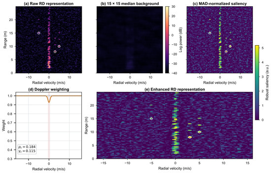
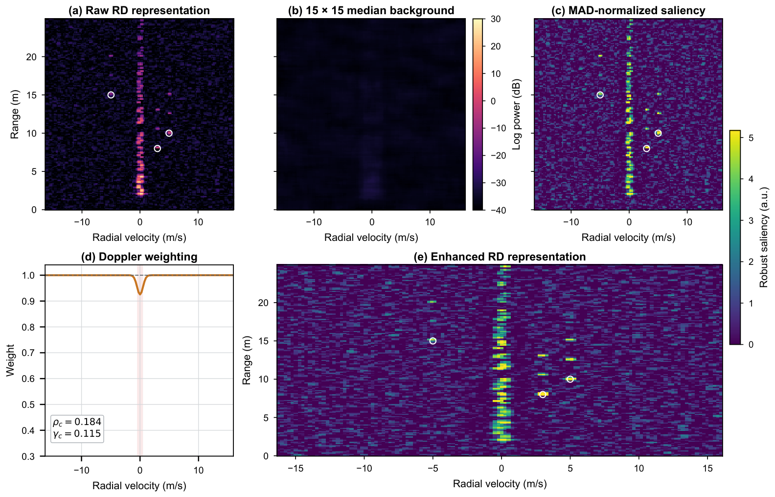
The enhancement transforms the raw log-power map P into a non-negative saliency representation E without learned parameters. It combines local background subtraction, robust local scaling, and a frame-dependent weighting around zero Doppler. Its purpose is to expose structure that may be less apparent in the raw dynamic range. Because any deterministic transform can also attenuate useful content, E is used as an auxiliary view and the original P is retained. The intermediate enhancement procedure is illustrated in Figure 3.

Figure 3. Intermediate stages of the adaptive RD representation enhancement under simulated compound interference: (a) raw RD representation, (b) local median background, (c) MAD-normalized saliency, (d) Doppler weighting, and (e) enhanced RD representation. White circles indicate direct-target coordinates, and the shaded area with the vertical dashed line represents the central Doppler band for interference weighting.

3.3.1. Local Background Estimation

For each cell $(r,d)$, a $15\times 15$ reflected neighborhood ${\mathcal{N}}_{r,d}$ is used to estimate the local background:

$$B[r,d]=\mathrm{median}\left\{P[i,j]:(i,j)\in {\mathcal{N}}_{r,d}\right\}.$$

(22)

Reflection padding is applied at the RD boundaries so that all output cells use a complete neighborhood and the output size remains $256\times 128$. The local residual is

$$D[r,d]=P[r,d]-B[r,d].$$

(23)

The median estimate is less sensitive than a local mean to a small number of high-amplitude cells. Subtracting B removes a slowly varying local offset and changes the representation from absolute log power to local contrast. It does not identify a cell as a target and does not use any ground-truth labels.

3.3.2. Robust Local Normalization

The residual magnitude is summarized over the same neighborhood:

$$M[r,d]=\mathrm{median}\left\{\left|D[i,j]\right|:(i,j)\in {\mathcal{N}}_{r,d}\right\}.$$

(24)

A Gaussian-consistent robust scale with a numerical floor is then defined as

$$s[r,d]=\max \left\{1.4826M[r,d],{10}^{-3}\right\}.$$

(25)

The normalized positive saliency is

$$Z[r,d]=\max \left\{{\displaystyle \frac{D[r,d]}{s[r,d]}},0\right\}.$$

(26)

Negative residuals are set to zero because the auxiliary view is designed to represent locally elevated responses. The factor $1.4826$ provides the conventional Gaussian-consistent scaling of a median absolute residual statistic, while the floor prevents division by a near-zero value in uniform regions. This robust local scaling normalizes residual responses across nonuniform background regions and reduces the influence of local background-amplitude variation on the saliency representation.

3.3.3. Doppler-Aware Interference Weighting

Static and micro-motion clutter tends to concentrate saliency near the shifted zero-Doppler coordinate. To adapt the suppression strength to each frame, the method first measures the proportion of positive saliency in the center Doppler band

$$\mathcal{C}=\left\{d:|d-d_0|\le 2\right\},d_0=64,$$

(27)

and computes

$${\rho }_c=\left\{\begin{array}{cc}{\displaystyle \frac{{\sum }_r{\sum }_{d\in \mathcal{C}}Z[r,d]}{{\sum }_r{\sum }_{d}Z[r,d]},}\hfill & \sum _{r,d}Z[r,d]>0,\hfill \\ 0,\hfill & \mathrm{otherwise}.\hfill \end{array}\right.$$

(28)

Although ${\rho }_c$ describes an energy-concentration tendency, it is evaluated from the non-negative saliency values rather than from the original linear RD power. The ratio is mapped to a clutter-strength coefficient

$$\gamma =clip\left({\displaystyle \frac{{\rho }_c-{\rho }_0}{{\rho }_1-{\rho }_0}},0,1\right),{\rho }_0=0.15,{\rho }_1=0.45.$$

(29)

Thus, no Doppler attenuation is introduced when ${\rho }_c\le {\rho }_0$, while the maximum configured attenuation is reached when ${\rho }_c\ge {\rho }_1$.

A Gaussian profile localizes the weighting around zero Doppler:

$$g\left[d\right]=\exp \left[-{\displaystyle \frac{{(d-d_0)}^2}{2{\sigma }_d^2}}\right],{\sigma }_d=2,$$

(30)

and the final one-dimensional weight is

$$w\left[d\right]=1-\gamma (1-w_{\min })g\left[d\right],w_{\min }=0.35.$$

(31)

The weight approaches one outside the central band. Near $d_0$, it is reduced only when the frame contains a sufficiently high zero-Doppler saliency ratio. This design targets the static or micro-motion clutter pattern represented by the simulator without imposing a fixed amount of suppression on every frame.

3.3.4. Enhanced Representation

The enhanced RD representation is

$$E[r,d]=Z[r,d]w\left[d\right].$$

(32)

It has the same $256\times 128$ coordinate system as P, contains no negative values, and is stored in single precision. Equations (22)–(32) contain no learned parameter. The transformation can improve the visibility of a locally distinctive target response when the raw background is uneven or dominated by near-zero-Doppler clutter. However, the clipping and Doppler weighting can also remove or attenuate information. The enhanced RD representation is therefore defined as a complementary representation and does not replace the raw RD representation.

3.4. Lightweight Detector for Complementary RD Representations

A common lightweight detector framework is used to evaluate and exploit the complementary information carried by the Raw and Enhanced RD representations. The Raw and Enhanced single-view models use the same compact depthwise-separable encoder and differ only in their input representation. Raw–Raw and Raw–Enhanced instead use the same dual-branch late-fusion architecture. Raw–Enhanced uses Enhanced as the auxiliary view, whereas Raw–Raw supplies a duplicate Raw representation to the auxiliary branch, providing an equal-capacity control for the paired-view design.

3.4.1. Dual-View Input

Before feature extraction, the raw log-power map is normalized over a $60\mathrm{dB}$ per-frame dynamic range:

$$X_{\mathrm{raw}}[r,d]=clip\left({\displaystyle \frac{P[r,d]-P_{\max }+60}{60}},0,1\right),P_{\max }=\underset{r,d}{\max }P[r,d].$$

(33)

The enhanced RD representation is normalized by its frame-wise $99.9$th percentile:

$$X_{\mathrm{enh}}[r,d]=clip\left({\displaystyle \frac{E[r,d]}{\max \{Q_{99.9}\left(E\right),{10}^{-6}\}}},0,1\right),$$

(34)

where $Q_{99.9}\left(E\right)$ denotes the $99.9$th percentile of the enhanced frame. The normalized Raw and Enhanced representations share the same $256\times 128$ physical coordinate system. The single-view Raw and Enhanced models receive $X_{\mathrm{raw}}$ and $X_{\mathrm{enh}}$, respectively, as their sole input. For Raw–Enhanced, the primary branch receives $X_{\mathrm{raw}}$ and the auxiliary branch receives $X_{\mathrm{enh}}$. For the equal-capacity Raw–Raw control, both branches receive $X_{\mathrm{raw}}$. The two paired-view models therefore have identical trainable architectures and differ only in the representation supplied to the auxiliary branch.

3.4.2. Lightweight Backbone

The basic operator is a depthwise-separable convolution, following the efficient factorization used in lightweight convolutional networks [28,29]. For an input feature tensor with $C_{\mathrm{in}}$ channels, a $3\times 3$ depthwise convolution independently filters each channel, after which a $1\times 1$ pointwise convolution projects the features to $C_{\mathrm{out}}$ channels. Batch normalization and a rectified linear unit follow both convolutional operations. This factorization reduces the number of parameters relative to a dense $3\times 3$ convolution while preserving local spatial processing.

The single-view Raw baseline retains a four-stage lightweight depthwise-separable encoder. For the paired-view models, Raw and the auxiliary representation are processed by two independent shallow branches covering the first two encoder stages. Each branch produces a stride-four feature map with 16 channels and spatial size $64\times 32$. Denoting the two features by ${\mathbf{F}}_2^R$ and ${\mathbf{F}}_2^A$, they are concatenated along the channel dimension and projected from 32 to 16 channels:

$${\mathbf{F}}_2=\mathrm{ReLU}\left(\mathrm{BN}\left(W_{1\times 1}\ast [{\mathbf{F}}_2^R,{\mathbf{F}}_2^A]\right)\right).$$

(35)

The fused feature is subsequently processed by the shared third and fourth encoder stages. For multiscale aggregation, the stride-four fine-scale feature and the stride-sixteen coarse feature are independently projected to 24 channels. The coarse feature is bilinearly upsampled to $64\times 32$, concatenated with the fine-scale feature, and processed by a depthwise-separable fusion block to produce the final 24-channel detection feature. This late-fusion design delays cross-view interaction until the Raw structural features and auxiliary saliency features have been independently encoded. The single-channel Raw detector contains 9334 trainable parameters, whereas both Raw–Raw and Raw–Enhanced contain 10,793 trainable parameters.

3.4.3. Detection Heads

Two parallel heads operate on the fused $24\times 64\times 32$ feature map. The center head uses a depthwise-separable 24-to-16-channel block followed by a $1\times 1$ convolution to produce heatmap logits

$$\widehat{\mathbf{H}}\in {\mathbb{R}}^{1\times 64\times 32}.$$

(36)

The offset head uses the same channel pattern followed by a two-channel $1\times 1$ convolution and a sigmoid function:

$$\widehat{\mathbf{O}}\in {[0,1]}^{2\times 64\times 32}.$$

(37)

The two offset channels encode the fractional range and Doppler positions within each output cell. The bias of the final heatmap convolution is initialized to $-2.19$, which reduces the initial foreground probability.

The output stride is $s_o=4$. For a target with continuous full-resolution bins $(u_R,u_D)$ from Equation (21), its output-grid center and offset labels are

$$i=⌊{\displaystyle \frac{u_R}{s_o}}⌋,j=⌊{\displaystyle \frac{u_D}{s_o}}⌋,{\mathbf{o}}_{i,j}=\left[\begin{array}{c}{u}_R/s_o-i\\ u_D/s_o-j\end{array}\right].$$

(38)

A radius-one Gaussian is drawn around each center in the target heatmap, and the offset loss is activated only at the integer center cell. At inference, a sigmoid converts the heatmap logits to confidence values. Local maxima are selected using $3\times 3$ max pooling, after which thresholding and top-K selection are applied as specified in Section 4. A detected center $(i,j)$ is decoded as

$${\widehat{u}}_R=s_o(i+{\widehat{O}}_R[i,j]),{\widehat{u}}_D=s_o(j+{\widehat{O}}_D[i,j]).$$

(39)

Equations (19) and (20) then convert the decoded bins to range and radial velocity. The heatmap probability at the selected center is reported as detection confidence.

3.4.4. Training Objective

The training objective combines a center-based focal loss, a masked Smooth L1 offset-regression loss, and a lightweight background-peak penalty. The center representation follows the heatmap-and-offset formulation of point-based detection [37], the heatmap term follows the focal-loss principle for sparse foreground locations [38], and the offset term uses the piecewise Smooth L1 formulation [39].

Let $H_{i,j}\in [0,1]$ denote the Gaussian target heatmap and ${\widehat{p}}_{i,j}=\mathrm{sigmoid}\left({\widehat{H}}_{i,j}\right)$ the predicted center probability. With $\alpha =2$, $\beta =4$, and $N_p$ denoting the number of positive target centers, the heatmap loss is

$${\mathcal{L}}_{\mathrm{hm}}=-{\displaystyle \frac{1}{\max \{N_p,1\}}}\left[\sum _{H_{i,j}=1}{(1-{\widehat{p}}_{i,j})}^{\alpha }\log {\widehat{p}}_{i,j}+\sum _{H_{i,j}<1}{(1-H_{i,j})}^{\beta }{\widehat{p}}_{i,j}^{\alpha }\log (1-{\widehat{p}}_{i,j})\right].$$

(40)

The probabilities are numerically clipped to $[{10}^{-6},1-{10}^{-6}]$ before evaluating the logarithms.

Let $M_{i,j}$ be one at labeled center cells and zero elsewhere, and denote the offset residual by ${\epsilon }_{c,i,j}={\widehat{O}}_{c,i,j}-O_{c,i,j}$ for $c\in \{1,2\}$. The masked offset-regression loss is

$${\mathcal{L}}_{\mathrm{off}}={\displaystyle \frac{{\sum }_{c,i,j}{M}_{i,j}{\mathrm{smooth}}_{L_1}\left({\epsilon }_{c,i,j}\right)}{\max \left\{{\sum }_{c,i,j}{M}_{i,j},1\right\}}}.$$

(41)

where

$${\mathrm{smooth}}_{L_1}\left(\epsilon \right)=\left\{\begin{array}{cc}{\displaystyle \frac{1}{2}}{\epsilon }^2,\hfill & \left|\epsilon \right|<1,\hfill \\ \left|\epsilon \right|-{\displaystyle \frac{1}{2}},\hfill & \mathrm{otherwise}.\hfill \end{array}\right.$$

(42)

To suppress high-confidence background peaks, an additional background-peak penalty is applied during training. Let $B_{i,j}$ be one at $3\times 3$ local maxima whose target-heatmap value is below 0.1 and zero elsewhere. The penalty is

$${\mathcal{L}}_{\mathrm{fp}}={\displaystyle \frac{{\sum }_{i,j}{B}_{i,j}{\widehat{p}}_{i,j}}{\max \left\{{\sum }_{i,j}{B}_{i,j},1\right\}}}.$$

(43)

The final training objective is

$$\mathcal{L}={\mathcal{L}}_{\mathrm{hm}}+0.5{\mathcal{L}}_{\mathrm{off}}+0.05{\mathcal{L}}_{\mathrm{fp}}.$$

(44)

The same objective and loss weights are used for Raw, Enhanced, Raw–Raw, and Raw–Enhanced.

4. Experiments and Results

4.1. Experimental Setup and Reproducibility

4.1.1. Radar and Scenario Configuration

All experiments used the $77\mathrm{GHz}$, one-transmitter/one-receiver (1T1R), single-frame FMCW configuration defined in Section 3.1. The radar, scene, dataset, training, and evaluation settings are summarized in Table 1. The transmitted bandwidth was $1.536\mathrm{GHz}$, the ramp duration was $51.2\mathsf{\mu }\mathrm{s}$, and the chirp repetition period was $60\mathsf{\mu }\mathrm{s}$. Each chirp contained 512 complex-baseband ADC samples acquired at $10\mathrm{MHz}$, and each frame contained 128 chirps. A 512-point range FFT and a 128-point Doppler FFT produced a $256\times 128$ positive-range RD representation. These values correspond to a range-bin spacing of approximately $0.0976\mathrm{m}$ and a velocity-bin spacing of approximately $0.2535\mathrm{m}/\mathrm{s}$.

Table 1. Simulation, dataset, training, and evaluation settings.

Group	Parameter	Value or Distribution
Radar	Carrier frequency/channels	77 GHz/1T1R
Radar	Bandwidth/ramp duration	1.536 GHz/51.2 $\mathsf{\mu }$s
Radar	Chirp period/sampling rate	60 $\mathsf{\mu }$s/10 MHz
Radar	Samples per chirp/chirps per frame	512/128
Radar	Range FFT/Doppler FFT/RD size	512/128/$256\times 128$
Target	Number/range/$\left|v\right|$	1–5/2–23 m/0.5–12 m/s
Target	RCS/initial phase	$[-10,10]$ dBsm/$[0,2\pi )$
Interference	SNR/CNR	$[-15,15]$ dB/$[0,30]$ dB
Interference	Clutter scatterers	20–100; velocity in $[-0.3,0.3]$ m/s
Interference	Multipath paths/amplitude ratio	0–2 per target/$[-20,-3]$ dB
Interference	Additional round-trip path length	1–12 m
Dataset	Datasets	A, B, and C independently generated simulation datasets
Dataset	Frames per dataset (train/validation/test)	5000/1000/2000
Dataset	Master seeds (A/B/C)	20260722/30260722/40260722
Dataset	Split offsets (train/validation/test)	0/50,000/60,000
Dataset	Frame-seed increment	10
Model	Paired-view fusion	Dual-branch late fusion with $1\times 1$ projection
Model	Single-view inputs	Raw/Enhanced
Model	Paired-view inputs	Raw–Raw/Raw–Enhanced
Training	Training seeds	42, 123, 2026, 3407, 5208
Training	Optimizer/epochs/batch size	Adam/30/32
Training	Learning rate/weight decay	${10}^{-3}$/${10}^{-5}$
Training	Training objective	${\mathcal{L}}_{\mathrm{hm}}+0.5{\mathcal{L}}_{\mathrm{off}}+0.05{\mathcal{L}}_{\mathrm{fp}}$
Evaluation	Confidence threshold	0.45
Evaluation	Top-K	10
Evaluation	Matching gate	4 range bins and 4 Doppler bins

The dataset contained only simulated complex-baseband radar frames. For each frame, the number of direct moving targets was sampled uniformly from one to five. Target range was sampled from 2 to $23\mathrm{m}$, the magnitude of radial velocity from $0.5$ to $12\mathrm{m}/\mathrm{s}$, and the sign of velocity with equal probability. Radar cross section (RCS) was uniformly sampled from $-10$ to $10\mathrm{dBsm}$, while the initial phase was uniformly distributed over $[0,2\pi )$. Direct-target labels were generated from the sampled physical range and velocity. Multipath components were not assigned target labels.

Compound interference was generated in the complex ADC domain before either FFT. The signal-to-noise ratio (SNR) was uniformly sampled from $-15$ to $15\mathrm{dB}$. Each clutter realization contained 20–100 static or micro-motion scatterers with a clutter-to-noise ratio (CNR) between 0 and $30\mathrm{dB}$. Zero, one, or two multipath components were generated per direct target; their amplitude ratios were sampled from $-20$ to $-3\mathrm{dB}$ and their additional propagation lengths from 1 to $12\mathrm{m}$ subject to the unambiguous-range limit. The direct echoes of all sampled targets, multipath echoes, clutter, and additive white Gaussian noise (AWGN) were then coherently added. Thus, the interference affected the RD representation through the same signal-processing chain as the direct targets rather than through an image-domain perturbation.

4.1.2. Dataset Construction and Detector Training

Three independently generated simulation datasets, denoted A, B, and C, were constructed using different master random seeds. Each dataset contains 5000 training, 1000 validation, and 2000 test frames while sharing the same radar configuration, target ranges, and compound- interference distributions. Dataset A was used for architecture, training-configuration, and confidence-threshold selection, whereas Datasets B and C were used for repeated performance evaluation.

Several lightweight dual-view fusion alternatives were compared using the training and validation data of Dataset A, and the dual-branch late-fusion structure was selected. All compared models used the Adam optimizer [40], a learning rate of ${10}^{-3}$, weight decay of ${10}^{-5}$, batch size 32, and 30 training epochs. For the final evaluation, Raw, Enhanced, Raw–Raw, and Raw–Enhanced were independently trained on Datasets B and C using five training seeds (42, 123, 2026, 3407, and 5208), resulting in 40 repeated training runs.

4.1.3. Evaluation Protocol

A common confidence threshold of 0.45 was selected using Dataset A validation data and fixed before evaluation on Datasets B and C. At most ten local maxima were retained per frame. Predicted and true target centers were greedily associated within a gate of four range bins and four Doppler bins, with each prediction and target participating in at most one match. A matched pair was counted as a true positive (TP), an unmatched prediction as a false positive (FP), and an unmatched target as a false negative (FN). Precision, recall, and F1 were calculated as

$$\mathrm{Precision}={\displaystyle \frac{\mathrm{TP}}{\mathrm{TP}+\mathrm{FP}}},\mathrm{Recall}={\displaystyle \frac{\mathrm{TP}}{\mathrm{TP}+\mathrm{FN}}},$$

(45)

$$\mathrm{F}1={\displaystyle \frac{2\mathrm{Precision}\mathrm{Recall}}{\mathrm{Precision}+\mathrm{Recall}}}.$$

(46)

Detection probability, denoted by $P_{\mathrm{d}}$, was defined as the fraction of test frames containing at least one matched target. Because each simulated frame contained at least one target, this frame-level quantity measured whether a method produced any valid target detection; precision, recall, and F1 remained necessary for evaluating multi-target completeness and false alarms.

For the $N_{\mathrm{TP}}$ matched target–prediction pairs, range and velocity localization errors were reported as

$${\mathrm{RMSE}}_R=\sqrt{{\displaystyle \frac{1}{N_{\mathrm{TP}}}}\sum _{i=1}^{N_{\mathrm{TP}}}{\left({\widehat{R}}_i-R_i\right)}^2},{\mathrm{RMSE}}_v=\sqrt{{\displaystyle \frac{1}{N_{\mathrm{TP}}}}\sum _{i=1}^{N_{\mathrm{TP}}}{\left({\widehat{v}}_i-v_i\right)}^2}.$$

(47)

The range and velocity RMSEs are computed over the successfully matched targets of each detector. Because different methods may produce different matched-target sets, these metrics quantify localization error conditional on successful detection rather than paired localization error over an identical target subset.

The physical errors were obtained from the continuous decoded bin coordinates using the range and velocity mappings in Section 3.2. For each evaluation dataset, detector results are reported as the mean ± sample standard deviation over five training seeds. For the Across B–C summary, the five runs are first averaged within each dataset and the two dataset-level means are then summarized. The ten training runs are therefore not treated as ten independent dataset replicates. Within each dataset, the reported standard deviation reflects variability due to training initialization and minibatch ordering. For the Across B–C summary, the variability instead reflects the two dataset-level means. Neither quantity should be interpreted as a confidence interval over a population of measured radar datasets.

4.2. Verification of FMCW Simulation and Interference Models

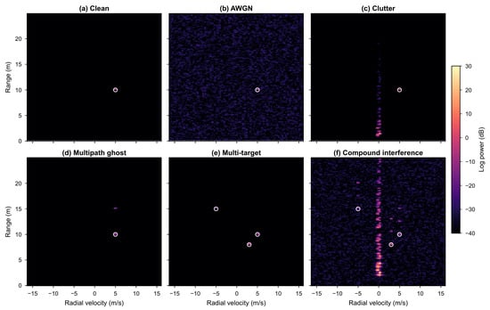
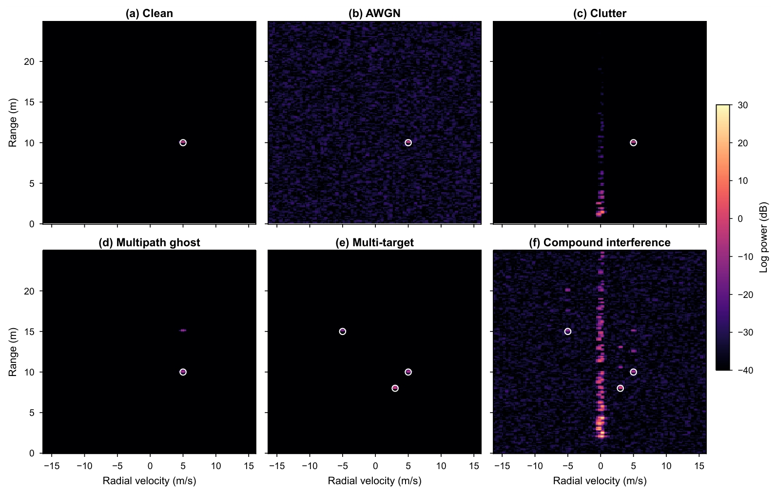
Before generating the detection datasets, the numerical simulator was verified against the analytic signal relationships for beat and Doppler frequency, AWGN power, clutter distribution, and multipath peak location. Representative RD degradations under different interference conditions are shown in Figure 4.

Figure 4. Representative raw RD degradations under simulated interference conditions: (a) clean, (b) AWGN, (c) clutter, (d) multipath ghost, (e) multi-target, and (f) compound interference. All panels use identical physical axes and log-power limits; white circles indicate direct-target coordinates.

4.2.1. Beat and Doppler Frequencies

For a target at $R=10\mathrm{m}$ and $v=0\mathrm{m}/\mathrm{s}$, the analytic beat frequency from Equation (3) was $2.0014\mathrm{MHz}$. The numerical frequency was estimated from the mean adjacent-sample phase increment along fast time and agreed with the analytic value within a relative tolerance of ${10}^{-6}$. For a target at the same range with $v=5\mathrm{m}/\mathrm{s}$, the analytic Doppler frequency was $2.5684\mathrm{kHz}$. Estimation from the slow-time phase increment again agreed within a relative tolerance of ${10}^{-6}$. These checks also confirmed that the simulator generated the dechirped complex-baseband signal directly and did not sample the $77\mathrm{GHz}$ carrier.

After Hann windowing and the two FFT operations, the $10\mathrm{m}$ stationary target produced its maximum at range bin 102 and the zero-Doppler bin 64. The $10\mathrm{m}$, $5\mathrm{m}/\mathrm{s}$ target produced its maximum at $(102,84)$. The latter result verified both the direction of the slow-time FFT and application of fftshift. The resulting bin coordinates were consistent with the continuous coordinate expressions in Equation (21).

4.2.2. Noise, Clutter, and Multipath Checks

Complex AWGN was evaluated using $128\times 512$ samples. The real and imaginary sample means remained within five standard errors of zero, the two component variances agreed within 2%, and the recovered SNR was within $0.1\mathrm{dB}$ of the requested value. In an end-to-end frame test at $-10\mathrm{dB}$ SNR, subtracting the noiseless target echo from the noisy frame recovered a noise component with the requested SNR to the same tolerance. A fixed seed reproduced the noise array exactly.

The clutter generator was evaluated by setting the reference noise power and requesting a known CNR. For a representative $20\mathrm{dB}$ CNR realization with 60 scatterers, the measured clutter power agreed with the requested CNR within $0.01\mathrm{dB}$. More than 95% of the clutter RD energy was contained within the five Doppler bins centered on zero velocity. This concentration was consistent with the simulated scatterer-velocity range of $[-0.3,0.3]\mathrm{m}/\mathrm{s}$ and verified the intended static/micro-motion character without forcing energy directly into the RD representation.

Multipath verification used a $10\mathrm{m}$, $5\mathrm{m}/\mathrm{s}$ direct target and one additional path of $4\mathrm{m}$. The corresponding ghost range was $12\mathrm{m}$ and its RD peak occurred at $(123,84)$: the range bin changed from 102 to 123, whereas the Doppler bin remained 84. With a prescribed amplitude ratio of $-10\mathrm{dB}$, the measured ghost-to-direct power ratio agreed within $0.001\mathrm{dB}$. Further compatibility checks confirmed that disabling noise, clutter, or multipath reproduced the output of the preceding simpler simulator point by point. Together, these tests supported physics-consistent generation of the simulated compound-interference data used below.

4.3. Overall Detection and Localization Performance

4.3.1. Traditional Detection Reference

Two-dimensional cell-averaging CFAR (CA-CFAR) and ordered-statistic CFAR (OS-CFAR) were retained as traditional signal-processing references. CA-CFAR used the cell-averaged reference estimate and exponential-background scale associated with classical CFAR analysis [14]; OS-CFAR used the ranked-reference formulation introduced for multiple-target conditions [13]. Both were applied with a two-dimensional RD reference window [16], using six training cells and two guard cells in range, four training cells and two guard cells in Doppler, and nominal false-alarm probabilities of ${10}^{-2}$, ${10}^{-3}$, and ${10}^{-4}$. The OS-CFAR rank fraction was 0.75. The representative values in Table 2, Panel A, use $P_{\mathrm{fa}}={10}^{-3}$ on a separate 30-frame single-target compound-interference test with SNR $=-10\mathrm{dB}$, CNR $=30\mathrm{dB}$, and one $-3\mathrm{dB}$ multipath component. CA-CFAR detected the target in 70% of frames and produced 56.7 false alarms per frame; OS-CFAR detected it in all 30 frames but produced 63.5 false alarms per frame.

Table 2. Overall detection and localization performance of traditional baselines and learned detectors under simulated compound interference. Panel A reports a separate 30-frame single-target CFAR reference at $P_{\mathrm{fa}}={10}^{-3}$. Panel B reports the evaluation results on independently generated simulation Datasets B and C using five training seeds per dataset and a common confidence threshold of 0.45 selected on Dataset A validation data. Dataset-specific results are reported as mean ± sample standard deviation over five runs, while Across B–C summarizes the two dataset-level means.

Evaluation Set	Method/Input	${\mathit{P}}_{\mathbf{d}}$	Precision	Recall	F1	${\mathbf{RMSE}}_{\mathit{R}}$ (m)	${\mathbf{RMSE}}_{\mathit{v}}$ (m/s)
Panel A: traditional CFAR reference (false alarms per frame shown in the Precision column)
—	CA-CFAR	0.700	56.7 FA/frame	—	—	—	—
—	OS-CFAR	1.000	63.5 FA/frame	—	—	—	—
Panel B: learned-detector comparison
Dataset B	Raw	$0.9897\pm 0.0039$	$0.9468\pm 0.0129$	$0.7502\pm 0.0266$	$0.8367\pm 0.0119$	$0.0366\pm 0.0026$	$0.0882\pm 0.0122$
Dataset B	Enhanced	$0.9902\pm 0.0031$	$0.9380\pm 0.0081$	$0.7396\pm 0.0094$	$0.8270\pm 0.0061$	$0.0317\pm 0.0022$	$0.0773\pm 0.0057$
Dataset B	Raw–Raw	$0.9932\pm 0.0014$	$\mathbf{0}.\mathbf{9511}\pm \mathbf{0}.\mathbf{0129}$	$0.7711\pm 0.0098$	$\mathbf{0}.\mathbf{8516}\pm \mathbf{0}.\mathbf{0060}$	$0.0352\pm 0.0036$	$0.0825\pm 0.0087$
Dataset B	Raw–Enhanced	$\mathbf{0}.\mathbf{9939}\pm \mathbf{0}.\mathbf{0017}$	$0.9479\pm 0.0119$	$\mathbf{0}.\mathbf{7717}\pm \mathbf{0}.\mathbf{0122}$	$0.8508\pm 0.0115$	$\mathbf{0}.\mathbf{0313}\pm \mathbf{0}.\mathbf{0034}$	$\mathbf{0}.\mathbf{0770}\pm \mathbf{0}.\mathbf{0102}$
Dataset C	Raw	$0.9936\pm 0.0025$	$0.9460\pm 0.0090$	$0.7438\pm 0.0125$	$0.8327\pm 0.0064$	$0.0370\pm 0.0032$	$0.0864\pm 0.0112$
Dataset C	Enhanced	$0.9933\pm 0.0025$	$0.9442\pm 0.0048$	$0.7352\pm 0.0102$	$0.8266\pm 0.0061$	$\mathbf{0}.\mathbf{0309}\pm \mathbf{0}.\mathbf{0006}$	$0.0756\pm 0.0075$
Dataset C	Raw–Raw	$0.9950\pm 0.0024$	$\mathbf{0}.\mathbf{9569}\pm \mathbf{0}.\mathbf{0090}$	$0.7550\pm 0.0076$	$\mathbf{0}.\mathbf{8441}\pm \mathbf{0}.\mathbf{0060}$	$0.0377\pm 0.0029$	$0.0868\pm 0.0089$
Dataset C	Raw–Enhanced	$\mathbf{0}.\mathbf{9953}\pm \mathbf{0}.\mathbf{0028}$	$0.9463\pm 0.0095$	$\mathbf{0}.\mathbf{7607}\pm \mathbf{0}.\mathbf{0169}$	$0.8433\pm 0.0101$	$0.0336\pm 0.0039$	$\mathbf{0}.\mathbf{0749}\pm \mathbf{0}.\mathbf{0033}$
Across B–C	Raw	$0.9917\pm 0.0028$	$0.9464\pm 0.0006$	$0.7470\pm 0.0045$	$0.8347\pm 0.0028$	$0.0368\pm 0.0003$	$0.0873\pm 0.0013$
Across B–C	Enhanced	$0.9918\pm 0.0022$	$0.9411\pm 0.0044$	$0.7374\pm 0.0031$	$0.8268\pm 0.0002$	$\mathbf{0}.\mathbf{0313}\pm \mathbf{0}.\mathbf{0006}$	$0.0764\pm 0.0012$
Across B–C	Raw–Raw	$0.9941\pm 0.0013$	$\mathbf{0}.\mathbf{9540}\pm \mathbf{0}.\mathbf{0041}$	$0.7631\pm 0.0114$	$\mathbf{0}.\mathbf{8478}\pm \mathbf{0}.\mathbf{0053}$	$0.0365\pm 0.0018$	$0.0846\pm 0.0030$
Across B–C	Raw–Enhanced	$\mathbf{0}.\mathbf{9946}\pm \mathbf{0}.\mathbf{0010}$	$0.9471\pm 0.0011$	$\mathbf{0}.\mathbf{7662}\pm \mathbf{0}.\mathbf{0078}$	$0.8470\pm 0.0053$	$0.0325\pm 0.0016$	$\mathbf{0}.\mathbf{0759}\pm \mathbf{0}.\mathbf{0015}$

Bold values indicate the best performance in the paired-view comparison.

The CFAR study and learned-detector study used different test protocols and are therefore not pooled into a common F1 calculation. The CFAR results serve instead as an interpretable reference showing that nominal $P_{\mathrm{fa}}$ control did not directly translate into a small number of RD detections in the simulated non-uniform compound background.

4.3.2. Learned-Detector Comparison

As shown in Table 2, Panel B, the dual-branch late-fusion Raw–Enhanced detector achieves a higher mean F1 score than the single-channel Raw baseline on both Datasets B and C. Across the two datasets, F1 increases from 0.8347 to 0.8470, corresponding to an absolute gain of 0.0123 and a relative improvement of 1.47%. Recall increases from 0.7470 to 0.7662 while precision remains essentially unchanged. The conditional range and velocity RMSEs decrease by 11.71% and 13.05%, respectively.

The Enhanced single-view condition further evaluates the effect of discarding Raw. Across Datasets B and C, Enhanced achieves a mean F1 score of 0.8268, lower than Raw (0.8347) and Raw–Enhanced (0.8470). Relative to Raw, its precision and recall decrease by 0.536 and 0.961 percentage points, respectively. At the same time, Enhanced produces lower conditional localization errors, indicating that saliency enhancement can benefit accurately localized detections while reducing overall detection performance when used alone. These results favor using Enhanced as an auxiliary view to Raw rather than as a standalone replacement.

4.4. Statistical Reliability and Capacity Control

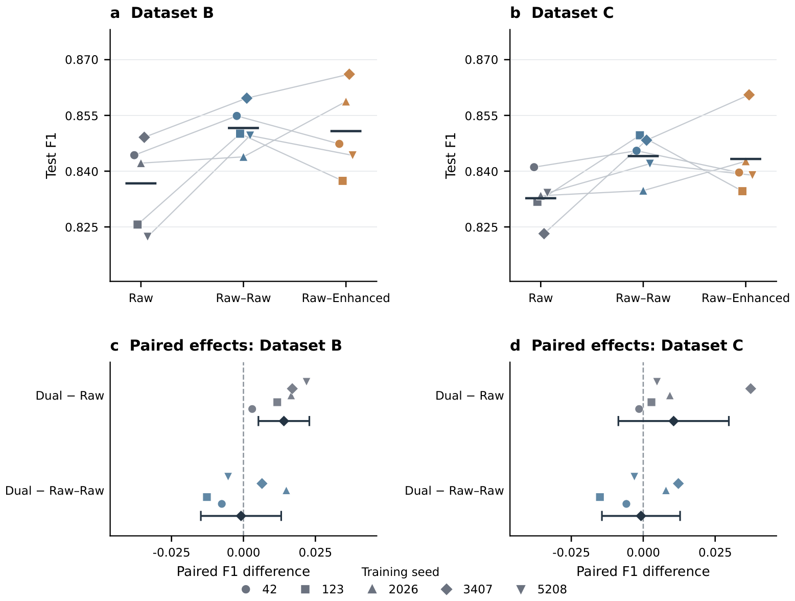
To further assess the reliability of the dual-view results across training initializations and to distinguish paired-view model capacity from the contribution of the Enhanced representation, Raw, equal-capacity Raw–Raw, and Raw–Enhanced were compared using the same five training seeds on Datasets B and C. As shown in Table 3, Raw–Enhanced improved the mean F1 score over Raw by 0.0141 on Dataset B, with positive differences for all five seeds. On Dataset C, the mean improvement was 0.0106, with positive differences for four of the five seeds. The dataset-level mean improvement was positive on both evaluation datasets, yielding an Across B–C mean F1 gain of 0.0123. The paired 95% confidence interval was entirely above zero on Dataset B, whereas the larger seed-to-seed variation on Dataset C produced an interval spanning zero.

Table 3. Paired F1 differences of Raw–Enhanced relative to Raw and the equal-capacity Raw–Raw control. Statistics within each dataset are computed from identical training seeds.

Unit	Contrast	n	Mean ± Sample SD	95% CI	Positive/Nonnegative Units
Dataset B seeds	Raw–Enhanced − Raw	5	$0.01405\pm 0.00713$	$[+0.00520,+0.02291]$	5/5
Dataset B seeds	Raw–Enhanced − Raw–Raw	5	$-0.00084\pm 0.01125$	$[-0.01481,+0.01313]$	2/5
Dataset C seeds	Raw–Enhanced − Raw	5	$0.01056\pm 0.01546$	$[-0.00864,+0.02976]$	4/5
Dataset C seeds	Raw–Enhanced − Raw–Raw	5	$-0.00078\pm 0.01094$	$[-0.01436,+0.01281]$	2/5
B–C dataset means	Raw–Enhanced − Raw	2	$0.01231\pm 0.00247$	$[-0.00989,+0.03451]$	2/2
B–C dataset means	Raw–Enhanced − Raw–Raw	2	$-0.00081\pm 0.00005$	$[-0.00122,-0.00039]$	0/2

Within each dataset, statistics are based on five paired training seeds ($n=5$). Across B–C, statistics are computed from the two paired dataset-level means ($n=2$).

The equal-capacity Raw–Raw comparison in Table 3 controls for the additional branch and model capacity because Raw–Raw and Raw–Enhanced use exactly the same dual-branch late-fusion architecture and differ only in the auxiliary input. Their F1 scores are numerically very similar, indicating that the F1 improvement over the single-channel Raw baseline cannot be attributed exclusively to the Enhanced representation. However, as shown in Table 2, Raw–Enhanced provides higher recall and lower conditional range and velocity RMSEs than Raw–Raw, suggesting that the Enhanced view mainly contributes complementary target-saliency and range–velocity localization information.

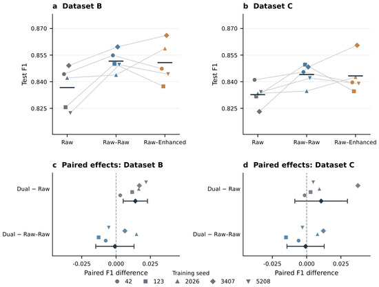
Figure 5 further visualizes the seed-level behavior on both evaluation datasets. The upper panels show the F1 scores of Raw, Raw–Raw, and Raw–Enhanced for all five training seeds, while the lower panels show the paired Raw–Enhanced-minus-Raw and Raw–Enhanced-minus-Raw–Raw differences. Raw–Enhanced exceeds Raw in all five paired runs on Dataset B and in four of the five runs on Dataset C, showing a consistent positive mean trend across the two independently generated simulation datasets despite the remaining training-seed variability.

Figure 5. Multi-seed F1 comparison and paired differences on simulation Datasets B and C. (a,b), F1 scores of Raw, Raw–Raw, and Raw–Enhanced for five training seeds; lines connect results obtained with the same seed. (c,d), Paired F1 differences of Raw–Enhanced relative to Raw and Raw–Raw; diamonds and whiskers indicate the mean and two-sided Student-t 95% confidence interval, respectively. The common confidence threshold of 0.45 was selected using Dataset A validation data and fixed before evaluation on Datasets B and C.The vertical dashed line at 0.000 represents the baseline of zero difference.

4.5. Computational Complexity and Runtime

As shown in Table 4, the Raw–Enhanced detector contains 10,793 trainable parameters and requires 27.33 MFLOPs, compared with 9334 parameters and 20.27 MFLOPs for Raw. With batch size one and FP32 inference, Raw–Enhanced requires 3.06 ms for a network forward pass on an NVIDIA RTX 4090 and 4.24 ms on one CPU thread. In comparison, the current CPU implementation of the median/MAD-based enhancement requires approximately $224.16\pm 14.42$ ms per frame, indicating that deterministic preprocessing rather than detector inference is the main computational bottleneck for end-to-end real-time operation.

Table 4. Model complexity and measured network-forward latency. Enhancement preprocessing is reported separately from detector inference.

Input	Parameters	FLOPs (M)	State (KiB)	CPU Forward (ms)	GPU Forward (ms)	Enhancement (ms)
Raw	9334	20.273	40.47	$2.9927\pm 0.2328$	$2.4360\pm 0.2291$	—
Raw–Raw	10,793	27.335	47.00	$4.2122\pm 0.1063$	$3.0615\pm 0.0584$	—
Raw–Enhanced	10,793	27.335	47.00	$4.2424\pm 0.0398$	$3.0625\pm 0.0699$	$224.16\pm 14.42$

5. Discussion and Conclusions

This study addresses the reduced target separability of FMCW radar RD representations under compound noise, clutter, and multipath by combining adaptive RD enhancement with a lightweight Raw–Enhanced dual-branch late-fusion detector. The proposed method first constructs an Enhanced saliency representation through local background estimation, robust MAD normalization, and adaptive zero-Doppler weighting. Raw and Enhanced features are then extracted by two independent shallow branches and fused at a later feature stage, allowing the original RD structure and locally enhanced target saliency to be exploited jointly.

Across two independently generated simulation datasets with five training seeds per dataset, the proposed Raw–Enhanced method increases the mean F1 score from 0.8347 to 0.8470 relative to the single-channel Raw baseline, corresponding to a relative improvement of 1.47%. Recall increases from 0.7470 to 0.7662, while the conditional range and velocity RMSEs over successfully matched detections decrease by 11.71% and 13.05%, respectively. The detector contains 10,793 trainable parameters, requires 27.33 MFLOPs, and has a measured network-forward time of approximately 3.06 ms on an RTX 4090. The current CPU implementation of the deterministic enhancement requires approximately 224 ms per frame, indicating that the end-to-end computational cost is dominated by the enhancement stage. Overall, the Raw–Enhanced framework improves detection completeness and range–velocity estimation under simulated compound interference while retaining a compact detection network. Future work will further evaluate the method using measured 77 GHz radar data and optimize the enhancement stage for real-time implementation.

References

- Waldschmidt, C.; Hasch, J.; Menzel, W. Automotive Radar—From First Efforts to Future Systems. IEEE J. Microwaves 2021, 1, 135–148. [Google Scholar] [CrossRef] [Scilit]
- Lin, J.J.; Li, Y.P.; Hsu, W.C.; Lee, T.S. Design of an FMCW Radar Baseband Signal Processing System for Automotive Application. SpringerPlus 2016, 5, 42. [Google Scholar] [CrossRef] [Scilit] [PubMed]
- Hyun, E.; Jin, Y.S.; Lee, J.H. A Pedestrian Detection Scheme Using a Coherent Phase Difference Method Based on 2D Range–Doppler FMCW Radar. Sensors 2016, 16, 124. [Google Scholar] [CrossRef] [Scilit] [PubMed]
- Zheng, Q.; Yang, L.; Xie, Y.; Li, J.; Hu, T.; Zhu, J.; Song, C.; Xu, Z. A Target Detection Scheme with Decreased Complexity and Enhanced Performance for Range–Doppler FMCW Radar. IEEE Trans. Instrum. Meas. 2021, 70, 1–13. [Google Scholar] [CrossRef] [Scilit]
- Chowdhury, D.; Melige, N.V.; Pal, B.; Gangopadhyay, A. Enhancing Outdoor Moving Target Detection: Integrating Classical DSP with mmWave FMCW Radars in Dynamic Environments. Electronics 2023, 12, 5030. [Google Scholar] [CrossRef] [Scilit]
- Xu, T.; Yu, D.; Du, L. A Bi-Objective Simulation Facility for Speed and Range Calibration of 24 GHz and 77 GHz Automotive Millimeter-Wave Radars for Environmental Perception. Electronics 2023, 12, 2947. [Google Scholar] [CrossRef] [Scilit]
- Yüksekkaya, F.; Franchi, N.; Lübke, M. On the Detection of Vulnerable Road Users—Simulating Limits of an FMCW Radar. Electronics 2024, 13, 2547. [Google Scholar] [CrossRef] [Scilit]
- Wang, X.; Ruan, Y.; Zhang, X. Effective Non-Stationary Clutter Suppression Method via Elevation Oblique Subspace Projection for Moving Targets Detection with a Space-Based Surveillance Radar. Electronics 2023, 12, 3110. [Google Scholar] [CrossRef] [Scilit]
- Li, Z.; Li, Y.; Wang, Y.; Zheng, T.; Qu, H. Millimeter-Wave Radar Clutter Suppression Based on Cycle-Consistency Generative Adversarial Network. Electronics 2024, 13, 4166. [Google Scholar] [CrossRef] [Scilit]
- Longman, O.; Villeval, S.; Bilik, I. Multipath Ghost Targets Mitigation in Automotive Environments. In Proceedings of the 2021 IEEE Radar Conference (RadarConf21), Atlanta, GA, USA, 7–14 May 2021; pp. 1–5. [Google Scholar] [CrossRef] [Scilit]
- Kraus, F.; Scheiner, N.; Ritter, W.; Dietmayer, K. The Radar Ghost Dataset—An Evaluation of Ghost Objects in Automotive Radar Data. In Proceedings of the 2021 IEEE/RSJ International Conference on Intelligent Robots and Systems (IROS), Prague, Czech Republic, 27 September–1 October 2021; pp. 8570–8577. [Google Scholar] [CrossRef] [Scilit]
- Zheng, L.; Long, J.; Lops, M.; Liu, F.; Hu, X.; Zhao, C. Detection of Ghost Targets for Automotive Radar in the Presence of Multipath. IEEE Trans. Signal Process. 2024, 72, 2204–2220. [Google Scholar] [CrossRef] [Scilit]
- Rohling, H. Radar CFAR Thresholding in Clutter and Multiple Target Situations. IEEE Trans. Aerosp. Electron. Syst. 1983, AES-19, 608–621. [Google Scholar] [CrossRef] [Scilit]
- Gandhi, P.P.; Kassam, S.A. Analysis of CFAR Processors in Nonhomogeneous Background. IEEE Trans. Aerosp. Electron. Syst. 1988, 24, 427–445. [Google Scholar] [CrossRef] [Scilit] [PubMed]
- Elias-Fuste, A.R.; de Mercado, M.G.G.; de los Reyes Davo, E. Analysis of Some Modified Ordered Statistic CFAR: OSGO and OSSO CFAR. IEEE Trans. Aerosp. Electron. Syst. 1990, 26, 197–202. [Google Scholar] [CrossRef] [Scilit]
- Kronauge, M.; Rohling, H. Fast Two-Dimensional CFAR Procedure. IEEE Trans. Aerosp. Electron. Syst. 2013, 49, 1817–1823. [Google Scholar] [CrossRef] [Scilit]
- Yan, B.; Roberts, I.P. Advancements in Millimeter-Wave Radar Technologies for Automotive Systems: A Signal Processing Perspective. Electronics 2025, 14, 1436. [Google Scholar] [CrossRef] [Scilit]
- Ślesicka, A.; Kawalec, A. Real-Time Hand Gesture Recognition for IoT Devices Using FMCW mmWave Radar and Continuous Wavelet Transform. Electronics 2026, 15, 250. [Google Scholar] [CrossRef] [Scilit]
- Wang, W.; Xu, H. RepHARNet: Human Activity Recognition Based on Radar Micro-Doppler Signatures Through Reparameterization. Electronics 2026, 15, 2729. [Google Scholar] [CrossRef] [Scilit]
- Zhang, L.; Tu, G.; Xu, Y.; Zhou, X. A Lightweight CNN-Based Method for Micro-Doppler Feature-Based UAV Detection and Classification. Electronics 2025, 14, 4831. [Google Scholar] [CrossRef] [Scilit]
- Zhang, A.; Nowruzi, F.E.; Laganiere, R. RADDet: Range-Azimuth-Doppler Based Radar Object Detection for Dynamic Road Users. In Proceedings of the 2021 18th Conference on Robots and Vision (CRV), Burnaby, BC, Canada, 26–28 May 2021; pp. 95–102. [Google Scholar] [CrossRef] [Scilit]
- Kim, W.; Cho, H.; Kim, J.; Kim, B.; Lee, S. YOLO-Based Simultaneous Target Detection and Classification in Automotive FMCW Radar Systems. Sensors 2020, 20, 2897. [Google Scholar] [CrossRef] [Scilit] [PubMed]
- Aydogdu, C.; Keskin, M.F.; Carvajal, G.K.; Eriksson, O.; Hellsten, H.; Herbertsson, H.; Nilsson, E.; Rydstrom, M.; Vanas, K.; Wymeersch, H. Radar Interference Mitigation for Automated Driving: Exploring Proactive Strategies. IEEE Signal Process. Mag. 2020, 37, 72–84. [Google Scholar] [CrossRef] [Scilit]
- Uysal, F. Phase-Coded FMCW Automotive Radar: System Design and Interference Mitigation. IEEE Trans. Veh. Technol. 2020, 69, 270–281. [Google Scholar] [CrossRef] [Scilit]
- Dai, J.; Du, L.; Sha, S.; Han, C.; Yao, Y. An Anti-Different Frequency Interference Algorithm for Environment-Aware Millimeter Wave Radar. Electronics 2023, 12, 3797. [Google Scholar] [CrossRef] [Scilit]
- Wang, J. CFAR-Based Interference Mitigation for FMCW Automotive Radar Systems. IEEE Trans. Intell. Transp. Syst. 2022, 23, 12229–12238. [Google Scholar] [CrossRef] [Scilit]
- Rameez, M.; Pettersson, M.I.; Dahl, M. Interference Compression and Mitigation for Automotive FMCW Radar Systems. IEEE Sens. J. 2022, 22, 19739–19749. [Google Scholar] [CrossRef] [Scilit]
- Howard, A.G.; Zhu, M.; Chen, B.; Kalenichenko, D.; Wang, W.; Weyand, T.; Andreetto, M.; Adam, H. MobileNets: Efficient Convolutional Neural Networks for Mobile Vision Applications. arXiv 2017, arXiv:cs.CV/1704.04861. [Google Scholar] [CrossRef] [Scilit]
- Sandler, M.; Howard, A.; Zhu, M.; Zhmoginov, A.; Chen, L.C. MobileNetV2: Inverted Residuals and Linear Bottlenecks. In Proceedings of the 2018 IEEE/CVF Conference on Computer Vision and Pattern Recognition, Salt Lake City, UT, USA, 18–23 June 2018; pp. 4510–4520. [Google Scholar] [CrossRef] [Scilit]
- Siddiq, K.; Hobden, M.K.; Pennock, S.R.; Watson, R.J. Phase Noise in FMCW Radar Systems. IEEE Trans. Aerosp. Electron. Syst. 2019, 55, 70–81. [Google Scholar] [CrossRef] [Scilit]
- Shen, W.; Wang, S.; Wang, Y.; Li, Y.; Lin, Y.; Zhou, Y.; Xu, X. Moving Target Detection Algorithm for Millimeter Wave Radar Based on Keystone-2DFFT. Electronics 2023, 12, 4776. [Google Scholar] [CrossRef] [Scilit]
- Richter, Y.; Balal, N. High-Resolution Millimeter-Wave Radar for Real-Time Detection and Characterization of High-Speed Objects with Rapid Acceleration Capabilities. Electronics 2024, 13, 1961. [Google Scholar] [CrossRef] [Scilit]
- Tian, F.; Wei, T.; Fu, W.; Wang, S. Research on Target Detection Algorithm for Complex Traffic Scenes Based on ADVI-CFAR. Electronics 2025, 14, 1474. [Google Scholar] [CrossRef] [Scilit]
- Zhou, L.; Wei, S.; Cui, Z.; Ding, W. YOLO-RD: A Lightweight Object Detection Network for Range–Doppler Radar Images. IOP Conf. Ser. Mater. Sci. Eng. 2019, 563, 042027. [Google Scholar] [CrossRef] [Scilit]
- Zhai, G.; Zhou, J.; Yang, H.; Zhang, Y. A Sea-Surface Radar Target-Detection Method Based on an Improved U-Net and Its FPGA Implementation. Electronics 2025, 14, 1944. [Google Scholar] [CrossRef] [Scilit]
- Liu, C.; Liu, S.; Zhang, C.; Huang, Y.; Wang, H. Multipath Propagation Analysis and Ghost Target Removal for FMCW Automotive Radars. IET Conf. Proc. 2021, 2020, 330–334. [Google Scholar] [CrossRef] [Scilit]
- Zhou, X.; Wang, D.; Krähenbühl, P. Objects as Points. arXiv 2019, arXiv:cs.CV/1904.07850. [Google Scholar] [CrossRef] [Scilit]
- Lin, T.Y.; Goyal, P.; Girshick, R.; He, K.; Dollár, P. Focal Loss for Dense Object Detection. In Proceedings of the 2017 IEEE International Conference on Computer Vision (ICCV), Venice, Italy, 22–29 October 2017; pp. 2980–2988. [Google Scholar] [CrossRef] [Scilit]
- Girshick, R. Fast R-CNN. In Proceedings of the 2015 IEEE International Conference on Computer Vision (ICCV), Santiago, Chile, 7–13 December 2015; pp. 1440–1448. [Google Scholar] [CrossRef] [Scilit]
- Kingma, D.P.; Ba, J. Adam: A Method for Stochastic Optimization. arXiv 2015, arXiv:cs.LG/1412.6980. [Google Scholar] [CrossRef] [Scilit]
Disclaimer/Publisher’s Note: The statements, opinions and data contained in all publications are solely those of the individual author(s) and contributor(s) and not of MDPI and/or the editor(s). MDPI and/or the editor(s) disclaim responsibility for any injury to people or property resulting from any ideas, methods, instructions or products referred to in the content. |
© 2026 by the authors. Licensee MDPI, Basel, Switzerland. This article is an open access article distributed under the terms and conditions of the Creative Commons Attribution (CC BY) license.