


Abstract
Turboshaft engine bladed disks are prone to typical faults such as tenon-root cracks and rub-impact during operation. Blade tip timing (BTT) signals inherently contain both blade arrival-time information and blade spatial-distribution information, which are coupled with each other. Conventional data representation methods lack the capability to deeply mine such complex coupling relationships. To address this issue, a diagnostic method integrating a physically coupled multi-channel two-dimensional spatiotemporal representation with an attention-enhanced residual network is proposed. First, the Error Compensation Coefficient (ECC) method is employed to correct the raw blade spacing data, eliminating static deviations introduced by manufacturing and assembly. Second, the corrected data are organized into a two-dimensional field indexed by blade spacing and revolution—the physical variables of the measurement—and three physically complementary channels are constructed, namely the ECC baseline value, the first-order temporal difference (ΔS) and the spatial coefficient of variation (SCV), forming an ECC–ΔS–SCV three-channel two-dimensional spatiotemporal feature map that represents the magnitude, the temporal dynamics and the spatial cooperativity of the blade group, respectively. Finally, the feature map is decoded by a deliberately standard ResNet18 backbone embedded with the Convolutional Block Attention Module (CBAM, with stage-adapted spatial kernels), so that the contribution of the representation can be isolated from that of the network. Experimental data were collected from a self-built mortise–tenon bladed-disk test rig under three conditions—healthy, tenon-root crack and rub-impact—at rotational speeds of 500, 1000 and 1500 rpm. Each configuration is trained ten times using a fixed data split with different random seeds, and all results are reported as mean ± standard deviation. Under identical data splits and training configurations, the proposed method achieves mean classification accuracies of 95.07%, 92.62% and 91.25% at the three speeds (92.98% on average), outperforming five mainstream deep learning benchmark models. Ablation studies confirm that each feature channel is necessary and the attention module as a whole is beneficial, and that the improvement is attributable to the representation rather than to model scale; a leave-one-speed-out evaluation further quantifies the performance degradation when the test speed is excluded from training. This study provides a physically coupled representation and an effective diagnostic framework for BTT-based fault diagnosis of rotating machinery.
1. Introduction
Turboshaft engine disks operate under prolonged high-temperature, high-pressure and high-speed conditions, making them susceptible to fatigue crack initiation and subsequent rub-impact, which can lead to deterioration of dynamic balance and even catastrophic flight accidents [1,2]. Blade-root fatigue cracking and blade–casing rub-impact are among the most frequently reported structural failures of aero-engines [1], and the condition monitoring and remaining-life prediction of engine rotating components have consequently become an active research field [3]. This underscores the critical importance of blade-disk system fault diagnosis for flight safety. Blade tip timing (BTT) technology, by virtue of its non-contact nature and capacity for simultaneous multi-blade measurement, has become a key monitoring technique for blade-disk condition assessment [4,5,6]. At present, BTT-based blade vibration monitoring and rotor system fault diagnosis have found extensive application in typical scenarios such as mistuning analysis [7], crack identification, and rub-impact monitoring.
In the domain of crack identification, existing methods principally follow two technical routes. The first route employs blade natural frequency or resonance characteristics as diagnostic indicators. Witoś [8] demonstrated that morphological changes in resonance features can be used to determine the presence of cracks. Zielinski et al. [9] adopted the peak dynamic stress of the blade’s second bending mode at resonance as a sensitive indicator, successfully identifying high-cycle fatigue cracks induced by high-order resonance. Xu et al. [10] exploited the drift of natural frequency caused by cracks and employed synchroextracting transform to extract time-frequency features for crack propagation monitoring. Guo et al. [11] systematically analyzed the effects of crack position and length on the natural frequency, modal localization parameters, resonance frequency region, and vibration response localization of blade-disk systems. All of the above methods presuppose a high-precision rotational speed reference and rely on a key-phasor sensor for accurate frequency extraction. The second route constructs multi-dimensional feature spaces through data-driven or model-fusion approaches. Chen et al. [12] extracted nine-dimensional features from BTT data and combined them with principal component analysis to achieve crack identification. Du et al. [13] proposed a hybrid model-and-data-driven strategy, employing Bayesian linear regression to jointly cluster amplitude and frequency for crack discrimination. These methods broaden the feature dimension, but the features are still extracted from vibration parameters synchronized by a key-phasor signal; when the speed reference is absent, the feature space becomes difficult to construct.
Notably, Wu et al. [14] introduced blade spacing into the field of crack diagnosis, jointly adopting frequency and blade spacing as diagnostic indicators. They used the Lomb–Scargle periodogram to determine the presence of cracks and subsequently located the faulty blade by means of blade frequency and inter-blade spacing. This work extended the utilization dimension of BTT signals—from vibration-based parameters alone to geometric-type parameters—but its frequency identification stage still depends on a key-phasor sensor to provide the rotational speed reference. Building on this, Guo et al. [15] further extended the blade-spacing approach to the detection of cracks at the bottom of the disk mortise slots. Through finite-element stress analysis and crack propagation path simulation, they revealed the pattern whereby a mortise crack causes the blade spacing on one side of the crack to increase and that on the other side to decrease, and they established a diagnostic procedure that uses the standard deviation of blade spacing to determine the presence of cracks and the measurable amplitude of blade spacing to distinguish crack types. This work calculates blade spacing from the arrival time difference between adjacent blades, thereby freeing itself from key-phasor dependence. However, it treats the static system errors arising from manufacturing and assembly merely by subtracting the baseline value obtained in the healthy state, without establishing a systematic error compensation mechanism. Consequently, the diagnostic potential of the blade-spacing signal remains insufficiently exploited.
In the domain of rub-impact fault diagnosis, existing studies have primarily focused on capturing the impact response or torsional vibration changes induced by rub-impact. Wang Weimin et al. [16] achieved fault early warning by monitoring rotor torsional vibration and proposed a correction method that addresses both manufacturing/assembly deviations and blade-vibration-induced spacing non-uniformity. Wu Shuming et al. [17] and Wu et al. [18] respectively combined enhanced sparse decomposition and digital twin methods to extract rub-impact features. These methods likewise rely on a key-phasor sensor for synchronous vibration averaging or torsional vibration calculation, and the rub-impact signature is tightly coupled in the time and space domains—blade vibration, torsional vibration, and assembly deviations jointly modulate the blade arrival time. When the key-phasor signal is absent or the error compensation lacks systematic rigor, the contributions of individual factors become intertwined and difficult to disentangle.
In summary, although existing studies have validated the sensitivity of BTT signals to blade-disk faults, two common bottlenecks persist. First, the majority of diagnostic procedures are heavily reliant on a key-phasor sensor, yet the confined internal space and demanding installation conditions of aero-engines often render the key-phasor signal unobtainable in real service environments. Second, the decoupling and representation of the time-domain and space-domain information coupled within BTT signals remain inadequate. Even though Guo et al. [15] have realized key-phasor-free blade-spacing calculation, the elimination of static system errors such as those from manufacturing and assembly still lacks systematic rigor, and an effective framework for representing multi-source coupled features—including blade vibration and rub-impact—is likewise absent.
To address these issues, this paper develops a blade-disk fault diagnosis method that takes blade spacing as the core diagnostic parameter and does not rely on a key-phasor sensor. The focus of the paper is the representation of BTT signals for diagnosis, not the design of the network; the network is kept standard so that the effect of the network can be separated from that of the representation. The main contributions are as follows. (1) An Error Compensation Coefficient (ECC) method is introduced, which establishes a compensation coefficient for each blade spacing from healthy-state data and removes the static errors introduced by manufacturing and assembly. (2) An ECC–ΔS–SCV multi-channel two-dimensional spatio-temporal representation is constructed. The corrected data are arranged as a two-dimensional map whose rows are the revolutions and whose columns are the blade spacings, and three complementary channels are generated to describe the absolute magnitude (ECC baseline), the temporal variation (first-order time difference) and the spatial cooperativity (spatial coefficient of variation) of the blade group; each channel is linked to a fault mechanism, and the ablation experiments show that each is needed. (3) A standard attention-enhanced residual network (CBAM-ResNet-18) is adopted for classification; channel attention adjusts the weight of the three channels while spatial attention marks the sensitive regions on the spacing–revolution grid, and the choice is supported by comparisons with five alternative backbones and by the branch-wise ablations. The effectiveness of the proposed method is validated using BTT signals acquired from a self-built tenon-jointed blade-disk test rig at rotational speeds of 500, 1000 and 1500 rpm.
2. Experimental Data Acquisition and Preprocessing
2.1. Blade Tip Timing Principle and Blade Spacing Calculation
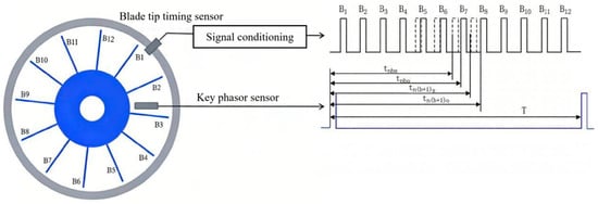
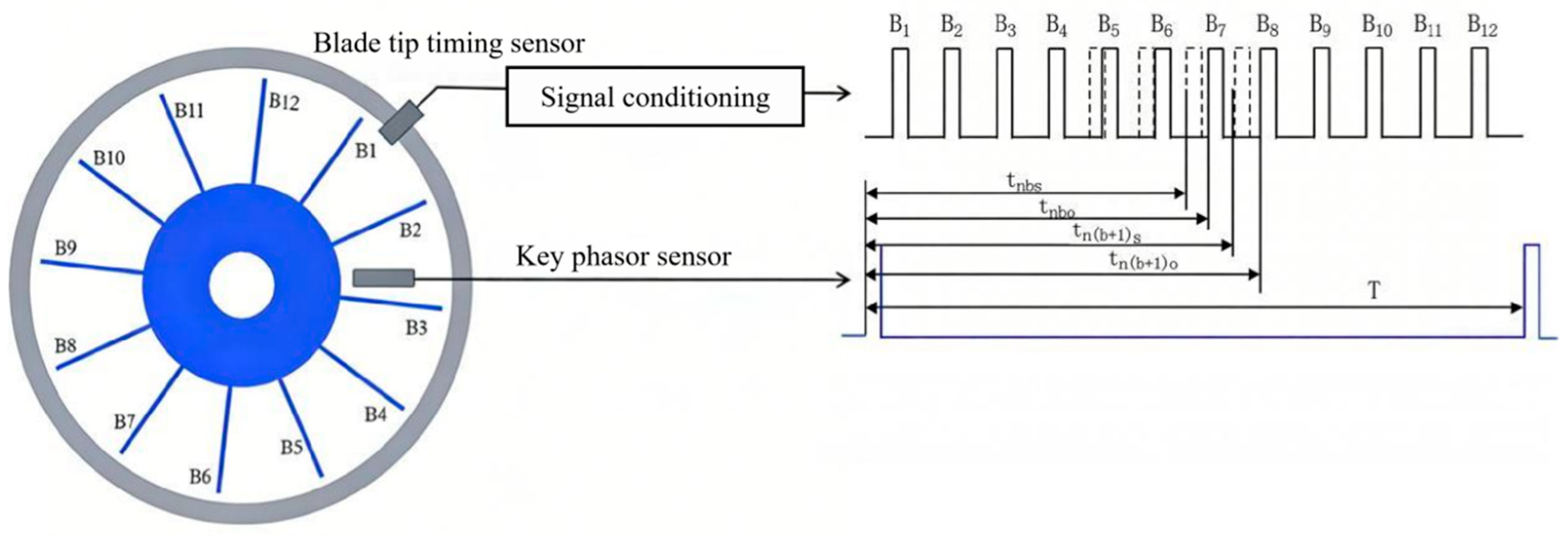
The basic principle of blade tip timing (BTT) technology is illustrated in Figure 1. A BTT sensor is mounted on the casing and generates a pulse each time a blade tip sweeps past, thereby capturing the blade’s arrival time. A synchronously arranged key-phasor sensor outputs once-per-revolution reference pulses. If a blade undergoes vibration, its arrival time at the BTT sensor will be correspondingly advanced or delayed. By processing the acquired time series, the vibration information of all blades can be extracted, enabling real-time monitoring of the bladed disk’s operating condition [19].
Figure 1.
Basic principle of the blade tip timing method.
The key aspect of conventional BTT technology lies in using multiple sensors to measure and reconstruct the absolute vibration displacement of individual blades [20]. However, this study focuses on a parameter with greater engineering practicality: blade spacing. Blade spacing measurement retains the advantages of BTT technology—namely, its non-contact nature and high responsiveness—while circumventing the stringent requirements for sensor layout and reconstruction algorithms associated with blade vibration displacement measurement, and is more sensitive to coordination-related faults in the bladed disk system.
In Figure 1, where tnbo is the theoretical arrival time of blade b in the absence of vibration, and tn(b+1)o is that of blade (b + 1). The spacing between blade b and blade (b + 1) is then given by:
where is the theoretical spacing between blade b and blade (b + 1) at rotational speed ω, r is the distance from the blade tip to the center of the blade disk, and ω is the rotational speed of the blade disk.
Where tnbs is the actual arrival time of blade b, and tn(b+1)s is that of blade (b + 1). The spacing between blade b and blade (b + 1) is then given by:
where is the actual spacing between blade b and blade b + 1 at rotational speed ω.
2.2. Experimental Platform and Fault Simulation
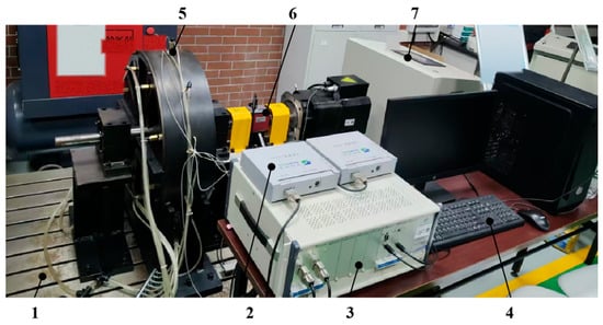
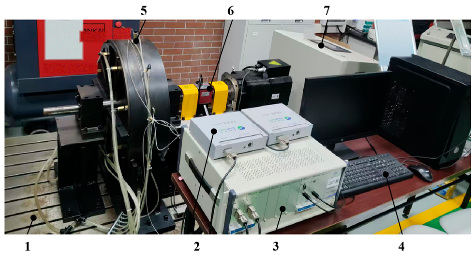
To acquire the dynamic response data of the blade disk under different health states, a tenon-connected blade disk fault simulation experimental platform was designed and constructed, as shown in Figure 2. The platform consists of four parts: (1) the tenon-connected blade disk test rig, comprising a single-stage tenon-connected blade disk and a drive motor; (2) the BTT signal acquisition system, consisting of fiber-optic BTT sensors, preamplifiers, and a high-speed data acquisition chassis with a sampling rate of 100 MHz; (3) the test rig control system for speed regulation—500 rpm, 1000 rpm, and 1500 rpm were adopted in this experiment; and (4) a data acquisition and analysis computer for real-time monitoring and data storage.
Figure 2.
Overall view of the blade tip timing experimental platform. 1. Platform base plate; 2. Preamplifier; 3. Blade vibration data acquisition chassis; 4. Computer; 5. Blade tip timing sensor; 6. Tenon-connected blade disk test platform; 7. Test rig control system.
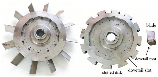
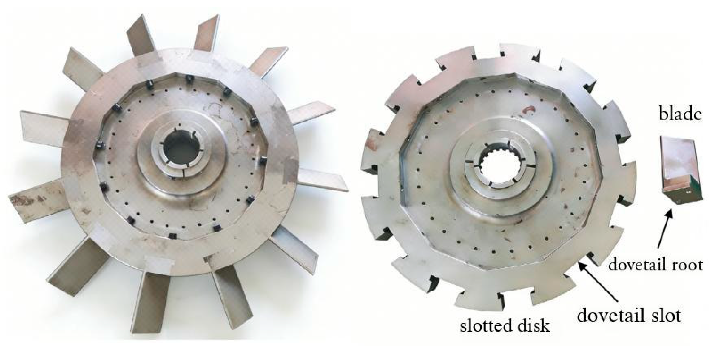
The tenon-connected blade disk used in the experiment is shown in Figure 3. It consists of a slotted disk and 12 blades, with the main body made of 45# steel. Each blade is 82 mm in length, and the disk has a radius of 200 mm. The blade installation angle was set to 45°.
Figure 3.
Physical view of the bladed disk.
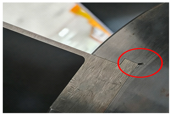
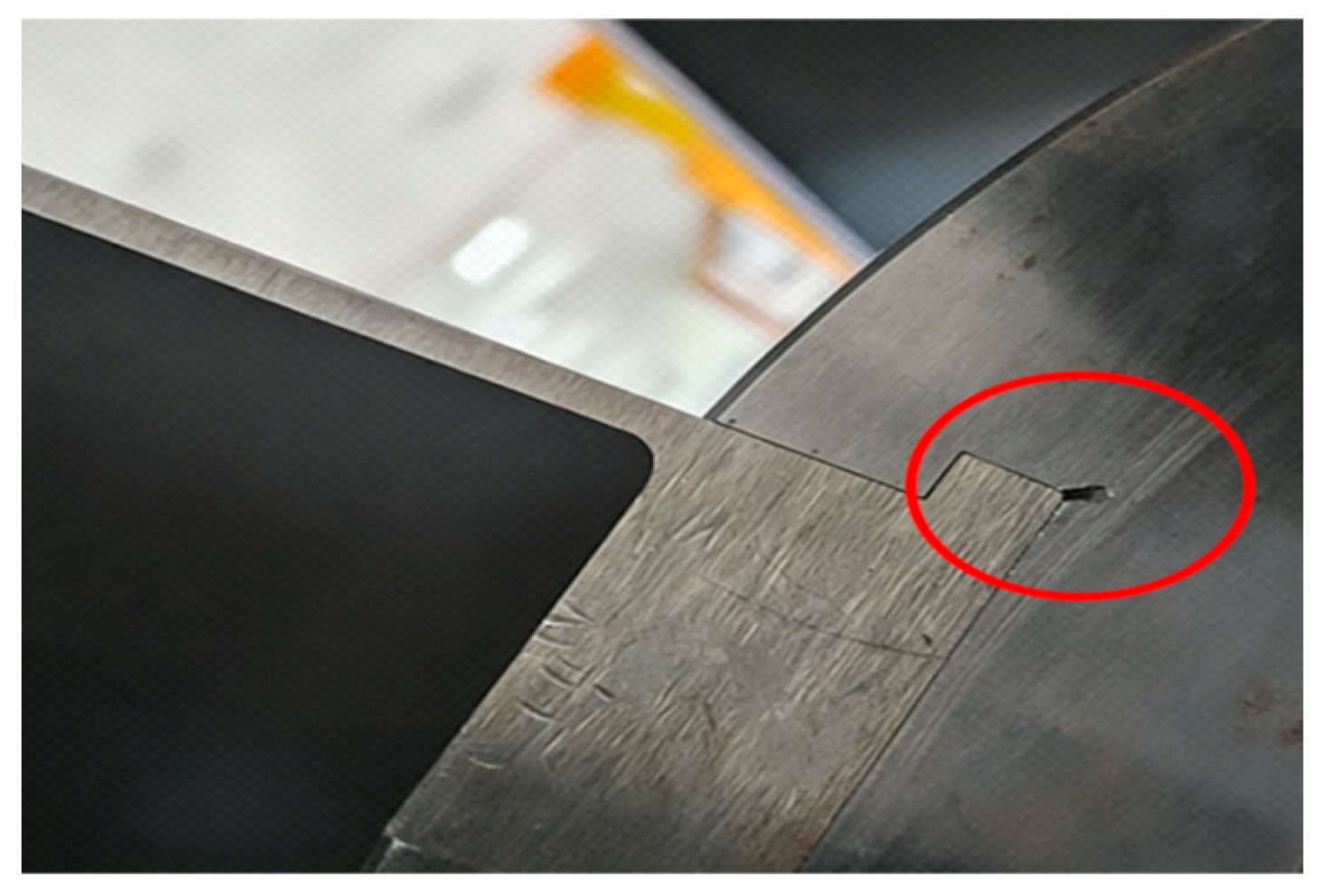
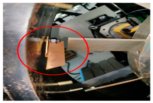
Tenon-root crack fault simulation. Under centrifugal loading, significant stress concentration exists at the bottom of the tenon groove, making it a sensitive area for fatigue crack initiation. A 3 mm long crack was prefabricated at the bottom of the tenon groove of blade No. 7, as shown in Figure 4.
Figure 4.
Physical photograph of the bladed disk with a tenon crack. The red circle indicates the crack.
Data acquisition. Under both the healthy and cracked conditions, BTT data were continuously collected for 750 rotation cycles at each of the three rotational speeds, with 12 blade spacing values per cycle.
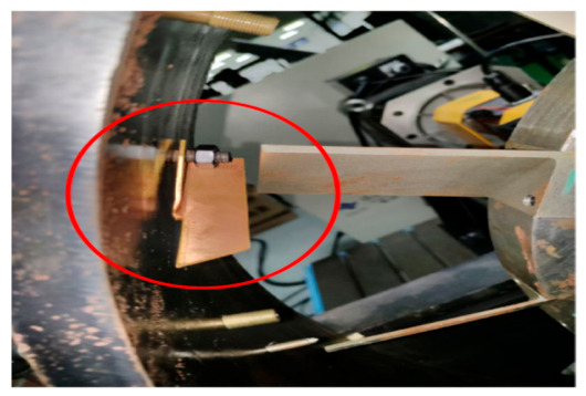
Rub-impact fault simulation. The rub-impact device is shown in Figure 5. A copper rubbing element is fixed to the inner side of the casing by bolts, and the radial clearance between the rubbing element and the blade tip can be adjusted via a regulating nut, thereby achieving stable rub-impact excitation. After ensuring that the rubbing element would make contact with each blade, rub-impact condition data were collected for 750 cycles at each of the three rotational speeds.
Figure 5.
Rubbing device. The red circle indicates the copper rubbing element fixed to the inner side of the casing.
In summary, data were collected for 750 cycles at each rotational speed under three conditions—healthy, cracked, and rub-impact—with each sample consisting of 12 blade spacing measurements within a single cycle.
2.3. ECC-Based Data Preprocessing
Static geometric errors introduced during blade machining and assembly are directly reflected in the baseline offset of each blade spacing. These errors are superimposed on and coupled with the dynamic spacing fluctuations caused by vibration in the measured data, and their amplitude may be on the same order of magnitude as early-stage weak fault signals, severely interfering with subsequent diagnosis. To address this issue, this section introduces the error compensation coefficient (ECC) method to correct the raw data.
The core idea of ECC is as follows: under healthy conditions, the blade spacings of a symmetric blade disk should theoretically be consistent, and the discrepancies in actual measurements primarily originate from static system deviations. Using the healthy-state data as a reference, compensation coefficients are established for each blade spacing, and the raw measurements are uniformly mapped to the same reference baseline. After removing the static errors, the variation components in the corrected data predominantly reflect the true dynamic spacing fluctuations.
Consider a blade disk rotor with a total of N blades, and T = 750 stable rotation cycles of data (the complete healthy record of Section 2.2) collected under healthy conditions:
Healthy baseline data acquisition. Under healthy conditions where the blade disk is confirmed to be fault-free, blade spacing data are collected during steady operation at the target rotational speed for T stable rotation cycles, serving as the healthy baseline dataset for ECC calculation, denoted as Sbase. The coefficients are computed from the healthy-state record alone. That record contains no cracked or rub-impact data, and a single set of per-blade constants is applied to every operating condition, so the coefficients carry no class information and cannot leak the label of any evaluation window.
The mean value of each blade spacing is calculated as :
where is the spacing value between blade i and blade i + 1 in the t-th rotation cycle of the healthy baseline dataset Sbase.
Establish a global reference baseline. The overall mean of the mean blade spacings across all N blades is calculated as .
Calculate the error compensation coefficients. For each blade spacing, its error compensation coefficient ECCi is defined as the ratio of the global reference baseline to its static mean spacing:
Correct the data. The raw data under any operating condition are corrected as follows:
where is the corrected value.
After correction, each blade spacing is uniformly calibrated to the global reference baseline, eliminating the inherent deviations caused by static errors. As a result, the dynamic spacing variations induced by faults become more clearly distinguishable, providing input data with a high signal-to-noise ratio (SNR) for subsequent feature extraction.
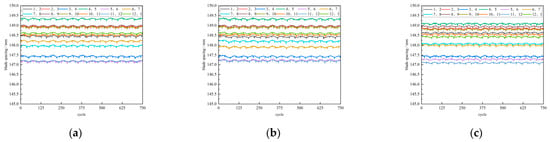
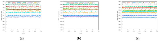
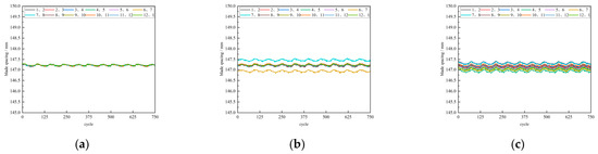
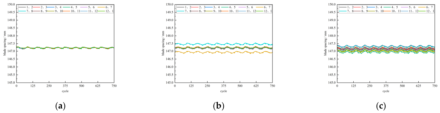
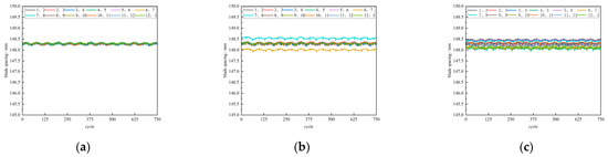
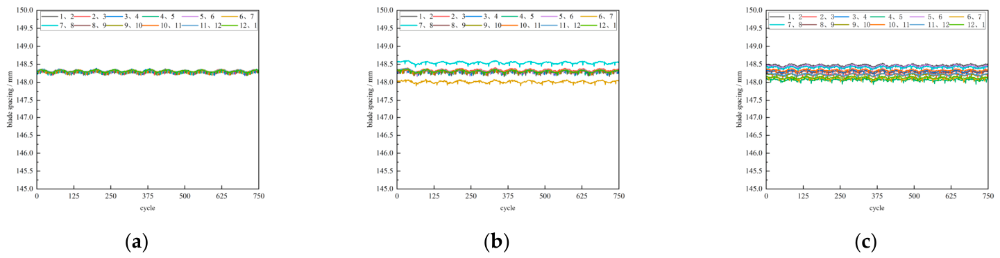
Through the correction process, a measured BTT dataset for blade disk fault diagnosis research was successfully constructed. Figure 6, Figure 7 and Figure 8 show the variation curves of adjacent blade spacings with rotation cycles for each health state at the three rotational speeds before error correction. It can be observed that, dominated by static system errors, the curves of the healthy, cracked, and rub-impact conditions lack clear separation boundaries, making different fault modes difficult to distinguish.
Figure 6.
Variation in adjacent blade tip spacing with number of revolutions for different bladed disk conditions before error correction at 500 rpm. (a) Healthy; (b) Crack; (c) Rub. Legend numbers denote adjacent blade pairs (1–2, 2–3, …, 12–1).
Figure 7.
Variation in adjacent blade tip spacing with number of revolutions for different bladed disk conditions before error correction at 1000 rpm. (a) Healthy; (b) Crack; (c) Rub. Legend numbers denote adjacent blade pairs (1–2, 2–3, …, 12–1).
Figure 8.
Variation in adjacent blade tip spacing with number of revolutions for different bladed disk conditions before error correction at 1500 rpm. (a) Healthy; (b) Crack; (c) Rub. Legend numbers denote adjacent blade pairs (1–2, 2–3, …, 12–1).
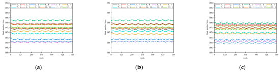
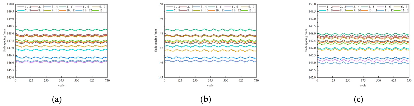
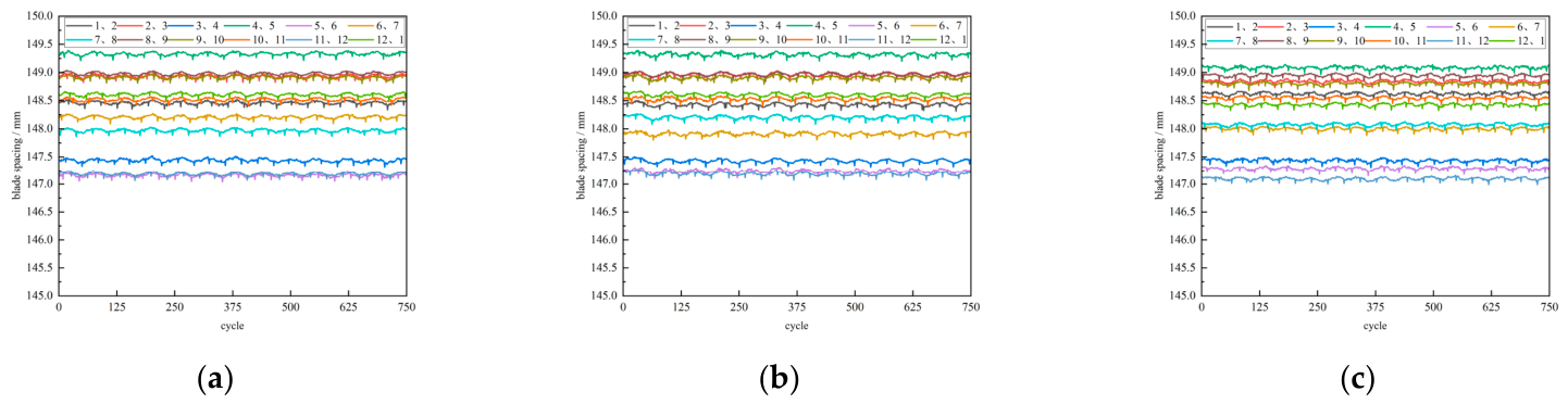
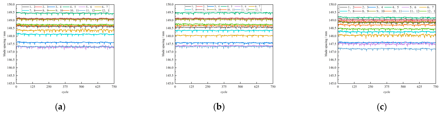
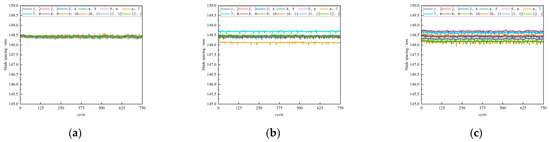
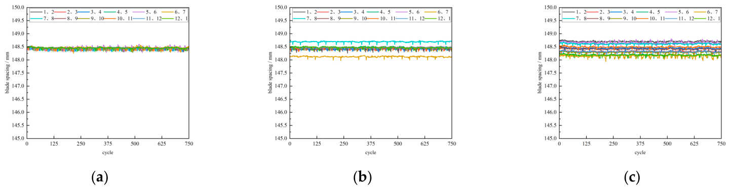
Figure 9, Figure 10 and Figure 11 show the corresponding curves after error correction at the three rotational speeds. Under the healthy condition, the adjacent blade spacing curves almost completely overlap, with negligible amplitudes, indicating that the ECC correction removes the stratified discrepancies caused by machining and assembly errors, and the system exhibits highly uniform dynamic response. Under the cracked condition, most blade spacing curves remain overlapped and stable; only the spacings 6–7 and 7–8, which are associated with the tenon-root crack of blade No. 7, exhibit localized baseline offset and slight fluctuations, precisely highlighting the local effect of the crack. Under the rub-impact condition, the blade spacing curves no longer overlap stably but instead display pronounced dispersion and global vibration disturbance, forming a sharp contrast with the uniformity of the healthy condition and the localized anomaly of the cracked condition. In summary, after ECC correction, the three health states exhibit markedly different distribution characteristics in the time-domain curves, providing a distinguishable data foundation for subsequent fault mode identification.
Figure 9.
Variation in adjacent blade tip spacing with number of revolutions for different bladed disk conditions after error correction at 500 rpm. (a) Healthy; (b) Crack; (c) Rub. Legend numbers denote adjacent blade pairs (1–2, 2–3, …, 12–1).
Figure 10.
Variation in adjacent blade tip spacing with number of revolutions for different bladed disk conditions after error correction at 1000 rpm. (a) Healthy; (b) Crack; (c) Rub. Legend numbers denote adjacent blade pairs (1–2, 2–3, …, 12–1).
Figure 11.
Variation in adjacent blade tip spacing with number of revolutions for different bladed disk conditions after error correction at 1500 rpm. (a) Healthy; (b) Crack; (c) Rub. Legend numbers denote adjacent blade pairs (1–2, 2–3, …, 12–1).
The above ECC correction results demonstrate that the corrected data exhibit a high degree of baseline consistency, static system errors are effectively suppressed, the fluctuation characteristics induced by faults become more distinct, and the blade spacing variation components caused by cracks and rub-impact are significantly enhanced. Data correction is therefore of great significance for the effectiveness and engineering practicality of the subsequent intelligent diagnostic pipeline.
However, Figure 9, Figure 10 and Figure 11 reveal a critical difficulty: the spacing deviations of adjacent blade pairs 6–7 and 7–8 caused by cracks are very small, comparable in magnitude to the random fluctuations inherent in the blade spacing of individual blades under healthy conditions. Based solely on single-revolution spacing values, it is difficult to determine whether a slight deviation originates from a crack-induced change or merely from incidental measurement fluctuations. Meanwhile, the degree of dispersion among individual blade spacings increases markedly under rub-impact conditions, yet this manifests in the visualization of the T × N blade spacing data only as curve divergence, lacking a per-revolution scalar metric for quantification.
3. Multi-Channel Two-Dimensional Spatio-Temporal Representation and Diagnostic Model
3.1. ECC–ΔS–SCV Spatio-Temporal Representation
Section 2.3 obtained the corrected T × N blade spacing data using the ECC method. As noted above, these data do not explicitly express the per-revolution variation or intra-revolution dispersion of blade spacing. To this end, this section introduces the first-order temporal difference ΔS as the second channel, which extracts the spacing variation between adjacent revolutions and reflects the dynamic change trend and instantaneous impulses of the signal. The spatial coefficient of variation SCV is introduced as the third channel to quantify the dispersion degree of individual blade spacings on a per-revolution basis. Together with the ECC-corrected spacing, these three components form a T × N × 3 three-channel two-dimensional spatio-temporal feature map.
Channel 1: error-compensated baseline value (ECC). The preprocessed blade spacing data are directly used, providing an absolute magnitude reference.
Channel 2: first-order temporal difference (ΔS). The variation between adjacent rotation cycles for the same blade spacing is computed to capture instantaneous impulses and gradual trends.
Set to zero when t = 1.
Channel 3: spatial coefficient of variation To characterize the disruption of blade spatial cooperativity caused by faults, the mean μt and standard deviation σt of all N blade spacings are calculated for the t-th cycle:
The spatial coefficient of variation is defined as the ratio of the standard deviation to the mean:
This scalar value is assigned to all blade positions in the t-th cycle, forming a spatially uniform yet temporally varying feature layer:
X(3)(t,i) = SCVt, ∀i ∈ [1,N].
Because the same scalar is replicated across all twelve blade positions, Channel 3 quantifies the dispersion of the blade group as a whole and, by construction, does not retain the location of the anomalous blade. The spatial location of a fault is instead carried by Channels 1 and 2, whose entries are indexed by blade spacing. Channel 3 should therefore be read as a per-revolution measure of the loss of blade-set coordination rather than as a spatially resolved feature.
The physical meanings of the three channels are summarized in Table 1.
Table 1.
Physical meanings of the ECC-ΔS-SCV map multi-channel features.
To eliminate dimensional differences, min–max normalization is applied to each channel independently:
For the c-th channel of any sample, the following transformation is applied:
where and are the global maximum and minimum values of the c-th channel over the training set.
After normalization, the resulting three-channel two-dimensional spatio-temporal feature map serves as the input to the subsequent deep convolutional neural network.
Both axes of the map are measurement variables: a row corresponds to a revolution and a column to a blade spacing, so neighboring entries are physically related. This differs from image-like inputs constructed from a time series, such as time–frequency maps, whose coordinates are transform parameters. Deep networks have also been applied to mechanical signals in other structural-health-monitoring domains—for example, deep residual networks trained on time–frequency images for acoustic-emission source localisation [21] and compact one-dimensional CNNs applied to raw structural responses for damage detection [22]. Those studies, however, address different sensing mechanisms and structures; the present work instead arranges the BTT signals so that both axes of the input are the physical measurement variables of the diagnosed component. The channels also respond to the two faults in different ways: a tenon-root crack leaves a persistent offset at the cracked blade, whereas rub-impact produces intermittent impulses and weakens the spatial consistency of the blade set. Section 4.5 reports the loss of accuracy when each channel is removed in turn.
3.2. CBAM-ResNet18 Diagnostic Model and Overall Pipeline
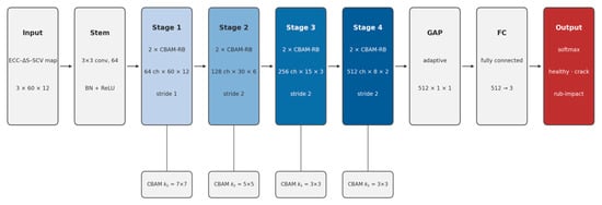
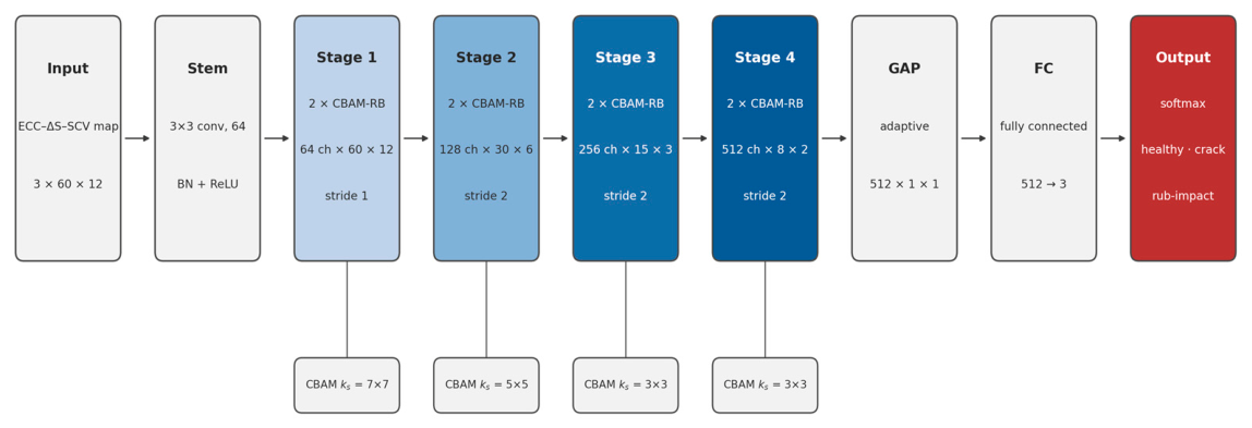
The ECC–ΔS–SCV map has a size of 60 × 12 × 3, with information distributed across the temporal, spatial, and multi-channel dimensions. In this paper, ResNet18 [23] is adopted as the backbone network: its 18-layer depth is sufficient for extracting hierarchical spatiotemporal features while being resistant to overfitting, and the residual connections facilitate gradient propagation and weak fault capture. On this basis, a CBAM module [24] is embedded after the convolutional layer and before the shortcut connection in each residual block, enabling sequential recalibration of key features through channel and spatial attention. To accommodate the decreasing spatial sizes across the residual stages, the spatial attention employs stage-adapted convolution kernel sizes—7 × 7, 5 × 5, 3 × 3 and 3 × 3 for the four stages—rather than the fixed 7 × 7 kernel of the original CBAM. The overall network architecture is as follows: the ECC–ΔS–SCV map is input → an initial convolution → four CBAM residual stages → global average pooling → a fully connected layer that outputs the probabilities of the three classes (healthy, crack, and rub-impact), as illustrated in Figure 12.
Figure 12.
CBAM-ResNet18 network architecture.
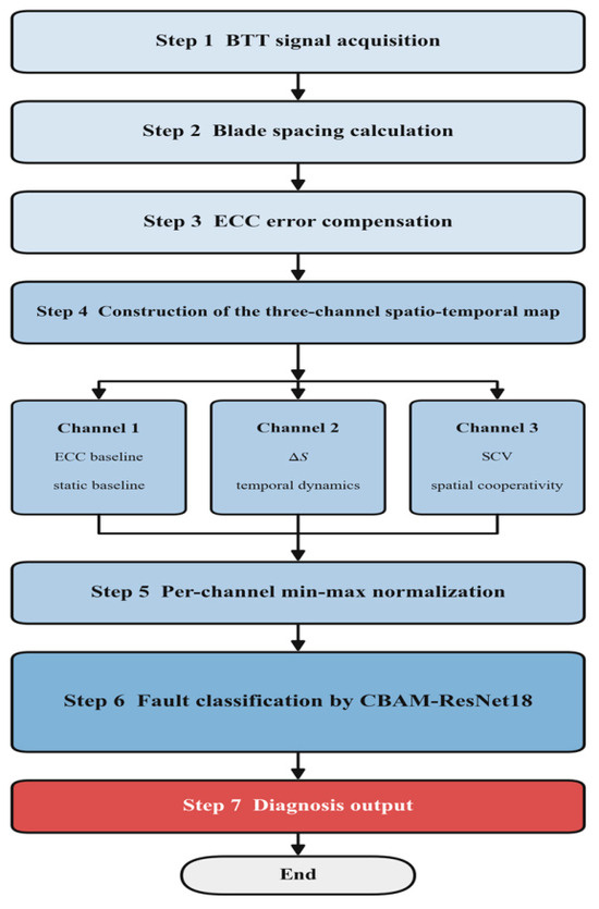
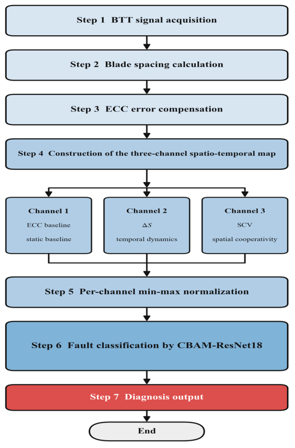
Model training adopts the cross-entropy loss function and the Adam optimizer, combined with a cosine annealing learning rate schedule. The complete diagnostic pipeline is shown in Figure 13: the ECC-corrected BTT data undergo three-channel spatiotemporal map construction and are then fed into CBAM-ResNet18 for feature extraction and classification.
Figure 13.
Overall flow of the fault diagnosis.
The backbone is kept standard so that the effect of the representation can be assessed separately from that of the network. CBAM matches the structure of the map: channel attention adjusts the weight of the three channels, while spatial attention acts on the spacing–revolution grid. Under the same training protocol, using both branches is better than using channel attention alone (SE-ResNet-18, Section 4.4), and Section 4.5 gives the loss of accuracy when either branch is retained alone.
4. Experimental Validation and Result Analysis
4.1. Dataset Construction and Model Configuration
- (1)
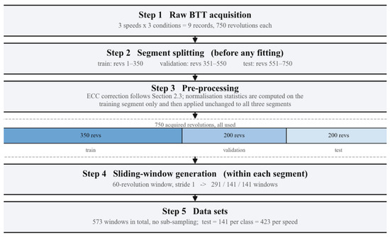
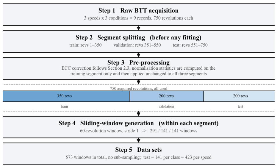
- To fully exploit the temporal information and generate sufficient training samples, a sliding-window procedure is adopted. Each of the nine records comprises 750 consecutive revolutions and is partitioned by acquisition segment before any window is generated: revolutions 1–350 form the training segment, revolutions 351–550 the validation segment, and revolutions 551–750 the test segment. Revolutions are delimited without a once-per-revolution reference: the first spacing sample of the record is taken as the blade 1–2 spacing, and every twelve successive samples—one complete passage of the twelve blades—constitute one revolution, so that both the revolution boundaries and the blade indices follow from the acquisition order and the known blade count. The normalization statistics are computed on the training segment only and then applied unchanged to the validation and test segments. All preprocessing steps other than the ECC calibration are therefore fitted on the training segment alone. The ECCs are a per-blade static calibration obtained from the healthy-state record and applied unchanged to every class and every split; because that record contains no cracked or rub-impact data, the coefficients carry no class information. Sliding windows of 60 consecutive revolutions with a stride of 1 are then generated within each segment only, so that no window crosses a segment boundary. For the data within each window, the procedure described in Section 3.1 is applied independently to construct an ECC–ΔS–SCV map (a three-channel two-dimensional spatio-temporal feature map) of size 60 × 12 × 3. A speed–condition combination therefore yields 291, 141 and 141 windows for the training, validation and test sets, respectively—573 in total, approximately 50%/25%/25%—with the healthy, crack and rub-impact classes labeled 0, 1 and 2. The same partition is applied identically to all nine records, giving 873/423/423 windows per rotational speed and 2619/1269/1269 in total (Figure 14, Table 2). Because the three segments are mutually disjoint and windows never cross a segment boundary, no test window shares a single revolution with any training window; the only information shared with the test side is the healthy-class ECC calibration described above. The validation set is used solely for monitoring convergence and for the window-length sensitivity study in Section 4.3; the test set is reserved for the final evaluation only.Figure 14. Data flow from raw BTT acquisition to the training, validation and test sets.Table 2. Number of samples for each combination of rotational speed, fault condition and data subset.
- (2)
- Model configuration. The classification model adopts the CBAM-ResNet-18 architecture constructed in Section 3.2, with cross-entropy as the loss function and Adam as the optimizer [25]. To counter over-parameterisation, a weight decay of 1 × 10⁻⁴ is applied. The initial learning rate is set to 0.001 and is dynamically adjusted using a cosine annealing schedule whose period must be specified in advance [26]. During training, the batch size is 32 and the number of training epochs is 50; both are fixed before training, and because a cosine schedule requires the total number of epochs to be known a priori, no early stopping is applied. These settings follow the default values recommended in the optimization literature rather than a hyper-parameter search, and none of them was selected using the test set. The input size is determined by the comparison reported in Section 4.3, which is likewise carried out on the validation split; the test split is not involved in any of these choices. All models are implemented using the PyTorch (version 2.5.1) and trained and tested under the hardware environment (Intel i5-12400F CPU, NVIDIA RTX 4060 Ti GPU).
- (3)
- Evaluation metrics and statistical reporting. For a rigorous comparison, each experiment is repeated ten times with the partition described in (1) kept fixed and different random seeds, and the results are reported as mean ± standard deviation. In addition to the overall accuracy, the macro-averaged precision, recall and F1 score are reported together with the per-class sensitivity (recall) for the healthy, crack and rub-impact conditions; the 95% confidence intervals of the accuracy are computed from the ten repeated runs using the Student t distribution with nine degrees of freedom. Differences between the proposed method and each compared model are assessed with a two-sided paired t-test over the ten runs, and a difference is regarded as significant at p < 0.05. An independent validation split is reserved for monitoring convergence and for the input-size study; it is not used for any selection, and the test split is used only for the final evaluation reported below.
4.2. Heatmap Analysis of ECC–ΔS–SCV Maps
To clearly present the spatial distribution and relative magnitude of the feature values in the ECC–ΔS–SCV map, heat maps are employed for visualization in this section. In each panel, the vertical direction corresponds to the twelve blade spacings and the horizontal direction to the sixty consecutive revolutions within the window; the panels are plotted transposed with respect to the network input, so that the revolutions run horizontally. A continuous blue-to-red color map is adopted, which maps the normalized feature values from dark blue to red, with larger values appearing redder. The colour scale of each figure spans the full-value range of the channel it displays, and colors should therefore be compared within a figure rather than between figures. The map is perceptually uniform, so that equal differences in value correspond to equal perceived colour differences. In this way, the distribution structure and the anomalous variation trends of the feature values over the spatio-temporal grid are revealed directly through colour contrast.
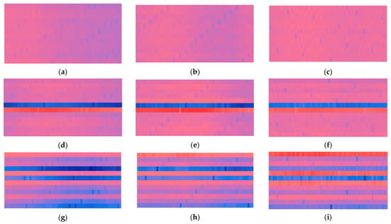
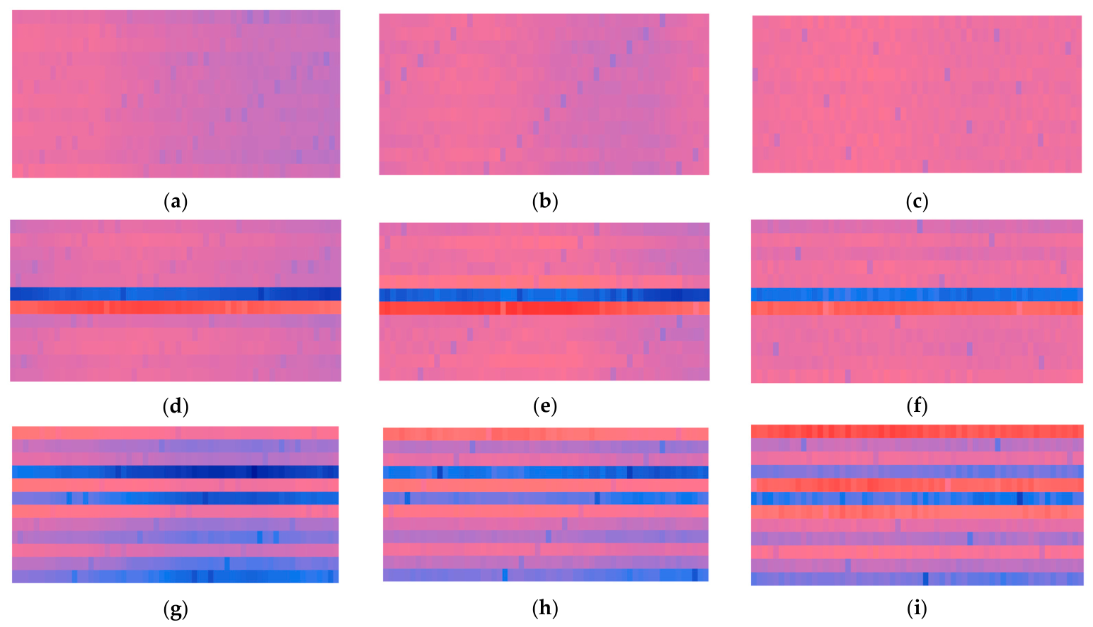
Figure 15 presents the heat maps of Channel 1 at different rotational speeds under different operating conditions. Under the healthy condition, the maps lie in the middle of the color scale and appear as a nearly uniform mid-tone, with no evident stripes or colour fluctuations: the twelve blade spacings recorded in each revolution remain stable and show no anomaly, and the features are highly consistent from one revolution to another. Under the tenon-root crack condition, clearly visible horizontal stripes emerge, including a comparatively prominent bright red band and a distinct blue band. Under the rub-impact condition, the maps exhibit multiple alternating red and blue horizontal stripes, the stripes being more numerous and the fluctuations more frequent. The fault characteristics of rub-impact are therefore more complex, and the resulting signal anomalies manifest themselves as denser and more irregular fluctuation patterns over successive revolutions.
Figure 15.
Heatmap of Channel 1 under different rotational speeds and operating conditions. (a) 500 rpm Healthy; (b) 1000 rpm Healthy; (c) 1500 rpm Healthy; (d) 500 rpm Crack; (e) 1000 rpm Crack; (f) 1500 rpm Crack; (g) 500 rpm Rub; (h) 1000 rpm Rub; (i) 1500 rpm Rub.
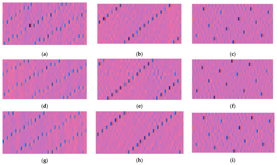
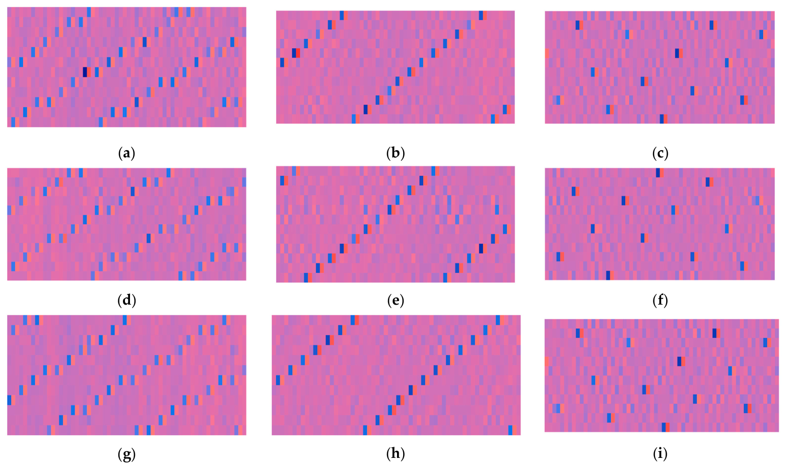
Figure 16 presents the heatmaps of Channel 2 under different operating conditions at different rotational speeds. In general, the heatmaps of the three operating conditions exhibit a high degree of similarity in terms of macroscopic structure and texture distribution, all displaying periodic oblique stripe features, making effective differentiation by human visual inspection very difficult. Nevertheless, the features of Channel 2 still contain rich high-dimensional structural information, and potential differences exist among different fault states in aspects such as feature distribution, intensity variation, and spatial correlation. Such differences are nonlinear and implicit in nature—difficult to identify through direct observation, yet capable of being captured and utilized by deep learning models. Therefore, although the differences in the Channel 2 heatmaps are not visually conspicuous, they still contain discriminative information of significant value for fault diagnosis.
Figure 16.
Heatmap of Channel 2 under different rotational speeds and operating conditions. (a) 500 rpm Healthy; (b) 1000 rpm Healthy; (c) 1500 rpm Healthy; (d) 500 rpm Crack; (e) 1000 rpm Crack; (f) 1500 rpm Crack; (g) 500 rpm Rub; (h) 1000 rpm Rub; (i) 1500 rpm Rub.
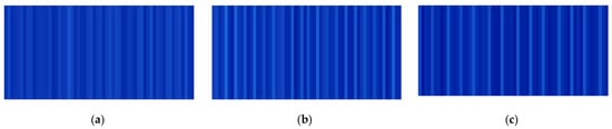
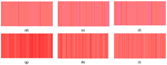
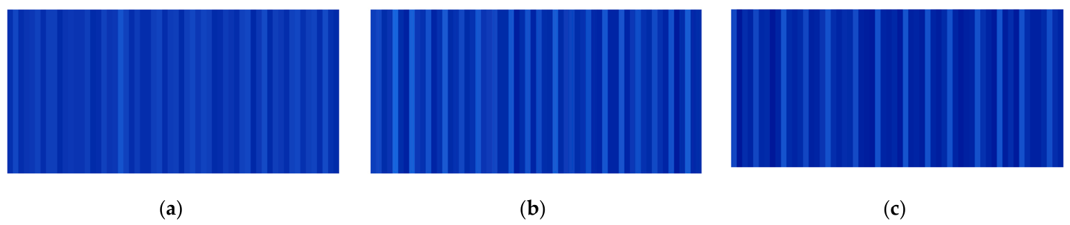
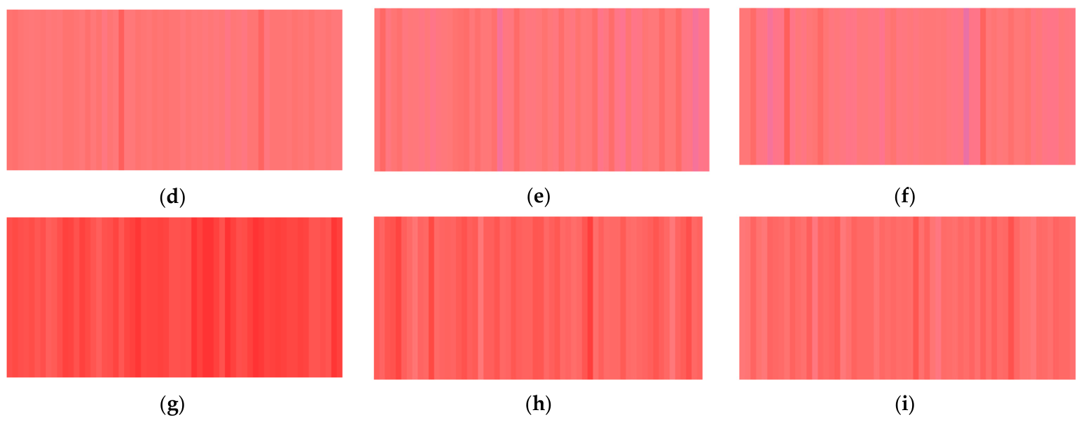
Figure 17 presents the heatmaps of Channel 3 under different operating conditions at different rotational speeds. Under the healthy condition, the heatmaps exhibit an overall uniform dark blue color, with only faint periodic textures. This indicates that the spatial coefficient of variation remains at a stable and low level, and the dispersion degree of blade spacings across revolutions maintains a high degree of consistency. Under the tenon-root crack condition, the heatmaps transition to a pink-red background with clearly visible textures. This suggests that the spatial coefficient of variation increases overall and exhibits periodic fluctuations, reflecting the influence of crack faults on the dispersion degree of blade spacings. Under the rub-impact condition, the heatmaps display a vivid red overall, with denser textures and more pronounced color fluctuations. This indicates that the spatial coefficient of variation values are relatively large and fluctuate frequently, demonstrating the strong interference of rub-impact faults on the spatial coordination of the bladed disk system.
Figure 17.
Heatmap of Channel 3 under different rotational speeds and operating conditions. (a) 500 rpm Healthy; (b) 1000 rpm Healthy; (c) 1500 rpm Healthy; (d) 500 rpm Crack; (e) 1000 rpm Crack; (f) 1500 rpm Crack; (g) 500 rpm Rub; (h) 1000 rpm Rub; (i) 1500 rpm Rub.
In summary, by transforming one-dimensional time-series signals into ECC–ΔS–SCV maps and visualizing them, this study has successfully converted abstract fault mechanisms into intuitive and identifiable spatio-temporal image patterns. This result provides compelling visual validation of the physical rationale and diagnostic potential of the multi-channel feature design. The three channels contribute in a complementary manner: Channels 1 and 3 make the fault patterns directly discernible in the maps—Channel 1 through localized horizontal stripes at the faulty blade spacing and Channel 3 through the overall level of the spatial coefficient of variation—whereas the discriminative information of Channel 2 is implicit and becomes exploitable only through deep-learning-based feature extraction. Together, they supply the subsequent deep learning model with structurally clear, information-dense, and pattern-explicit inputs, thereby establishing the data foundation for high-accuracy classification.
4.3. Analysis of CBAM-ResNet18 Diagnostic Results
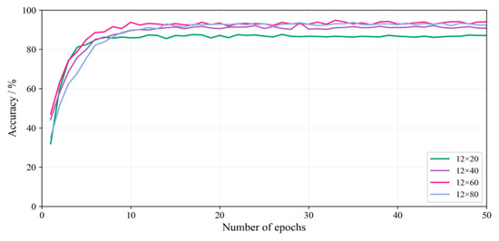
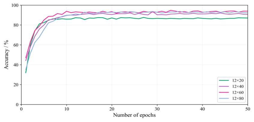
When the ECC–ΔS–SCV map is used as the model input, the input size determines how much temporal context each sample carries and therefore affects the classification accuracy. Figure 18 presents the accuracy curves with respect to the number of training epochs for different input sizes; following the conventional notation for image dimensions, the sizes are given in the columns × rows format. All curves converge within approximately 10 epochs. The final accuracy is lowest for the 12 × 20 size (86.6%), whereas the 12 × 40, 12 × 60 and 12 × 80 sizes reach 91.1%, 93.4% and 92.8%, respectively. Increasing the window from 40 to 60 revolutions brings a clear gain, whereas a further increase to 80 revolutions yields no additional benefit while raising the computational cost. The input size is therefore fixed at 12 × 60, i.e., a window of 60 consecutive revolutions. It should be emphasized that this comparison is conducted on the validation split: the input size is not chosen using the test split, which is reserved exclusively for the final evaluation.
Figure 18.
Relationship between image size and classification accuracy.
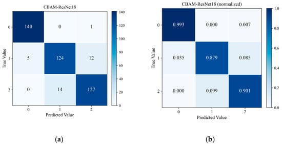
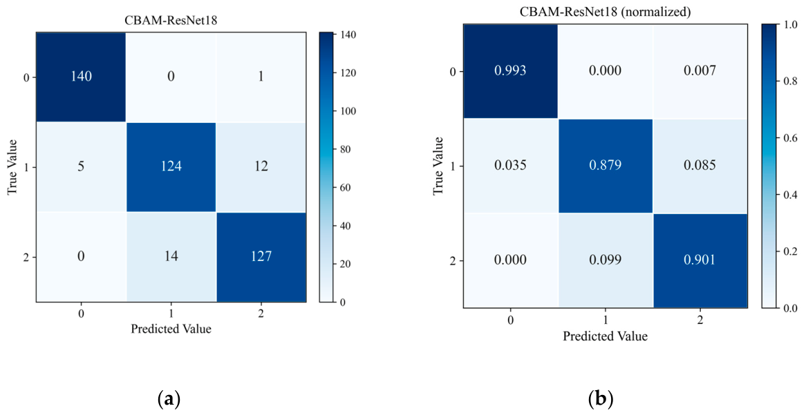
Figure 19 presents the confusion matrices of the CBAM-ResNet-18 model on the test set at 1000 rpm (a representative single run is shown; the statistics over ten runs are given in Table 3). Figure 19a shows the sample counts, and Figure 19b shows the row-normalized values. The horizontal and vertical axes represent the predicted and true labels, respectively, where 0, 1 and 2 correspond to the healthy, tenon-root crack and rub-impact conditions. As shown in Figure 19a, the test set contains 423 samples in total, with 141 samples per class. The model correctly identifies 140 healthy samples, 124 tenon-root crack samples and 127 rub-impact samples, giving an overall accuracy of 92.43%. A total of 32 misclassifications occur: one healthy sample is classified as rub-impact; among the crack samples, five are classified as healthy and twelve as rub-impact; and fourteen rub-impact samples are classified as crack. Figure 19b reports the recall of each class: 99.3% for the healthy condition, 87.9% for the tenon-root crack and 90.1% for rub-impact. The healthy condition is identified most reliably, whereas the confusion is concentrated between the crack and rub-impact conditions.
Figure 19.
Confusion matrix for the predictions of the CBAM-ResNet18 model at 1000 rpm. (a) Confusion matrix in sample counts; (b) normalized confusion matrix.
Table 3.
Statistics of the comparative experiments over ten repeated runs at 1000 rpm.
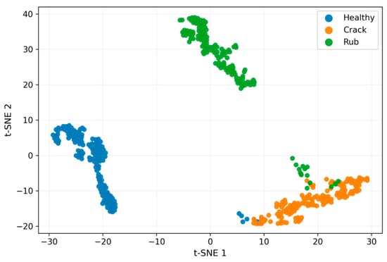
Figure 20 presents the t-SNE visualization of the features extracted from the last layer before the fully connected layer, for the 423 samples of the test set at 1000 rpm. The method projects the high-dimensional features onto a two-dimensional plane so that the distribution of the samples from different equipment states can be inspected directly. The samples of the three conditions each form a main cluster—the healthy samples on the left, the rub-impact samples in the upper region and the crack samples on the right—and the clusters are largely separated. Nevertheless, a limited number of points lie in the border regions between clusters: this occurs mainly between the crack and rub-impact clusters and, to a lesser extent, between the healthy and crack clusters. Since a two-dimensional projection inevitably discards part of the information contained in the high-dimensional features, such border points do not necessarily correspond to misclassifications.
Figure 20.
t-SNE visualization.
4.4. Analysis of Comparative Experimental Results
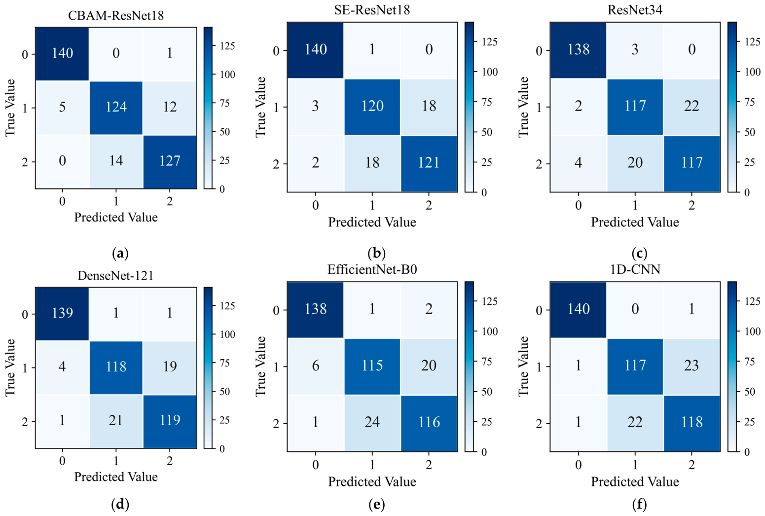
To further validate the superiority of the proposed method, comparative experiments are conducted between CBAM-ResNet-18 and five mainstream deep learning models: SE-ResNet-18, ResNet-34, DenseNet-121, EfficientNet-B0 and 1D-CNN. All compared models are evaluated under the same dataset split and the same training configuration and receive the complete ECC–ΔS–SCV map. For the 1D-CNN the map is rearranged along the revolution axis, so that the twelve blade spacings and the three channels form the 36 input channels and the 60 revolutions the sequence length (36 × 60); the network architecture is therefore the only difference between the compared models. The 1D-CNN is deliberately kept compact: three 1D convolutional blocks (kernel lengths 5, 3 and 3 with 32, 64 and 128 channels, each followed by batch normalization and max-pooling), global average pooling and a fully connected classifier.
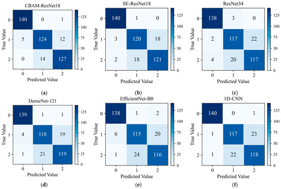
Figure 21 presents the confusion matrices of the six methods on the test split at 1000 rpm (a representative single run is shown; the statistics over the ten repeated runs are given in Table 3). The proposed CBAM-ResNet-18 achieves the highest accuracy: nearly all healthy samples are correctly identified, and the remaining errors are confined almost entirely to the crack and rub-impact classes. SE-ResNet-18 ranks second in accuracy, yet its crack–rub-impact confusion remains clearly higher than that of the proposed method; ResNet-34, DenseNet-121 and EfficientNet-B0 all yield lower accuracy than the proposed method, with ResNet-34 and EfficientNet-B0 showing the most severe crack–rub-impact confusion. The accuracy of the 1D-CNN is close to that of DenseNet-121.
Figure 21.
Confusion matrix for comparative experiments. (a) CBAM-ResNet18; (b) SE-ResNet18; (c) ResNet34; (d) DenseNet-121; (e) EfficientNet-B0; (f) 1D-CNN.
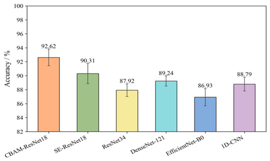
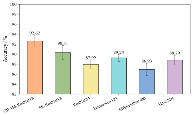
Figure 22 presents the average accuracy of each model over ten repeated runs at 1000 rpm (the partition is kept fixed and only the random seeds are varied). The proposed method attains the highest mean accuracy, 92.62 ± 1.19%, and the complete statistics are summarized in Table 3. Its advantage over every compared model is statistically significant (two-sided paired t-test over the ten runs, p < 0.001 in all cases), and the same ordering holds for the macro-averaged precision, recall and F1 score and for the per-class sensitivity of the crack and rub-impact conditions.
Figure 22.
Average accuracy in comparative experiments at 1000 rpm (mean ± standard deviation over ten repeated runs).
All models, including the 1D-CNN, use the same ECC–ΔS–SCV map; for the 1D-CNN, the map is rearranged as a 36 × 60 sequence.
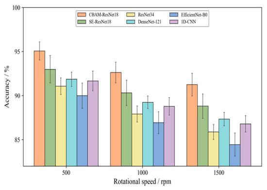
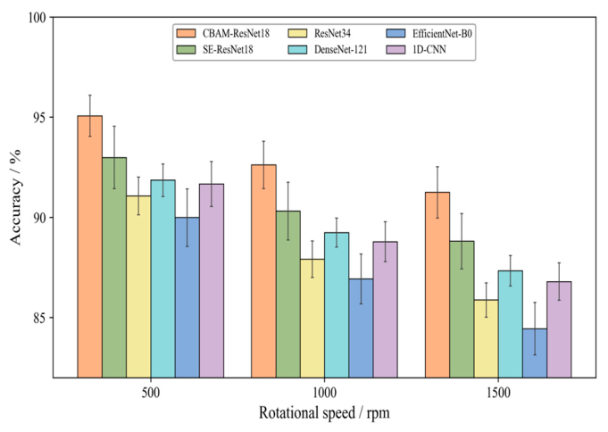
Figure 23 compares the average accuracy of each model over ten repeated runs at 500, 1000 and 1500 rpm. The proposed CBAM-ResNet-18 maintains the highest accuracy at all three speeds.
Figure 23.
Average accuracy in comparative experiments under different rotational speeds (mean ± standard deviation over ten repeated runs).
4.5. Analysis of Ablation Experiment Results
To investigate the necessity of each component in the proposed method, ablation experiments are conducted in this section. As listed in Table 4, the CBAM attention module, the SCV spatial coordination feature channel, the ΔS first-order difference feature channel and the ECC correction preprocessing are removed individually, yielding configurations E2–E5; a sixth configuration, E6, retains only the ECC channel while the attention network is kept unchanged; and two further configurations, E7 and E8, retain only the channel-attention branch and only the spatial-attention branch of CBAM, respectively, with all three feature channels kept unchanged. All eight configurations share the same dataset split and training configuration, and each is repeated ten times with the partition kept fixed and only the random seeds varied; the resulting statistics are summarized in Table 5.
Table 4.
Ablation experiment setup.
Table 5.
Statistics of the ablation experiments over ten repeated runs at 1000 rpm.
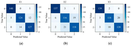
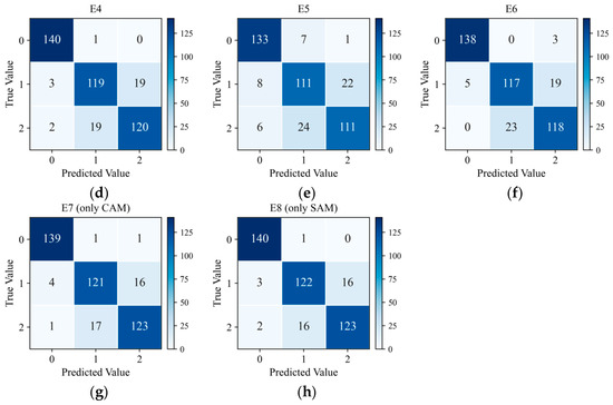
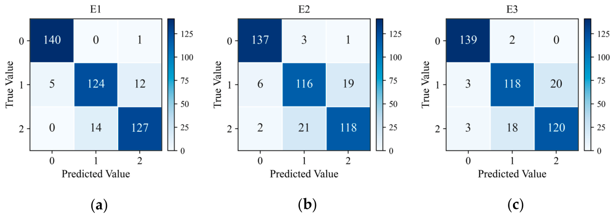
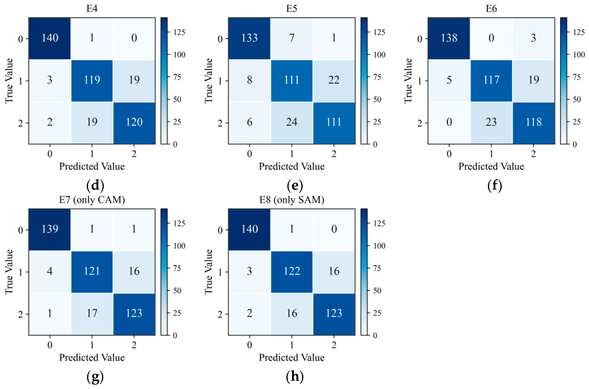
Figure 24 presents the confusion matrices of the eight configurations at 1000 rpm on the test split (a representative single run is shown; the statistics over ten runs are given in Table 5). In the complete configuration E1, the healthy condition is identified almost perfectly, and the remaining errors are confined almost entirely to the crack and rub-impact classes. Removing any component aggravates this confusion, but to different extents. Removing CBAM (E2) lowers the sensitivity of the crack and rub-impact classes by 5.6 and 6.2 percentage points (pp), respectively, and simultaneously introduces both false positives and false negatives for the healthy condition. Removing the SCV channel (E3) or the ΔS channel (E4) lowers the sensitivity of both fault classes by 4.2–5.1 pp, with a slightly stronger effect on the rub-impact class; when only the ECC channel is retained (E6), the sensitivity of the crack and rub-impact classes falls to 83.4% and 84.2%, respectively. Removing the ECC correction (E5) causes by far the most severe degradation, with the sensitivity of both fault classes falling below 80% and that of the healthy condition also dropping to 94.3%. Retaining a single attention branch degrades the performance much less than removing the module altogether: keeping only the spatial-attention branch (E8) leaves the healthy condition essentially unaffected and the two fault classes at 86.7% and 87.3%, whereas keeping only the channel-attention branch (E7) gives 98.9%, 85.8% and 86.9%, respectively.
Figure 24.
Confusion matrix for ablation experiments. (a) E1; (b) E2; (c) E3; (d) E4; (e) E5; (f) E6; (g) E7; (h) E8.
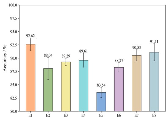
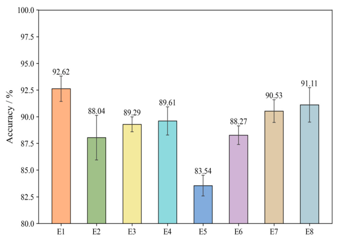
Figure 25 presents the average accuracy of the eight configurations over ten repeated runs at 1000 rpm; the corresponding mean ± standard deviation, confidence intervals and p-values are given in Table 5. The complete configuration E1 attains the highest mean accuracy, 92.62 ± 1.19%. Removing CBAM (E2) reduces it to 88.04 ± 2.09%, a decrease of 4.58 pp; removing SCV (E3) and ΔS (E4) gives 89.29 ± 0.70% and 89.61 ± 1.32%, decreases of 3.33 pp and 3.01 pp; and removing ECC (E5) gives 83.54 ± 0.97%, a decrease of 9.08 pp. Retaining only the ECC channel (E6) yields 88.27 ± 0.88%, comparable to and slightly above E2 (88.04%), indicating that the two auxiliary channels together contribute at a level comparable to that of the attention module, and that the ECC baseline alone is insufficient. The degradation caused by removing ECC is roughly twice that caused by removing the next most influential component, indicating that error compensation is the most critical step in the preprocessing pipeline. Retaining a single attention branch degrades the accuracy much less than removing the module as a whole: the spatial-attention branch alone (E8) reaches 91.11 ± 1.61% and the channel-attention branch alone (E7) 90.53 ± 1.07%. Since the gains of the two branches relative to E2, 3.07 pp and 2.49 pp, sum to more than that of the complete module, 4.58 pp, the two branches appear to carry partially overlapping information rather than contributing additively. A two-sided paired t-test over the ten runs gives p < 0.001 for every ablated configuration except E8, whose deficit of 1.51 pp is marginal at p = 0.050.
Figure 25.
Average accuracy in ablation experiments at 1000 rpm (mean ± standard deviation over ten repeated runs).
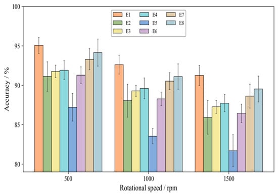
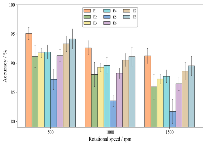
Figure 26 compares the average accuracy of the eight configurations at three rotational speeds, 500, 1000 and 1500 rpm, over ten repeated runs. For all configurations the accuracy decreases with increasing speed, and E1 remains the highest at every speed. The cross-speed drop nevertheless varies markedly with the configuration: E1 shows the smallest drop, 3.82 pp between 500 and 1500 rpm, and E5 the largest. The ordering is identical at all three speeds, from E1 down to E5, with E6 staying slightly above E2 throughout by 0.17–0.51 pp. All configurations underperform E1 at every speed, confirming the necessity of each component under multi-speed conditions.
Figure 26.
Average accuracy in ablation experiments under different rotational speeds (mean ± standard deviation over ten repeated runs).
4.6. Analysis of Cross-Speed Generalization
The experiments in Section 4.4 and Section 4.5 evaluate each model at the rotational speed at which it was trained. This setting identifies the best configuration under a matched operating condition, but it does not show whether the learned representation transfers to a speed that was never seen during training. To assess this, a leave-one-speed-out (LOSO) protocol is adopted: the proposed model is trained on the records of two rotational speeds and tested on the held-out speed, and the procedure is repeated three times so that 500, 1000 and 1500 rpm each serve once as the unseen speed. In each fold the training set contains 1746 windows drawn from the training segments of the two source speeds (291 windows per class per speed) and the test set contains the 423 windows of the held-out speed; the segment-wise partition rule of Section 4.1 is applied within each speed, and no window crosses between the splits. For each fold the ECCs of the held-out speed are derived from its healthy baseline only; this mirrors commissioning practice, in which a healthy reference is acquired at the operating speed before monitoring begins, and involves no fault-labeled data from the held-out speed.
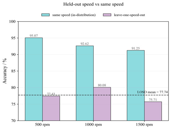
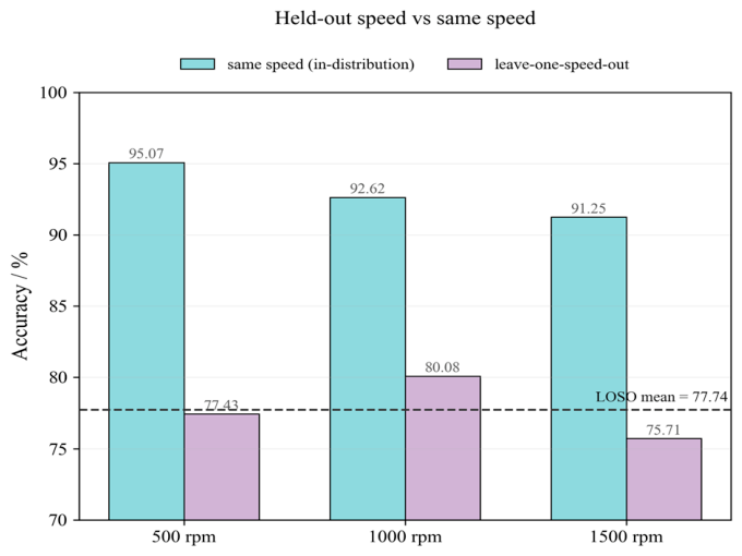
Figure 27 reports the result for the proposed CBAM-ResNet18, where the dashed line marks the mean LOSO accuracy over the three folds. The accuracy drops in all three folds, but by markedly different amounts: 17.64 pp when 500 rpm is held out, 12.54 pp when 1000 rpm is held out and 15.54 pp when 1500 rpm is held out, giving a mean drop of 15.24 pp, from 92.98% to 77.74%. The smallest drop occurs for the intermediate speed, which is bracketed by the two training speeds and therefore represents an interpolation, whereas the two extreme speeds require extrapolation and degrade more. This also explains why the fold ordering differs from that of the same-speed accuracy: 500 rpm is the easiest speed when it is included in training, but 1000 rpm is the easiest to generalize to when it is held out. The same-speed accuracy therefore reflects the intrinsic difficulty of a speed, whereas the LOSO accuracy reflects how well that speed can be predicted from the other two. The LOSO accuracy nevertheless remains between 75.71% and 80.08%, well above the 33.3% chance level, indicating that the model retains part of its discriminative ability on an unseen speed, but that this ability is far from the matched-speed performance.
Figure 27.
Leave-one-speed-out result for the proposed CBAM-ResNet18.
It should be noted that no mechanism specifically designed for cross-speed generalization—such as domain adaptation, transfer learning or speed-invariant feature learning—is incorporated in the proposed framework. The LOSO result therefore characterizes the generalization limit of the current design rather than its intended operating regime, and the conclusions of Section 4.4 and Section 4.5 should not be extrapolated to unseen rotational speeds. Improving cross-speed transferability, for example by aligning the feature distributions across speeds or by learning speed-invariant representations, is left for future work.
5. Discussion
5.1. Scope of Validity of the Reported Results
The results presented above should be read within a clearly bounded scope. All reported accuracies are obtained under matched operating conditions: the three rotational speeds are all represented in the training data, each operating condition was recorded once on a single test rig, and the reported standard deviations reflect the variation in the random seeds only. Within this scope the proposed representation and model perform well and each component contributes measurably; outside it, the conclusions cannot be transferred without further validation, as quantified below.
5.2. Limitations of the Present Study
Several limitations deserve explicit statement. First, and most importantly, the method contains no mechanism for cross-speed generalization. Under the leave-one-speed-out protocol of Section 4.6 the accuracy falls by 15.24 pp on average for the proposed model. A change in rotational speed therefore remains a genuine domain shift, and deployment at a new speed requires either retraining or fine-tuning on data from that speed. Second, the fault coverage is narrow: a single 3 mm crack on blade No. 7 and a single rub-impact condition were investigated, so the sensitivity of the method to crack length, crack location, multiple simultaneous faults and rub severity is unknown. Third, the effective sample size is smaller than the nominal one. The segment-wise split of Section 4.1 guarantees that no window crosses the training, validation or test boundary—no test window shares a single revolution with any training window—yet the 423 test windows are generated with a stride of one inside the test segment of the single recording available for each speed–condition combination, so neighboring windows remain strongly correlated, and the ten repeated runs share the same partition. Overlapping windows have been shown to yield little gain under strict, subject-independent evaluation, while they can inflate the estimated performance when they straddle a train–test boundary [27]; consistent with this, recent work on realistic evaluation of data-driven fault diagnosis recommends leakage-aware partitioning at the level of acquisition units [28]. A segment-level cross-validation would be expected to inflate the uncertainty to roughly ±2–4 pp; small differences, such as the 0.32 pp between E3 and E4 or the overlapping confidence intervals of the top-ranked comparative models, should therefore not be over-interpreted. Fourth, the ECC preprocessing is calibrated from the static deviations observed in the healthy state, so blade replacement, wear or re-assembly of the bladed disk invalidates the calibration and requires it to be repeated. Fifth, the attention mechanism is not yet interpretable in physical terms: the gains of the channel- and spatial-attention branches overlap (their sum exceeds that of the complete module), so the attention weights cannot be attributed cleanly to particular blade spacings or revolutions, and the residual confusion between the crack and rub-impact classes, whose sensitivities of 88.6% and 89.8% are well below the 99.5% of the healthy class, remains the main bottleneck.
5.3. Directions for Future Work
These limitations define the natural directions of future work. With respect to the evaluation protocol, the influence of window overlap will be quantified explicitly and non-overlapping windows adopted wherever they prove sufficient [27], and leakage-free, component-wise partitioning will be used so that windows originating from the same blade or the same recording never fall on both sides of a split, together with prevalence-independent metrics such as the macro-averaged AUROC and a multi-label formulation that admits co-occurring faults [28]. The sensitivity of the results to the provenance of the ECC baseline will also be examined, by recomputing the coefficients from the training segment alone. With respect to the method itself, transfer or domain-adaptation strategies will be investigated for unseen rotational speeds, the fault library will be extended to crack size and location as well as compound faults, the ECC baseline will be recalibrated online, and the attention weights will be analyzed so that they can be attributed to specific blade spacings and revolutions. Finally, the comparison reported in Section 4.4 evaluates alternative architectures on the same representation and therefore isolates the contribution of the network rather than that of the representation against the BTT-specific diagnostic pipelines reviewed in Section 1; a direct comparison with those methods—for example the Lomb–Scargle-based approach of Wu et al. [14] and the Bayesian hybrid strategy of Du et al. [13]—is not yet available, because they report a different diagnostic quantity (the presence and location of a crack rather than a three-class label) and were validated on different rigs and signal quantities; re-implementing them on the present dataset is an immediate next step.
6. Conclusions
The experimental results demonstrate that the proposed method achieves mean classification accuracies of 95.07%, 92.62% and 91.25% at 500, 1000 and 1500 rpm, respectively, covering the healthy, crack and rub-impact conditions, with an average of 92.98% over the three speeds. The comparative experimental results further show that CBAM-ResNet-18 outperforms the compared models—SE-ResNet-18, ResNet-34, DenseNet-121, EfficientNet-B0 and 1D-CNN—under the same data split and training configuration, validating the superiority of the proposed framework in terms of diagnostic accuracy. Ablation experiments verify the necessity of each component: removing the CBAM module, the SCV channel, the ΔS channel and the ECC preprocessing reduces the mean accuracy at 1000 rpm to 88.04%, 89.29%, 89.61% and 83.54%, respectively, and retaining only a single attention branch reduces it by a further 1.51–2.09 pp. It should be noted that all these results are obtained at the rotational speed included in training. Under the leave-one-speed-out protocol of Section 4.6, where the test speed is excluded from training, the accuracy of the proposed method still falls by 15.24 pp on average, and no mechanism for cross-speed generalization is incorporated in the present design; the conclusions above should therefore not be extrapolated to unseen rotational speeds. Further limitations are that the experiments were conducted on a single test rig with a single 3 mm crack (blade No. 7) and a single rub-impact condition. This work provides an effective new approach for bladed disk fault diagnosis in turboshaft engines under matched operating conditions.
Author Contributions
Conceptualization, S.G.; methodology, S.G., W.Y. and A.B.; investigation, Y.L. and J.C.; data curation, Y.L. and J.C.; writing—original draft preparation, Y.L. and J.C.; writing—review and editing, S.G., W.Y. and A.B.; supervision, S.G.; funding acquisition, S.G. All authors have read and agreed to the published version of the manuscript.
Funding
This work was supported by the National Natural Science Foundation of China (Grant No. 52175090), the Guangdong Basic and Applied Basic Research Foundation (Grant No. 2024A1515140143), and the Special Project in Key Fields of Guangdong Provincial Ordinary Universities (Grant No. 2022ZDZX3025).
Data Availability Statement
The data presented in this study are included in the article. The complete raw datasets generated during this research are not publicly archived because they are part of an ongoing study; further inquiries can be directed to the corresponding author.
Conflicts of Interest
The authors declare no conflicts of interest. The funding sponsors had no role in the design of the study; in the collection, analyses, or interpretation of data; in the writing of the manuscript, and in the decision to publish the results.
References
- Fathyunes, L.; Mohtadi-Bonab, M.A. A review on the corrosion and fatigue failure of gas turbines. Metals 2023, 13, 701. [Google Scholar] [CrossRef] [Scilit]
- Kim, D.; Jiang, R.; Reed, P.A.S. Microstructural and oxidation effects on fatigue crack initiation mechanisms in a turbine disc alloy. J. Mater. Sci. 2023, 58, 1869–1885. [Google Scholar] [CrossRef] [Scilit]
- Liu, H.; Sun, Y.; Wang, H.; Zhang, H. CTNet: Improving the non-stationary predictive ability of remaining useful life of aero-engine under multiple time-varying operating conditions. Measurement 2025, 243, 116345. [Google Scholar] [CrossRef] [Scilit]
- Zhu, Y.; Wang, Y.; Qiao, B.; Liu, M.; Chen, X. Blade tip timing for multi-mode identification based on the blade vibration velocity. Mech. Syst. Signal Process. 2024, 209, 111092. [Google Scholar] [CrossRef] [Scilit]
- Chen, Z.; Sheng, H.; Xia, Y.; Wang, W.; He, J. A comprehensive review on blade tip timing-based health monitoring: Status and future. Mech. Syst. Signal Process. 2021, 149, 107330. [Google Scholar] [CrossRef] [Scilit]
- Guo, X.; Liu, H.; Zhou, Z. Improving the blade tip clearance measurement method based on blade tip timing: Accounting for rotor speed variations and non-uniform blade-by-blade tip clearance. Measurement 2025, 242, 115777. [Google Scholar] [CrossRef] [Scilit]
- Fan, Z.; Li, H.; Dong, J.; Wei, D.; Cao, H.; Chen, Y. An improved mistuning identification and dynamic strain prediction method for rotating blades with application of blade tip timing technology. Mech. Syst. Signal Process. 2023, 184, 109684. [Google Scholar] [CrossRef] [Scilit]
- Witoś, M. High sensitive methods for health monitoring of compressor blades and fatigue detection. Sci. World J. 2013, 2013, 218460. [Google Scholar] [CrossRef] [Scilit] [PubMed]
- Zielinski, M.; Ziller, G. Noncontact blade vibration measurement system for aero engine application. In Proceedings of the 17th International Symposium on Airbreathing Engines, Munich, Germany, 4–9 September 2005; Volume 11, p. 244. [Google Scholar]
- Xu, J.; Qiao, B.; Liu, M.; Yang, Z.; Chen, X. Crack propagation monitoring of rotor blades using synchroextracting transform. J. Sound Vib. 2021, 509, 116253. [Google Scholar] [CrossRef] [Scilit]
- Guo, S.P.; Fan, X.M.; Wang, P.; Li, X.; Li, H. Vibration characteristics analysis of bladed disks with crack on disk outer edge. Mech. Sci. Technol. Aerosp. Eng. 2022, 41, 737–746. [Google Scholar]
- Chen, Z.; Yang, Y.; Xie, Y.; Guo, B.; Hu, Z. Non-contact crack detection of high-speed blades based on principal component analysis and Euclidian angles using optical-fiber sensors. Sens. Actuators A Phys. 2013, 201, 66–72. [Google Scholar] [CrossRef] [Scilit]
- Du Toit, R.G.; Diamond, D.H.; Heyns, P.S. A stochastic hybrid blade tip timing approach for the identification and classification of turbomachine blade damage. Mech. Syst. Signal Process. 2019, 121, 389–411. [Google Scholar] [CrossRef] [Scilit]
- Wu, S.; Wang, Z.; Li, H.; Yang, Z.; Tian, S.; Yan, R.; Wang, S.; Chen, X. Blade crack detection using blade tip timing. IEEE Trans. Instrum. Meas. 2021, 70, 6502813. [Google Scholar] [CrossRef] [Scilit]
- Guo, S.; Cao, J.; Yu, H.; Huang, X.; Li, X. Characterization and fault diagnosis of vibration characteristics of tenon disks with cracks based on blade tip timing. Meas. Sci. Technol. 2025, 36, 025010. [Google Scholar] [CrossRef] [Scilit]
- Wang, W.M.; Chen, Z.W.; Zhang, X.L.; Chen, K. Fault diagnosis method of rotor rub impact based on blade tip timing. Acta Aeronaut. Astronaut. Sin. 2022, 43, 625031. [Google Scholar]
- Wu, S.M.; Chen, X.F.; Yang, Z.B. Rotor blade rubbing fault diagnosis using blade tip timing. Aeronaut. Manuf. Technol. 2022, 65, 24–33. [Google Scholar] [CrossRef]
- Wu, S.; Tian, S.; Chen, X.; Yang, Z. Digital twin-driven blade rub-impact diagnosis using blade tip timing. Measurement 2024, 231, 114539. [Google Scholar] [CrossRef] [Scilit]
- Lin, J.; Hu, Z.; Chen, Z.S.; Yang, Y.-M.; Xu, H.-L. Sparse reconstruction of blade tip-timing signals for multi-mode blade vibration monitoring. Mech. Syst. Signal Process. 2016, 81, 250–258. [Google Scholar] [CrossRef] [Scilit]
- Huang, W.; Bian, Z.; Pan, M.; Xiao, B.; Li, A.; Hu, H.; Yang, Y.; Guan, F. A novel sparse reconstruction method for under-sampled blade tip timing signals: Integrating vibration displacement and velocity. Mech. Syst. Signal Process. 2025, 229, 112543. [Google Scholar] [CrossRef] [Scilit]
- Zhou, Y.; Liang, M.; Yue, X. Deep residual learning for acoustic emission source localization in a steel-concrete composite slab. Constr. Build. Mater. 2024, 411, 134220. [Google Scholar] [CrossRef] [Scilit]
- Zhou, Y.; Zheng, Y.; Liu, Y.; Pan, T.; Zhou, Y. A hybrid methodology for structural damage detection uniting FEM and 1D-CNNs: Demonstration on typical high-pile wharf. Mech. Syst. Signal Process. 2022, 168, 108738. [Google Scholar] [CrossRef] [Scilit]
- He, K.M.; Zhang, X.Y.; Ren, S.Q.; Sun, J. Deep residual learning for image recognition. In Proceedings of the 2016 IEEE Conference on Computer Vision and Pattern Recognition (CVPR), Las Vegas, NV, USA, 27–30 June 2016; pp. 770–778. [Google Scholar]
- Woo, S.; Park, J.; Lee, J.Y.; Kweon, I.S. CBAM: Convolutional block attention module. In Proceedings of the 15th European Conference on Computer Vision (ECCV), Munich, Germany, 8–14 September 2018; pp. 3–19. [Google Scholar]
- Kingma, D.P.; Ba, J. Adam: A method for stochastic optimization. In Proceedings of the 3rd International Conference on Learning Representations (ICLR), San Diego, CA, USA, 7–9 May 2015; pp. 1–15. [Google Scholar]
- Loshchilov, I.; Hutter, F. SGDR: Stochastic gradient descent with warm restarts. In Proceedings of the 5th International Conference on Learning Representations (ICLR), Toulon, France, 24–26 April 2017; pp. 1–16. [Google Scholar]
- Dehghani, A.; Sarbishei, O.; Glatard, T.; Shihab, E. A quantitative comparison of overlapping and non-overlapping sliding windows for human activity recognition using inertial sensors. Sensors 2019, 19, 5026. [Google Scholar] [CrossRef] [Scilit] [PubMed]
- Vieira, J.P.; Bauler, V.A.; Rosa, R.K.; Silva, D. Towards a more realistic evaluation of machine learning models for bearing fault diagnosis. Mech. Syst. Signal Process. 2026, 258, 114640. [Google Scholar] [CrossRef] [Scilit]

Disclaimer/Publisher’s Note: The statements, opinions and data contained in all publications are solely those of the individual author(s) and contributor(s) and not of MDPI and/or the editor(s). MDPI and/or the editor(s) disclaim responsibility for any injury to people or property resulting from any ideas, methods, instructions or products referred to in the content. |
© 2026 by the authors. Licensee MDPI, Basel, Switzerland. This article is an open access article distributed under the terms and conditions of the Creative Commons Attribution (CC BY) license.