Multi-Objective-Optimization-Based Optimal Sizing of Grid-Following SVG for Enhancing Transient Voltage Stability of Wind Farms Connected to Weak Grids

Abstract

When large-scale wind power bases are connected to weak grids, post-fault transient voltage recovery becomes a critical constraint on stable system operation. This paper proposes a multiobjective sizing framework for a grid-following static var generator (SVG) in which a reduced-order RK4 transient model is embedded directly in the capacity decision. The three measurement objectives are post-fault voltage recovery time, SVG investment cost, and system active-power loss, subject to minimum-voltage, recovery-time, and stability constraints. The baseline Pareto set is obtained with NSGA-II, while optimizer dependence is examined against NSGA-III and SMS-EMOA under a common evaluation budget. The grid-strength study is extended to SCR = 1.5–10.0, and the optimization scenarios retain fault-voltage levels of 0.70–0.80 p.u. A separate low-voltage-ride-through (LVRT)-aware wind-turbine model is used to evaluate active-power curtailment, reactive-current priority, and coordinated SVG-wind-turbine support. Under SCR = 2.5 and a retained fault-voltage level of 0.70 p.u., the refined capacity scan shows that enabling wind-turbine reactive support reduces the SVG capacity required to meet the same 0.019 s recovery-time target from 39 to 13 Mvar in the adopted control setting. A 10-state PMSG full-converter average-value model predicts recovery time within 1–2 ms of the reduced model for SCR = 1.5–10.0, although the reduced model overestimates post-fault voltage overshoot in very weak grids. Sequence-domain studies further quantify the additional negative-sequence, DC-link, and rotor-speed stress caused by unbalanced faults. The framework is therefore intended as a planning-stage screening tool rather than a substitute for switching-level electromagnetic-transient verification.

1. Introduction

The development of large wind and photovoltaic bases in desert, Gobi, and barren areas of China has accelerated the transition toward large-scale and centralized renewable-energy deployment. These bases are mostly located in northwestern China and transmit power over long distances to load centers [1,2]. When a wind-farm point of connection is far from strong voltage sources and the equivalent grid impedance is high, the SCR may fall below 3, or, in extreme cases, below 2, forming a weak-grid interface [3,4,5,6]. Under weak-grid conditions, voltage sensitivity, phase-locked-loop synchronization stability, and fault-ride-through capability are strongly coupled. Short-circuit faults may cause a deep PCC-voltage dip, wind-turbine protection actions, and cascading disconnection risks [7,8,9,10,11]. The transient stability and low-voltage ride-through of DFIGs and other wind-turbine technologies have been extensively studied [12,13,14,15,16]. A STATCOM/SVG can provide fast dynamic reactive-power support and is an important means of improving post-fault voltage recovery; however, its effectiveness is affected by the SCR, control bandwidth, current limitation, and interactions among multiple converters [17,18,19]. Grid codes generally require wind farms to provide fault ride-through, dynamic reactive power, and voltage regulation [20]. Therefore, capacity sizing based only on steady-state reactive-power balance cannot fully represent the post-fault dynamic security margin of a weak grid.

Existing reactive-power compensation planning commonly starts from steady-state power flow, capacity cost, or static voltage indices [21,22], whereas post-fault dynamic recovery in a weak grid is also influenced by converter control and current-limiting mechanisms [23]. To address this issue, post-fault voltage recovery time, SVG investment cost, and system active-power loss are simultaneously included as optimization objectives, while the post-fault minimum-voltage threshold, recovery-time limit, and system stability are imposed as hard constraints. The resulting multiobjective model [24] explicitly represents dynamic voltage-recovery performance in the capacity decision. Existing research on multi-objective SVG optimal configuration primarily focuses on steady-state voltage deviation, grid losses, and investment costs as optimization objectives; meanwhile, studies that incorporate post-fault voltage recovery time as an independent explicit objective function within an evolutionary optimization framework, combined with simplified transient simulation, remain relatively limited.

Incorporating transient stability into reactive-power sizing normally requires a large number of time-domain simulations. Direct use of a high-fidelity electromagnetic-transient model would substantially increase the computational burden of evolutionary optimization [25]. To balance computational efficiency and key dynamics, this study develops a simplified transient model based on the fourth-order Runge–Kutta method. Python 3.10.20. is used to represent the SVG dual-loop PI control, current limitation, and fault-voltage clamping, and the model is coupled with the pymoo platform [26], using the NSGA-II algorithm [27], enabling a single optimization run to evaluate a large number of candidate solutions.

Grid strength and fault scenarios change converter stability boundaries and admissible compensation capacity [28], so a sizing conclusion obtained under a single operating condition cannot be directly generalized. The present study therefore examines weak, medium, normal, and strong-grid references over SCR = 1.5–10.0. The optimization scenarios use retained fault-voltage levels of 0.70–0.80 p.u., while separate validation studies examine a deeper transient disturbance and balanced/unbalanced fault patterns. Multiobjective performance indicators are then used to analyze the tradeoffs among recovery time, investment cost, active-power loss, optimizer dependence, and model-form uncertainty [29,30].

In summary, the present study addresses four linked planning questions: (1) how transient-voltage recovery can be embedded directly in SVG capacity optimization; (2) how the Pareto front changes from very weak to strong-grid references and with fault severity; (3) how wind-turbine LVRT control and coordinated reactive support alter the SVG capacity requirement; and (4) how sensitive the conclusions are to optimizer choice, a higher-order PMSG average-value model, and unbalanced fault conditions. The reduced-order model remains the computational engine of the repeated optimization, whereas the higher-order models are used as targeted model-form cross-check layers outside the optimizer.

Accordingly, the contribution is not a new evolutionary algorithm but a traceable planning workflow that links transient screening, multiobjective sizing, and staged validation. Specifically, the framework (i) treats post-fault recovery time as an explicit objective together with cost and active-power loss; (ii) performs cross-scenario sizing over SCR = 1.5–10.0 and multiple retained fault-voltage levels; (iii) quantifies the influence of LVRT-aware wind-turbine reactive support and coordinated control on the required SVG rating; (iv) benchmarks NSGA-II against NSGA-III and SMS-EMOA using common HV/IGD+ definitions and the same evaluation budget; and (v) cross-checks the reduced model against a 10-state PMSG average-value model and a sequence-domain balanced/unbalanced-fault model. These layers improve the robustness and traceability of preliminary SVG sizing while preserving the distinction between planning-stage average-value models and final switching-level EMT verification.

2. Overall Solution Framework

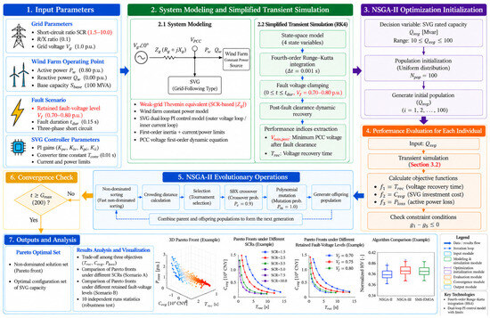
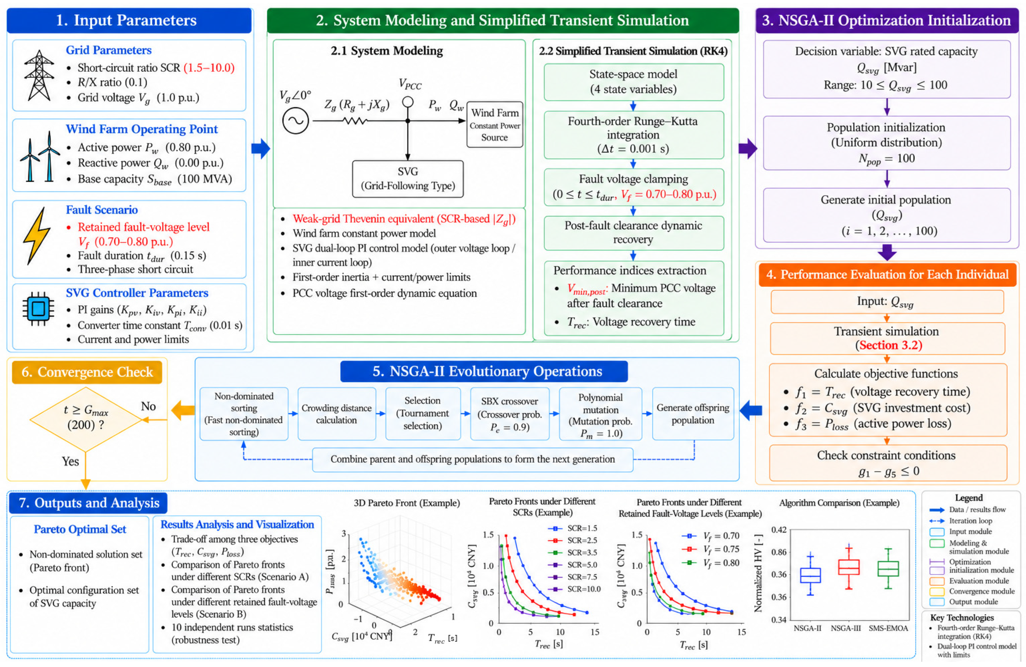
To obtain a reasonable SVG capacity for a wind farm connected to a weak grid, an integrated research framework combining transient simulation and multiobjective optimization is constructed, as shown in Figure 1.

Figure 1. Multiobjective SVG sizing framework for a weak-grid-connected wind farm with transient-voltage stability constraints.

The main procedure is as follows:

• Parameter input: Specify the grid SCR, wind-farm operating parameters, retained fault-voltage level, fault duration, and SVG control parameters.
• System modeling and simplified transient simulation: Establish the weak-grid, wind-farm, and SVG models and compute the PCC-voltage response using the fourth-order Runge–Kutta method.
• Optimization initialization: Define the SVG capacity decision variable, decision bounds, population size, and initial population.
• Individual performance evaluation: Simulate each candidate SVG capacity, calculate recovery time, investment cost, and active-power loss, and check the transient constraints.
• NSGA-II evolutionary operations: Perform nondominated sorting, crowding-distance calculation, tournament selection, crossover, mutation, and offspring generation.
• Convergence check: Continue the evolutionary loop if the maximum generation has not been reached; otherwise, terminate the optimization.
• Outputs and analysis: Obtain the Pareto-optimal set and compare sizing results under different SCRs, retained fault-voltage levels, controller assumptions, optimization algorithms, and validation models.

Figure 1 divides the sizing process into seven interconnected modules for parameter input, system modeling and simplified transient simulation, optimization initialization, individual performance evaluation, evolutionary operations, convergence checking, and outputs/analysis. Each candidate SVG’ capacity is evaluated by the RK4 transient simulation to calculate the PCC-voltage trajectory and SVG reactive-power output. The resulting recovery time, investment cost, active-power loss, and constraint values are fed back to the optimizer. The main NSGA-II sizing loop is supplemented by cross-scenario SCR/fault comparisons, optimizer benchmarking, LVRT-aware coordinated-control studies, a higher-order PMSG average-value model-form cross-check, and sequence-domain balanced/unbalanced-fault analysis.

3. Research Methodology

3.1. System Modeling

3.1.1. Wind-Farm Model

The wind farm is represented by an aggregated single-machine equivalent at the point of common coupling (PCC), while the impedance and power loss of the internal collection network are neglected. On the transient time scale considered here (seconds), the mechanical dynamics of the wind turbines are much slower than the electromagnetic-transient process. The wind farm is therefore represented as a constant-power source, and its power injection at the PCC is expressed as follows:

$$P_{wf}=P_w,Q_{wf}=Q_w$$

(1)

where $P_{wf}$ and $Q_{wf}$ denote the active and reactive powers, respectively, injected by the wind farm into the PCC in per-unit values, with the rated wind-farm capacity Sbase used as the power base.

In this study, the wind farm operates at unity power factor and does not participate in grid reactive-power regulation. Its operating point is set as follows:

$$P_w=0.80\mathrm{p}.\mathrm{u}.,Q_w=0\mathrm{p}.\mathrm{u}.$$

(2)

This setting isolates the effect of SVG capacity on transient voltage recovery. During low-voltage ride-through, actual wind turbines may use different active-power curtailment, reactive-current priority, and current-limiting strategies, depending on the turbine type, controller, and grid code. Accordingly, modeling the wind farm as a constant-power source is a computational simplification adopted for the baseline optimization rather than a universally applicable operating rule.

To isolate the effect of SVG capacity during repeated optimization, the constant-power representation is retained only inside the baseline optimization loop. It is not used as the sole validation model. In extended validation studies, an LVRT-aware converter representation enforces reactive-current priority and a total converter-current limit; active power is curtailed when the remaining d-axis current capability is insufficient. This separation preserves computational tractability for the evolutionary search while allowing the sensitivity of the sizing conclusions to wind-turbine fault controls to be quantified explicitly.

3.1.2. Weak-Grid Model

The weak grid is represented by a Thevenin-equivalent circuit, and its strength is characterized by the short-circuit ratio (SCR) at the point of connection. The SCR and its extended indices are widely used to assess grid strength and stability margins in converter-dominated systems. The SCR is defined as the ratio of the three-phase short-circuit capacity at the PCC to the rated wind-farm capacity:

$$\mathrm{SCR}={\displaystyle \frac{S_{sc}}{S_{wf}}}={\displaystyle \frac{V_n^2/\left|Z_g\right|}{P_w·S_{base}}}$$

(3)

where $V_n$ is the rated grid voltage (1.0 p.u.), $\left|Z_g\right|$ is the magnitude of the grid-equivalent impedance, $P_w$ is the wind-farm active-power output, and Sbase is the base capacity.

The magnitude of the grid equivalent impedance is obtained from (2) and (3) as follows:

$$|Z_g|={\displaystyle \frac{1}{\mathrm{SCR}\times P_w}}[\mathrm{p}.\mathrm{u}.]$$

(4)

In the adopted per-unit implementation, the dispatched wind-farm active-power level $P_w$ appears in the equivalent-impedance scaling. Therefore, the numerical SCR parameter should be interpreted as an operating-point grid-strength index within the reduced-order model, rather than as a project short-circuit metric that is completely independent of dispatch.

In this study, the grid impedance ratio is fixed at R/X = 0.1. The impedance magnitude is therefore decomposed into the resistance $R_g$ and reactance $X_g$:

$$X_g={\displaystyle \frac{\left|Z_g\right|}{\sqrt{1+{(R/X)}^2}}},R_g={\displaystyle \frac{R}{X}}·X_g$$

(5)

According to Equations (2)–(5), a lower SCR produces a larger $\left|Z_g\right|$ and therefore represents a weaker grid. The grid-voltage recovery time constant ${\tau }_{grid}$ is determined by the ratio of line inductance to resistance:

$${\tau }_{grid}={\displaystyle \frac{L_g}{R_g}}={\displaystyle \frac{1}{\omega ·(R/X)}}$$

(6)

where ω = 2πf is the system angular frequency. When R/X = 0.1 and f = 50 Hz, τ_grid ≈ 0.0318 s. This time constant determines the rate at which the PCC voltage converges to its steady-state value after fault clearance.

3.1.3. Grid-Following SVG Model

The grid-following SVG adopts a dual-loop PI structure consisting of an outer voltage loop and an inner current loop, together with a first-order inertia element and hard limits. The control objective is to regulate the PCC voltage to its reference value (1.0 p.u. in this study) by adjusting the reactive current injected by the SVG. Under weak-grid conditions, the phase-locked loop, outer-loop bandwidth, and current limitation can all affect synchronization stability and fault response. PLL dynamics are not explicitly represented as independent states in the reduced-order screening model and are therefore reserved for subsequent higher-fidelity verification.

Voltage Outer-Loop PI Controller:

The outer voltage loop takes the PCC-voltage error $V^{ref}$–$V_{pcc}$ as its input and produces the reactive-current reference $I_q^{ref}$ through PI regulation:

$$I_q^{ref}=K_p^v\left(V^{ref}-V_{pcc}\right)+K_i^v·x_i^{int}$$

(7)

where $K_p^v$ and $K_i^v$ are the proportional and integral gains of the outer voltage loop, respectively, and $x_v^{int}$ is the integrator state, the dynamic equation for which is as follows:

$${\displaystyle \frac{d{x}_v^{int}}{dt}}=V^{ref}-V_{pcc}$$

(8)

Current Inner-Loop PI Controller:

The inner current loop takes the deviation between the reactive-current reference $I_q^{ref}$ and the actual SVG output current $I_{svg}$ as its input and produces the modulation-current command $I_{cmd}$:

$$I_{cmd}=K_p^i\left(I_q^{ref}-I_{svg}\right)+K_i^i·x_i^{int}$$

(9)

where $K_p^i$ and $K_i^i$ are the proportional and integral gains of the inner current loop, respectively, and $x_i^{int}$ is the integrator state, the dynamic equation for which is as follows:

$${\displaystyle \frac{d{x}_i^{int}}{dt}}=I_q^{ref}-I_{svg}$$

(10)

First-Order Converter Inertia:

The response of the SVG converter and filter is approximated by a first-order inertia element, with the following input–output relationship:

$$T_{svg}·{\displaystyle \frac{d{I}_{svg}}{dt}}+I_{svg}=I_{cmd}$$

(11)

Hard-Limiting Stage:

Because of the SVG rated capacity and PCC-voltage limits, the output current and reactive power must satisfy the following hard constraints:

$$|I_{svg}|\le I_{limit}={\displaystyle \frac{Q_{svg}}{S_{base}·V_{pcc}}}$$

(12)

$$\left|Q_{svg}^{out}\right|\le Q_{svg}$$

(13)

where $Q_{svg}$ is the rated SVG capacity and the decision variable, $Q_{svg}^{out}$ is the actual reactive-power output of the SVG, and $I_{limit}$ is the current limit. During low-voltage conditions, the current command obtained from a constant-power conversion increases, but the actual converter output must remain protected by current limitation. Therefore, the limiting sequence and post-limiting control mode directly affect fault-period reactive-power support and synchronization stability. The model should explicitly distinguish between power limiting and current limiting, and this simplification should be verified in a subsequent high-fidelity model.

3.2. Simplified Transient Simulation

State-Space Model:

Equations (8), (10) and (11) are combined with the PCC-voltage dynamic equation to form a four-dimensional state-space model. The state vector is defined as follows:

$$x(t)={\left[\begin{array}{cccc}{V}_{pcc}& x_v^{int}& x_i^{int}& I_{svg}\end{array}\right]}^T$$

(14)

PCC-Voltage Algebraic Equation:

The PCC voltage is jointly determined by the grid-side voltage $V_g$ and the injected powers. According to the simplified power-flow equation,

$$V_{pcc}=V_g+{\displaystyle \frac{Q_{net}·X_g-P_{net}·R_g}{V_g}}$$

(15)

The net active and reactive powers injected into the PCC by the wind farm and the SVG are $P_{net}$ and $Q_{net}$, respectively:

$$P_{net}=P_w,Q_{net}=Q_w+Q_{svg}$$

(16)

PCC-Voltage Dynamic Equation:

The PCC voltage does not instantaneously reach the steady-state value given by (15). Instead, it converges to that value through a first-order inertia process, representing voltage recovery during the electromagnetic transient:

$${\tau }_{grid}·{\displaystyle \frac{d{V}_{pcc}}{dt}}+V_{pcc}=V_{pcc}^{ss}$$

(17)

where $V_{pcc}^{ss}$ is the steady-state PCC voltage calculated from Equation (15), and ${\tau }_{grid}$ is given by Equation (6).

Numerical Integration Method:

The differential-algebraic equation set is integrated in the time domain using the fourth-order Runge–Kutta method (RK4), with a fixed time step of Δt = 0.001 s and a total simulation time = 5.0 s. This reduced-order time-domain model is suitable for large-scale parameter sweeps but cannot replace an electromagnetic-transient model in fully representing control saturation, network electromagnetic dynamics, and protection logic. The RK4 one-step recursion is as follows:

$$x_{n+1}=x_n+{\displaystyle \frac{1}{6}}\left(k_1+2k_2+2k_3+k_4\right)$$

(18)

The slope vectors are calculated from the system differential equation dx/dt = f(x,t):

$$\begin{array}{cc}\hfill k_1& =\mathrm{\Delta }t·f(x_n,t_n)\hfill \\ \hfill k_2& =\mathrm{\Delta }t·f\left(x_n+{\displaystyle \frac{k_1}{2}},t_n+{\displaystyle \frac{\mathrm{\Delta }t}{2}}\right)\hfill \\ \hfill k_3& =\mathrm{\Delta }t·f\left(x_n+{\displaystyle \frac{k_2}{2}},t_n+{\displaystyle \frac{\mathrm{\Delta }t}{2}}\right)\hfill \\ \hfill k_4& =\mathrm{\Delta }t·f(x_n+k_3,t_n+\mathrm{\Delta }t)\hfill \end{array}$$

(19)

Fault Treatment:

During a three-phase short-circuit fault at the PCC, the PCC voltage is forcibly clamped to the retained fault-voltage level dFAULT:

$$V_{pcc}(t)=d_{FAULT},t\in [t_{fault},t_{fault}+t_{duration}]$$

(20)

After fault clearance, the system returns to the normal dynamics described by (17).

Transient-Stability Indices:

The following two key indices are extracted from the simulation results:

Post-fault minimum voltage V_min, post—the minimum PCC voltage after fault clearance, which is used in the optimization constraint:

$$V_{min}=\min \{V_{pcc}(t)\mid t>t_{fault}+t_{duration}\}$$

(21)

Voltage recovery time $T_{rec}$—the time required for the PCC voltage to first recover to 0.9 p.u. after fault clearance:

$$T_{rec}=\min \{\tau \ge 0\mid V_{pcc}(t_{fault}+t_{duration}+\tau )\ge 0.9\}$$

(22)

If the PCC voltage does not recover to 0.9 p.u. within the simulation horizon, T_rec = +∞, and the case is classified as unstable.

The above reduced-order time-domain model is intended as a planning-stage screening tool to narrow the range of candidate SVG capacities and reduce the number of subsequent high-fidelity EMT simulations required for final verification. It is not a substitute for full electromagnetic transient analysis using detailed converter models, protection logic, and network electromagnetic dynamics.

3.3. Formulation of the Multiobjective Optimization Problem

3.3.1. Decision Variable and Objectives

The decision variable is the rated SVG capacity:

$$x=Q_{svg}\in [10,100][\mathrm{Mvar}]$$

(23)

The following three objective functions are minimized simultaneously:

Objective 1: Transient voltage recovery time:

$$f_1(x)=T_{rec}(x)[s]$$

(24)

Objective 2: SVG investment cost:

The SVG investment cost C_svg consists of a capacity-dependent cost and a fixed installation cost:

$$f_2(x)=C_{svg}(Q_{svg})=c_{unit}·Q_{svg}+c_{fix}[\times {10}^4\mathrm{CNY}]$$

(25)

where the unit-capacity cost $c_{unit}$ = 5 × 10⁴ CNY/Mvar and the fixed installation cost $c_{fix}$ = 100 × 10⁴ CNY.

Objective 3: System active-power loss:

Under normal operating conditions, the system active-power loss is generated primarily by the SVG reactive current flowing through the grid resistance $R_g$:

$$f_3(x)=P_{loss}(Q_{svg})={\displaystyle \frac{P_w^2+{(Q_{svg}/S_{base})}^2}{V_{pcc}^2}}·R_g[\mathrm{p}.\mathrm{u}.]$$

(26)

where $V_{pcc}$ ≈ 1.0 p.u. under normal operation, and $R_g$ is determined by Equation (5).

3.3.2. Hard Constraints

All constraints are expressed in the unified form $g_i(x)$ ≤ 0:

Constraint 1: Post-fault minimum-voltage constraint:

In the case studies, the post-fault PCC minimum voltage is required to be no lower than 0.7 p.u. as an engineering constraint threshold. This value should not be described as a universal post-fault minimum-voltage requirement of GB/T 19963 [31]. Grid codes generally specify low-voltage ride-through capability through voltage-time profiles and dynamic reactive-power requirements:

$$g_1(x)=0.7-V_{min}^{post}(x)\le 0$$

(27)

Constraint 2: Recovery-time upper-limit constraint:

The voltage recovery time must not exceed 2.0 s (an engineering-practice requirement):

$$g_2(x)=T_{rec}(x)-2.0\le 0$$

(28)

Constraint 3: Capacity lower-bound constraint:

$$g_3(x)=10-Q_{svg}\le 0$$

(29)

Constraint 4: Capacity upper-bound constraint:

$$g_4(x)=Q_{svg}-100\le 0$$

(30)

Constraint 5: System-stability constraint:

The simulation result must satisfy the system-stability condition ($V_{pcc}$ converges to at least 0.95 p.u. at the end of the simulation):

$$g_5(x)=\left\{\begin{array}{cc}0,\hfill & Ifthesystemisstable\hfill \\ 1,\hfill & Ifthesystembecomesunstable\hfill \end{array}\right.$$

(31)

3.3.3. NSGA-II Configuration

The optimization problem is solved using the NSGA-II algorithm implemented on the pymoo platform. The parameter settings are listed in Table 1.

Table 1. NSGA-II parameter settings.

Parameter	Value	Symbol
Population size	100	Npop
Maximum generations	200	Gmax
Crossover operator	SBX	—
Crossover probability	0.9	pc
Distribution index	15	ηc
Mutation probability	1.0	pm
Distribution index	20	ηm

pymoo is a Python-based multiobjective optimization framework that provides object-oriented interfaces for problem definition, evolutionary algorithms, termination criteria, and performance indicators [26]. In the present implementation, the SVG sizing problem is defined by inheriting from pymoo’s Problem class with one decision variable (Q_svg), three objectives, five inequality constraints, and explicit lower and upper bounds. For each population, the _evaluate routine calls the transient-simulation module for each candidate capacity and writes the objective vector to F and the constraint values to G. NSGA-II is executed through pymoo.optimize.minimize with a population size of 100, a 200-generation termination criterion, duplicate-solution elimination, and a fixed random seed for a given run. A simulation-result cache is used to avoid repeated transient simulations of identical candidate capacities. Hypervolume (HV) and IGD+ are used for the multi-algorithm comparison reported in Section 4.6.2, using the common normalization and reference settings defined below.

A population size of 100 and a maximum of 200 generations are used, requiring approximately 20,000 candidate-solution evaluations per optimization run. Simulated binary crossover (SBX) uses a probability of 0.9 and a distribution index of 15 to generate offspring within an appropriate neighborhood of the parents. Polynomial mutation uses a probability of 1.0 and a distribution index of 20 to maintain population diversity and strengthen local search. The same algorithm parameters and stopping criterion are used for all scenarios so that the Pareto fronts obtained under different SCRs and retained fault-voltage levels remain comparable.

To assess optimizer dependence, the baseline problem is additionally solved using NSGA-III and SMS-EMOA. All three algorithms use the same population size (100), generation limit (200), decision bounds, constraints, and transient evaluator, and each algorithm is repeated ten times. For cross-algorithm comparison, the three objectives are normalized using the pooled objective ranges, the HV reference point is fixed at (1.1, 1.1, 1.1) in normalized objective space, and IGD+ is calculated against the nondominated union of all algorithms and runs. One-time CUDA kernel warm-up is excluded from the reported runtime so that the wall-clock comparison reflects the optimization itself.

3.4. Extended Validation Models

3.4.1. LVRT-Aware Wind-Turbine and Coordinated-Control Model

For the LVRT sensitivity study, the wind-turbine converter is represented by active- and reactive-current channels subject to a common current limit. Reactive-current support is prioritized during voltage depression, and the remaining current margin is assigned to active power. This model is used to compare the original constant-P/Q assumption with an LVRT-aware response and to evaluate coordinated SVG-wind-turbine reactive support without changing the baseline Pareto front used for the main sizing formulation.

3.4.2. PMSG Full-Converter Average-Value Model

A higher-order PMSG full-converter average-value model is constructed for a targeted model-form cross-check. The ten-state model contains the PCC voltage and SVG control states together with rotor speed, machine-side-converter power, DC-link voltage, a DC-link control integrator, and grid-side-converter d/q currents. It includes MPPT-like mechanical-electrical power coupling, DC-link energy balance, converter-current limitation, dynamic reactive-current support, and DC-link overvoltage protection. The same RK4 time step is retained to isolate model-form differences. This model is more detailed than the optimization model but is still an average-value/RMS-envelope model rather than a switching-level EMT model.

3.4.3. Sequence-Domain Model for Unbalanced Faults

To study unbalanced faults, the PMSG average-value model is extended to positive-, negative-, and zero-sequence PCC voltages and positive-/negative-sequence converter currents. The converter allocates current to positive-sequence voltage support, negative-sequence suppression, and active-power transfer under the same total-current limit; zero-sequence converter current is blocked by the assumed three-wire interface. Four retained phase-voltage patterns are examined: 3PH = (0.70, 0.70, 0.70), SLG = (0.20, 1.00, 1.00), LL = (1.00, 0.30, 0.30), and LLG = (1.00, 0.20, 0.20) p.u. The corresponding sequence components are calculated by symmetrical-component transformation rather than prescribed independently.

4. Case Studies

4.1. System Parameters and Baseline Validation

The simulation parameters of the SVG-connected wind-farm power system are listed in Table 2.

Table 2. System parameters.

Parameter	Value	Unit
Rated power of wind farm, Sbase	100	MVA
Active power of wind farm, Pw	0.80	p.u.
Reactive power of wind farm, Qw	0.00	p.u.
Grid voltage, Vg	1.00	p.u.
Grid R/X ratio	0.10	–
Proportional gain of SVG voltage outer loop, ${\mathrm{K}}_{\mathrm{p}}^{\mathrm{v}}$	0.50	–
Integral gain of SVG voltage outer loop, ${\mathrm{K}}_{\mathrm{i}}^{\mathrm{v}}$	10.0	–
Proportional gain of SVG current inner loop, ${\mathrm{K}}_{\mathrm{p}}^{\mathrm{i}}$	0.30	–
Integral gain of SVG current inner loop, ${\mathrm{K}}_{\mathrm{i}}^{\mathrm{i}}$	20.0	–
Inertia time constant of SVG, ${\mathrm{T}}_{\mathrm{svg}}$	0.01	s
Short-circuit ratio range, SCR	1.5–10.0	–

Table 2 defines the common simulation base: the system power base is 100 MVA; the wind farm operates at 0.80 p.u. active power and 0 p.u. reactive power; the grid voltage is 1.0 p.u.; and R/X is fixed at 0.10. The SVG uses the specified dual-loop PI parameters and a 0.01 s inertia time constant. Subsequent cases mainly vary the SCR, retained fault-voltage level, and SVG capacity, so the differences among scenarios can be attributed to grid strength, fault severity, and compensation capacity.

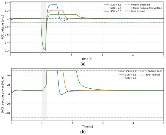
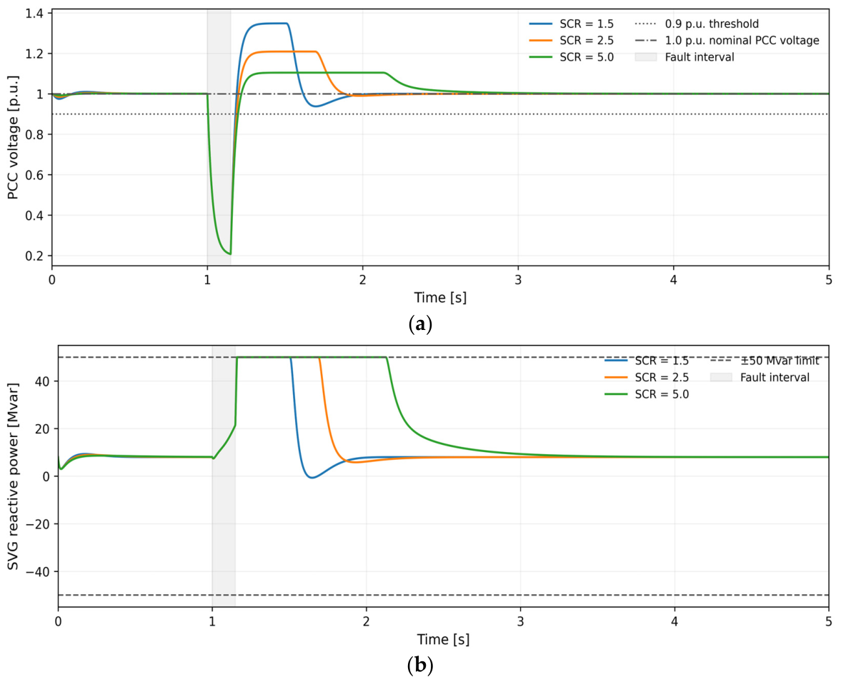
To examine the numerical behavior and physical reasonableness of the simplified transient model, three representative SCRs (1.5, 2.5, and 5.0) are first considered under a fixed SVG capacity of Q_svg = 50 Mvar, a retained fault voltage of 0.20 p.u., and a fault duration of 0.15 s. This deliberately deeper disturbance is used only for the transient-validation plot in Figure 2; the baseline Pareto optimization in Section 4.2 uses dFAULT = 0.80 p.u. Transient responses with and without the SVG are compared, and the results are summarized in Figure 2 and Table 3.

Figure 2. Deep-fault transient validation at a retained PCC fault voltage of 0.20 p.u. (a) PCC-voltage recovery under different SCRs. (b) SVG reactive-power output under different SCRs.

Table 3. Deep-fault transient-validation results.

SCR	Vmin, dist (with SVG) [p.u.]	Vmin, dist (Without SVG) [p.u.]	Trec (with SVG) [s]	Trec (Without SVG) [s]	Stable
1.5	0.2072	0.2066	0.030	0.097	Yes
2.5	0.2072	0.2068	0.038	0.080	Yes
5.0	0.2072	0.2070	0.047	0.072	Yes

For the deep-fault validation only, V_min, dist denotes the minimum PCC voltage over the complete disturbance trajectory; it is distinct from the post-fault quantity V_min, post used in the optimization constraint.

It should be noted that when SCR = 1.5, the recovery time is shorter than when SCR = 5.0; however, this does not imply that weak grids are more stable. A low SCR corresponds to a larger equivalent grid reactance X, resulting in a greater voltage rise ΔV ≈ Q_svg × X/V generated at the PCC due to the reactive current injected by the SVG; consequently, the voltage exhibits faster ‘climbing’ behavior after fault clearance. Nevertheless, as shown in Figure 2a, operating under low-SCR conditions is accompanied by more pronounced overshoot and oscillation, poorer damping characteristics, and an effectively lower system stability margin. Therefore, the ‘recovery time’ only reflects the speed of crossing the 0.9 p.u. threshold and does not equate to comprehensive transient stability.

As shown in Figure 2a, the minimum PCC voltage during the fault is approximately 0.207 p.u. in all three SCR cases, indicating essentially identical fault-voltage clamping conditions. After fault clearance, the SVG rapidly provides dynamic reactive-power support, and the PCC voltage crosses the 0.9 p.u. threshold and eventually returns to approximately 1.0 p.u. The main differences among the waveforms are the recovery rate and overshoot. For SCR = 1.5, the voltage rises most rapidly but exhibits the most pronounced overshoot and rebound; for SCR = 5.0, the waveform is smoother but takes longer to reach 0.9 p.u. Figure 2b shows that the SVG reactive-power output rapidly reaches the 50 Mvar capacity limit after fault clearance and then gradually decreases as the voltage error diminishes. The low-SCR case leaves saturation earlier but is accompanied by a brief reverse adjustment, reflecting stronger reactive-power-voltage coupling and a more sensitive control response in a weak grid.

Table 3 provides the corresponding quantitative results. Without the SVG, the recovery times for SCR = 1.5, 2.5, and 5.0 are 0.097, 0.080, and 0.072 s, respectively. With a 50 Mvar SVG, they decrease to 0.030, 0.038, and 0.047 s, corresponding to reductions of approximately 69.1%, 52.5%, and 34.7%. Thus, in the simplified model used here, a unit of SVG capacity produces a larger recovery-time improvement at lower SCR. Conversely, the difference in V_min, dist with and without the SVG is only 0.0002–0.0006 p.u., indicating that the trajectory minimum is mainly determined by the imposed fault-voltage clamp and that the SVG primarily affects the post-clearance recovery stage. All three cases ultimately converge stably.

4.2. Pareto-Front Analysis

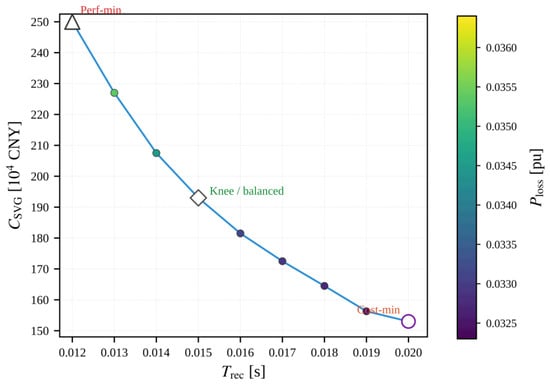
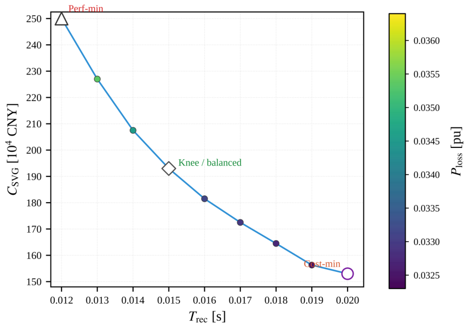
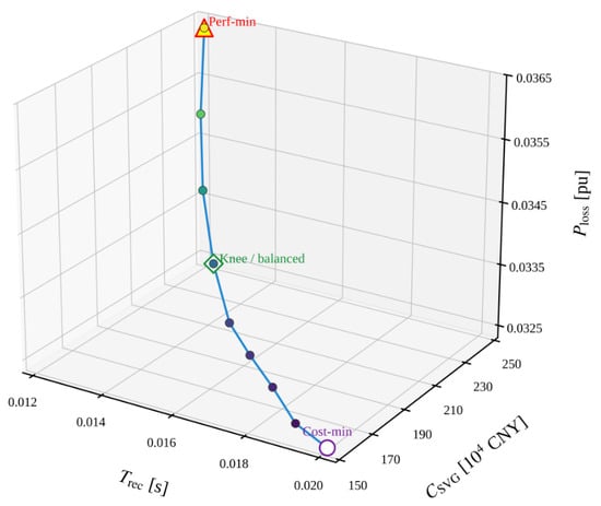
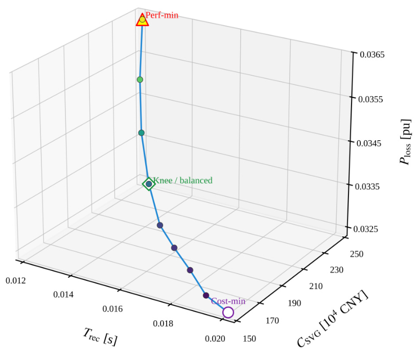
Using the simplified model described above, the NSGA-II optimization is performed for the baseline case (SCR = 2.5, dFAULT = 0.80 p.u., and tdur = 0.15 s), producing a Pareto-optimal solution set. Figure 3 and Figure 4 show the two-dimensional projection of the same nine nondominated solutions in the recovery-time-investment-cost plane and their three-dimensional representation in the objective space, respectively. Table 4 summarizes the statistical characteristics of this front.

Figure 3. Two-dimensional projection of the Pareto-optimal front for the baseline case.

Figure 4. Three-dimensional view of the Pareto-optimal front for the baseline case. Point colors encode the active-power-loss level, while the outlined markers identify the minimum-cost, knee/balanced, and best-performance solutions.

Table 4. Characteristics of the baseline Pareto front.

Metric	Value
Pareto points	9
Qsvg range	10.0–30.3 Mvar
Trec range	0.012–0.020 s
Csvg range	150.0–251.6 (×104 CNY)

The nine points in Figure 3 and Figure 4 correspond one-to-one, and each point represents the same complete nondominated three-objective solution. In the two-dimensional plot, post-fault voltage recovery time T_rec is the horizontal axis, the SVG investment cost C_svg is the vertical axis, and the color indicates the system active-power loss Ploss. In the three-dimensional plot, Ploss is displayed directly as the third coordinate. Figure 3 can therefore be regarded as the projection of Figure 4 onto the T_rec-C_svg plane. The two figures are consistent in the number of points, coordinates, and physical meaning of the solutions.

As the SVG capacity increases from 10.0 to 30.3 Mvar, the investment cost increases from 150.0 to 251.6 × 10⁴ CNY, the active-power loss increases from approximately 0.0323 to 0.0364 p.u., and the recovery time decreases from 0.020 to 0.012 s. The nine nondominated solutions are distributed in the direction of shorter recovery time, higher investment cost, and greater active-power loss. Thus, improving transient recovery performance requires both higher capital expenditure and higher operating loss, and no single solution is optimal for all three objectives.

A distinct knee point appears near T_rec = 0.015 s and C_svg = 192.5 × 10⁴ CNY in the middle of the front. Moving from the minimum-cost endpoint toward this point, additional capacity effectively shortens the recovery time. Beyond the knee and toward the best-performance endpoint, the increments in investment and loss become relatively larger while the additional improvement in recovery time gradually decreases, demonstrating diminishing marginal returns from SVG expansion. The knee point can therefore be considered a balanced candidate that accounts for transient performance, investment cost, and operating loss.

Table 4 shows that nine nondominated solutions are obtained in the baseline case. The Pareto solutions cover an SVG capacity range of 10.0–30.3 Mvar, a recovery-time range of 0.012–0.020 s, and an investment-cost range of 150.0–251.6 × 10⁴ CNY. The minimum capacity equals the lower bound of the decision variable, indicating that the 10 Mvar solution remains feasible under the current constraints. The maximum capacity corresponds to the shortest recovery time, but its increase in investment is clearly greater than the resulting incremental improvement in recovery time. Normalized HV and IGD+ are reported only in the common multi-algorithm comparison of Section 4.6.2, where the normalization range and reference point are fixed consistently.

Taken together, Figure 3 and Figure 4 and Table 4 fully demonstrate the three-objective relationship in which increasing capacity and cost shortens recovery time but increases active-power loss. If economic performance is prioritized, the minimum-cost endpoint can be selected. If rapid recovery is prioritized, higher investment and loss must be accepted. For a general engineering application, the knee-point solution in the middle of the front should be examined first.

4.3. Scenario A: Migration of the Pareto Front Under Different SCRs

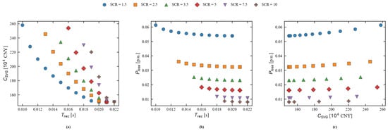
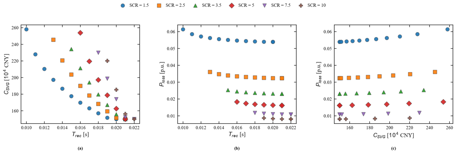
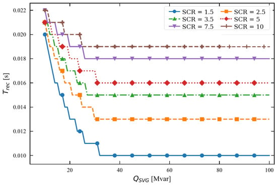
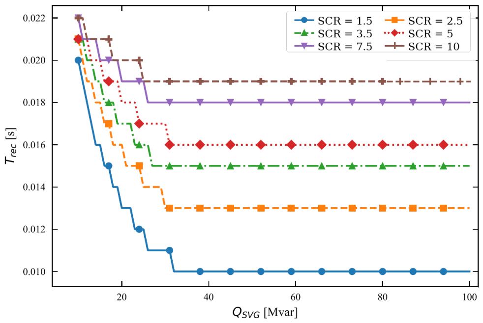
To reveal the effect of grid strength beyond the original weak-grid range, six cases with SCR = 1.5, 2.5, 3.5, 5.0, 7.5, and 10.0 are examined while dFAULT is fixed at 0.80 p.u. The first four cases retain the original weak-to-medium-grid comparison, whereas SCR = 7.5 and 10.0 provide normal/strong-grid reference cases. Figure 5 extends the Pareto comparison to all six SCR values, Figure 6 shows the corresponding Q_svg-T_rec curves, and Table 5 retains the detailed numerical ranges for the original SCR = 1.5–5.0 sizing subset.

Figure 5. Comparison of Pareto fronts over SCR = 1.5–10.0. (a) T_rec-C_svg tradeoff. (b) T_rec-Ploss tradeoff. (c) C_svg-Ploss tradeoff.

Figure 6. Relationship between SVG capacity and recovery time over SCR = 1.5–10.0, including normal- and strong-grid reference cases.

Table 5. Pareto-front characteristics for the original SCR = 1.5-5.0 sizing subset.

SCR	Pareto Points	Qsvg Range [Mvar]	Trec Range [s]	Csvg Range [×104 CNY]
1.5	10	10.0–26.4	0.010–0.019	150.0–231.8
2.5	9	10.0–30.3	0.012–0.020	150.0–251.6
3.5	7	10.0–27.8	0.014–0.020	150.0–239.2
5.0	7	10.0–33.0	0.015–0.021	150.0–264.8

Figure 5 shows that the recovery-time/cost tradeoff and the loss level remain strongly dependent on grid strength when the comparison is extended to SCR = 7.5 and 10.0. The strong-grid reference fronts exhibit lower active-power loss for comparable capacities, while the recovery-time benefit of additional SVG capacity still shows clear diminishing returns. The extension also confirms that a weak-grid sizing rule should not be extrapolated directly to normal or strong grids because the voltage sensitivity to reactive injection and the loss penalty change substantially with SCR.

Figure 6 presents the complete Q_svg-T_rec response for all six SCR values. Each curve decreases with increasing capacity and then approaches a plateau, indicating a capacity region beyond which additional SVG rating produces little recovery-time improvement. The added SCR = 7.5 and 10.0 cases provide a broader normal/strong-grid comparison and confirm that diminishing marginal benefit remains relevant outside the weak-grid range. Consequently, the onset of the plateau is a more defensible planning indicator than applying a fixed capacity multiplier across all grid strengths.

Table 5 reports the original quantitative ranges for SCR = 1.5–5.0 because these cases define the weak-to-medium-grid sizing subset used in the baseline engineering discussion. The SCR = 7.5 and 10.0 results are added as strong-grid reference cases in Figure 5 and Figure 6 to test the generality of the observed trends. Their inclusion is intended to broaden the comparison rather than to imply that the same weak-grid capacity recommendation should be used in strong grids.

4.4. Scenario B: System Robustness Under Different Retained Fault-Voltage Levels

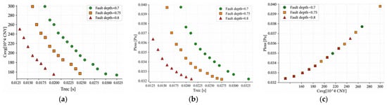
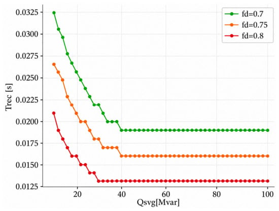
With SCR fixed at 2.5, the effect of fault severity (dFAULT = 0.70, 0.75, and 0.80 p.u.) on optimal sizing is examined. The results are shown in Figure 7 and Figure 8 and Table 6.

Figure 7. Comparison of Pareto fronts under different retained fault-voltage levels: (a) T_rec-C_svg tradeoff; (b) T_rec-Ploss tradeoff; (c) C_svg-Ploss tradeoff.

Figure 8. Relationship between SVG capacity and recovery time under different retained fault-voltage levels.

Table 6. Pareto-front characteristics under different retained fault-voltage levels.

Retained Fault-Voltage Level [p.u.]	Pareto Points	Trec Range [s]	Qsvg Range [Mvar]
0.70	15	0.018–0.032	10.0–39.8
0.75	12	0.016–0.027	10.0–31.7
0.80	9	0.012–0.020	10.0–30.3

Figure 7a shows that when dFAULT decreases from 0.80 to 0.70 p.u., the fault becomes more severe and the recovery-time-cost front shifts to the right and extends toward higher capacities. At the same investment cost, a more severe fault produces a longer T_rec. Figure 7b shows that the Pareto solutions extend into a higher Ploss region as the fault becomes more severe. This does not occur because the fault voltage directly changes the normal-operation loss formula, but because more severe faults cause higher-capacity solutions to enter the nondominated set. In Figure 7c, the cost-loss points for the three fault levels lie approximately on the same increasing curve, because both C_svg and Ploss are primarily determined by Q_svg, whereas fault severity mainly affects whether a solution becomes Pareto optimal by changing T_rec.

Figure 8 shows that all three Q_svg-T_rec curves decrease with increasing capacity and that the curve is higher for a more severe fault. At Q_svg ≈ 25 Mvar, the recovery times for dFAULT = 0.70, 0.75, and 0.80 p.u. are approximately 0.022, 0.019, and 0.014 s, respectively. The curves approach plateaus after approximately 35–40 Mvar, with plateau values of about 0.019, 0.016, and 0.013 s. Thus, a more severe fault not only lengthens the recovery time but also delays the saturation point of capacity benefit. Beyond the beginning of the plateau, further capacity expansion provides little transient-performance benefit.

Table 6 quantifies the effect of fault severity. When dFAULT decreases from 0.80 to 0.70 p.u., the number of Pareto points increases from 9 to 15, an increase of approximately 66.7%; the upper recovery-time limit increases from 0.020 to 0.032 s, an increase of 60%; and the maximum SVG capacity increases from 30.3 to 39.8 Mvar, an increase of approximately 31.4%. The minimum capacity remains 10.0 Mvar in all three cases. The present result therefore indicates that a severe fault extends the front toward longer recovery times and higher capacities rather than completely eliminating the low-capacity endpoint.

4.5. Engineering Interpretation and Traceable Capacity Selection

Based on the same nine baseline nondominated solutions shown in Figure 3 and Figure 4, Table 7 selects three representative designs—the minimum-cost solution, the best-performance solution, and the knee-point balanced solution—to illustrate design selection under different engineering preferences.

Table 7. Three representative engineering solutions.

Solution	Qsvg [Mvar]	Trec [s]	Csvg [×104 CNY]	Ploss [p.u.]	Stable
Minimum-cost solution	10.0	0.020	150.0	0.0323	Yes
Best-performance solution	30.3	0.012	251.6	0.0364	Yes
Balanced solution	18.5	0.015	192.5	0.0335	Yes

The minimum-cost solution in Table 7 lies at the low-investment, low-loss end of the Pareto front and is suitable for applications with tight budget constraints and tolerance for a longer recovery time. The best-performance solution lies at the shortest-recovery-time end and is suitable for applications requiring rapid transient voltage recovery. The balanced solution is the knee point among the nine nondominated solutions and provides a comparatively even compromise among recovery performance, equipment investment, and operating loss. All three solutions satisfy the stability constraints specified in this study.

The minimum-cost solution is Q_svg = 10.0 Mvar, T_rec = 0.020 s, C_svg = 150.0 × 10⁴ CNY, and Ploss = 0.0323 p.u. The best-performance solution is Q_svg = 30.3 Mvar, T_rec = 0.012 s, C_svg = 251.6 × 10⁴ CNY, and Ploss = 0.0364 p.u. The knee-point balanced solution is Q_svg = 18.5 Mvar, T_rec = 0.015 s, C_svg = 192.5 × 10⁴ CNY, and Ploss = 0.0335 p.u. Relative to the minimum-cost solution, the balanced solution increases investment by approximately 28.3%, shortens recovery time by 25%, and increases active-power loss by only about 3.7%. Increasing the capacity further to the best-performance solution produces larger increases in investment and loss while the marginal improvement in recovery time decreases. Therefore, when no single objective has explicit priority, the knee-point solution is a more suitable initial candidate for subsequent engineering verification.

To avoid unsupported universal safety factors, the Pareto results are not converted into broad SVG rating bands by applying an assumed engineering multiplier. Table 8 instead reports only directly traceable sizing evidence from the optimization, severe-fault study, coordinated-control scan, and strong-grid extension. A project-specific security margin should be determined only after plant-base conversion, credible-fault selection, redundancy requirements, and higher-fidelity validation are defined.

Table 8. Traceable capacity-planning evidence and its engineering interpretation.

Evidence	Studied Condition	Direct Result	Planning Interpretation
Baseline knee point	SCR = 2.5, dFAULT = 0.80	Qsvg = 18.5 Mvar; Trec = 0.015 s	Balanced initial candidate before project-specific margin
Severe-fault Pareto extent	SCR = 2.5, dFAULT = 0.70	Nondominated range extends to 39.8 Mvar	Severe faults can move the useful capacity range upward
Coordinated support	SCR = 2.5, dFAULT = 0.70, Trec* = 0.019 s	39 Mvar (SVG only) → 13 Mvar (SVG + WTG)	Dynamic turbine reactive support can reduce the required SVG rating under the adopted control
Strong-grid extension	SCR = 7.5 and 10.0	Diminishing Qsvg-Trec benefit remains visible	Do not extrapolate weak-grid rating rules to strong grids
Final project rating	Site-specific	No universal multiplier claimed	Derive margin from plant base, N→1/redundancy, credible faults, grid code, and EMT/RTDS/field validation

Note: All values in Table 8 are direct outputs or directly derived comparisons from the studied 100 MVA-base cases. No universal 1.5–2.0 security multiplier is applied in this study.

Table 8 deliberately separates optimization outputs from engineering design margins. The baseline knee point and severe-fault Pareto extent provide traceable screening values, while the coordinated-control result demonstrates that the required SVG rating is controller-dependent. The refined scan at SCR = 2.5 and dFAULT = 0.70 p.u. reduces the capacity required to meet T_rec ≤ 0.019 s from 39 Mvar for SVG-only support to 13 Mvar when wind-turbine reactive support is enabled, corresponding to a 26 Mvar (66.7%) reduction under the adopted model and controller. This percentage is scenario-specific and should not be generalized as a universal derating factor.

For a specific project, the screening result should therefore be converted into the actual plant base and then checked against the most severe credible balanced and unbalanced faults, converter-current limits, compensation redundancy, N-1 requirements, and site-specific grid-code criteria. The final equipment rating should be determined from this project-specific verification rather than from a fixed multiplier applied to the Pareto capacity.

4.6. Extended Validation and Robustness Studies

4.6.1. LVRT-Aware Wind-Turbine Response and Coordinated Support

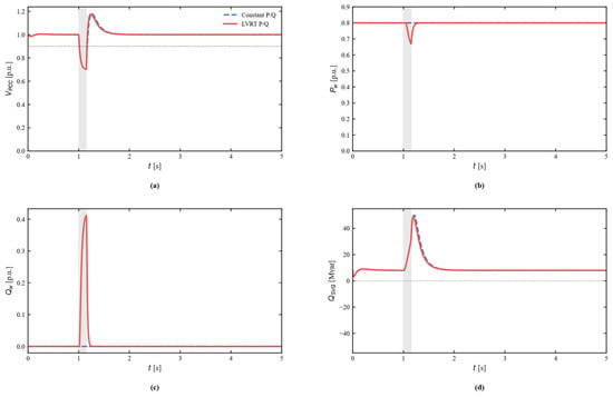
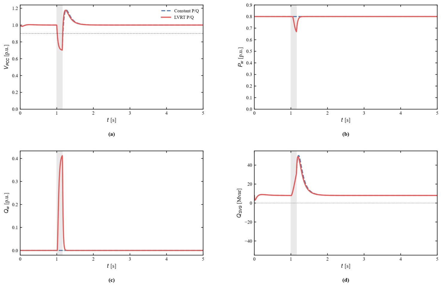
Figure 9 compares the original constant-P/Q wind-farm representation with the LVRT-aware model at SCR = 2.5, Q_svg = 50 Mvar, and dFAULT = 0.70 p.u. Dynamic turbine reactive support shortens T_rec from 0.019 to 0.014 s, while Q_w reaches approximately 0.273 p.u. The active-power reduction is small in this particular 0.70 p.u. case because the current limit is not fully occupied; deeper-fault sensitivity tests show that active-power curtailment becomes significant when reactive-current priority consumes more of the converter-current margin. Thus, the constant-power model is useful for isolating SVG sizing but does not reproduce all LVRT interactions.

Figure 9. LVRT-aware wind-turbine response at SCR = 2.5, Q_svg = 50 Mvar, and dFAULT = 0.70 p.u. (a) PCC voltage. (b) Wind-turbine active power. (c) Wind-turbine reactive power. (d) SVG reactive-power output.Grey shading denotes the fault interval; dotted reference lines indicate the 0.9 p.u. recovery threshold or the zero reference, as applicable.

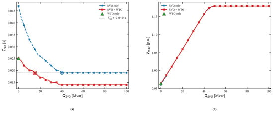
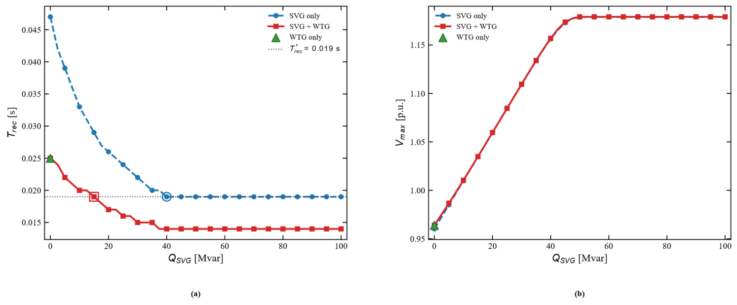
Figure 10 evaluates coordinated SVG-wind-turbine support over Q_svg = 0–100 Mvar. Using the SVG-only response at Q_svg = 50 Mvar as the common target (T_rec* = 0.019 s), the subsequent 0.5 Mvar refined scan gives a minimum SVG capacity of 39 Mvar for SVG-only support and 13 Mvar for coordinated support. The resulting 66.7% capacity reduction demonstrates the potential value of coordinated reactive-power control, but it is tied to the adopted LVRT parameters, current limits, operating point, and fault condition.

Figure 10. Coordinated SVG-wind-turbine support. (a) Recovery time versus SVG capacity, including the SVG-only, WTG-only, and coordinated cases. (b) Post-fault maximum PCC voltage versus SVG capacity.

Table 9 quantifies the trends shown in Figure 9 and Figure 10. At Q_svg = 50 Mvar and a retained fault-voltage level of 0.70 p.u., introducing LVRT-aware wind-turbine reactive support reduces T_rec from 0.019 s to 0.014 s, corresponding to a 26.3% reduction, while the peak wind-turbine reactive-power output increases from 0 to 0.273 p.u. More importantly, for the common target T_rec* = 0.019 s, the refined capacity scan reduces the required SVG rating from 39 Mvar in the SVG-only case to 13 Mvar under coordinated SVG-WTG support, i.e., a reduction of 26 Mvar or 66.7%. These values demonstrate that the required SVG capacity is strongly dependent on the wind-turbine fault-control strategy and available dynamic reactive-current support.

Table 9. Quantitative LVRT and coordinated-control results.

Metric	Reference Case	Enhanced Case	Change
Trec at Qsvg = 50 Mvar, fd = 0.70	0.019 s	0.014 s	−26.3%
Qw,max at Qsvg = 50 Mvar	0 p.u.	0.273 p.u.	Dynamic reactive support enabled
Required Qsvg for Trec* = 0.019 s	39 Mvar	13 Mvar	−26 Mvar (−66.7%)

4.6.2. Multiobjective Optimizer Comparison

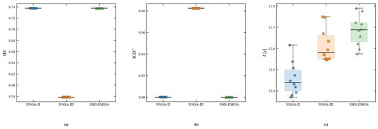
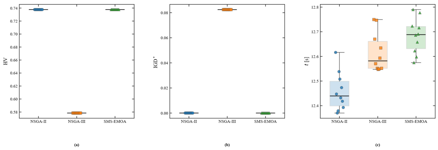
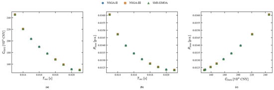
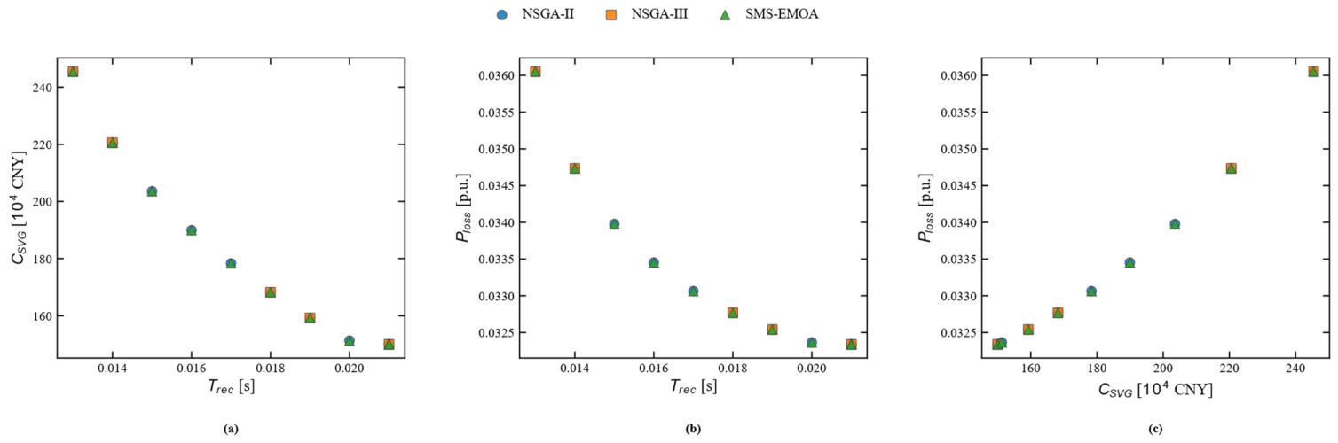
The baseline optimization is repeated ten times with NSGA-II, NSGA-III, and SMS-EMOA under the same 20,000-evaluation budget. Figure 11 compares normalized HV, IGD+, and runtime; Figure 12 overlays representative Pareto fronts. NSGA-II and SMS-EMOA produce nearly identical fronts and very similar convergence indicators, whereas NSGA-III returns a sparser nondominated set for this one-decision-variable, three-objective problem. The result supports the robustness of the reported Pareto relationship to optimizer choice; it should not be interpreted as a universal ranking of the algorithms.

Figure 11. Algorithm-comparison statistics over ten independent runs. (a) Normalized HV. (b) IGD+. (c) Runtime.

Figure 12. Representative Pareto fronts obtained by NSGA-II, NSGA-III, and SMS-EMOA under the same evaluation budget. (a) T_rec-C_svg. (b) T_rec-Ploss. (c) C_svg-Ploss.

Figure 11a shows that NSGA-II and SMS-EMOA have nearly identical normalized HV distributions, whereas NSGA-III yields a distinctly lower HV. Figure 11b shows the same pattern for IGD+: NSGA-II and SMS-EMOA remain close to zero, while NSGA-III exhibits a much larger distance from the common reference front. Figure 11c shows that the three algorithms have similar runtimes, so the difference in solution-set quality is not explained by a substantially different computational budget.

Figure 12 confirms the statistical results visually. The representative NSGA-II and SMS-EMOA solutions almost overlap in the T_rec-C_svg, T_rec-Ploss, and C_svg-Ploss planes, indicating that both algorithms recover essentially the same tradeoff surface under the common evaluation budget. The NSGA-III result is sparser, but its solutions still follow the same overall monotonic tradeoff trend, which supports the conclusion that the principal sizing relationship is not specific to NSGA-II.

Table 10 provides the quantitative basis for Figure 11 and Figure 12. NSGA-II obtains a mean normalized HV of 0.737653 and a mean IGD+ of 0.000025 with an average of 11 Pareto points, while SMS-EMOA gives an almost identical HV of 0.737660 and a slightly smaller IGD+ of 0.000018 with the same average Pareto-set size. NSGA-III yields a lower HV of 0.578421, a larger IGD+ of 0.082453, and an average of five Pareto points. The mean runtimes are close—12.46 s, 12.62 s, and 12.68 s for NSGA-II, NSGA-III, and SMS-EMOA, respectively—indicating that the observed differences mainly reflect optimizer behavior rather than unequal computational effort. Accordingly, NSGA-II and SMS-EMOA provide consistent fronts for this problem, whereas NSGA-III returns a sparser approximation under the same evaluation budget.

Table 10. Multiobjective algorithm comparison (10 independent runs).

Algorithm	HV Mean	IGD+ Mean	Pareto Points	Runtime [s]
NSGA-II	0.737653	0.000025	11.0	12.46
NSGA-III	0.578421	0.082453	5.0	12.62
SMS-EMOA	0.737660	0.000018	11.0	12.68

4.6.3. Model-Form Cross-Check with a Higher-Order PMSG Average-Value Model

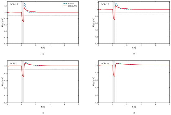
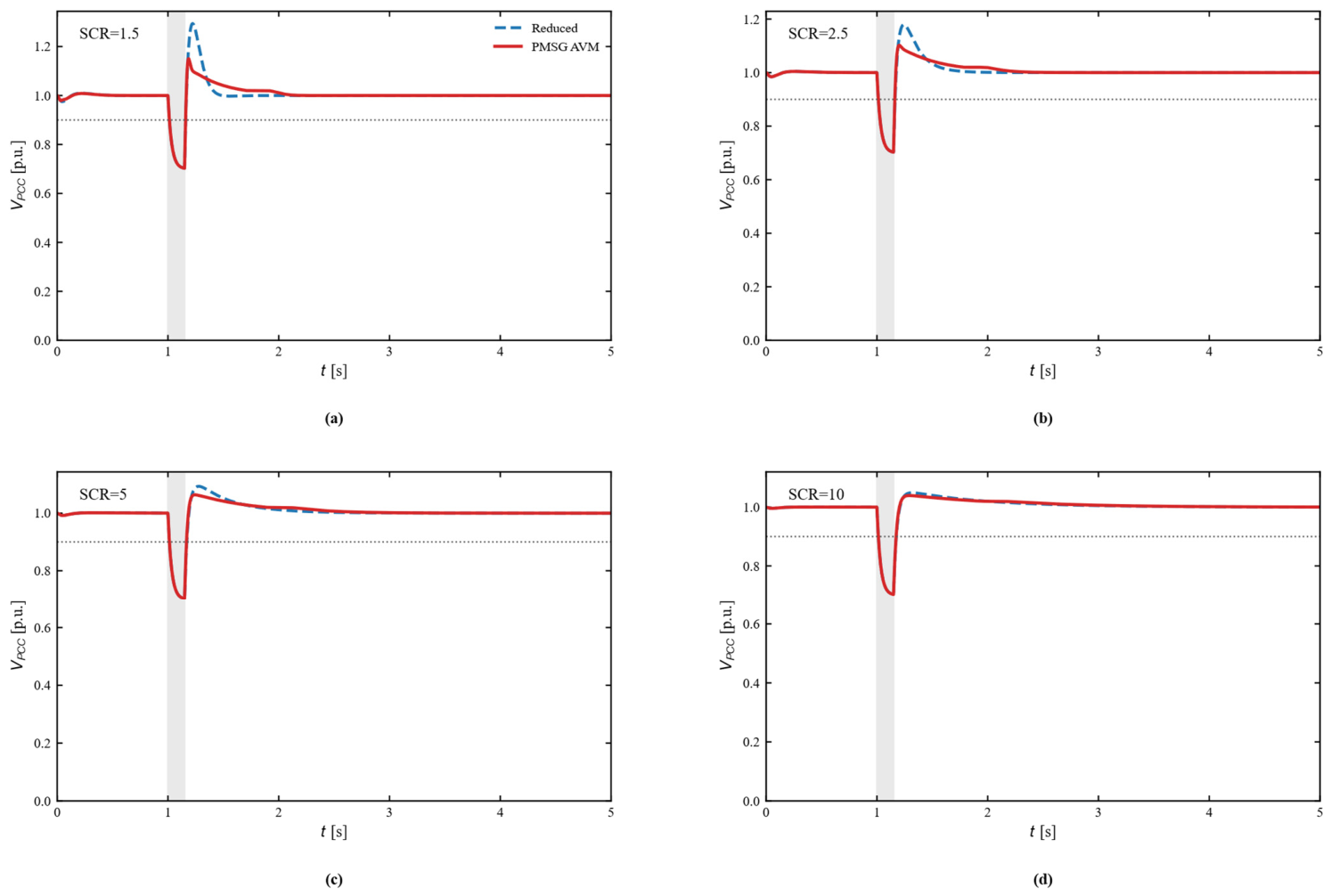
A ten-state PMSG full-converter average-value model is used to quantify model-form error at SCR = 1.5, 2.5, 5.0, and 10.0 with Q_svg = 50 Mvar and dFAULT = 0.70 p.u. As shown in Figure 13 and Table 11, the reduced model predicts T_rec within 1–2 ms of the PMSG model and the post-fault minimum-voltage error remains below 4.5 × 10⁻⁴ p.u. The largest discrepancy occurs in post-fault overshoot: at SCR = 1.5, the reduced model gives Vmax = 1.294 p.u. whereas the PMSG average-value model gives 1.150 p.u. The discrepancy decreases as SCR increases, indicating that the reduced model is conservative with respect to overshoot in very weak-grid cases.

Figure 13. PCC-voltage model-form cross-check between the reduced model and the higher-order PMSG average-value model for SCR = 1.5, 2.5, 5.0, and 10.0. (a) SCR = 1.5; (b) SCR = 2.5; (c) SCR = 5.0; (d) SCR = 10.0. The dotted horizontal line denotes the 0.9 p.u. recovery threshold, and grey shading denotes the fault interval.

Table 11. Model-form cross-check metrics for the reduced and PMSG average-value models.

SCR	Trec Reduced [s]	Trec PMSG [s]	|Delta T| [ms]	RMSE(Vpcc) [p.u.]	|Delta Vmax| [p.u.]
1.5	0.010	0.009	1.0	0.0251	0.1437
2.5	0.014	0.012	2.0	0.0146	0.0768
5	0.020	0.018	2.0	0.0066	0.0294
10	0.025	0.023	2.0	0.0028	0.0096

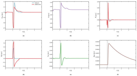
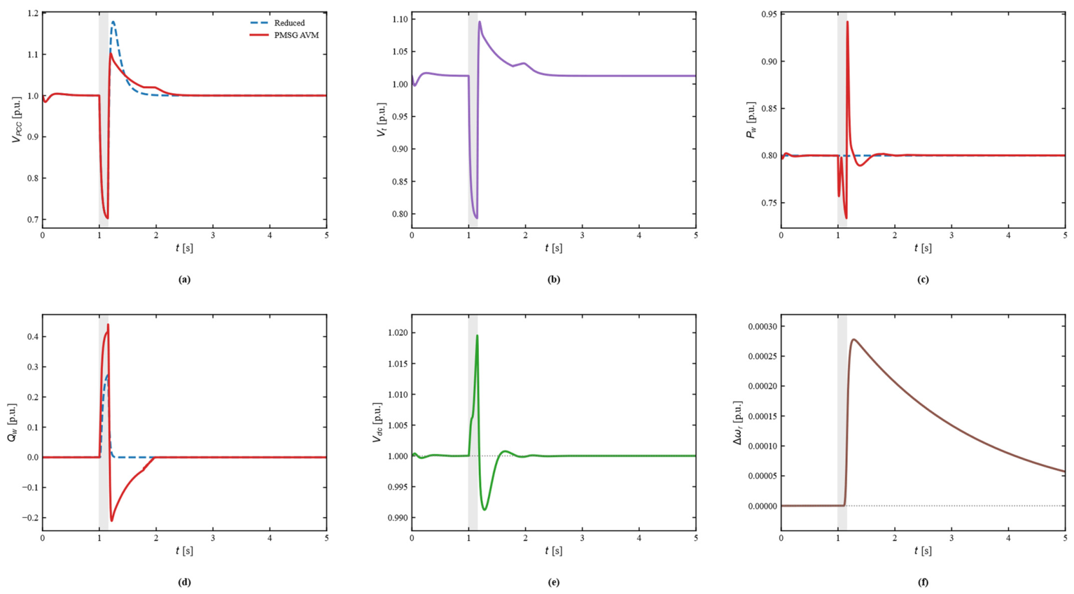
Figure 14 shows the representative SCR = 2.5 internal responses. In addition to PCC voltage, the higher-order model provides wind-turbine terminal voltage, active/reactive power, DC-link voltage, and rotor-speed deviation. The DC-link voltage remains approximately within 0.991–1.020 p.u. and the rotor-speed deviation remains small for the 0.15 s disturbance, whereas the grid-side reactive-power channel exhibits a post-clearance reverse adjustment that is absent from the reduced model. These internal states explain part of the reduced model’s overestimation of voltage overshoot.

Figure 14. Representative internal responses of the PMSG average-value model at SCR = 2.5. (a) PCC voltage. (b) Turbine terminal voltage. (c) Active power. (d) Reactive power. (e) DC-link voltage. (f) Rotor-speed deviation. Grey shading denotes the fault interval; dotted horizontal lines in the reactive-power and rotor-speed-deviation panels denote zero-reference levels.

Table 11 shows that the recovery-time difference between the reduced model and the PMSG average-value model remains only 1–2 ms across SCR = 1.5–10.0. At the same time, the PCC-voltage RMSE decreases monotonically from 0.0251 p.u. at SCR = 1.5 to 0.0028 p.u. at SCR = 10, and the post-fault maximum-voltage difference decreases from 0.1437 to 0.0096 p.u. The results indicate that the reduced model reproduces the recovery-time trend well, but its voltage-overshoot error is appreciably larger in very weak grids. This supports its use for planning-stage screening while reinforcing the need for a higher-fidelity model when overshoot magnitude and converter-level stresses are design-critical.

4.6.4. Balanced and Unbalanced Fault Responses

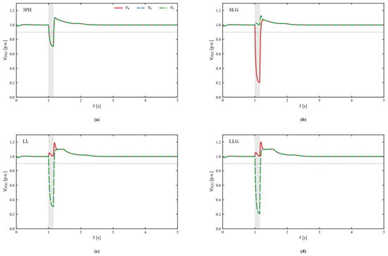
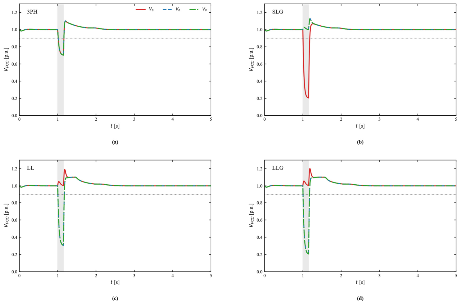
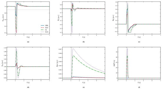
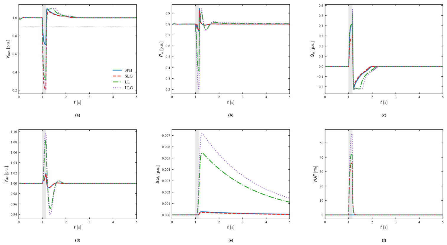
The sequence-domain model is used to compare a balanced three-phase disturbance with SLG, LL, and LLG retained-voltage patterns at SCR = 2.5 and Q_svg = 50 Mvar. Figure 15 confirms the expected phase-voltage asymmetry, while Figure 16 shows that unbalanced faults introduce additional negative-sequence, DC-link, and mechanical stress. The maximum voltage-unbalance factor increases from essentially zero for the balanced case to 36.1% for SLG, 43.3% for LL, and 56.4% for LLG. LL and LLG also produce the largest active-power reductions and DC-link overvoltages because negative-sequence suppression and positive-sequence voltage support consume converter-current margin.

Figure 15. PCC phase-voltage envelopes for balanced and unbalanced fault cases: (a) 3PH. (b) SLG. (c) LL. (d) LLG. The dotted horizontal line denotes the 0.9 p.u. voltage threshold, and grey shading denotes the fault interval.

Figure 16. Internal responses under balanced and unbalanced faults. (a) Minimum PCC phase voltage. (b) Wind-turbine active power. (c) Wind-turbine reactive power. (d) DC-link voltage. (e) Rotor-speed deviation. (f) Voltage-unbalance factor.Grey shading denotes the fault interval; dotted reference lines indicate the 0.9 p.u. voltage threshold or zero-deviation reference, as applicable.

Figure 15 illustrates the phase-voltage envelopes for the four fault patterns. Under the balanced three-phase (3PH) disturbance, the three phase-voltage trajectories remain coincident, as expected for a symmetrical event. In the SLG case, one phase is depressed to approximately 0.20 p.u. while the other two phases remain close to the prefault level, producing a pronounced phase-voltage asymmetry. For the LL case, two phases are depressed to approximately 0.30 p.u., whereas the remaining phase stays near its nominal level. The LLG case produces the deepest two-phase depression, with the two affected phases approaching 0.20 p.u. The post-clearance trajectories return toward the prefault operating point, but the unbalanced cases exhibit different overshoot and recovery patterns because the positive-, negative-, and zero-sequence components evolve differently. These results confirm that a single scalar PCC-voltage trajectory is insufficient to characterize asymmetric faults.

Figure 16 further compares the internal dynamic responses associated with the four fault types. The balanced 3PH case produces an essentially zero voltage-unbalance factor (VUF), whereas the maximum VUF reaches 36.1% for SLG, 43.3% for LL, and 56.4% for LLG. The LL and LLG cases also impose substantially greater converter and electromechanical stress: the minimum wind-turbine active power decreases to 0.369 and 0.197 p.u., respectively, while the maximum DC-link voltage rises to 1.083 and 1.096 p.u. and the maximum rotor-speed deviation increases to 0.00545 and 0.00715 p.u. In contrast, the 3PH and SLG cases show much smaller rotor-speed deviations and lower DC-link excursions under the adopted control settings. The recovery-time ordering is not identical to the ordering of VUF or internal stress; therefore, transient severity under unbalanced faults should not be assessed from T_rec alone. Table 12 summarizes these quantitative differences.

Table 12. Quantitative comparison of balanced and unbalanced fault responses.

Fault	Trec All Phase [s]	Vmin [p.u.]	VUFmax [%]	Pw,min [p.u.]	Vdc,max [p.u.]	|Delta Omega|max [p.u.]
3PH	0.012	0.703	0.0	0.734	1.020	0.00028
SLG	0.031	0.204	36.1	0.737	1.018	0.00022
LL	0.023	0.305	43.3	0.369	1.083	0.00545
LLG	0.025	0.205	56.4	0.197	1.096	0.00715

Table 12 quantitatively distinguishes voltage-recovery severity from internal converter and electromechanical stress. The balanced 3PH case has T_rec = 0.012 s, V_min = 0.703 p.u., and essentially zero VUF. The SLG case has the longest all-phase recovery time (0.031 s) and VUFmax = 36.1%, but its minimum active power, DC-link voltage, and rotor-speed deviation remain comparatively mild. By contrast, the LL and LLG cases produce much larger internal stress: Pw, min falls to 0.369 and 0.197 p.u., Vdc, max rises to 1.083 and 1.096 p.u., and the maximum rotor-speed deviation reaches 0.00545 and 0.00715 p.u., respectively. The LLG case also gives the largest VUFmax of 56.4%. Therefore, T_rec alone is insufficient to rank unbalanced-fault severity; phase-voltage unbalance, active-power depression, DC-link overvoltage, and rotor-speed deviation must be considered together.

The retained phase-voltage patterns used in this section are controlled study cases rather than fault-impedance solutions of a full three-phase network. The sequence-domain model captures RMS-envelope positive/negative/zero-sequence interactions and converter-current allocation, but it does not include switching harmonics, detailed transformer zero-sequence connections, or protection logic. Consequently, these results strengthen the comparative fault assessment but do not replace project-specific EMT fault studies.

5. Discussion

5.1. Comparison with Existing Studies

Grid-forming and virtual-synchronous-generator (VSG) control strategies provide a complementary perspective on coordinated voltage support in low-inertia systems [32,33]. Compared with the present grid-following SVG sizing framework, the cited VSG work focuses primarily on converter-control dynamics rather than SVG capacity planning; the two approaches are therefore complementary rather than directly competing.

Previous studies have approached weak-grid voltage support from complementary perspectives. Pushpak et al. [17] investigated STATCOM-based transient-stability enhancement for wind farms, whereas Taul et al. [18,19] emphasized converter synchronization and current-limiting dynamics during grid faults. Shah et al. [23] reviewed dynamic and transient converter modeling, and Sajadi et al. [25] discussed the dynamics and stability challenges associated with high shares of grid-following inverter-based resources. These works provide important insight into converter-level dynamics and fault behavior, while their primary focus is dynamic analysis or control rather than repeated SVG capacity sizing under simultaneous transient-performance, investment, and loss objectives.

In contrast to those dynamics-oriented studies, the present work places the transient simulation inside the capacity-optimization loop. Each candidate SVG rating is evaluated in the time domain, and post-fault recovery time is optimized simultaneously with investment cost and active-power loss under hard transient-voltage and stability constraints. The resulting Pareto set therefore quantifies the performance-cost-loss tradeoff directly. The observed diminishing marginal benefit of additional SVG capacity and the extension of the Pareto front toward longer recovery times and higher capacities under more severe faults provide planning-oriented information that is not available from a single controller or single-scenario transient study.

Methodologically, the contribution remains the coupling architecture between transient screening and multiobjective sizing rather than a new optimizer. The extended studies strengthen the robustness assessment in three complementary ways: the algorithm comparison tests optimizer dependence, the PMSG average-value model quantifies reduced-order model error, and the sequence-domain model reveals additional unbalanced-fault stresses. Nevertheless, none of these average-value models reproduces switching harmonics, detailed protection logic, transformer-specific zero-sequence paths, or site-specific fault impedances. Final equipment ratings should therefore still be verified with project-specific EMT/RTDS models or field disturbance data.

5.2. Applicability of Engineering Recommendations

The capacity values reported in this paper should be interpreted as planning-stage screening results on the adopted 100 MVA base rather than universal equipment ratings. Table 8 therefore reports traceable optimization/validation evidence instead of an arbitrary safety multiplier. For a project-specific design, the selected rating should be converted to the actual plant base and verified against credible balanced and unbalanced faults, converter-current limits, redundancy/N-1 requirements, the applicable grid code, and a higher-fidelity EMT or real-time digital model.

Two limitations remain. First, the higher-order PMSG model is an average-value model rather than a switching-level electromagnetic-transient model. Second, the wind farm is still represented by an aggregated plant equivalent rather than an explicit multi-machine collection-network model. Accordingly, final design verification should employ PSCAD/EMTDC, RTDS, or an equivalent detailed multi-machine model when project-level equipment ratings are determined.

6. Conclusions

This study proposes a multiobjective SVG sizing framework that embeds post-fault voltage-recovery dynamics in the capacity decision and then subjects the planning results to progressively richer validation models. The main conclusions are as follows:

Reduced-order sizing and grid-strength dependence. The RK4 screening model provides a computationally efficient optimization engine and yields a baseline knee-point solution of 18.5 Mvar at SCR = 2.5 and dFAULT = 0.80 p.u. Extending the grid-strength comparison to SCR = 7.5 and 10.0 confirms that the Q_svg-T_rec relationship retains a clear saturation region beyond the original weak-grid range; therefore, a fixed weak-grid sizing multiplier should not be extrapolated to normal or strong grids.

Optimizer robustness. Under the same population size, generation limit, constraints, and evaluation budget, NSGA-II and SMS-EMOA produce almost coincident Pareto fronts and very similar normalized HV/IGD+ values, whereas NSGA-III returns a sparser nondominated set for the present one-variable, three-objective problem. This indicates that the reported performance-cost-loss tradeoff is not an artifact of NSGA-II alone, while no claim of universal algorithm superiority is made.

Wind-turbine LVRT and coordinated control. Introducing reactive-current priority and converter-current limitation demonstrates that wind-turbine fault response can materially change the apparent SVG requirement. At SCR = 2.5 and dFAULT = 0.70 p.u., the refined coordinated-control scan reduces the SVG capacity required to meet T_rec <= 0.019 s from 39 to 13 Mvar under the adopted control parameters. This 66.7% reduction is a scenario-specific coordination potential rather than a universal derating factor.

Model-form validation and unbalanced faults. The ten-state PMSG average-value model predicts T_rec within 1–2 ms of the reduced model for SCR = 1.5–10.0 and gives very similar post-fault minimum voltage, but the reduced model increasingly overestimates voltage overshoot as the grid becomes weaker. The sequence-domain study further shows that SLG, LL, and LLG faults introduce substantial negative-sequence stress; in the adopted cases, VUF reaches 36.1%, 43.3%, and 56.4%, respectively, and LL/LLG produce the largest active-power reduction, DC-link rise, and rotor-speed deviation.

Engineering implication and limitation. Table 8 reports traceable optimization and validation results instead of applying an unsupported universal safety multiplier. The proposed workflow is suitable for narrowing the candidate SVG range, identifying tradeoff solutions, and assessing the value of coordinated wind-turbine support. However, the higher-order studies remain average-value/RMS-envelope models rather than switching-level EMT simulations. Final SVG ratings should therefore be converted to the actual plant base and verified against site-specific balanced/unbalanced faults, converter and protection limits, N-1 requirements, grid-code criteria, and detailed PSCAD/EMTDC, RTDS, or field-disturbance evidence.

References

- Blaabjerg, F.; Yang, Y.; Ma, K.; Wang, X. Power Electronics-The Key Technology for Renewable Energy System Integration. In Proceedings of the 2015 International Conference on Renewable Energy Research and Applications (ICRERA), Palermo, Italy, 22–25 November 2015; IEEE: Piscataway, NJ, USA, 2015; pp. 1618–1626. [Google Scholar]
- Afridi, S.K.; Koondhar, M.A.; Jamali, M.I.; Alaas, Z.M.; Alsharif, M.H.; Kim, M.-K.; Mahariq, I.; Touti, E.; Aoudia, M.; Ahmed, M.M.R. Winds of Progress: An In-Depth Exploration of Offshore, Floating, and Onshore Wind Turbines as Cornerstones for Sustainable Energy Generation and Environmental Stewardship. IEEE Access 2024, 12, 66147–66166. [Google Scholar] [CrossRef] [Scilit]
- Malik, F.H.; Khan, M.W.; Rahman, T.U.; Ehtisham, M.; Faheem, M.; Haider, Z.M.; Lehtonen, M. A Comprehensive Review on Voltage Stability in Wind-Integrated Power Systems. Energies 2024, 17, 644. [Google Scholar] [CrossRef] [Scilit]
- Gordon, S.; Hong, Q.; Bell, K. Implications of Reduced Fault Level and Its Relationship to System Strength: A Scotland Case Study. In Proceedings of the CIGRE Session 2022, Paris, France, 28 August–2 September 2022. Paper C4-10204. [Google Scholar]
- Sharma, P.; Gevorgian, V.; Shah, S.; Yan, W.; Alam, S.M.S.; Ojo, Y.; Vyakaranam, B.; Chuan, Q.; Liu, Y.; Liu, Y.; et al. Existing Methods for Grid Strength Assessment and Role of Hydropower in Future Grids; Technical Report NREL/TP-5D00-94961; National Renewable Energy Laboratory: Golden, CO, USA, 2025.
- Gong, H.; Wang, X.; Harnefors, L. Rethinking Current Controller Design for PLL-Synchronized VSCs in Weak Grids. IEEE Trans. Power Electron. 2022, 37, 1369–1381. [Google Scholar] [CrossRef] [Scilit]
- Taul, M.G.; Wu, C.; Chou, S.-F.; Blaabjerg, F. Optimal Controller Design for Transient Stability Enhancement of Grid-Following Converters Under Weak-Grid Conditions. IEEE Trans. Power Electron. 2021, 36, 10251–10264. [Google Scholar] [CrossRef] [Scilit]
- Taul, M.G.; Wang, X.; Davari, P.; Blaabjerg, F. An Overview of Assessment Methods for Synchronization Stability of Grid-Connected Converters under Severe Symmetrical Grid Faults. IEEE Trans. Power Electron. 2019, 34, 9655–9670. [Google Scholar] [CrossRef] [Scilit]
- He, X.; Geng, H. Transient Stability of Power Systems Integrated With Inverter-Based Generation. IEEE Trans. Power Syst. 2021, 36, 553–556. [Google Scholar] [CrossRef] [Scilit]
- Wang, X.; Taul, M.G.; Wu, H.; Liao, Y.; Blaabjerg, F.; Harnefors, L. Grid-Synchronization Stability of Converter-Based Resources-An Overview. IEEE Open J. Ind. Appl. 2020, 1, 115–134. [Google Scholar] [CrossRef] [Scilit]
- Wu, H.; Wang, X. Design-Oriented Transient Stability Analysis of PLL-Synchronized Voltage-Source Converters. IEEE Trans. Power Electron. 2020, 35, 3573–3589. [Google Scholar] [CrossRef] [Scilit]
- Yang, L.; Xu, Z.; Ostergaard, J.; Dong, Z.Y.; Wong, K.P. Advanced Control Strategy of DFIG Wind Turbines for Power System Fault Ride Through. IEEE Trans. Power Syst. 2012, 27, 713–722. [Google Scholar] [CrossRef] [Scilit]
- Jauch, C. Stability and Control of Wind Farms in Power Systems; Risoe-PhD-24(EN); Risoe National Laboratory: Roskilde, Denmark, 2006. [Google Scholar]
- Morgan, E.F.; Abdel-Rahim, O.; Megahed, T.F.; Suehiro, J.; Abdelkader, S.M. Fault Ride-Through Techniques for Permanent Magnet Synchronous Generator Wind Turbines (PMSG-WTGs): A Systematic Literature Review. Energies 2022, 15, 9116. [Google Scholar] [CrossRef] [Scilit]
- Moghadasi, A.; Sarwat, A.; Guerrero, J.M. A Comprehensive Review of Low-Voltage-Ride-Through Methods for Fixed-Speed Wind Power Generators. Renew. Sustain. Energy Rev. 2016, 55, 823–839. [Google Scholar] [CrossRef] [Scilit]
- Makolo, P.; Justo, J.J.; Mwasilu, F.; Zamora, R. Fault Ride Through Technique for DFIG-Based Wind Turbines Under Grid Three-Phase Faults. In Proceedings of the 2018 Australasian Universities Power Engineering Conference (AUPEC), Auckland, New Zealand, 27–30 November 2018. [Google Scholar]
- Pushpak, K.; Anuradha, B.K.; Ravi, A.; Abhishek, A. Improving Transient Stability of Wind Farm Using FACTS Devices Focused on STATCOM. Int. J. Eng. Appl. Sci. Technol. 2016, 1, 163–167. [Google Scholar]
- Taul, M.G.; Golestan, S.; Wang, X.; Davari, P.; Blaabjerg, F. Modeling of Converter Synchronization Stability Under Grid Faults: The General Case. IEEE J. Emerg. Sel. Top. Power Electron. 2022, 10, 2790–2804. [Google Scholar] [CrossRef] [Scilit]
- Taul, M.G.; Wang, X.; Davari, P.; Blaabjerg, F. Current Limiting Control With Enhanced Dynamics of Grid-Forming Converters During Fault Conditions. IEEE J. Emerg. Sel. Top. Power Electron. 2020, 8, 1062–1073. [Google Scholar] [CrossRef] [Scilit]
- Tsili, M.; Papathanassiou, S. A Review of Grid Code Technical Requirements for Wind Farms. IET Renew. Power Gener. 2009, 3, 308–332. [Google Scholar] [CrossRef] [Scilit]
- Li, H.; Wang, C.; Tian, H.; Ren, Z.; Zhao, E.; Xu, L. A Multi-Objective Optimization Planning Framework for Active Distribution System via Reinforcement Learning. Distrib. Gener. Altern. Energy J. 2023, 38, 1741–1762. [Google Scholar] [CrossRef] [Scilit]
- Manasa, D.; Gopi Siva Prasad, M.; Jayakrishna, G. STATCOM Control under Asymmetrical Grid Faults at FSIG-Based Wind Farms. Int. J. Electr. Electron. Res. 2014, 2, 124–132. [Google Scholar]
- Shah, C.; Vasquez-Plaza, J.D.; Campo-Ossa, D.D.; Patarroyo-Montenegro, J.F.; Guruwacharya, N.; Bhujel, N.; Trevizan, R.D.; Rengifo, F.A.; Shirazi, M.; Tonkoski, R.; et al. Review of Dynamic and Transient Modeling of Power Electronic Converters for Converter Dominated Power Systems. IEEE Access 2021, 9, 82094–82117. [Google Scholar] [CrossRef] [Scilit]
- Emmerich, M.T.M.; Deutz, A.H. A Tutorial on Multiobjective Optimization: Fundamentals and Evolutionary Methods. Nat. Comput. 2018, 17, 585–609. [Google Scholar] [CrossRef] [Scilit] [PubMed]
- Sajadi, A.; Ranola, J.A.; Kenyon, R.W.; Hodge, B.-M.; Mather, B. Dynamics and Stability of Power Systems With High Shares of Grid-Following Inverter-Based Resources: A Tutorial. IEEE Access 2023, 11, 29591–29613. [Google Scholar] [CrossRef] [Scilit]
- Blank, J.; Deb, K. pymoo: Multi-Objective Optimization in Python. IEEE Access 2020, 8, 89497–89509. [Google Scholar] [CrossRef] [Scilit]
- Deb, K.; Pratap, A.; Agarwal, S.; Meyarivan, T. A Fast and Elitist Multiobjective Genetic Algorithm: NSGA-II. IEEE Trans. Evol. Comput. 2002, 6, 182–197. [Google Scholar] [CrossRef] [Scilit]
- Qiu, Z.; Gu, Y. Power Margin Ratio-A Large-Signal System Strength Metric for Inverter-Based Resources-Dominated Power Systems. arXiv 2026, arXiv:2602.11429. [Google Scholar]
- Zitzler, E.; Thiele, L. Multiobjective Evolutionary Algorithms: A Comparative Case Study and the Strength Pareto Approach. IEEE Trans. Evol. Comput. 1999, 3, 257–271. [Google Scholar] [CrossRef] [Scilit]
- Zitzler, E.; Thiele, L.; Laumanns, M.; Fonseca, C.M.; da Fonseca, V.G. Performance Assessment of Multiobjective Optimizers: An Analysis and Review. IEEE Trans. Evol. Comput. 2003, 7, 117–132. [Google Scholar] [CrossRef] [Scilit]
- GB/T 19963.1-2021; Technical Specification for Connecting Wind Farm to Power System—Part 1: On Shore Wind Power. State Administration for Market Regulation. Standardization Administration of China: Beijing, China, 2021.
- Rosso, R.; Wang, X.; Liserre, M.; Lu, X.; Engelken, S. Grid-Forming Converters: Control Approaches, Grid-Synchronization, and Future Trends-A Review. IEEE Open J. Ind. Appl. 2021, 2, 93–109. [Google Scholar] [CrossRef] [Scilit]
- Li, F.; Liu, Y.; Liu, Y. Macroscopic State-Based Reactive Voltage Control of Virtual Synchronous Generator in AC Microgrid. Int. J. Circuit Theory Appl. 2025, 53, 2214–2226. [Google Scholar] [CrossRef] [Scilit]
Disclaimer/Publisher’s Note: The statements, opinions and data contained in all publications are solely those of the individual author(s) and contributor(s) and not of MDPI and/or the editor(s). MDPI and/or the editor(s) disclaim responsibility for any injury to people or property resulting from any ideas, methods, instructions or products referred to in the content. |
© 2026 by the authors. Licensee MDPI, Basel, Switzerland. This article is an open access article distributed under the terms and conditions of the Creative Commons Attribution (CC BY) license.