


Abstract
As wind and photovoltaic (PV) generation expands, power systems increasingly need coordinated forecasts for multiple sites. Sites share weather influences but respond differently, so a forecasting model must learn common temporal patterns while preserving differences between energy types and individual sites. We propose a method based on shared multiscale representations. A bidirectional gated recurrent unit (BiGRU) extracts historical features. We combine daily variation with recent fluctuations, then use direction-specific information exchange and site-specific heads to produce coordinated predictions. An energy-balanced objective coordinates training across wind and PV tasks. We evaluate the method using simulated power series generated from the fifth-generation atmospheric reanalysis (ERA5) of the European Centre for Medium-Range Weather Forecasts at the geographic coordinates of seven wind and PV sites in the Wujiang region. Rolling annual evaluations show lower mean absolute error than the tested graph and Transformer baselines in every test year under common experimental settings. Component comparisons in a compact model support retaining fine temporal resolution for recent changes. A separate analysis finds that within-energy dependence modeling reduces Brier scores for simultaneous low-output events. These results support shared temporal modeling for coordinated multisite wind–PV forecasting and provide simulation evidence for regional joint-output analysis.
1. Introduction
Coordinated forecasts for wind and photovoltaic (PV) sites support regional energy scheduling, reserve allocation and market participation. Wind and PV respond to different physical drivers and have distinct diurnal patterns and fluctuations. Sites in the same region also experience common weather processes, which create relationships among their outputs. Regional forecasting needs to describe local site behavior while using information across sites and energy types. A systematic review describes the expansion of wind–PV forecasting from centralized models to collaborative approaches such as federated learning; model applicability and consistency of comparisons across sites remain open questions [1]. Renewable forecasting and trading competitions show why portfolio output and its uncertainty matter alongside individual-site errors [2,3].
Deep learning studies of wind–PV forecasting use temporal features, spatial relationships and multitask learning. Hybrid recurrent and Transformer architectures combine different temporal modeling mechanisms and have been applied to wind and PV power prediction [4]. In multisite PV forecasting, multigraph attention and graph attention networks represent intersite links and combine them with heterogeneous inputs [5,6]. For mixed wind–PV systems, heterogeneous graph models jointly represent dependencies across sites and energy types [7], while multitask bidirectional long short-term memory (BiLSTM) combined with a graph convolutional network (GCN)–Transformer integrates individual prediction and cluster correction for day-ahead wind–solar forecasting [8]. Complementary-resource aggregation, physics-informed modeling, scenario generation and probabilistic forecasting describe other aspects of regional output [9,10,11,12]. Multitask learning uses shared representations to exploit relationships among prediction tasks [13], including attention-based regional wind–PV forecasting [14] and wind–solar–load models that combine shared and task-specific features [15].
Recent studies also examine which information to use and how to interpret and train the models. Spatiotemporal attention extracts temporal and spatial information relevant to wind and PV output [16]; interpretable stacking has been applied to PV prediction and fault analysis [17]. Research on distributionally robust scheduling and energy–carbon optimization in energy hubs connects forecasting information with operating constraints and decision objectives [18,19]. Adaptive loss balancing and gradient projection address coordination between tasks during training [20,21]. Across these approaches, a model must use common patterns of variation while retaining the different responses of energy types and sites.
Two issues require closer examination: the temporal scales retained by the model and the way information is shared. Wind and PV outputs contain slow changes, including daily cycles, as well as rapid fluctuations associated with recent weather disturbances. These scales can contribute differently to a forecast. Shared representations need to capture common site behavior while allowing for differences between wind and PV and between individual sites. Evaluating multiscale representations and cross-energy information exchange therefore requires consistent data and training conditions, together with component comparisons. Regional operation also depends on whether wind and PV output can be low at the same time. Point-forecast errors alone cannot answer that question; joint-event assessment requires predictive distributions and their dependence structure [22,23]. Joint-low-output analysis complements the information obtained from coordinated point forecasts.
We study coordinated multisite wind–PV forecasting with shared multiscale representations. A shared bidirectional gated recurrent unit extracts historical features that combine daily variation with recent changes. Energy-specific information exchange and site-specific prediction heads then produce multisite outputs. We evaluate the method through rolling annual comparisons and component controls using weather-driven power simulations at seven sites in the Wujiang region. A separate joint-low-output analysis examines simultaneous low-output events. The study offers a testable method for coordinated forecasting and simulation evidence for later joint-output assessments that incorporate scheduling and reserve requirements.
2. Materials and Methods
2.1. Data and Proxy Construction
The fixed WGS84 coordinates in Table 1 identify seven outputs and their weather-extraction locations in the Wujiang region. They are not equipment footprints or measured power records. The fifth-generation atmospheric reanalysis (ERA5) from the European Centre for Medium-Range Weather Forecasts (ECMWF) [24,25] supplies 2021–2025 inputs; its approximately 31 km atmospheric resolution and delivered 0.25° grid do not resolve plant-scale terrain. W-2 is a project-map anchor with approximately 15 km positional uncertainty. The simulation uses all four PV and three wind outputs with the original conversion settings; the coordinate uncertainty remains part of the study definition.
Table 1.
Coordinate anchors and output identities. W-2 has approximately 15 km positional uncertainty; capacities and operating records of the named plants are not inferred from these points.
PV targets use a common 1.0 MW AC and 1.2 MWp DC reference, 25° tilt, 180° azimuth and 0.20 albedo. Solar geometry, cloud-partitioned irradiance and isotropic sky/ground reflection determine plane-of-array irradiance. A Faiman-type temperature correction uses U0 = 25.0, U1 = 6.84 and a −0.0047 °C−1 power coefficient; system loss is 0.14 and inverter efficiency is 0.96. AC power is clipped to [0, 1.0] MW and normalized. Nighttime geometry or nonpositive irradiance yields zero simulated PV. Wind targets use 100 m input wind, a 90 m hub, exponent 0.143, reference density 1.225 kg m−3, and a cubic curve from 3.0 to 11.4 m s−1, with rated output below 25.0 m s−1 and cut-out/restart at 25.0 m s−1.
The hourly tensor contains 14 weather variables per station: temperature, dewpoint, relative humidity, surface pressure, 10 m wind speed/direction, precipitation, the retained surface-shortwave series, single-level total/direct shortwave, 100 m wind speed/direction, cloud cover and surface roughness. The fixed input manifests identify each series and how accumulated values are handled. The two source archives overlap for 168 h. We check that their weather and power values match exactly before removing duplicate records. The combined time axis contains 43,824 h. Power stays in [0, 1] per unit (p.u.). Measured supervisory control and data acquisition (SCADA), outage, curtailment, maintenance and sensor-error series are unavailable, which prevents estimation of proxy-to-measured error.
2.2. Forecasting Tasks and Rolling Folds
Each task predicts seven powers at target time t from a nominal origin o = t − h, where h is 3, 6, 12 or 24 h. Origins occur at 00:00, 06:00, 12:00 and 18:00 UTC. The 168 h history is [o − 168 h, o). Historical weather context uses the latest record with the target’s UTC clock hour that satisfies a nominal one-hour availability delay. Thus, its timestamp is t − 24 h for the 3/6/12 h tasks and t − 48 h for the 24 h task. These records fall within the historical window. The extra context token provides another representation of information already available to the model, without introducing a new observing system or future ERA5 values.
The one-hour rule is an imposed timestamp convention within reanalysis data, not a claim about ERA5’s real-time release latency. Known calendar inputs are target-hour sine/cosine, annual-phase sine/cosine using 365.2425 days, and h/24. Station metadata indicates PV or wind. BiGRU traverses only the available historical sequence in both directions; its backward pass does not read future targets. Weather is standardized separately for each station and variable using the union of hourly records actually consumed by training histories in that fold. Means and population standard deviations are fitted in float64 and stored in float32; a standard deviation below 10−6 would use divisor 1 with its coordinate recorded.
We assign targets to calendar partitions before constructing windows. For each test year, the preceding year supplies validation and earlier years from 2021 supply expanding training data (Table 2). Training and validation targets stop 24 h before the next partition begins. Test targets cover the complete calendar year, including valid early-year tasks whose origins fall in the previous year. The first training week lacks sufficient historical coverage and is excluded. Constructing tasks from the hourly axis includes seven boundary tasks omitted by the earlier origin-first partition.
Table 2.
Expanding rolling folds and task counts. Training and validation have a 24 h target embargo at their right boundary; all test years are retrospective.
2.3. Shared Multiscale B2 Architecture
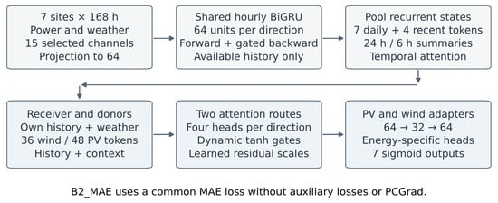
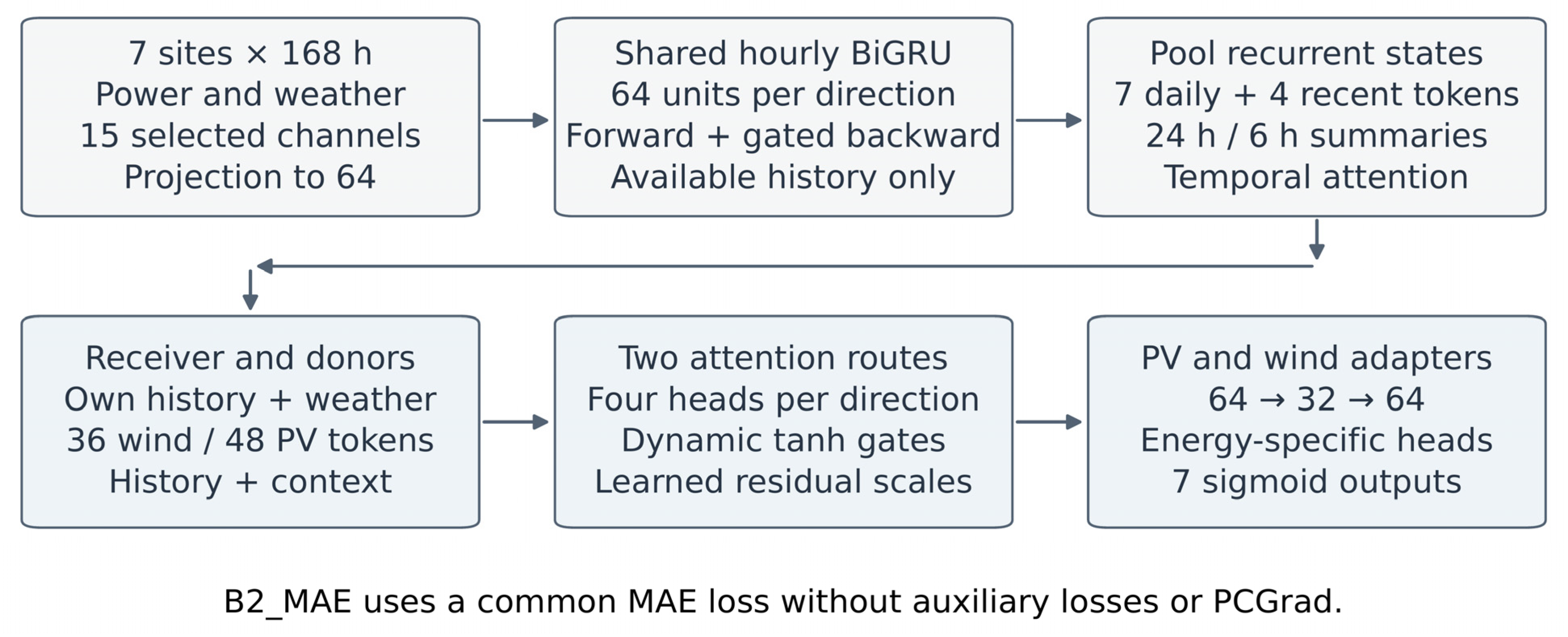
B2 processes each station’s 168 hourly records before temporal pooling (Figure 1). The 15 input channels comprise power and 14 weather variables. A context-conditioned selector, using the five calendar/horizon features and two energy indicators, multiplies the channels by feature-count-scaled softmax weights. Its final layer is initialized to zero, making selection initially an identity mapping. Selected inputs are projected from 15 to 64 dimensions with layer normalization (LayerNorm) and a Gaussian error linear unit (GELU). One shared, single-layer BiGRU [26], with 64 units per direction, encodes all stations. At each historical position, forward and backward states are fused as forward + tanh(r) ⊙ backward, where the 64-dimensional parameter r starts at zero. Both passes remain entirely inside the available history.
Figure 1.
B2 forecasting architecture trained with the common mean absolute error (MAE) objective. Multiscale pooling follows hourly shared recurrence. The two cross-energy attention routes have separate parameters. The tanh gate is an internal signed message multiplier, and all weather inputs obey Section 2.2. Arrows denote computational information flow. BiGRU, bidirectional gated recurrent unit; PV, photovoltaic; PCGrad, projecting conflicting gradients.
The fused hourly sequence is averaged into seven nonoverlapping 24 h tokens over the week and four nonoverlapping 6 h tokens over the latest day. Thus, B2 retains 11 post-recurrence tokens per station. Station and token-position embeddings distinguish their identities. Four-head temporal attention uses station identity and the target calendar/horizon embedding as its query; a learned residual scale, initialized at 0.10, adds the pooled result to the fused directional final states. The resulting 64-dimensional history summary is combined with energy metadata (8 dimensions), calendar features (8) and selected same-clock historical weather (16), then projected from 96 to 64 dimensions. This context-bearing representation supplies both the receiver query and the additional donor token.
Each PV receiver attends to 36 wind donor tokens (three stations × 12 tokens), and each wind receiver to 48 PV donor tokens (four × 12). Eleven tokens per donor encode multiscale history; the twelfth is its context-bearing representation. For direction d, receiver query qs, donor memory Md and target embedding h, the four-head attention message and gated residual update are given in Equation (1).
Here, MHA denotes multi-head attention and ∥ concatenation. The learned scalar ρd sets the direction scale; Wd and bd parameterize the scalar gate γd,s applied to the attention message. The two directions use separate attention and linear gate parameters, with direction scales initialized at 0.05 and dropout probability 0.10. Energy-specific residual adapters (64 → 32 → 64) and linear heads produce seven sigmoid-bounded outputs. B2 has 124,764 trainable parameters. The sign of γ can reverse an entire latent update, whose entries can themselves have either sign; it is neither a station-pair correlation nor a physical transfer coefficient. We evaluate the contribution of this computation through the controls described below. B2_MAE uses this inference architecture with the common mean absolute error (MAE) objective. The historical B2 experiments used auxiliary penalties, adaptive weighting and projecting conflicting gradients (PCGrad).
2.4. Comparisons and Component Series
A0–A6 form a separate simplified architecture series (Table 3), with d = 32 and 16 recurrent units per direction. Unlike B2, A0 averages power before recurrence into seven daily and four recent 6 h blocks; weather enters local context rather than the recurrent history tokens. The same BiGRU is reused across both scale sequences. A single shared, bias-free, four-head attention module combines receiver queries with donor power-history tokens and optional donor-context tokens. The latter bundle donor weather summaries, same-clock history, identity and known-time features. Non-affine LayerNorm normalizes messages and readout inputs; a multilayer perceptron (MLP) sigmoid gate scales the residual message before energy-specific sigmoid point heads. These changes jointly alter capacity, feature access and computation relative to B2.
Table 3.
Complete model architectures and conditional interventions within A0. B2_MAE is the main forecasting model. A1–A6 are comparisons within A0, not single-module B2 ablations. All ten implementations use the same available raw inputs, seven outputs and training rules.
A1 retains all seven daily means and the same 168 h historical coverage, removing only the additional recent resolution. A2 removes the full extra donor-context token while retaining donor power histories and receiver-local weather. Its gate has no separate donor-weather input. This intervention tests the additional donor-context token as a whole, including weather, donor identity, known-time features and their fusion; it cannot isolate the weather contribution. Shared calendar/horizon information remains available locally. Input-derivative and perturbation checks verify these access boundaries.
A3 replaces the dynamic MLP gate with 28 learned sigmoid constants, one per receiving station and horizon; A4 fixes every gate to 1. A6 combines A2’s context removal with A3’s constants. Message normalization removes a direct affine rescaling at that location, but other trainable projections and the readout can still compensate for constant scaling. The A3/A4 contrast therefore concerns statistical parameterization and optimization, not an identified physical transfer coefficient. A0/A2/A3/A6 form the complete context-present/absent by dynamic/constant-gate design.
A5 routes attention to the receiver’s own energy group, including itself. It uses exactly the same parameter names, shapes and count as A0, with every module active. Perturbing the other energy’s power, weather and metadata leaves its receiver outputs and gates unchanged, and the corresponding input Jacobians are zero. Because the encoder and attention parameters are still trained jointly, A5 permits training transfer through shared parameters. It is a control for cross-energy forward message passing, not independently trained energy models. Its analytic operation count differs slightly because 42 + 32 differs from 2 × 4 × 3.
We adapt MTGNN [27] and PatchTST [28] as external baselines. They receive the same raw power, weather, calendar and energy inputs, but their representation differs: MTGNN pools 168 h to 12 positions, whereas PatchTST projects 15 power/weather channels and uses 24 h patches with stride 12 h. Both retain the contextual readout with non-affine normalization. Both reference implementations are adapted to this task and trained under the shared finite budget; we do not exhaustively tune either model family. The accompanying data provide parameter counts and training histories; Section 3.4 summarizes the measured computational costs.
Every fit minimizes one half of PV MAE plus one half of wind MAE. AdamW uses learning rate 0.001, weight decay 0.0001, batch size 128 and gradient-norm clipping at 1.0. There are no auxiliary penalties, adaptive task weights, gradient projection or learning-rate scheduler. Training runs for at least 10 and at most 50 epochs, with patience 10 and significant-improvement threshold 10−5 on validation MAE. Any strict validation improvement saves a checkpoint, while the patience counter resets only after the declared significant improvement. Validation selects the checkpoint independently for every fit; epochs are not selected from test performance.
Seeds 2026091101, 2026091102 and 2026091103 are fixed across all models and years. The same epoch-specific task permutation is used for each paired seed and fold. Same-name, same-shape common parameters in A1–A6 are copied from that seed’s canonical A0 initialization, excluding gate-specific tensors, and the random number generator (RNG) is reset after construction. This design gives 90 fits. Before fixing the protocol, we ran ten updates per model on training data to check finite losses and gradients, module activity and runtime. This check did not use validation or test errors. All 90 selected checkpoints were fixed before computing test predictions. CUDA seeds and deterministic preferences are recorded, including unsupported-kernel warnings; bitwise retraining identity is not assumed.
2.5. Evaluation and Uncertainty
We use an energy-balanced version of mean absolute error (MAE) as the primary metric; MAE is a standard measure of forecast accuracy [29]. It gives equal weight to PV and wind rather than to all seven stations pooled together. The energy-balanced metric is defined in Equation (2). The secondary energy-balanced root-mean-square error (RMSE) first pools squared errors within each energy group, takes each group’s square root, then averages the two roots. Results report the mean and sample standard deviation of scores from the three separate fits, not the score of their averaged prediction. Complete annual, seasonal, 3/6/12/24 h, energy-group and station decompositions are retained; seeds and horizons are not independent geographic or climatic replications. Scores are rounded only for presentation; contrasts and intervals are calculated from unrounded values. The index e denotes either the PV group or the wind group, and ys and ŷs denote the target and prediction for station s.
Every contrast is reported with its subtraction order. Comparator minus B2_MAE is positive when B2_MAE is more accurate; Aj minus A0 is positive when removing or changing that A0 component is harmful. The context-by-gate interaction is defined in Equation (3). It asks whether the additional context benefit is larger with a dynamic gate than with learned constants. A6’s rank alone cannot establish interaction. We computed the B2-versus-external contrasts post hoc from the same fixed paired bootstrap draws, without additional fitting or test-based tuning.
For temporal uncertainty, we first average the three fitted models’ losses at each task and aggregate by UTC target day. We then draw 5000 paired, non-circular moving-block resamples of seven target days using seed 2026091199. All horizons and stations for a sampled day move together, and task counts determine weights. Each year’s 95% percentile interval is reported separately. The equal-weight average over the three annual metrics is descriptive. The intervals condition on fitted models and observed years; they omit refitting uncertainty, are not multiplicity-adjusted and do not establish population-wide generalization.
Point-series covariance and correlation errors are reported separately by horizon and by within-PV, within-wind and cross-energy pairs. These errors measure co-variation in the predicted and target time series and do not measure conditional covariance in residual scenarios. Gate values are summarized by station and horizon, and by weather strata defined from training data. Neither a variable internal gate nor improved point-series covariance establishes calibrated joint probabilities. The study below evaluates joint-low-output probabilities separately. Training and the main ranking use no composite score that mixes units.
2.6. Fixed Marginal Joint Risk Study
The joint-risk analysis uses the earlier five-seed B2/Diag study. Its fitted models are separate from the current B2_MAE models. Saved point predictions and positive diagonal conditional standard deviations determine the station scenarios. The four dependence arms have identical finite empirical station marginals: Diag, WithinEnergy, StaticCrossGate and ContextCrossGate. WithinEnergy restores within-PV and within-wind dependence. The two cross-gate arms preserve the complete PV and wind group scenario sets from WithinEnergy and change only their row pairing. This design separates any added cross-energy benefit from within-energy dependence. The point predictions remain fixed; point MAE and RMSE cannot improve in this experiment.
Dependence templates and gate calibration use separate halves of 2024, with label-availability checks at the boundary; 2025 supplies 5833 archived evaluation rows. The template uses shrunk normal-score residual correlations. A bounded analytic cross-block gate preserves positive definiteness; 512 fixed Sobol scenarios, station-wise rank matching and whole-group assignment preserve the finite marginals. Static and contextual gates are selected on a fixed nine-value grid using calibration-period Brier loss. The contextual states combine four horizons and two predicted levels for each energy group. Fitting applies to scheduled daytime (08:00 ≤ Beijing target clock < 18:00), because that is the archived variance head’s support; all other rows retain identical Diag scenarios. Finite sampling, clipping and assignment do not guarantee empirical covariance equal to the analytic matrix or monotonic event probabilities in the gate.
The primary event requires both equal-weight energy-group means to be strictly below 0.10 p.u.; it is an illustrative low-output event, not a validated reserve or outage threshold. Its estimated probability is the fraction of joint scenarios satisfying that event, and the Brier score is defined in Equation (4). Here, z is the joint-event indicator, p is its predicted probability, and BS denotes the Brier score.
We report daytime and all-time results, 0.20-threshold sensitivity, probability bias and the cross-energy variogram score (exponent 0.5) [23]. For this earlier dependence study, temporal intervals use 2000 circular moving-block resamples of seven and 28 origin days and condition on five saved fits. We analyze the two studies separately because their task axes, training procedures and uncertainty methods differ. The fixed 0.75 p.u. joint-high-output event in this archived dependence study has no positive cases and cannot validate high-event detection; it differs from the original training-quantile diagnostic.
3. Results
3.1. Overall Point Forecasting Performance
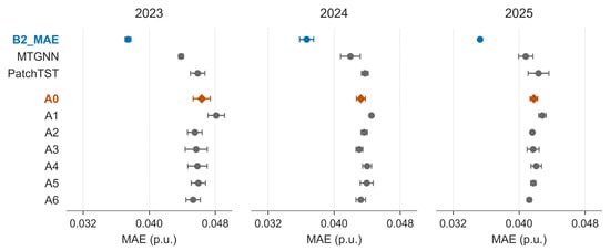
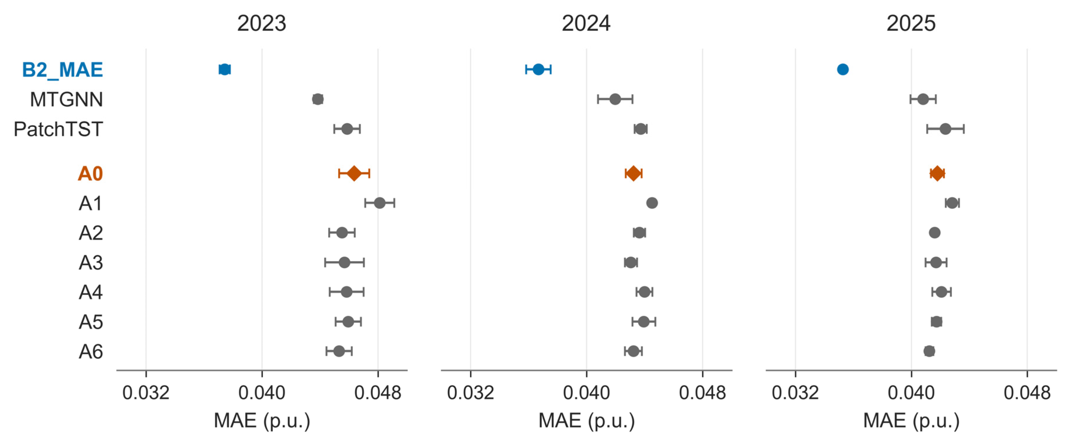
B2_MAE has the lowest mean energy-balanced MAE among all ten implementations in each complete test year (Figure 2). Its 2023/2024/2025 values are 0.037430/0.036668/0.035266 p.u., compared with 0.046360/0.043233/0.041790 for A0. Relative to A0, the reductions are 19.26%, 15.18% and 15.61%, with paired temporal intervals excluding zero in every year. The balanced RMSEs also favor B2_MAE: 0.090306/0.087154/0.081219 versus 0.108580/0.100676/0.094568 for A0. These are averages of separately fitted model scores, with seed dispersion retained.
Figure 2.
Annual energy-balanced MAE for all ten implementations. Points show mean MAE across three fitted models; horizontal bars show the sample standard deviation (SD) of their scores. Each year is a separate rolling evaluation with separately fitted models. Complete numerical values are provided in Supplementary Data S1. Values are expressed in per unit (p.u.).
Against adapted MTGNN, B2_MAE reduces mean MAE by 14.66%, 12.62% and 13.58%; against adapted PatchTST the reductions are 18.39%, 16.14% and 16.71%. The corresponding post hoc paired intervals exclude zero in all three years (Supplementary Data S1). MTGNN outperforms A0 in annual means throughout, whereas PatchTST’s comparison with A0 changes direction. These comparisons include every tested model and apply to the specific implementations and training budget used here. They do not establish superiority across the MTGNN or PatchTST model families.
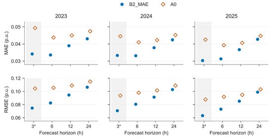
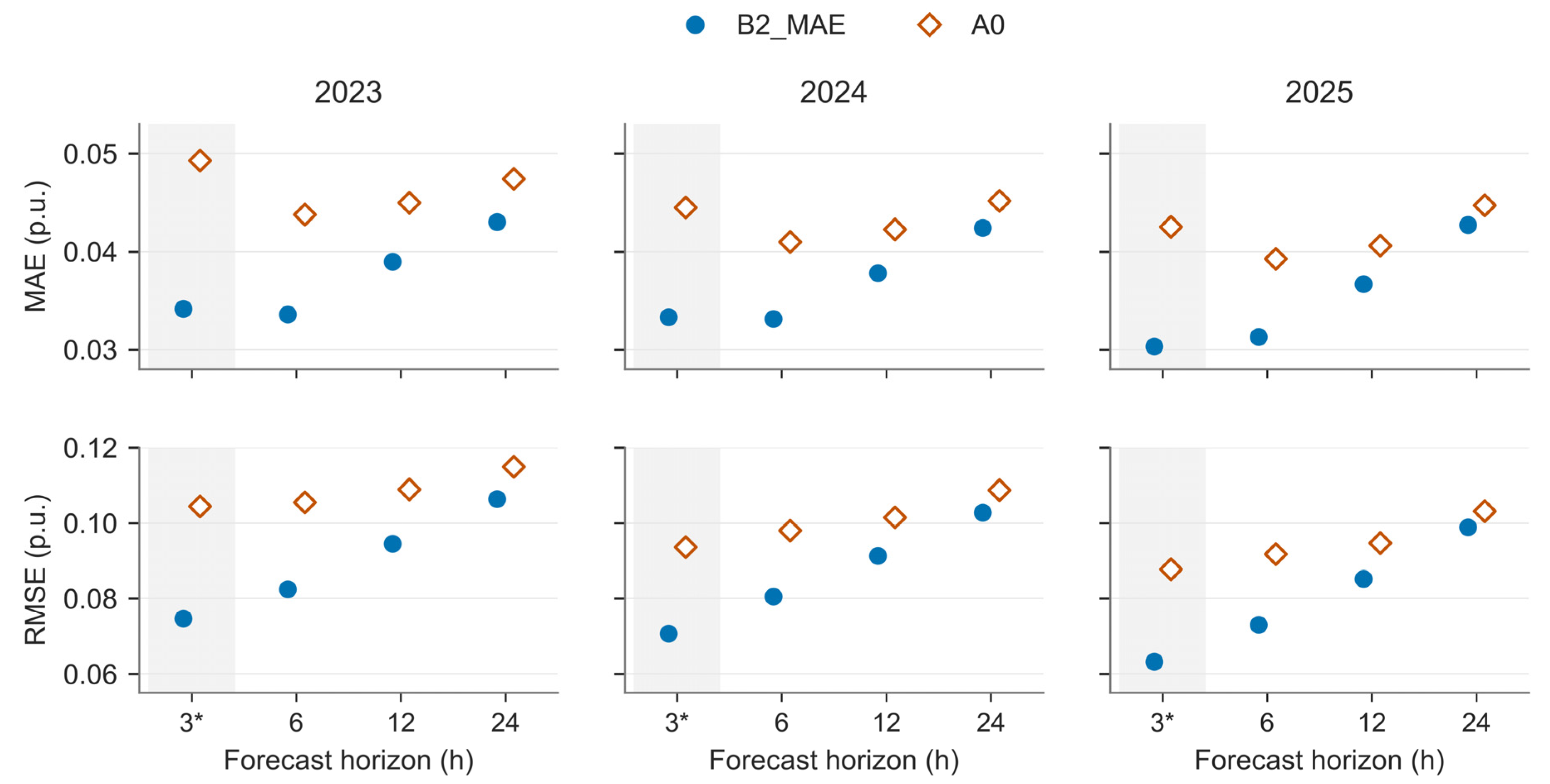
B2_MAE has lower mean MAE than A0 in all twelve combinations of test year and horizon, for energy-balanced, PV and wind errors. Figure 3 shows balanced MAE and RMSE for both models. In 2025, B2_MAE’s balanced MAE is 0.030340, 0.031318, 0.036690 and 0.042714 p.u. at 3, 6, 12 and 24 h, respectively. Comparisons across horizons also depend on the target time. With fixed forecast origins, the 3 h tasks target 03:00/09:00/15:00/21:00 UTC, while the 6/12/24 h tasks target 00:00/06:00/12:00/18:00 UTC. Nonmonotonic errors can therefore reflect both lead time and the times of day being predicted.
Figure 3.
Energy-balanced MAE (top) and root-mean-square error (RMSE; bottom) for B2_MAE and A0 by test year and forecast horizon. Points show mean scores across three fitted models. The shaded 3 h columns, marked with an asterisk, correspond to target times 03:00/09:00/15:00/21:00 UTC; the other horizons target 00:00/06:00/12:00/18:00 UTC. Horizons are shown as discrete categories because comparisons also depend on target-clock composition. Complete numerical values are provided in Supplementary Data S1.
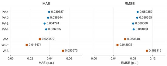
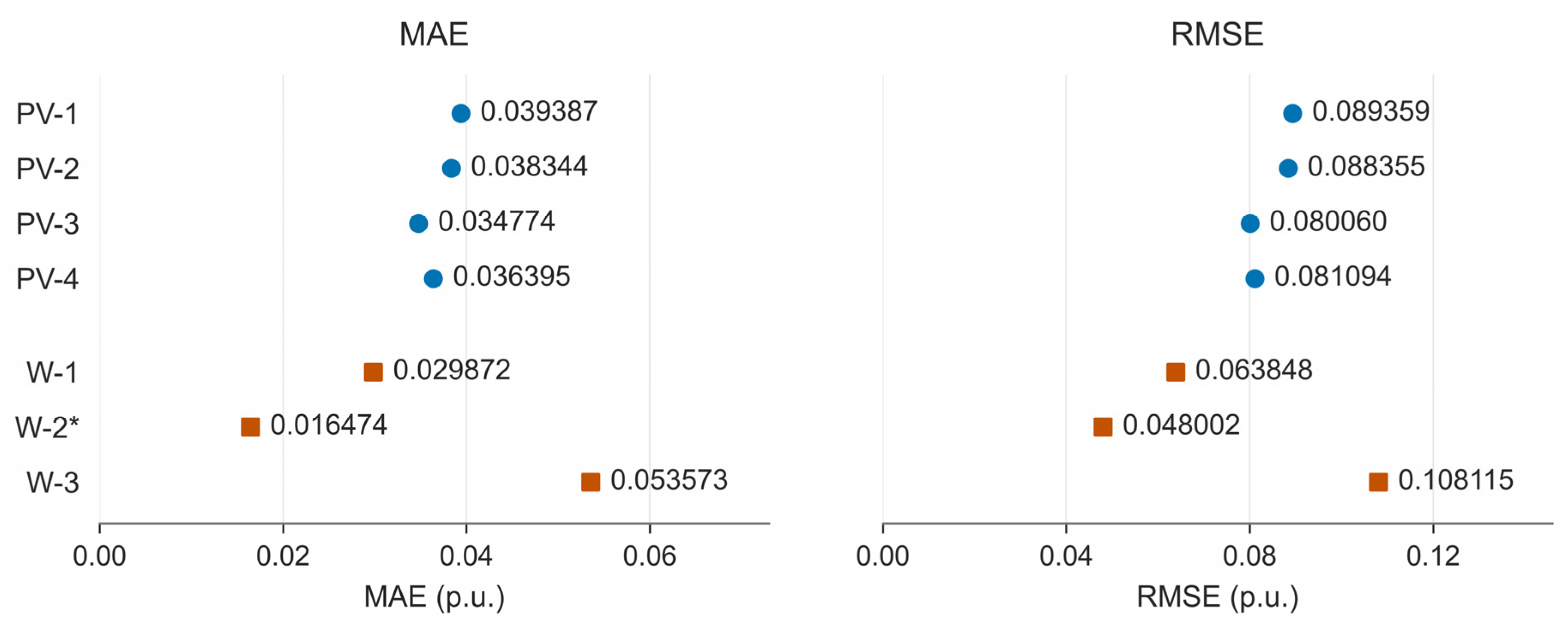
Across the seven simulated outputs in 2025, B2_MAE’s station MAE ranges from 0.016474 p.u. at W-2 to 0.053573 p.u. at W-3. The four PV values range from 0.034774 to 0.039387 p.u. Figure 4 shows each station’s MAE and RMSE. W-2’s lower error does not resolve its coordinate uncertainty or establish measured-plant accuracy. The accompanying data retain complete seasonal and station results for every model, year and horizon.
Figure 4.
B2_MAE station-level mean absolute error (MAE) and root-mean-square error (RMSE) in 2025, averaged across the scores of three fitted models. Labels give the numerical values. Blue circles denote photovoltaic (PV) outputs, and orange squares denote wind outputs. Station labels follow Table 1; all results refer to simulated power. The asterisk identifies W-2, whose coordinate has approximately 15 km positional uncertainty. Complete numerical values are provided in Supplementary Data S1.
3.2. Evidence for the Tested Components
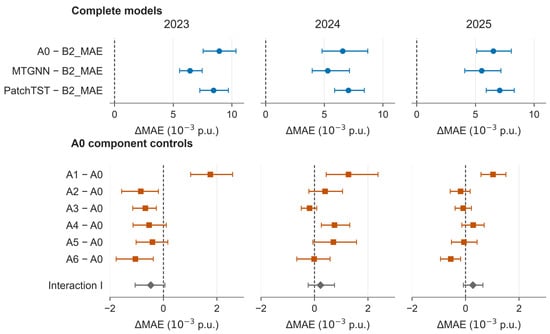
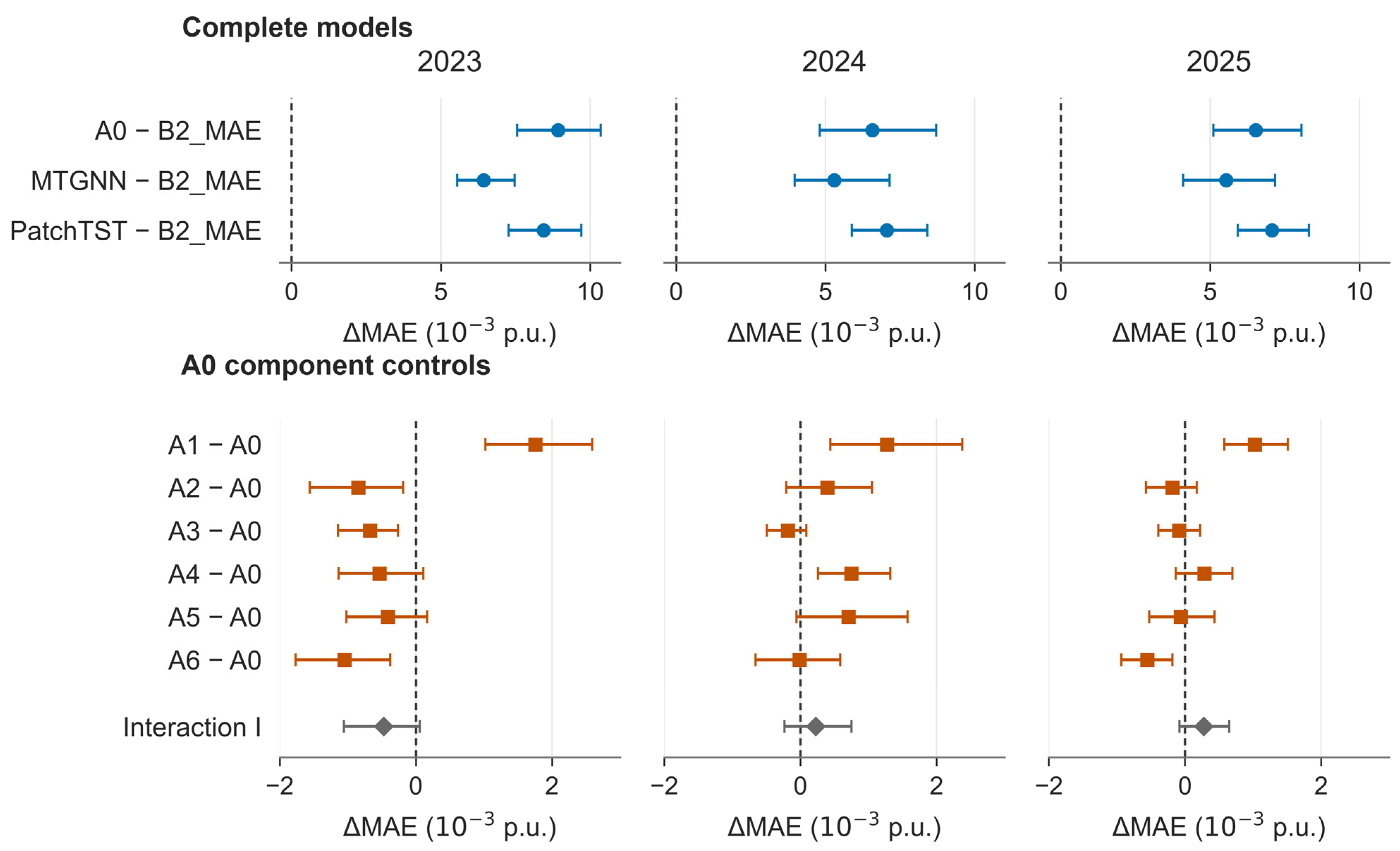
Within the simplified series, removing the recent temporal resolution (A1−A0) increases MAE by 0.001761/0.001275/0.001027 p.u. in 2023/2024/2025, and all paired intervals are above zero (Figure 5, bottom row). This supports retaining recent temporal resolution in the compact representation. B2’s lower overall error supports its use as a complete model, but does not isolate its multiscale module: B2 and A0 differ in hourly versus pooled recurrence, weather access, width, selectors, attention parameters and adapters.
Figure 5.
Paired annual MAE differences and 95% temporal intervals based on moving blocks of seven UTC target days. Top: complete-model comparisons, with positive comparator−B2_MAE differences favoring B2_MAE. Bottom: A0 component controls, with positive Aj−A0 differences favoring A0, followed by interaction I defined in Equation (3). Blue circles, orange squares and gray diamonds denote complete-model contrasts, A0 component-control contrasts and interaction I, respectively. Markers are point estimates, horizontal bars are 95% temporal intervals, and vertical dashed lines mark zero; axes use 10−3 p.u. Horizontal scales differ between rows and are shared across years within each row. B2-versus-external contrasts were calculated post hoc from the saved bootstrap draws. A-series contrasts remain conditional on A0. Complete numerical values are provided in Supplementary Data S1.
Learned constant gates (A3) have lower mean MAE than A0 in all three years; the 2023 interval excludes zero, while the other two include it. Removing donor context (A2) has mixed effects. For A5’s same-energy routing, the MAE difference changes direction across years and every interval includes zero. The context-by-gate interactions are −0.000472, +0.000228 and +0.000279 p.u.; all three intervals span zero. A6 can outperform A0 without establishing positive interaction. Within the simplified model, the value of dynamic gating, donor context and opposite-energy routing varies across comparisons. These tests do not directly ablate the corresponding B2 components. A5 still shares jointly trained parameters, so it is not evidence from independently trained wind and PV networks.
The earlier B2 gate experiment compared dynamic and learnable fixed signed gates using three paired seeds, each trained from scratch. Dynamic gates reduced mean MAE by only about 0.32% in 2024 and 0.60% in 2025, with both temporal intervals spanning zero. The intervals do not establish a consistent dynamic-gate advantage. Earlier B2 tests also found better point accuracy after removing PCGrad. Those experiments used different training procedures and task counts from the present rolling study. Their results are reported separately from the B2_MAE values in Figure 2 and Figure 5.
3.3. Joint-Low-Output Risk
The joint-low-output event occurs on 996 of 2915 daytime rows (frequency 0.341681) and 3549 of 5833 all-time rows. Daytime Brier scores are 0.055252 for Diag, 0.053299 for WithinEnergy, 0.053312 for StaticCrossGate and 0.053312 for ContextCrossGate (Table 4). WithinEnergy improves on Diag by 3.53%; ContextCrossGate improves on Diag by 3.51%. The latter comparison changes both within-energy dependence and cross-energy pairing. A post hoc comparison with WithinEnergy attributes the observed improvement to within-energy dependence; the added cross-energy benefit remains unclear.
Table 4.
Fixed-marginal joint-low-output results, averaged across models fitted with five seeds. The event occurs when both energy-group means are below 0.10 p.u. Probability bias and variogram apply to the 2915 scheduled daytime rows. Lower Brier and variogram scores are better; probability bias is better when closer to zero. The arms share identical point predictions and station marginals from the earlier B2/Diag study, separate from B2_MAE.
For daytime Brier, ContextCrossGate minus WithinEnergy is +1.25 × 10⁻⁵, with seven-day interval [−2.79 × 10⁻⁵, +5.74 × 10⁻⁵]; ContextCrossGate minus StaticCrossGate is −6.59 × 10⁻⁷, with interval [−1.60 × 10⁻⁵, +1.10 × 10⁻⁵]. Neither supports an incremental contextual cross-energy benefit. Signed probability bias worsens from +0.015783 for Diag to +0.018830 for ContextCrossGate, and the cross-energy variogram changes unfavorably from 0.016299 to 0.016304. The lower event Brier score is accompanied by poorer bias and variogram values, so calibration and dependence recovery do not improve uniformly. The accompanying data report all-time scores, sensitivity at the 0.20 threshold, reliability bins and 28-day intervals.
3.4. Reproducibility and Computational Cost
All 90 fits finished after 17–46 epochs, below the 50-epoch ceiling. Saved-checkpoint replay reproduced predictions exactly on the GPU and within 1.76 × 10⁻⁶ on the CPU, below the 10−5 tolerance. For each checkpoint, the checks used the first 128 validation and 128 test predictions. The result package contains the protocol, preprocessing, checkpoints, predictions and resampling draws needed to reproduce the annual scores and temporal intervals independently.
B2_MAE has 124,764 parameters, compared with 13,699 for A0 and A5. On an NVIDIA GeForce RTX 4090 GPU (NVIDIA Corporation, Santa Clara, CA, USA), its median training duration across nine fits covering three years and three seeds was 62.8 s (range 31.6 to 110.0 s). A0 took a median of 42.6 s (23.6 to 61.4 s). Table 5 also gives the results for MTGNN and PatchTST. Training used batches of 128, with duration varying by stopping epoch and training-set size. The timer ran from before the first epoch to the final validation-prediction export. It included validation, checkpoint saving and reloading; model construction was excluded.
Table 5.
Computational cost on an NVIDIA GeForce RTX 4090. Training time is the median [minimum, maximum] across nine fits covering all combinations of test year and seed, using training batches of 128. Forward latency is the mean for a batch-size-1, seven-station task at one 24 h lead, with inputs already on the device.
Mean forward latency was 3.8 ms for B2_MAE, 3.4 ms for A0 and 3.3 ms for A5. Each timed call used a batch of one and returned seven station outputs at a single 24 h lead. A continuous 24-step forecast was not timed. The check used training data, with 20 warm-up calls followed by five repeats of 100 synchronized calls. Inputs were prepared on the GPU before timing, excluding data preparation and transfer. Training and evaluation used Python 3.12.13, NumPy 2.4.4, PyTorch 2.12.1 + cu130 and CUDA 13.0. The timing check disabled TF32 and requested deterministic execution in warning mode; some attention and pooling kernels reported that deterministic execution was unsupported.
A0 and A5 have 89.0% fewer parameters than B2_MAE. Their forward latency is only modestly lower, and their point forecasts are less accurate. They retain matched active modules, with counted MACs of 591,760 and 592,528 per example, respectively. These estimates exclude nonlinearities, normalization and elementwise work. Parameter counts and timings on one device do not explain B2’s accuracy advantage or establish deployment costs.
4. Discussion
4.1. Scope of Architectural and Dependence Evidence
B2_MAE consistently achieves lower annual MAE than the two external baselines and the compact variants under the common protocol. The compact A1 comparison also supports retaining recent temporal resolution. These results support shared multiscale modeling. Individual B2 contributions cannot be isolated from the comparison of B2 with A0 because the models differ in hourly feature processing, width, recurrence, attention and adaptation. Historical B2 gate controls show small, uncertain dynamic-gate effects. All runs stopped before the 50-epoch ceiling. The comparison nevertheless describes performance under the shared budget and stopping rule, rather than the best achievable performance of each model family.
B2_MAE’s point-series covariance error is lower than A0’s in all twelve year-by-horizon comparisons, whereas correlation-error ordering is mixed. These metrics describe deterministic prediction trajectories and leave the diagonal conditional covariance of the marginal uncertainty head unchanged. The fixed-marginal risk study tests dependence at the output-distribution level. It improves the illustrative joint-low-output score mainly through within-energy dependence. Additional contextual cross-energy pairing and probability calibration remain unvalidated. Shared latent attention, signed message updates and output-distribution dependence therefore represent distinct mechanisms.
4.2. Proxy Data and Operational Validation Limits
The main limitation comes from generating power with ERA5 data and shared conversion assumptions. Fixed conversion parameters may produce more regular intersite relationships than a real fleet, and the targets omit curtailment, outages, heterogeneous controls and sensor errors. Matched SCADA would be needed to estimate proxy-to-measured error. Historical same-clock weather also differs from operational numerical weather prediction (NWP) in forecast errors, provider bias, revisions and availability. The nominal one-hour offset is a timing assumption for this retrospective experiment; it does not describe real-time data availability.
We assessed W-2 extraction sensitivity at the registered coordinate and four locations displaced by approximately 15 km to the north, east, south and west. Bilinear and nearest-neighbor extraction gave ten conditions, each covering the 8784 h of 2024 with the turbine conversion held fixed. Relative to the registered bilinear series, mean absolute power deviations were 0.002933 to 0.004460 p.u. for the four bilinear perturbations, 0.001719 p.u. for registered nearest-neighbor extraction and 0.006647 p.u. for the southern nearest-neighbor condition. These deviations quantify changes in simulated power caused by extraction choices. They do not identify the true plant location or estimate SCADA error. Forecast robustness after retraining was not tested, and no coordinate was selected by forecast performance.
The three complete test years cover different calendar periods. Seasonal and station results describe variation within the same seven-site simulation. Because the evaluation is retrospective and the training window expands, weather conditions and training-data volume both change between test years. Seed dispersion measures optimization variation. Transfer to new regions or operating plants therefore requires an independently specified evaluation using measured multisite power and time-stamped operational NWP.
The joint-low-output threshold is an illustrative probability diagnostic. A system shortfall also depends on demand, installed capacity, network constraints and reserve policy. Dependence errors can therefore affect shortage assessments, but storage, trading or scheduling value must be evaluated with an explicit decision model and relevant operational data [2,3,18,19,22,23]. The event scores can inform such an evaluation; decision benefits have not been quantified here.
5. Conclusions
The shared multiscale B2 architecture trained with energy-balanced MAE achieves the lowest annual mean error among ten tested implementations over 2023–2025. Its advantage over adapted MTGNN and PatchTST is consistent across the three rolling years. The compact component series supports additional recent temporal resolution, while dynamic gating, donor context and cross-energy routing show less consistent benefits. The separate fixed-marginal analysis improves joint-low-output Brier scores mainly through within-energy dependence, with no established additional cross-energy gate benefit or uniform calibration improvement. Together, the point forecasts and joint-low-output analysis characterize prediction performance on ERA5-derived power. Their relevance to plant operation requires validation with measured power and operational weather forecasts.
Supplementary Materials
The following supporting information can be downloaded at: https://www.mdpi.com/article/10.3390/electronics15204816/s1. Supplementary Data S1 contains complete numerical values for Figure 2, Figure 3, Figure 4 and Figure 5: annual scores, horizon scores, 2025 station scores and paired annual effects. Values retain the precision of the archived analysis files.
Author Contributions
Conceptualization, L.Y.; Methodology, J.Z.; Software, J.Z.; Validation, B.W. and N.F.; Formal analysis, N.F.; Resources, J.Z.; Data curation, B.W.; Writing—original draft, L.Y. and G.L.; Writing—review & editing, N.F.; Visualization, B.W.; Supervision, T.Z.; Project administration, G.L.; Funding acquisition, T.Z. All authors have read and agreed to the published version of the manuscript.
Funding
This research is supported by the project: Project No.: CHDKJ-02501148, Project Name: Intelligent Dispatching, Decision-Making and Operation for Integrated Hydro-Wind-Solar Power in the Wujiang River Basin.
Data Availability Statement
ERA5 hourly data are available from the Copernicus Climate Data Store [25]. The accompanying code and data package contains the prespecified protocol, code, derived arrays, checkpoints, predictions and numerical analyses.
Conflicts of Interest
Authors Lijun Yu, Tiancai Zuo, Jinjiang Zhou and Baochen Wang were employed by the company Guizhou Wujiang Hydropower Development Co., Ltd. The remaining authors declare that the research was conducted in the absence of any commercial or financial relationships that could be construed as a potential conflict of interest.
Abbreviations
| BiGRU | Bidirectional gated recurrent unit |
| ERA5 | Fifth-generation atmospheric reanalysis of the European Centre for Medium-Range Weather Forecasts |
| MAE | Mean absolute error |
| MHA | Multi-head attention |
| NWP | Numerical weather prediction |
| PV | Photovoltaic |
| RMSE | Root-mean-square error |
| SCADA | Supervisory control and data acquisition |
References
- ElRobrini, F.; Bukhari, S.M.S.; Zafar, M.H.; Al-Tawalbeh, N.; Akhtar, N.; Sanfilippo, F. Federated Learning and Non-Federated Learning Based Power Forecasting of Photovoltaic/Wind Power Energy Systems: A Systematic Review. Energy AI 2024, 18, 100438. [Google Scholar] [CrossRef] [Scilit]
- Olauson, J.; Viotti, O.; Huss, J. The HEFTCom2024 Winning Model: A Stacked CatBoost Approach for Probabilistic Wind and Solar Power Forecasting. Int. J. Forecast. 2026, 42, 724–735. [Google Scholar] [CrossRef] [Scilit]
- Browell, J.; van der Meer, D.; Kälvegren, H.; Haglund, S.; Simioni, E.; Bessa, R.J.; Wang, Y. The Hybrid Renewable Energy Forecasting and Trading Competition 2024. Int. J. Forecast. 2026, 42, 709–723. [Google Scholar] [CrossRef] [Scilit]
- Bashir, T.; Wang, H.; Tahir, M.; Zhang, Y. Wind and Solar Power Forecasting Based on Hybrid CNN-ABiLSTM, CNN-Transformer-MLP Models. Renew. Energy 2025, 239, 122055. [Google Scholar] [CrossRef] [Scilit]
- Gao, Y.; Liang, L.; Su, T.; Pan, M. An Embedded Spatiotemporal Hybrid Model Integrating Multi-Graphs and Attention-Driven Fusion for Single- and Multi-Site Photovoltaic Power Forecasting. Energy Convers. Manag. 2025, 336, 119897. [Google Scholar] [CrossRef] [Scilit]
- Hasnat, M.A.; Asadi, S.; Alemazkoor, N. A Graph Attention Network Framework for Generalized-Horizon Multi-Plant Solar Power Generation Forecasting Using Heterogeneous Data. Renew. Energy 2025, 243, 122520. [Google Scholar] [CrossRef] [Scilit]
- Li, Z.; Ye, L.; Song, X.; Luo, Y.; Pei, M.; Wang, K.; Yu, Y.; Tang, Y. Heterogeneous Spatiotemporal Graph Convolution Network for Multi-Modal Wind-PV Power Collaborative Prediction. IEEE Trans. Power Syst. 2024, 39, 5591–5608. [Google Scholar] [CrossRef] [Scilit]
- Jiang, J.; He, Y.; Zhang, Y.; Yan, J.; Lv, Z.; Liu, Z.; Dai, H.; Zhen, Z. A Multi-Task Learning and GCN-Transformer-Based Forecasting Method for Day-Ahead Power of Wind-Solar Clusters. Electronics 2026, 15, 462. [Google Scholar] [CrossRef] [Scilit]
- Vázquez Pombo, D.; Rincón, M.J.; Bacher, P.; Bindner, H.W.; Spataru, S.V.; Sørensen, P.E. Assessing Stacked Physics-Informed Machine Learning Models for Co-Located Wind-Solar Power Forecasting. Sustain. Energy Grids Netw. 2022, 32, 100943. [Google Scholar] [CrossRef] [Scilit]
- Camal, S.; Teng, F.; Michiorri, A.; Kariniotakis, G.; Badesa, L. Scenario Generation of Aggregated Wind, Photovoltaics and Small Hydro Production for Power Systems Applications. Appl. Energy 2019, 242, 1396–1406. [Google Scholar] [CrossRef] [Scilit]
- Lindberg, O.; Lingfors, D.; Arnqvist, J.; van der Meer, D.; Munkhammar, J. Day-Ahead Probabilistic Forecasting at a Co-Located Wind and Solar Power Park in Sweden: Trading and Forecast Verification. Adv. Appl. Energy 2023, 9, 100120. [Google Scholar] [CrossRef] [Scilit]
- Couto, A.; Estanqueiro, A. Wind Power Plants Hybridised with Solar Power: A Generation Forecast Perspective. J. Clean. Prod. 2023, 423, 138793. [Google Scholar] [CrossRef] [Scilit]
- Caruana, R. Multitask Learning. Mach. Learn. 1997, 28, 41–75. [Google Scholar] [CrossRef] [Scilit]
- Chen, Y.; Xiao, J.-W.; Wang, Y.-W.; Li, Y. Regional Wind-Photovoltaic Combined Power Generation Forecasting Based on a Novel Multi-Task Learning Framework and TPA-LSTM. Energy Convers. Manag. 2023, 297, 117715. [Google Scholar] [CrossRef] [Scilit]
- Puzhuang, L.; Mohamed Kamari, N.A.B.; Mohd Zaman, M.H.; Zulkifley, M.A. A Novel Multi-Task Learning Framework TBM with Shared and Task-Specific Features Fusion in Regional Wind-Solar-Load Joint Forecasting. Energy Convers. Manag. X 2025, 28, 101346. [Google Scholar] [CrossRef] [Scilit]
- Abid, M.S.; Ahshan, R.; Al-Abri, M.; Al Abri, R. Spatiotemporal Forecasting of Solar and Wind Energy Production: A Robust Deep Learning Model with Attention Framework. Energy Convers. Manag. X 2025, 26, 100919. [Google Scholar] [CrossRef] [Scilit]
- Özüpak, Y.; Alpsalaz, F.; Aslan, E.; Uzel, H. An Interpretable Multi-Level Stacking Framework for Photovoltaic Power Prediction and Fault Analysis. Energy 2026, 360, 141715. [Google Scholar] [CrossRef] [Scilit]
- Zhong, J.; Zhao, J.; Fei, Z.; Li, Z.; Pouresmaeil, E.; Su, Y.; Xie, L.; Cao, Y. Huber-CVaR-Based Distributionally Robust Bilevel Optimization for Energy Hubs Integrating Heterogeneous Flexibility Resources. Appl. Energy 2026, 426, 128587. [Google Scholar] [CrossRef] [Scilit]
- Yu, J.; Zhao, J.; Zhong, J.; Lin, Z.; Xu, Y.; Peng, Y.; Cai, Y.; Cao, L.; Zhang, M.; Cao, Y. Towards Fairness and Low-Carbon Operation of Energy Hub: A Multi-Objective Optimization Framework with Energy–Carbon Bidirectional Coupling and Heterogeneous Uncertainties. Appl. Energy 2026, 409, 127475. [Google Scholar] [CrossRef] [Scilit]
- Chen, Z.; Badrinarayanan, V.; Lee, C.-Y.; Rabinovich, A. GradNorm: Gradient Normalization for Adaptive Loss Balancing in Deep Multitask Networks. Proc. Mach. Learn. Res. 2018, 80, 794–803. [Google Scholar]
- Yu, T.; Kumar, S.; Gupta, A.; Levine, S.; Hausman, K.; Finn, C. Gradient Surgery for Multi-Task Learning. Adv. Neural Inf. Process. Syst. 2020, 33, 5824–5836. [Google Scholar]
- Soon, K.L.; Soon, L.T.; Pang, W.L.; Goh, H.H.; Sooriamoorthy, D. Conformalized Uncertainty Quantification for Joint Solar-Wind Power Forecasting in Reliable Grid Integration. J. Comput. Sci. 2026, 98, 102902. [Google Scholar] [CrossRef] [Scilit]
- Scheuerer, M.; Hamill, T.M. Variogram-Based Proper Scoring Rules for Probabilistic Forecasts of Multivariate Quantities. Mon. Weather Rev. 2015, 143, 1321–1334. [Google Scholar] [CrossRef] [Scilit]
- Hersbach, H.; Bell, B.; Berrisford, P.; Hirahara, S.; Horányi, A.; Muñoz-Sabater, J.; Nicolas, J.; Peubey, C.; Radu, R.; Schepers, D.; et al. The ERA5 Global Reanalysis. Q. J. R. Meteorol. Soc. 2020, 146, 1999–2049. [Google Scholar] [CrossRef] [Scilit]
- Copernicus Climate Change Service. ERA5 Hourly Data on Single Levels from 1940 to Present; Copernicus Climate Data Store: Reading, UK, 2018. [Google Scholar] [CrossRef]
- Cho, K.; van Merriënboer, B.; Gulcehre, C.; Bahdanau, D.; Bougares, F.; Schwenk, H.; Bengio, Y. Learning Phrase Representations Using RNN Encoder–Decoder for Statistical Machine Translation. In Proceedings of the 2014 Conference on Empirical Methods in Natural Language Processing (EMNLP), Doha, Qatar, 25–29 October 2014; pp. 1724–1734. [Google Scholar] [CrossRef] [Scilit]
- Wu, Z.; Pan, S.; Long, G.; Jiang, J.; Chang, X.; Zhang, C. Connecting the Dots: Multivariate Time Series Forecasting with Graph Neural Networks. In Proceedings of the 26th ACM SIGKDD International Conference on Knowledge Discovery & Data Mining, Virtual, 23–27 August 2020; pp. 753–763. [Google Scholar] [CrossRef] [Scilit]
- Nie, Y.; Nguyen, N.H.; Sinthong, P.; Kalagnanam, J. A Time Series Is Worth 64 Words: Long-Term Forecasting with Transformers. In Proceedings of the International Conference on Learning Representations (ICLR), Kigali, Rwanda, 1–5 May 2023; Available online: https://arxiv.org/abs/2211.14730 (accessed on 11 September 2026).
- Hyndman, R.J.; Koehler, A.B. Another Look at Measures of Forecast Accuracy. Int. J. Forecast. 2006, 22, 679–688. [Google Scholar] [CrossRef] [Scilit]

Disclaimer/Publisher’s Note: The statements, opinions and data contained in all publications are solely those of the individual author(s) and contributor(s) and not of MDPI and/or the editor(s). MDPI and/or the editor(s) disclaim responsibility for any injury to people or property resulting from any ideas, methods, instructions or products referred to in the content. |
© 2026 by the authors. Licensee MDPI, Basel, Switzerland. This article is an open access article distributed under the terms and conditions of the Creative Commons Attribution (CC BY) license.