Online Inertia Estimation for Supply-Side Nodes Using ARX-IG-UKF

Abstract

Conventional unscented Kalman filter (UKF)-based inertia estimators are constrained by slow convergence within the limited inertial response window and a fixed measurement noise variance that cannot capture time-varying uncertainty during disturbances. This paper proposes ARX-IG-UKF, an online nodal inertia estimation method combining autoregressive modeling with exogenous inputs (ARX) for initialization and inverse-gamma (IG) noise adaptation. First, an ARX model fitted to early post-disturbance power frequency data provides an initial nodal inertia estimate. This estimate initializes a state-space model describing the inertial responses of synchronous generators and renewable generation units, reducing the convergence time required for short-window estimation. An IG distribution is then used to update the measurement noise covariance online in response to deviations associated with primary frequency regulation. The adaptive covariance is incorporated into the UKF to reduce the influence of non-inertial dynamics and recursively estimate nodal inertia. Simulation studies demonstrate consistent convergence and stable estimates under a range of operating conditions, supporting the applicability of the method to online nodal inertia identification in complex operating scenarios.

1. Introduction

As the penetration of renewable generation increases, conventional synchronous generators are increasingly displaced by power-electronic-interfaced resources. Variations in renewable power output and changes in unit commitment have led to a gradual decline in power system inertia [1,2,3,4]. Under low-inertia conditions, the system is less able to withstand active power disturbances, causing the frequency nadir to approach or even exceed its security threshold. Fast and accurate inertia estimation is therefore essential for system operators to implement frequency-support and emergency control measures effectively [5,6,7].

Power system inertia estimation methods can be broadly divided into two categories: methods based on ambient measurements and those based on disturbance event measurements [8]. Inertia estimation using ambient data, however, remains challenging. To the best of our knowledge, Ref. [9] was the first to identify system inertia from ambient measurements and developed a statistical model to characterize the relationship between system inertia and steady-state frequency variations. Ref. [10] proposed a closed-loop identification method that estimates the power system inertia constant by applying a known probing signal. Ref. [11] derived a combined model of inertial response and primary frequency regulation. A high-order model was then used to fit the transfer functions between multiple inputs and outputs, and the inertia time constant was obtained from the system response to a step input.

Compared with ambient-data-based approaches, disturbance-event-based inertia estimation has a broader range of applications and a more mature engineering foundation. Ref. [12] used synchronized post-disturbance measurements and dynamic mode decomposition (DMD) to extract system dynamics and estimate inertia in multi-area power systems. Its computational efficiency, however, limits its use for rapid online estimation. To address this issue, Ref. [13] introduced streaming dynamic mode decomposition (sDMD), which reduces computational and storage costs while maintaining estimation accuracy, thereby enabling efficient real-time inertia identification.

Recent advances in phasor measurement units (PMUs) have made online estimation of power system inertia feasible. PMUs provide the phase angles of bus voltages and currents, from which real-time frequency can be calculated and used as a state variable. This capability has supported the development of various state-estimation methods for online inertia estimation, most of which are based on the Kalman filter (KF) [14,15,16]. As a linear estimator, however, the KF cannot handle the nonlinear relationship between the inertia parameter, when treated as an unknown state, and system frequency dynamics. Ref. [17], therefore, introduced the extended Kalman filter (EKF), which locally linearizes the nonlinear model to jointly estimate generator dynamic states and parameters such as inertia online. Using nodal frequency measurements, Ref. [18] constructed a corresponding state-space model and estimated inertia within an unscented Kalman filter (UKF) framework. Unlike the EKF, which relies on local model linearization, the UKF propagates a set of sigma points to preserve higher-order information about the state distribution, allowing faster and more accurate inertia tracking during nonlinear estimation. This method, however, does not account for the effect of current limiting on inertial support. Ref. [6] addressed this limitation by incorporating a current limiter into the inertia identification model and introducing an adaptive unscented Kalman filter (AUKF), thereby improving tracking accuracy and robustness. Nevertheless, these methods remain sensitive to the choice of estimation window length. A long window allows primary frequency regulation to exert a greater influence on the measured response, reducing inertia estimation accuracy; a short window, by contrast, provides insufficient time for the filter to converge. Moreover, when the specified initial inertia differs substantially from its true value, the limited convergence rate of the UKF may prevent the estimate from approaching the true value within the finite inertial response window.

To address the remaining limitations of existing methods, this paper proposes a power system inertia estimation method termed ARX-IG-UKF. The main contributions are as follows:

• The frequency-response equations of renewable generation nodes and conventional synchronous-generator nodes are combined to formulate a unified state-space model linking inertia constants with frequency dynamics. This model describes the relationship between frequency response and inertial support in renewable-rich power systems.
• To reduce the sensitivity of Kalman-filter-based inertia identification to the specified initial inertia, an autoregressive model with exogenous inputs (ARX) is used to obtain a preliminary estimate of nodal inertia. This estimate provides a more appropriate initial condition for subsequent recursive state estimation.
• A conventional UKF uses a fixed measurement noise variance and therefore assumes constant confidence in frequency measurements. This assumption limits its ability to suppress the influence of non-inertial dynamics, such as primary frequency regulation during the later stage of a disturbance. An adaptive measurement noise variance estimation method based on an inverse-gamma (IG) prior is therefore introduced and incorporated into the UKF, reducing the effect of non-inertial dynamics on inertia identification.

2. Inertial Response and State-Space Modeling

As the penetration of renewable generation increases, the inherent inertia of the power system continues to decline. Consequently, disturbances produce a higher rate of change of frequency (RoCoF), a lower-frequency nadir, and a reduced frequency stability margin [2,19,20]. System inertia is also distributed unevenly because the generation mix and operating conditions vary across regions, resulting in pronounced spatial differences. A system-wide equivalent inertia alone, therefore, cannot adequately characterize the ability of individual nodes to withstand power disturbances. Accurate estimation of nodal or regional inertia is essential for frequency security assessment, stability analysis, and control resource allocation in low-inertia power systems [8,21].

2.1. Inertial Response at Generation Nodes

The inertia of a synchronous generator is provided mainly by the mechanical kinetic energy stored in its rotor and other components rotating on the same shaft. The inertia constant reflects the capacity of this stored energy to resist active power imbalances [22]. When an active power disturbance disrupts the balance between generation and demand, the rotor releases stored kinetic energy or absorbs surplus electrical energy from the grid, thereby contributing to the restoration of system power balance.

Unlike conventional synchronous generators, which naturally participate in frequency response through the kinetic energy stored in their rotors, renewable generation units are typically connected to the grid through power electronic converters. The lack of direct electromechanical coupling between their internal energy reserves and system frequency prevents these units from inherently producing an inertial response similar to that of synchronous generators [23]. Their inertia contribution, therefore, depends mainly on the ability of the converter control to regulate the available energy. Under virtual inertia control, the controller adjusts active power output according to the rate of change of frequency, thereby emulating the inertial response of a synchronous generator. For unified modeling, this control-based inertia can be represented by an equivalent inertia constant [23,24] and described using the swing equation:

$$2H_i{\displaystyle \frac{d}{\mathit{dt}}}({\displaystyle \frac{\Delta f_i}{f_0}})=P_m-P_e-D{\displaystyle \frac{\Delta f_i}{f_0}}$$

(1)

where f₀ is the rated system frequency; H_i is the equivalent inertia time constant of the node connected to a synchronous generator; Δf is the nodal frequency deviation; d(Δf/f₀)/dt is the per-unit rate of change of nodal frequency; P_m is the per-unit mechanical power; P_e is the per-unit electrical power; and D is the per-unit damping coefficient.

During the initial stage following a disturbance, the governor has not yet responded [25,26], allowing the mechanical power P_m to be treated as constant. Moreover, because the damping coefficient D is small and Δf ≈ 0, the swing equation can be simplified as follows:

$$2H_i{\displaystyle \frac{d}{\mathit{dt}}}({\displaystyle \frac{\Delta f_i}{f_0}})=P_{\mathit{set}}-P_e$$

(2)

where P_set is the pre-disturbance per-unit steady-state power and is treated as a constant, whereas the electrical power P_e varies with time.

2.2. State-Space Modeling of Nodal Inertia

To recursively estimate nodal inertia, a state-space model describing the frequency power coupling at each node is derived from the swing equation. The unknown equivalent inertia constant H of the target node and the frequency deviation Δf form the state vector x_k; the post-disturbance active power deviation ΔP is taken as the input u_k; the frequency deviation measured by the PMU is used as the measurement z_k. These variables are defined as follows:

$$x_k=\left[\begin{array}{c}{H}_k\\ \Delta f_k\end{array}\right],\hspace{1em}{u}_k=\Delta P_k,\hspace{1em}{z}_k=\Delta f_k$$

(3)

The system input u_k is given by

$$u_k=\Delta P_k=P_{\mathit{set}}-\mathrm{Re}[{\displaystyle \frac{3}{2}}(V_k{e}^{j{\theta }_{V_k}})(\overline{I_k{e}^{j{\theta }_{I_k}}})]/S_n$$

(4)

where S_n is the rated capacity of the generation unit; $V_k{e}^{j{\theta }_{V_k}}$ denotes the bus phase-voltage phasor; and $\overline{I_k{e}^{j{\theta }_{I_k}}}$ denotes the complex conjugate of the bus-current phasor. The swing equation then gives the continuous-time frequency dynamics model:

$${\displaystyle \frac{d\Delta f}{\mathit{dt}}}={\displaystyle \frac{f_0}{2H}}\{P_{\mathit{set}}-\mathrm{Re}[{\displaystyle \frac{3}{2}}(V_k{e}^{j{\theta }_{V_k}})(\overline{I_k{e}^{j{\theta }_{I_k}}})]/S_n\}$$

(5)

Applying first-order Euler discretization to the continuous-time model yields the following state-transition equation:

$$\left\{\begin{array}{c}{H}_{k+1}=H_k\\ \Delta f_{k+1}=\Delta f_k+{\displaystyle \frac{f_0}{2H_k}}{u}_k\Delta t\end{array}\right.$$

(6)

where Δt is the sampling interval.

3. ARX-IG-UKF-Based Method for Nodal Inertia Estimation

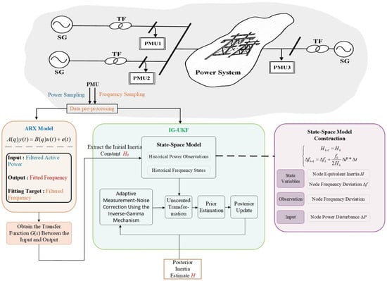
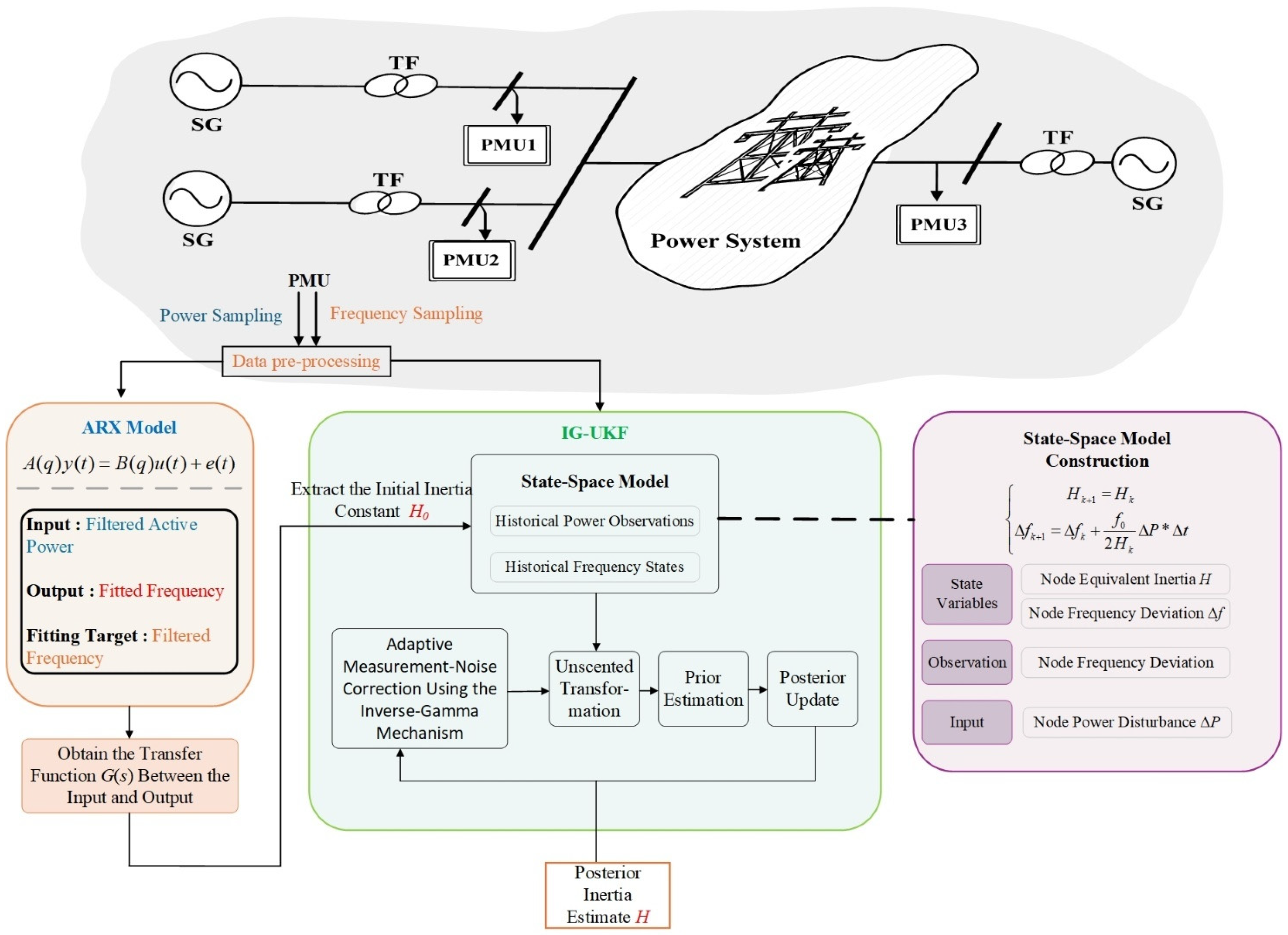
The ARX-IG-UKF framework is illustrated in Figure 1. It comprises two stages: inertia initialization and adaptive recursive estimation. During the initialization stage, an ARX model is fitted to the power and frequency data recorded immediately after a disturbance to obtain a preliminary estimate of nodal inertia. This estimate is then used to initialize the subsequent state-space model. During the recursive estimation stage, the state equation linking the nodal inertia constant to frequency dynamics is formulated according to the mechanisms described above. The power disturbance is treated as the input, while the frequency deviation serves as both a state variable and a measurement. Nodal inertia is then estimated recursively within the UKF framework. To mitigate the effect of an assumed fixed noise covariance on the filtering results, an inverse-gamma prior is assigned to the frequency measurement noise variance, which is updated recursively from the measurement residuals. Combining this adaptive noise estimation with the UKF enables the ARX-IG-UKF method to estimate nodal inertia accurately.

Figure 1. ARX-IG-UKF-based inertia estimation framework.

3.1. ARX-Based Initial Estimation of Nodal Inertia

Before IG-UKF-based inertia estimation, an ARX model is introduced to obtain an initial inertia estimate. Inertial response occurs mainly during the early stage of a disturbance. Primary frequency regulation, reactive power control, and other dynamic modes subsequently begin to affect the frequency response, meaning that the information most relevant to inertia identification is concentrated in the initial power frequency dynamics. If the IG-UKF is applied directly with an initial inertia value that differs substantially from the true value, the filter may not converge within the limited inertial response window, reducing the accuracy of subsequent estimates. The proposed method, therefore, applies short-window ARX identification to the early power frequency response and uses the resulting inertia estimate to initialize the IG-UKF. This strategy provides a better-informed initial condition for nonlinear recursive estimation, reducing the filter’s sensitivity to initialization and improving identification stability under dynamic disturbances.

Conventional model-order selection criteria, such as the Akaike information criterion (AIC), primarily assess model fit. In the proposed algorithm, however, the ARX model is intended to provide a timely initial inertia estimate rather than maximize estimation accuracy. Although a higher model order may improve the fit to the frequency response, it also increases the number of parameters to be estimated and the computational cost. A first-order ARX model is therefore used for initialization, reducing computational effort and providing the initial estimate quickly while retaining adequate accuracy.

The general form of the ARX model is

$$\left\{\begin{array}{c}A(q^{-1})y(t)=B(q^{-1})u(t-n_k)+e(t)\\ A\left(q\right)=1+a_1{q}^{-1}+\dots +a_{n_a}{q}^{-n_a}\\ B\left(q\right)=b_1+b_2{q}^{-1}+\dots +b_{n_b}{q}^{-n_b+1}\end{array}\right.$$

(7)

where q⁻¹ is the unit-delay operator; y(t) is the system output; u(t) is the external input; e(t) is the model residual; a_i is the autoregressive coefficient describing the dependence of the frequency response on its past values; b_i is the exogenous-input coefficient characterizing the effect of active power deviations on frequency dynamics; n_a and n_b are the orders of the output and input terms, respectively; and n_k is the input delay.

The ARX model is constructed with the power deviation as the input and the frequency deviation as the output to be fitted. To estimate its parameters, the model is rewritten in linear regression form:

y(t) = φ^T(t)θ + e(t)

(8)

where the regression vector φ(k) and the unknown parameter vector θ are expanded as

$$\left\{\begin{array}{c}\phi (t)=[-y(t-1)\cdots -y(t-n_a )u(t-n_k)\\ \cdots u(t-n_k-n_b+1){]}^T\\ \theta ={[a_1\cdots a_{n_a} b_1\cdots b_{n_b}]}^T\end{array}\right.$$

(9)

For an identification window of length N, the regression matrix is assembled as follows:

Y = Φθ + E

(10)

where

$$Y=\left[\begin{array}{c}y(k_0)\\ y(k_0+1)\\ ⋮\\ y(N)\end{array}\right],\hspace{1em}\mathsf{\Phi }=\left[\begin{array}{c}{\phi }^T(k_0)\\ {\phi }^T(k_0+1)\\ ⋮\\ {\phi }^T(N)\end{array}\right]$$

(11)

The least-squares solution in matrix form is

$$\widehat{\theta }={({\mathsf{\Phi }}^T\mathsf{\Phi })}^{-1}{\mathsf{\Phi }}^{T}Y$$

(12)

Once the ARX parameters have been identified, the discrete transfer function between the model input and output is obtained as

$$G_d(q^{-1})={\displaystyle \frac{Y(q^{-1})}{U(q^{-1})}}=q^{-n_k}{\displaystyle \frac{B(q^{-1})}{A(q^{-1})}}$$

(13)

For the first-order ARX model, this becomes

$$G_d(q^{-1})={\displaystyle \frac{b_1}{1+a_1{q}^{-1}}}$$

(14)

G_d(q⁻¹) denotes the transfer function between the model input and output. It describes the dynamic relationship between active power deviation and frequency response, providing a basis for extracting inertia-related characteristics. To relate the ARX identification result to the continuous-time swing equation, the discrete transfer function is mapped to the continuous s-domain through a bilinear transformation, yielding

$$G(s)={\displaystyle \frac{b_1^{\prime }s+b_2^{\prime }}{s+a_1^{\prime }}}$$

(15)

Applying a step input of amplitude ΔP_step to the transfer function G(s) and taking the inverse Laplace transform yields the frequency response f_step(t):

$$f_{\mathrm{step}}(t)={\mathcal{L}}^{-1}\left[G_c(s){\displaystyle \frac{\Delta P_{\mathrm{step}}}{s}}\right]$$

(16)

The initial inertia estimate H₀ is then obtained as

$$H_0={\displaystyle \frac{f_0{P}_{\mathrm{step}}}{2(d{f}_{\mathrm{step}}(t)/\mathit{dt})}}$$

(17)

The accuracy of the initial inertia estimate is sensitive to the identification window length. A sensitivity study was therefore conducted using 36 randomly selected generator cases from the 9-bus and 68-bus systems, with inertia constants ranging from 1 to 20 s. Data segments of different lengths were supplied to the ARX model to examine the effect of window length on the initial estimate. The results are summarized in Table 1. Negative inertia estimates produced by the ARX model were classified as identification failures.

Table 1. Relative errors and identification failures for different ARX window lengths.

Window Length (s)	MAPE (%)	Number of Failures
0.5	36.77	4
1	10.85	0
1.5	15.19	0
2	18.86	0
2.5	22.00	0
3	25.20	0
3.5	27.95	0
4	30.31	0

3.2. IG-Based Adaptive UKF Algorithm

The ARX model provides an initial estimate of nodal inertia from the frequency response, but its identification accuracy is sensitive to the window length. To reduce the errors caused by an arbitrary choice of the identification window, the IG-UKF is initialized with the ARX estimate and then used to recursively estimate the nodal inertia constant and frequency state.

As the estimation window advances, primary frequency regulation increasingly contributes to the system frequency response, causing the actual response to deviate from the inertial response model. A conventional UKF uses a fixed measurement noise covariance and therefore assigns constant confidence to the measured frequency throughout the identification process. Consequently, frequency measurements affected by primary frequency regulation continue to update the inertia state, introducing bias into the resulting estimate.

In contrast, the IG-based noise model represents the measurement noise variance probabilistically and updates it online using the residual between the estimated and measured frequencies. As the influence of primary frequency regulation becomes more pronounced, the estimated measurement noise variance increases, causing the UKF to assign less weight to the frequency measurements. This adaptive adjustment reduces the interference of non-inertial response modes with inertia identification.

Based on the state-space model described in Section 2, process noise and measurement noise are introduced into the state and measurement equations to account for prediction errors caused by unmodeled dynamics and frequency measurement errors from the PMU, respectively:

$$\left\{\begin{array}{c}{x}_{k+1}=f(x_k,u_k)+w_k\\ z_k=h(x_k)+{\epsilon }_k\end{array}\right.$$

(18)

where

$$\left\{\begin{array}{c}f(x_k,u_k)=\left[\begin{array}{c}{H}_k\\ \Delta f_k+{\displaystyle \frac{f_0}{2H_k}}\{P_{\mathit{set}}-{\displaystyle \frac{\mathrm{Re}[\frac{3}{2}(V_k{e}^{j{\theta }_{V_k}})(\overline{I_k{e}^{j{\theta }_{I_k}}})]}{S_n}}\}\Delta t\end{array}\right]\\ h(x_k)=\Delta f_k\end{array}\right.$$

(19)

The terms w_k and ε_k denote the process noise and measurement noise, respectively.

The IG-UKF approximates the state distribution by constructing sigma points and propagating them directly through the nonlinear state and measurement functions, thereby improving the approximation of the transformed state statistics. Given the posterior state estimate ${\widehat{x}}_{k-1}$ at the previous time step as the mean and its covariance P_k−1 for an n-dimensional state, a set of 2n + 1 sigma points is generated as follows:

$$\left\{\begin{array}{c}{\chi }_{k-1}^0={\widehat{x}}_{k-1}\\ {\chi }_{k-1}^i={\widehat{x}}_{k-1}+{\left[\sqrt{(n+\lambda )P_{k-1}}\right]}_i,\hspace{1em}i=1,\cdots ,n\\ {\chi }_{k-1}^{i+n}={\widehat{x}}_{k-1}-{\left[\sqrt{(n+\lambda )P_{k-1}}\right]}_i,\hspace{1em}i=1,\cdots ,n\end{array}\right.$$

(20)

where λ is the scaling parameter, ${\left[\sqrt{(n+\lambda )P_{k-1}}\right]}_i$ denotes the i th column of the matrix square root, and n is the state dimension.

Given the current input u_k, the sigma points at time step k − 1 are propagated through the nonlinear state function to obtain the predicted sigma points at time step k:

$${\chi }_{k|k-1}^i=f({\chi }_{k-1}^i,u_k),\hspace{1em}i=0,\cdots ,2n$$

(21)

The a priori state estimate at time step k is obtained as the weighted mean of the transformed sigma points. The corresponding a priori state covariance matrix is computed from their deviations from the predicted state mean:

$$\left\{\begin{array}{c}{\widehat{x}}_{k|k-1}={\displaystyle {\displaystyle \sum }_{i=0}^{2n}}{W}_i^m{\chi }_{k|k-1}^i\\ P_{k|k-1}={\displaystyle {\displaystyle \sum }_{i=0}^{2n}}{W}_i^c({\chi }_{k|k-1}^i-{\widehat{x}}_{k|k-1}){({\chi }_{k|k-1}^i-{\widehat{x}}_{k|k-1})}^T+Q\end{array}\right.$$

(22)

where $W_i^m$ and $W_i^c$ are the mean and covariance weights, respectively, associated with the i th sigma point; and Q is the process noise covariance matrix, which accounts for uncertainty in the state prediction. The formulas for the weights $W_i^m$ and $W_i^c$ are given in [27].

The measurement noise variance R_k represents the uncertainty of the measured frequency relative to the inertial response model. As primary frequency regulation progressively contributes to the response during nodal inertia estimation, the measurement noise variance R_k becomes time-varying. It is therefore treated as a random variable to be estimated recursively online, within a correspondingly adapted and simplified Bayesian framework. The joint posterior distribution of the current state and measurement-noise variance satisfies

p(x_k,R_k|Z_1:k) ∝ p(z_k|x_k,R_k)p(x_k|Z_1:k−1)p(R_k|Z_1:k−1)

(23)

where p(x_k|Z_1:k−1) is the prior state distribution obtained directly from the UKF prediction, p(R_k|Z_1:k−1) is the prior distribution of the measurement noise variance, and p(z_k|x_k,R_k) is the frequency-measurement likelihood.

Joint inference of the posterior distributions of the state and measurement noise variance would substantially increase computational complexity and the resources required for online estimation. A sequential approximate solution is therefore adopted: the UKF performs nonlinear recursive state estimation, while the measurement noise variance is updated separately using the IG prior. The resulting variance estimate is then fed back into the UKF measurement update.

Assuming Gaussian measurement noise and using the measurement function h(x), the frequency-measurement likelihood p(z_k|x_k,R_k) can be expressed as

$$p(z_k|x_k,R_k)={\displaystyle \frac{1}{\sqrt{2\pi R_k}}}\exp \left[-{\displaystyle \frac{{(z_k-h(x_k))}^2}{2R_k}}\right]$$

(24)

To predict the unknown measurement noise variance in real time, an inverse-gamma distribution is assigned as the conjugate prior for R_k:

R_k∼IG(α_k,β_k)

(25)

where α_k and β_k are the shape and scale parameters of the inverse-gamma distribution, respectively. The hyperparameters ν_k and τ_k are further introduced as

$${\alpha }_k={\displaystyle \frac{{\nu }_k}{2}}+1,\hspace{1em}{\beta }_k={\displaystyle \frac{{\tau }_k}{2}}$$

(26)

The probability density function is then expressed as

$$p(R_k|{\nu }_k,{\tau }_k)={\displaystyle \frac{{(\frac{{\tau }_k}{2})}^{\frac{{\nu }_k}{2}+1}}{\mathsf{\Gamma }(\frac{{\nu }_k}{2}+1)}}{R}_k^{-({\displaystyle \frac{{\nu }_k}{2}}+2)}\exp (-{\displaystyle \frac{{\tau }_k}{2R_k}}),\hspace{1em}{R}_k>0$$

(27)

To make the measurement noise estimate more responsive to changes in the current measurements, a forgetting factor ρ is introduced when propagating the IG posterior parameters from the previous time step to the prior parameters at the current time step:

$$\left\{\begin{array}{c}{\nu }_k^{-}=\rho {\nu }_{k-1}^{+}\\ {\tau }_k^{-}=\rho {\tau }_{k-1}^{+}\end{array}\right.$$

(28)

where ρ ∈ (0,1] is the forgetting factor controlling how much historical noise information is retained in the current estimate. The parameters ${\nu }_{k-1}^{+}$ and ${\tau }_{k-1}^{+}$ are the posterior parameters at time step k − 1, whereas ${\nu }_k^{-}$ and ${\tau }_k^{-}$ are the corresponding prior parameters at time step k. The measurement noise variance used in the UKF measurement update is obtained from the IG posterior parameters at the previous time step as

$${\widehat{R}}_k^{-}=E[R_k|Z_{1:k-1}]={\displaystyle \frac{{\tau }_{k-1}^{+}}{{\nu }_{k-1}^{+}}}$$

(29)

${\widehat{R}}_k^{-}$ denotes the measurement noise variance at the current time step, predicted from the posterior parameters at the previous time step.

After the a priori state estimate has been obtained, the transformed sigma points are propagated through the measurement function to obtain the predicted measurement sigma points γ_k|k−1, establishing the statistical relationship between the predicted state and the actual measurement:

$${\gamma }_{k|k-1}^i=h({\chi }_{k|k-1}^i),\hspace{1em}i=0,\cdots ,2n$$

(30)

Weighted summation similarly yields the predicted measurement mean ${\widehat{z}}_{k|k-1}$, the measurement covariance P_zz,k, and the cross-covariance P_xz,k between the state-prediction and measurement-prediction errors:

$$\left\{\begin{array}{c}{\widehat{z}}_{k|k-1}={\displaystyle {\displaystyle \sum }_{i=0}^{2n}}{W}_i^m{\gamma }_{k|k-1}^i\\ P_{\mathit{zz},k}={\displaystyle {\displaystyle \sum }_{i=0}^{2n}}{W}_i^c\left({\gamma }_{k|k-1}^i-{\widehat{z}}_{k|k-1}\right){\left({\gamma }_{k|k-1}^i-{\widehat{z}}_{k|k-1}\right)}^T+{\widehat{R}}_k^{-}\\ P_{\mathit{xz},k}={\displaystyle {\displaystyle \sum }_{i=0}^{2n}}{W}_i^c({\chi }_{k|k-1}^i-{\widehat{x}}_{k|k-1}){({\gamma }_{k|k-1}^i-{\widehat{z}}_{k|k-1})}^T\end{array}\right.$$

(31)

The measurement noise variance obtained from the IG recursion enters the measurement-covariance calculation directly. An increase in ${\widehat{R}}_k^{-}$ raises the measurement covariance and reduces the subsequent Kalman gain, thereby weakening the correction applied to the state estimate by the frequency measurement.

The Kalman gain K_k is calculated as

$$K_k=P_{\mathit{xz},k}{P}_{\mathit{zz},k}^{-1}$$

(32)

The state is then corrected using the measured frequency and the Kalman gain:

$$\left\{\begin{array}{c}{\widehat{x}}_k={\widehat{x}}_{k|k-1}+K_k\left(z_k-{\widehat{z}}_{k|k-1}\right)\\ P_k=P_{k|k-1}-K_k{P}_{\mathit{zz},k}{K}_k^T\end{array}\right.$$

(33)

where $z_k-{\widehat{z}}_{k|k-1}$ is the measurement innovation. This correction feeds the frequency-measurement error back into the state vector, allowing the filter to update both the frequency and inertia states. The corrected state ${\widehat{x}}_k$ is the posterior state estimate at time step k, and its inertia component ${\widehat{H}}_k$ gives the current nodal inertia estimate.

The corrected state is then used to calculate the filtered frequency and form the residual:

$$\left\{\begin{array}{l}{r}_k=z_k-{\widehat{z}}_k\hfill \\ {\widehat{z}}_k=h({\widehat{x}}_k)\hfill \end{array}\right.$$

(34)

r_k is the residual between the measured and estimated frequencies. As unmodeled dynamics become more pronounced, the inertial response model no longer adequately describes the actual frequency response. The resulting increase in the residual provides the basis for the posterior update of the measurement noise variance.

The IG parameters are updated as follows:

$$\left\{\begin{array}{l}{\nu }_k^{+}={\nu }_k^{-}+1\\ {\tau }_k^{+}={\tau }_k^{-}+r_k^2\end{array}\right.$$

(35)

where ${\nu }_k^{+}$ and ${\tau }_k^{+}$ are the IG posterior hyperparameters.

3.3. Implementation of ARX-IG-UKF

The ARX-based initial inertia estimate, UKF state recursion, and IG measurement noise model are combined into a unified nodal inertia estimation framework. The UKF and adaptive parameter updates have been described above; this section summarizes their implementation. The ARX-IG-UKF procedure is given in Table 2.

Table 2. ARX-IG-UKF algorithm.

Step	ARX-IG-UKF Procedure
Input	Original active-power sequence P(t) and frequency sequence f(t), each of length N; pre-disturbance steady-state window Τ0; inertia-identification response window Τ1; PMU sampling interval Τs; UKF process-noise covariance Q; initial IG parameters V0,τ0; forgetting factor ρ
Output	Initial inertia estimate H0; recursive nodal inertia estimates $[{\widehat{H}}_k]$; measurement-noise estimates $[{\widehat{R}}_k].$
Initialization	Set Τ0 ← 1s,Τ1 ← 2.5s,V0 ← 1,τ0 ← 3 × 10−5,Τs ← 1/120 $s,Q\leftarrow \left[\begin{array}{cc}1\times {10}^{-8}& 0\\ 0& 1\times {10}^{-10}\end{array}\right],\rho \leftarrow 0.9$
1	Calculate the steady-state power and frequency over the pre-disturbance window Τ0: Pset = mean(P(t)), f0 = mean(f(t))
2	Construct the power deviation: $\Delta P=P_{\mathit{set}}-\mathrm{Re}[{\displaystyle \frac{3}{2}}(V_k{e}^{j{\theta }_{V_k}})(\overline{I_k{e}^{j{\theta }_{I_k}}})]/S_n$ Construct the frequency deviation: Δf = f(t) − f0
3	Preprocess the power and frequency data: resample at 1/ΤsHz, filter the signals, and interpolate missing values to obtain the identification data ΔPk,Δfk.
4	Detect the disturbance time t0 online and extract the early window dominated by the inertial response to construct the ARX identification dataset: ${[u_k=\Delta P_k,\hspace{1em}{y}_k=\Delta f_k]}^T$
5	Construct a discrete input-output model with input uk and output yk.
6	Identify the discrete transfer function Gd(z), then map Gd(z) to the continuous transfer function Gc(s) through a bilinear transformation.
7	Apply a step input of amplitude A to Gc(s) to obtain the step frequency response Δfstep(t), and extract its initial rate of change of frequency RoCoF.
8	Calculate the initial ARX-based inertia estimate H0:
9	for k = 1:N do
10	Perform UKF state prediction to update the a priori inertia estimate $[{\widehat{H}}_k^{-}].$
11	Form the current measurement-noise prior parameters ${\nu }_k^{-},{\tau }_k^{-}.$
12	Calculate the noise variance ${\widehat{R}}_k^{-}$ used in the current UKF measurement update.
13	Update the state using the frequency measurement zk to obtain the posterior state estimate ${\widehat{x}}_k={[{\widehat{H}}_k,\Delta {\widehat{f}}_k]}^T.$
14	Calculate the predicted measurement ${\widehat{z}}_k$ from the corrected state:
15	Calculate the measurement residual rk:
16	Update the IG posterior parameters vk,τk using the residual.
17	Obtain the current posterior measurement-noise estimate $R_k^{-}.$
18	Store the current inertia estimate ${\widehat{H}}_k$, frequency estimate $\Delta {\widehat{f}}_k$, and measurement-noise estimate $R_k^{-}.$
19	end for
20	Take the mean over the final part of the estimation sequence as the final inertia estimate $\widehat{H}$.

4. Simulation Studies

4.1. Simulation Systems and Parameter Settings

A set of simulation studies was designed to assess the inertia estimation performance of ARX-IG-UKF, its applicability to renewable generation, and its scalability to larger power systems. Two configurations of the IEEE 3-machine 9-bus system were first constructed: an all-synchronous-generator system and a system incorporating grid-forming renewable generation. The two configurations use the same network topology, line parameters, and PMU measurement settings, differing primarily in their generation mix. Further tests were conducted on the IEEE 16-machine 68-bus system with grid-forming renewable generation to evaluate performance in a larger and more complex network. All simulations were performed in MATLAB R2025b/Simulink. The PMU sampling frequency was 120 Hz, and the total vector error was 1%. Zero-mean Gaussian white noise was used, with the noise energy ratio r set to 0.01%.

The frequency noise and power noise variances were determined as follows:

$${\sigma }_f^2=r\hspace{0.33em}\mathrm{mean}(\Delta f^2),\hspace{1em}{\sigma }_P^2=r\hspace{0.33em}\mathrm{mean}(\Delta P^2)$$

(36)

The noisy frequency $\Delta \tilde{f}$ and power $\hspace{0.33em}\Delta \tilde{P}$ signals were then constructed as

$$\Delta \tilde{f}=\Delta f+n_f,\hspace{1em}\Delta \tilde{P}=\Delta P+n_P$$

(37)

where n_f and n_P are the frequency and power white-noise terms, respectively, satisfying $n_f\sim \mathcal{N}(0,{\sigma }_f^2),\hspace{1em}{n}_P\sim \mathcal{N}(0,{\sigma }_P^2)$.

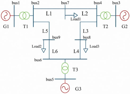
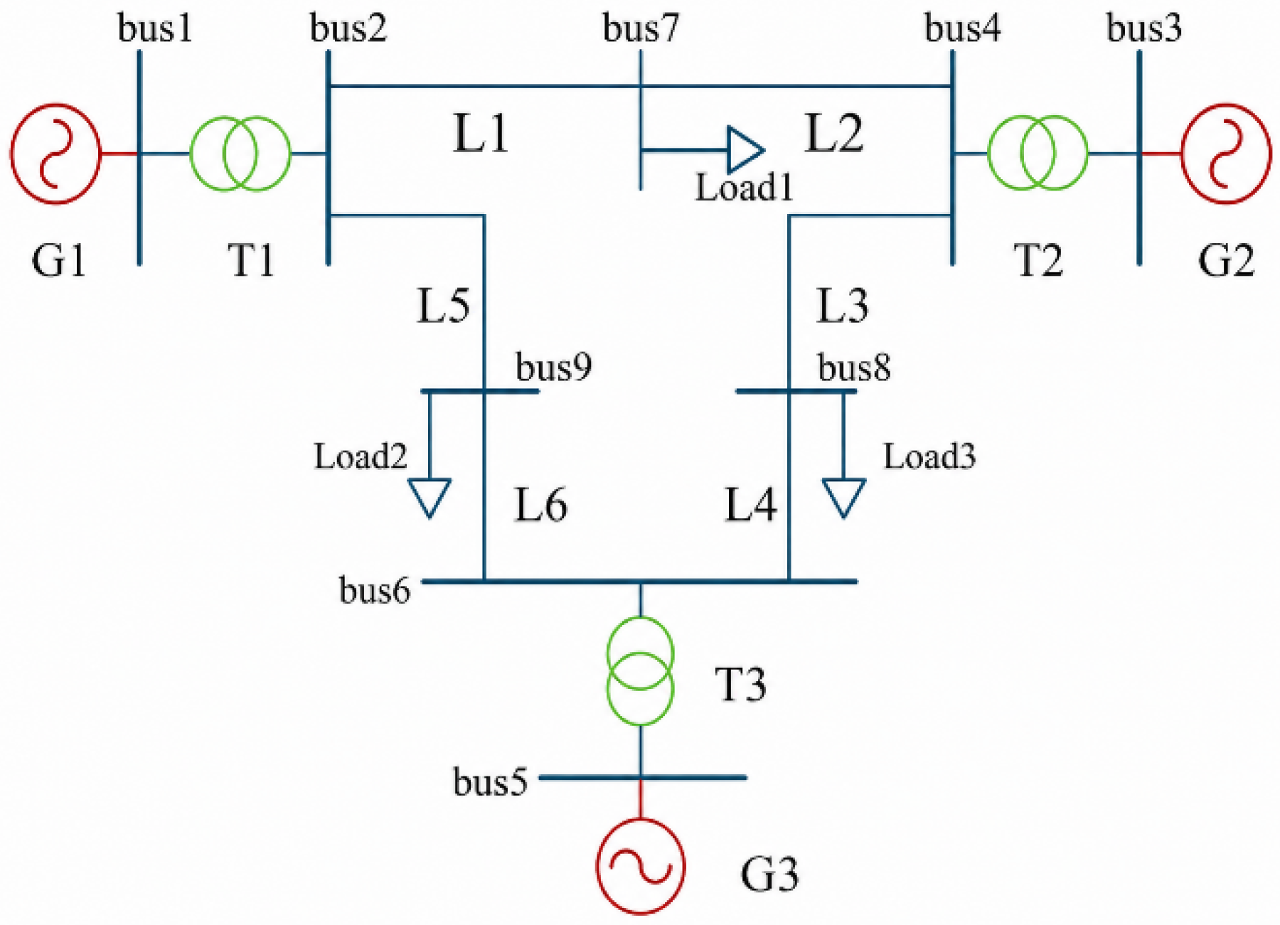
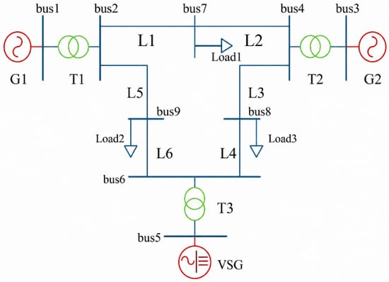
The method was first evaluated on the network shown in Figure 2, which captures the propagation of frequency dynamics in a system with multiple generators, loads, and disturbance locations. The rated voltage, installed capacity, and connection bus of each generator are listed in Table 3. Generator inertia constants were varied randomly to examine the effects of nodal inertia on the frequency response, and comparative tests were conducted for different disturbance locations and magnitudes.

Figure 2. IEEE 3-machine 9-bus test system.

Table 3. Generator parameters of the IEEE 9-bus test system.

Generation Unit	Rated Voltage (kV)	Rated Capacity (MVA)	Local Load (kW)	Connection Bus
G1	18	200	10	1
G2	16.5	175	10	3
G3	13.8	230	10	5

To assess applicability to renewable generation, a renewable-integrated configuration of the 3-machine 9-bus system was also constructed, as shown in Figure 3. The original network topology, line configuration, and load buses were retained, while G3 was replaced by a converter-interfaced renewable generation unit controlled as a virtual synchronous generator (VSG). The control strategies of the other generators were unchanged. Selected VSG control parameters are listed in Table 4.

Figure 3. IEEE 3-machine 9-bus test system with grid-forming renewable generation.

Table 4. Parameters of the VSG-controlled renewable generation unit.

Parameter	Value
Active power reference Pref	0.40 p.u.
Virtual inertia constant Hvsg	1–20 s
Damping coefficient D	0.015 p.u.
Coupling inductance Lf	0.30 p.u.
Control sampling frequency fs	5 kHz
Power-tracking proportional gain Kp,track	4
Power-tracking integral gain Ki,track	6 s−1

To assess performance under different operating conditions, 1000 sensitivity tests were conducted on the system in Figure 2 and 200 on the system in Figure 3. Across these 1200 tests, generator inertia, line length, disturbance magnitude, and disturbance location were varied within the ranges listed in Table 5.

Table 5. Parameter ranges used in the simulation sweep.

System Parameter	Parameter Range
Generator inertia	1–20 s
Disturbance magnitude	1–8% of total system load (approximately 350 MW)
Line length	1–100 km
Disturbance location	Buses 7, 8, and 9

In each test, an active load disturbance was applied at a specified bus, and PMUs recorded the resulting nodal active power and frequency responses. The pre-disturbance steady-state means were used as baselines to construct the active power deviation ΔP and frequency deviation Δf. The signals ΔP and Δf were processed using a third-order Butterworth filter with a cutoff frequency of 0.5 Hz. All algorithms used the same frequency measurements and power-input signals to ensure a fair comparison.

The UKF, ARX-UKF, and IG-UKF were used as benchmarks. The comparison was designed to distinguish the contributions of the individual modules. The UKF and IG-UKF used the same manually specified initial inertia, whereas ARX-UKF and ARX-IG-UKF were initialized with the inertia estimate obtained from the ARX model. The same initial covariance parameters were used across the algorithms. This setup allowed the effects of ARX-based initialization on convergence and IG-based measurement noise adaptation on estimation accuracy to be assessed separately.

Absolute and relative errors were used to evaluate inertia estimation accuracy. For test m, the absolute error E_MAE and relative error E_MAPE between the true and estimated inertia were defined as

$$\left\{\begin{array}{c}{E}_{\mathit{MAE}}=\left|{\widehat{H}}_m-H_m\right|\\ E_{\mathit{MAPE}}={\displaystyle \frac{\left|{\widehat{H}}_m-H_m\right|}{H_m}}\times 100\%\end{array}\right.$$

(38)

4.2. Results Under Representative Operating Conditions

Tests were conducted on both the all-synchronous system in Figure 2 and the renewable-integrated system in Figure 3 to compare nodal inertia estimation under representative disturbances and assess applicability to different generation types. To limit the effects of disturbance magnitude, line parameters, and disturbance location, both systems were tested under fixed disturbance conditions. A load disturbance equal to 3% of the total system load was applied at bus 7. The proposed ARX-IG-UKF was compared with the UKF, ARX-UKF, and IG-UKF.

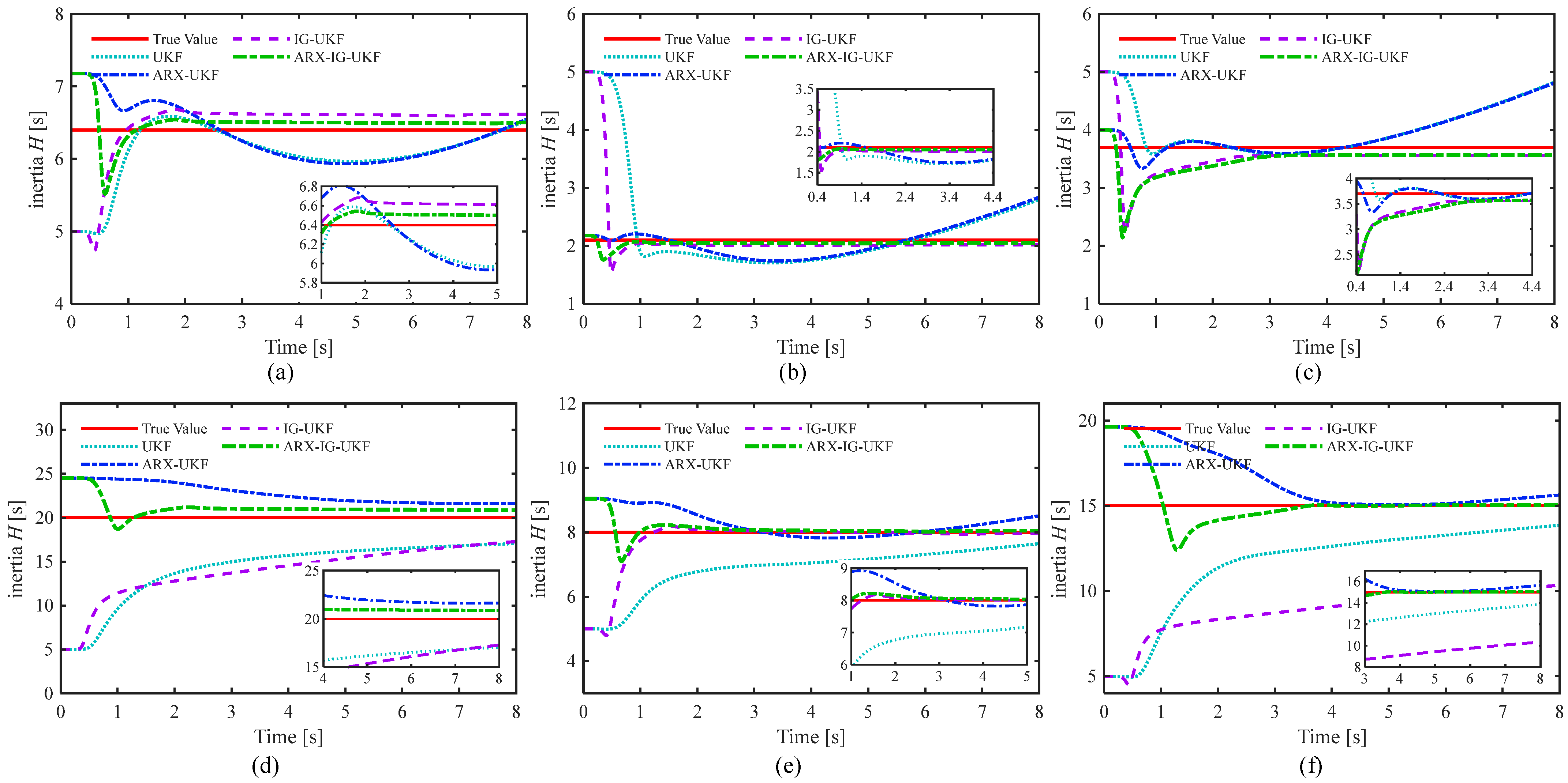
Two groups of tests were first conducted on the all-synchronous system. In Group 1, the true inertia constants of G1, G2, and G3 were set to 6.4, 2.1, and 3.7 s, respectively. In Group 2, they were set to 20, 8, and 15 s to examine convergence and estimation stability when the true inertia differed substantially from the initial filter value. The results are shown in Figure 4. For a fair comparison, the initial inertia was set to 5 s for both the UKF and IG-UKF.

Figure 4. Inertia estimates for the all-synchronous system: (a–c) G1, G2, and G3 in Group 1, respectively; (d–f) G1, G2, and G3 in Group 2, respectively.

The results for Group 1 are shown in Figure 4a–c. Both IG-UKF and ARX-IG-UKF converge rapidly to values close to the true inertia, with similar accuracy and a slight advantage for ARX-IG-UKF. When the manually specified initial value H₀ = 5 s is relatively close to the true inertia, initialization error is not the dominant limitation, and adaptive measurement noise updating provides a more evident improvement. By contrast, the UKF and ARX-UKF use a fixed measurement noise covariance and cannot adjust the correction weight according to the frequency-measurement residual. As the estimation window extends and primary frequency regulation and other unmodeled dynamics become more pronounced, these fixed-noise methods may continue to update the inertia state using frequency information no longer dominated by the inertial response, causing the estimates to depart from the true values.

The results for Group 2 are shown in Figure 4d–f. The accuracy of IG-UKF decreases markedly when the true inertia differs substantially from the specified initial value. Although IG-UKF adapts the measurement noise covariance, its initial inertia is still set manually. Because the information relevant to inertia identification is concentrated in the early disturbance response, a large initialization error may prevent the filter from converging within the limited inertial response window. ARX-UKF and ARX-IG-UKF instead obtain more appropriate initial inertia values from the ARX model and therefore perform better in this group of tests.

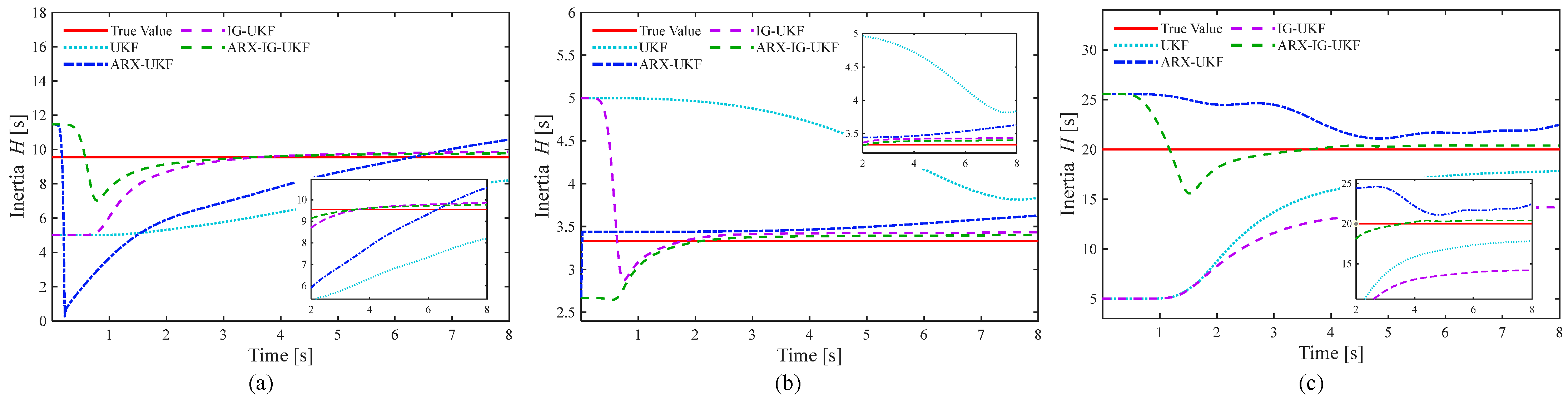
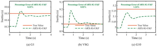
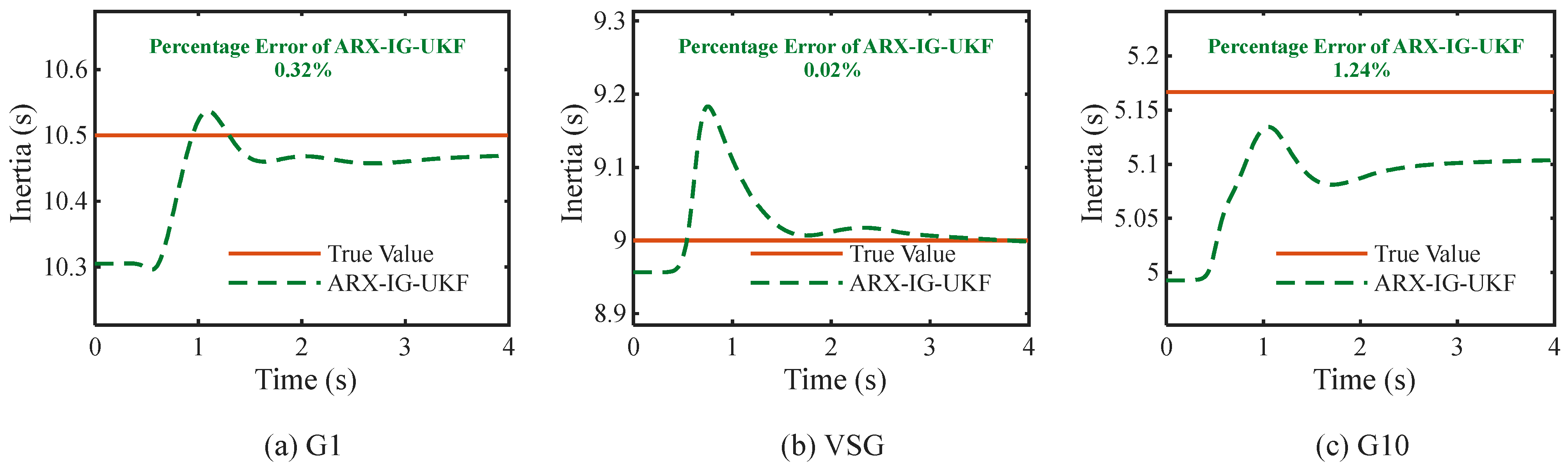
The ability to identify the virtual inertia of converter-interfaced renewable generation was further examined in the 3-machine 9-bus system with grid-forming renewable generation. The true inertia constants of G1, G2, and the VSG were set to 9.55, 3.33, and 20 s, respectively. The inertia estimation trajectories are shown in Figure 5.

Figure 5. Inertia estimates for the renewable-integrated system: (a) G1; (b) G2; (c) VSG.

As shown in Figure 5, the overall convergence behavior of the algorithms after introducing the VSG remains consistent with that observed in the two all-synchronous test groups. The proposed method estimates the VSG inertia with a relative error of 1.96%, indicating that it retains high accuracy for converter-interfaced renewable generation.

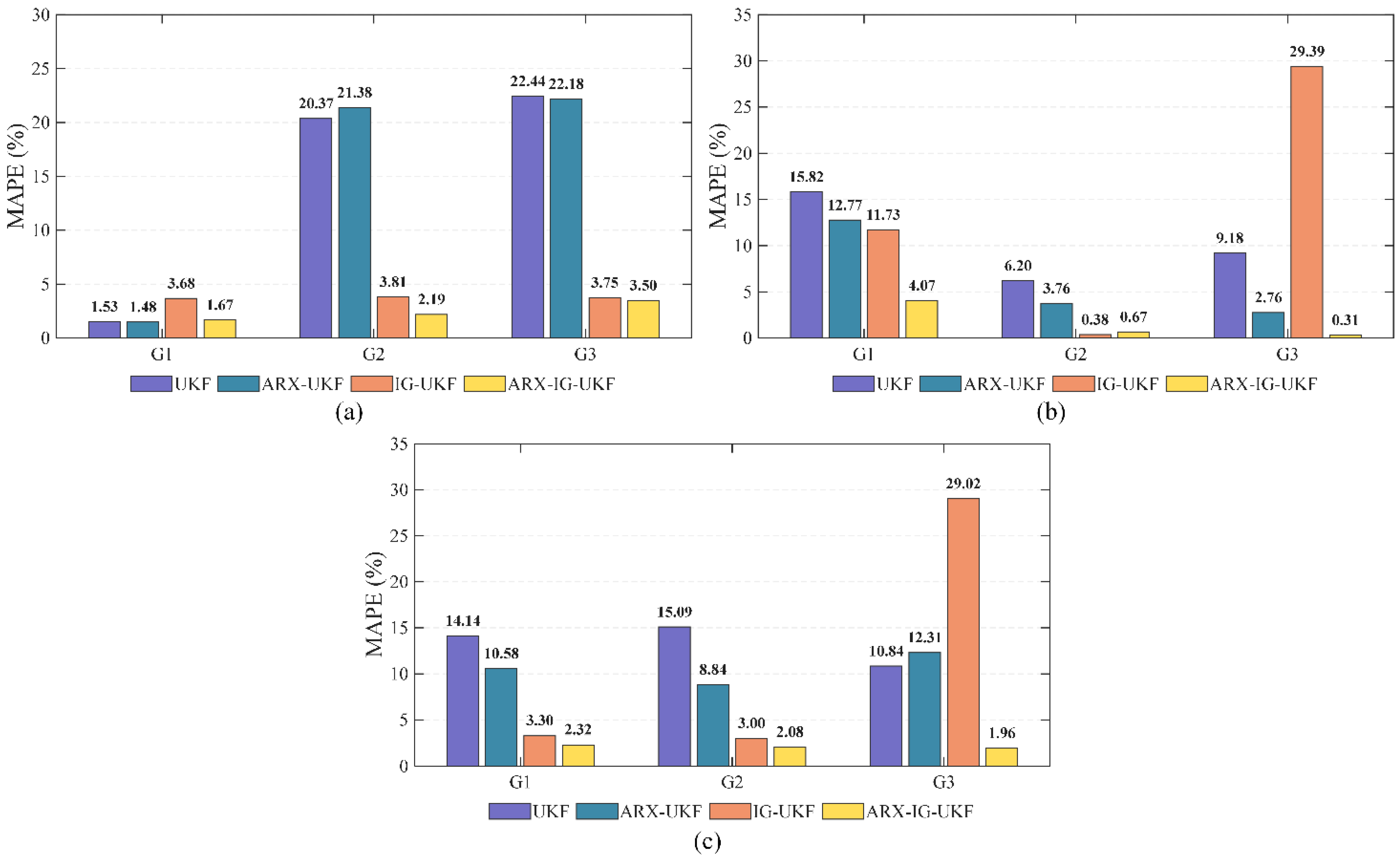
Together, the three test groups show that ARX-IG-UKF combines the benefits of ARX-based initialization and IG-based measurement noise adaptation. It reduces sensitivity to the initial state while limiting the late-stage estimation drift associated with a fixed measurement noise covariance, providing consistent convergence and stable estimates across different inertia levels. The estimation accuracy for the three test groups is summarized in Figure 6.

Figure 6. Inertia estimation errors for the three representative test groups: (a) Group 1; (b) Group 2; (c) Group 3.

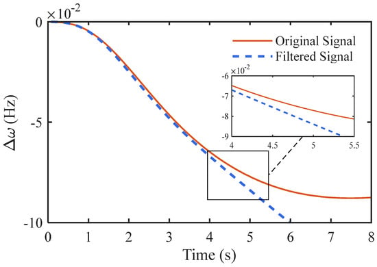
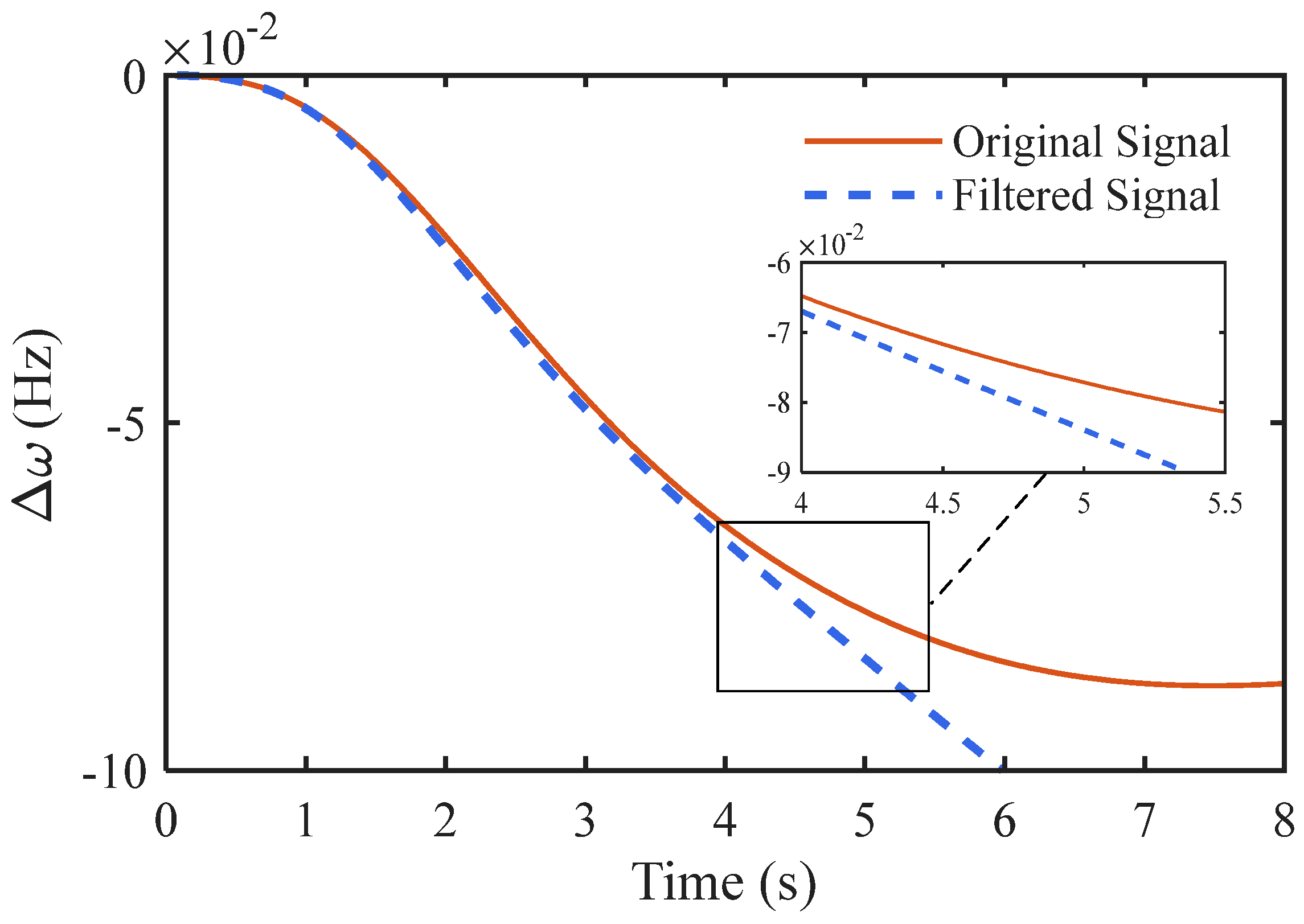
To further examine the behavior of the proposed method, one test was selected at random to compare the original and filtered frequency signals, as shown in Figure 7. Immediately after the disturbance, the frequency dynamics are governed mainly by the active power imbalance and system inertia, consistent with the inertial response state equation. The measurement residual is therefore small, and the filtered frequency closely follows the original signal. As primary frequency regulation, load-frequency damping, and other control modes begin to contribute, the original trajectory departs from the pure inertial response model. The increasing residual causes IG-UKF to raise the equivalent measurement noise variance and reduce the influence of subsequent frequency measurements on the state update. The filter thus no longer forces the model to follow the original frequency signal containing non-inertial dynamics. Instead, it retains the dominant response relevant to inertia estimation, limiting interference from other dynamics in accordance with the intended design.

Figure 7. Frequency signal filtered by ARX-IG-UKF.

4.3. Statistical Performance Under Randomized Parameters

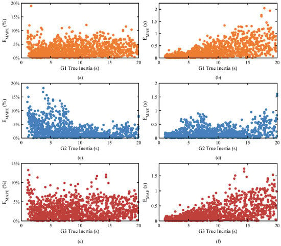
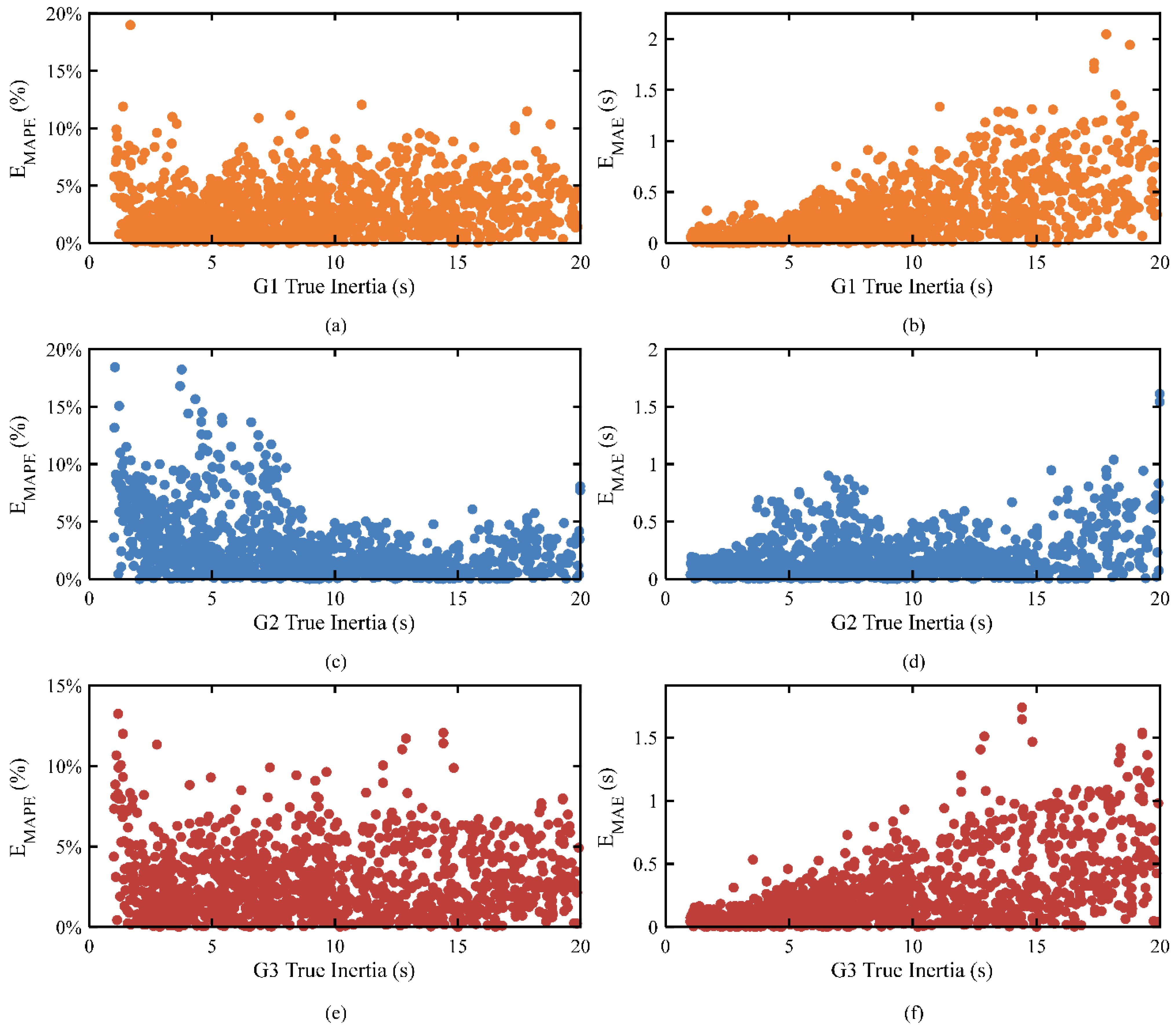
To assess the performance of ARX-IG-UKF under varying operating conditions, 1000 randomized tests were conducted on the all-synchronous system and 200 on the renewable-integrated system, using the parameter ranges in Section 4.1. Generator inertia, line length, disturbance magnitude, and disturbance location were randomly selected for each test. The proposed and benchmark methods were applied to estimate nodal inertia, and their absolute and relative errors were recorded. The ARX-IG-UKF results are shown in Figure 8. Table 6 summarizes the accuracy of all algorithms across the 1200 randomized tests. The mean relative error for the VSG across the 200 renewable-integrated tests was 3.21%, supporting the applicability of the method to systems with renewable generation.

Figure 8. Inertia estimation errors across randomized operating conditions: (a) MAPE of G1; (b) MAE of G1; (c) MAPE of G2; (d) MAE of G2; (e) MAPE of G3; (f) MAE of G3.

Table 6. MAPE and MAE across randomized operating conditions.

Generator Unit	Algorithm	MAPE(%)	MAE(s)
G1	UKF	21.7364	1.4264
	ARX-UKF	14.2594	0.8459
	IG-UKF	8.2512	1.1845
	ARX-IG-UKF	3.0858	0.2988
G2	UKF	30.0401	1.8206
	ARX-UKF	19.6262	1.1982
	IG-UKF	9.3503	1.6602
	ARX-IG-UKF	2.7337	0.1877
G3	UKF	11.6350	1.1444
	ARX-UKF	9.1547	0.4805
	IG-UKF	10.5342	2.0027
	ARX-IG-UKF	2.7555	0.2779

Figure 8 shows the distributions of relative and absolute errors at different inertia levels. For all three generators, most estimates have small errors, indicating consistent performance across the tested inertia range. Relative errors vary more noticeably for some low-inertia cases, where the faster post-disturbance frequency changes make measurement noise, filtering errors, and transient dynamics more influential. As inertia increases, the relative-error distribution generally narrows, suggesting that the algorithm can accommodate the power frequency dynamics associated with different inertia levels.

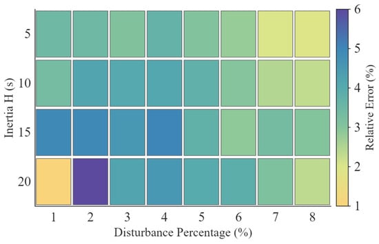
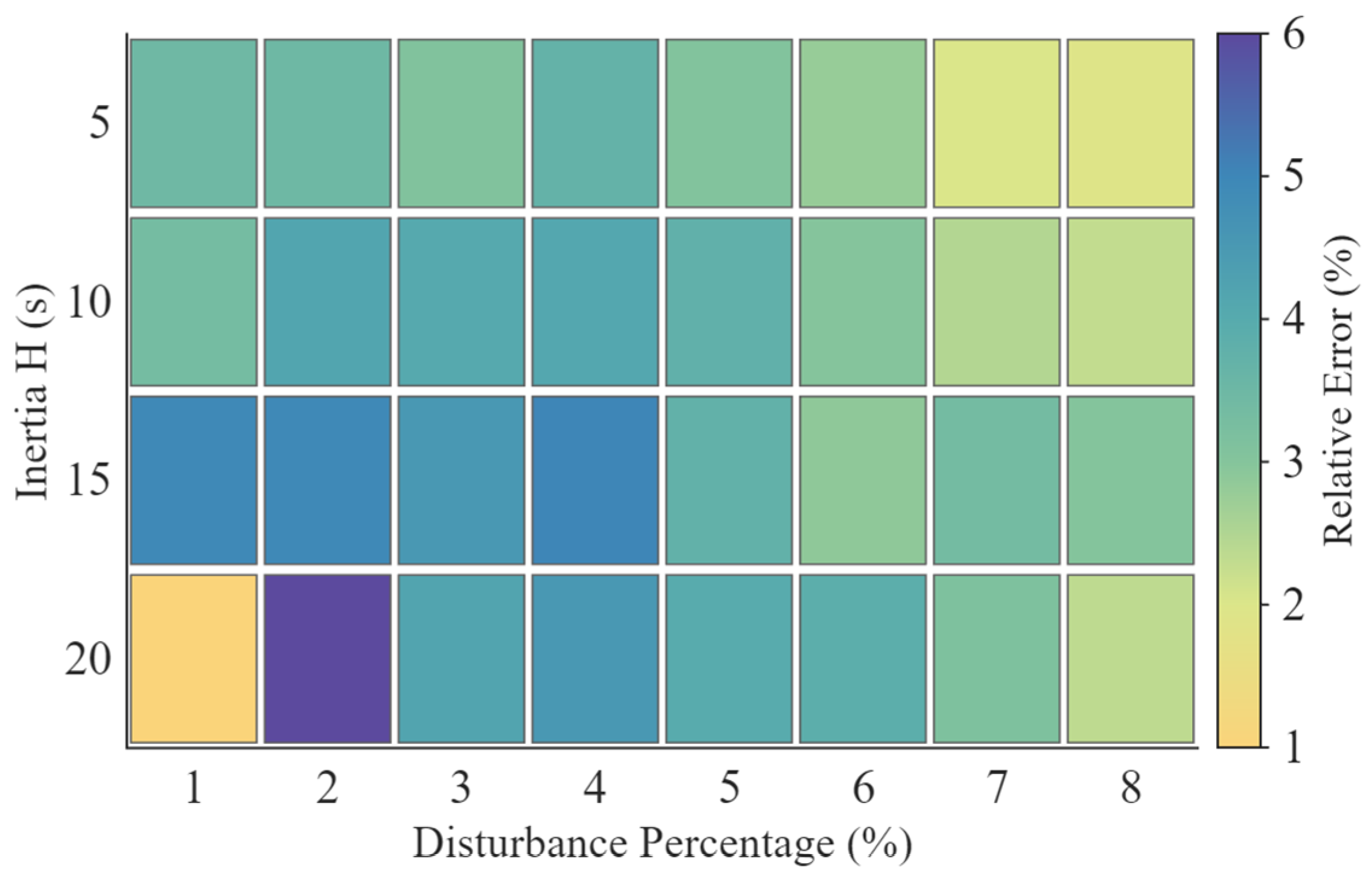
Figure 9 further illustrates how inertia estimation errors vary with disturbance magnitude and inertia. Relative errors generally decrease as the disturbance becomes larger because inertia-related characteristics become more prominent in the measured signals. At a fixed measurement noise level, a larger disturbance also increases the proportion of useful dynamic information, reducing the influence of local signal fluctuations on parameter estimation.

Figure 9. Relative inertia estimation errors for different disturbance magnitudes and inertia constants.

The relative errors generally decrease as inertia increases, whereas the spread of absolute errors tends to grow with the true inertia. Nevertheless, the absolute errors remain small for most tests, indicating stable estimation across different generator inertia levels.

The relative- and absolute-error results show some loss of accuracy in cases with very low or high inertia or complex transient responses. Overall, however, the errors remain concentrated within a narrow range, with mean relative errors of approximately 3% for the three generators. These results indicate that ARX-IG-UKF maintains high accuracy across variations in inertia, disturbances, and network parameters, supporting its applicability to complex operating conditions.

4.4. Extended Tests Under Different Disturbance Types

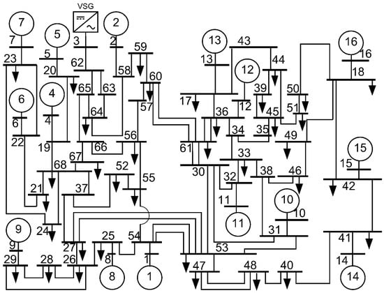
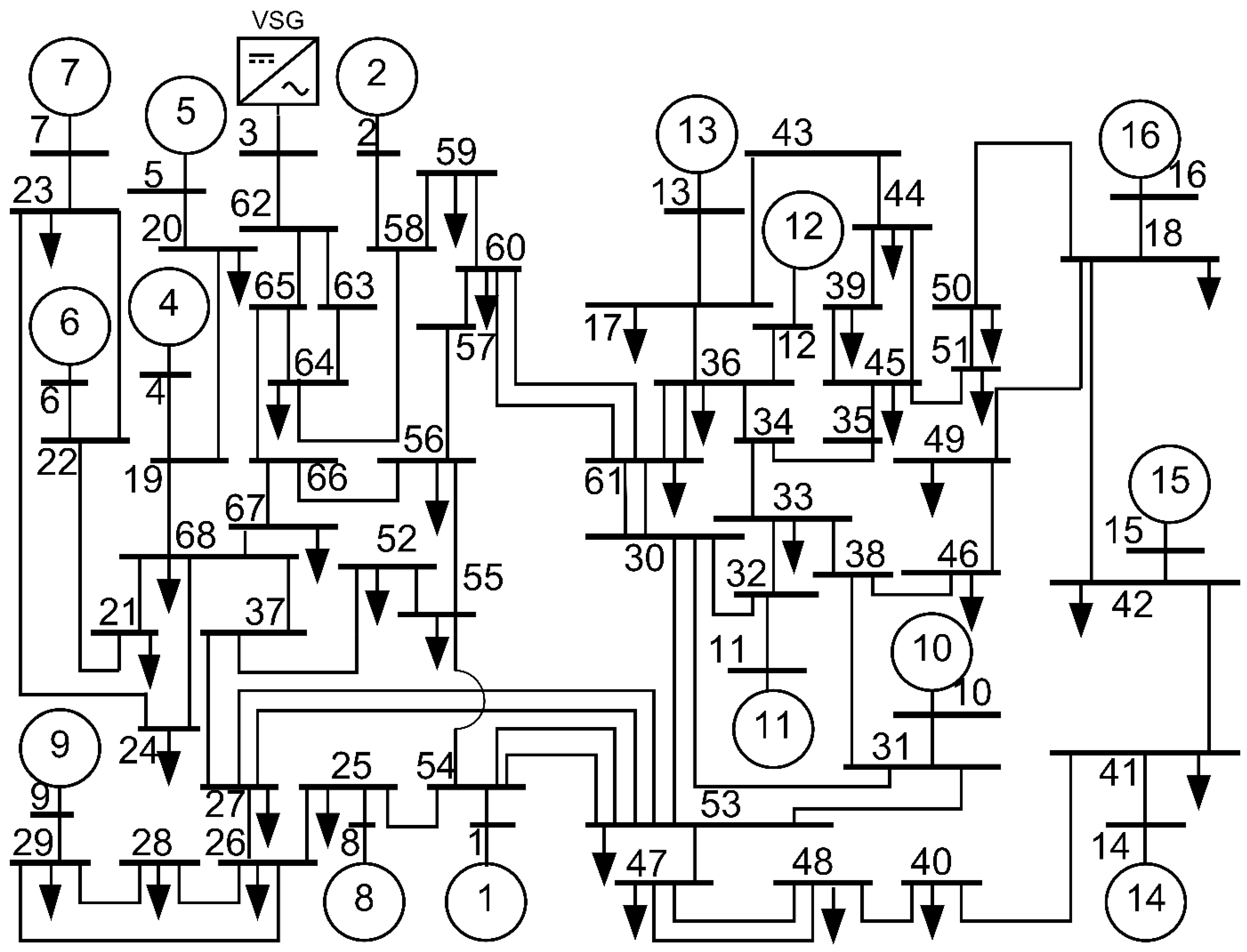
Following the tests on the 3-machine 9-bus system, further simulations were conducted on the IEEE 16-machine 68-bus system with grid-forming renewable generation to assess the applicability of ARX-IG-UKF to a larger network, more complex interactions among generators, and different disturbance types. The system is shown in Figure 10. Synchronous generator G3 was replaced by a converter-interfaced renewable generation unit using VSG control.

Figure 10. IEEE 16-machine 68-bus system with renewable generation.

To avoid limiting the evaluation to a single type of step disturbance, four scenarios with different dynamic characteristics were considered: a load step, a three-phase short circuit, a synchronous-generator trip, and a change in renewable active power output. The test conditions were as follows:

• Load step: A step load of 176.207 MW and 17.6207 Mvar was connected at bus 49 during the simulation.
• Three-phase short circuit: A temporary three-phase fault was applied at the bus 29 end of the bus 29-bus 26 line and cleared after 0.1 s.
• Generator trip: After the system reached steady state, the circuit breaker of G1 was opened to disconnect the generator. G1 had a rated capacity of 400 MVA and a pre-trip active power output of approximately 250 MW.
• Renewable power-output variation: A time-varying active power reference was applied to the VSG-controlled renewable generation unit to simulate a rapid output change. Before the disturbance, the system operated in steady state, and G3 generated approximately 650 MW. Instead of an ideal step input, a smooth cosine-shaped reduction in the active power reference was applied from the disturbance onset. The output fell to 40% of its pre-disturbance value within 2 s and returned to that value over the following 2 s.

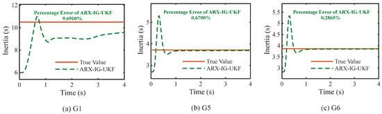
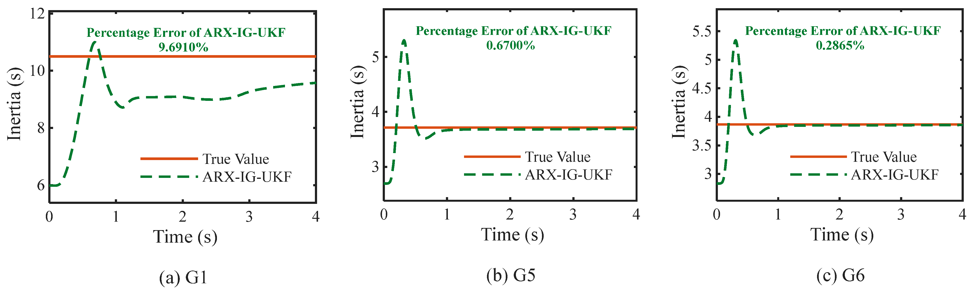
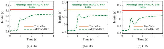
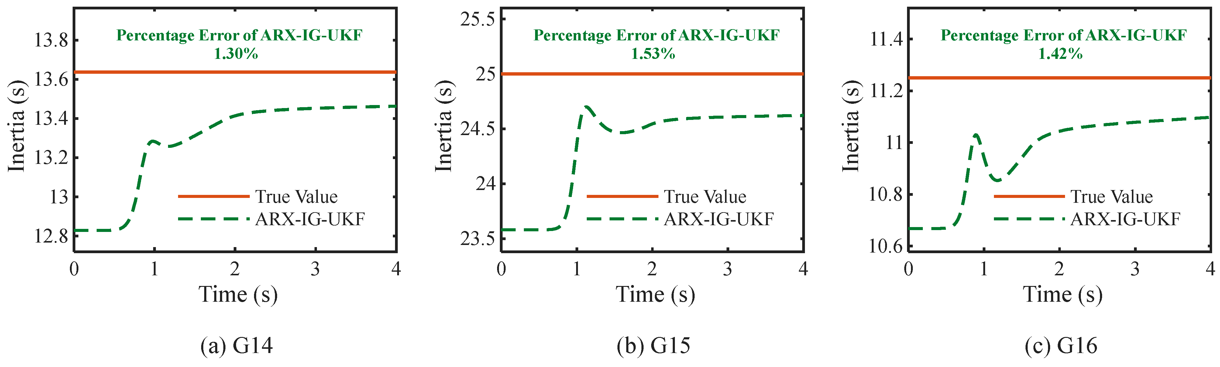
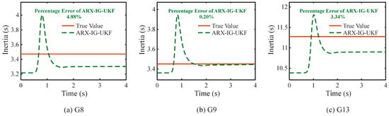
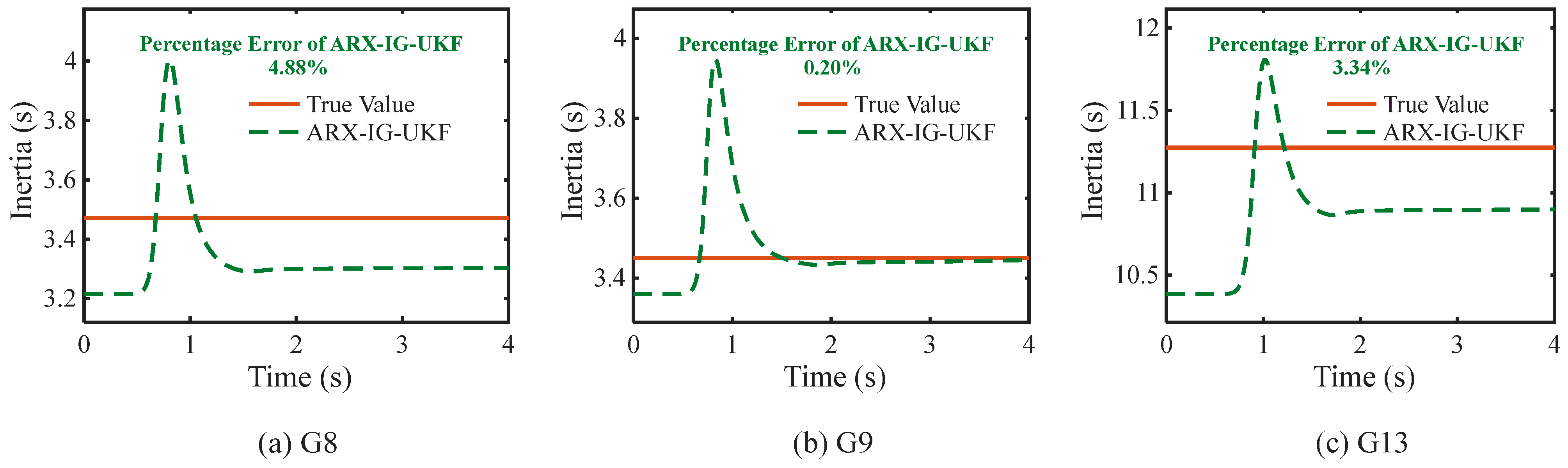
The relative inertia estimation errors of the 16 generation units under the four disturbance scenarios are listed in Table 7. Three units were randomly selected for each scenario, and their estimation results are shown in Figure 11, Figure 12, Figure 13 and Figure 14.

Table 7. Relative inertia estimation errors (%) under four disturbance scenarios.

Generation Unit	True Inertia H (s)	Case 1: Load Step	Case 2: Three-Phase Short Circuit	Case 3: Generator Trip	Case 4: Renewable Output Variation
G1	10.5000	0.3163	9.6910	--	1.0782
G2	4.3143	0.8260	2.8741	0.0549	11.6030
VSG	9.0000	0.0165	0.4128	0.5223	0.2347
G4	3.5750	0.0618	3.2092	2.9453	2.7099
G5	3.7143	0.5633	0.6700	2.9953	3.6943
G6	3.8667	0.6260	0.2865	1.7202	3.3904
G7	3.3000	0.7328	3.7618	2.5137	4.4691
G8	3.4714	1.0913	1.8594	20.3241	4.8788
G9	3.4500	3.0375	--	2.8438	0.1992
G10	5.1667	1.2351	3.6258	0.8850	2.6473
G11	2.3500	3.7112	16.4517	6.3913	6.6092
G12	5.4294	3.2321	7.1058	0.1866	5.0541
G13	11.2727	1.6700	2.2250	1.3176	3.3356
G14	13.6364	1.4655	3.3277	1.3021	1.0446
G15	25.0000	1.2601	2.7443	1.5304	1.8181
G16	11.2500	2.4413	3.5423	1.4194	0.8056
Mean APE (%)	--	1.3929	4.1192	3.1301	3.3483

Figure 11. Inertia estimation results for Case 1 (load step).

Figure 12. Inertia estimation results for Case 2 (three-phase short circuit).

Figure 13. Inertia estimation results for Case 3 (generator trip).

Figure 14. Inertia estimation results for Case 4 (renewable power-output variation).

The disturbance type affects estimation accuracy to varying degrees, but the method provides stable inertia estimates for most units and scenarios. The mean relative errors for the four cases were 1.3929%, 4.1192%, 3.1301%, and 3.3483%, respectively, indicating that the method scales effectively to the renewable-integrated IEEE 16-machine 68-bus system. The VSG-controlled renewable unit maintained low relative errors in all four cases, demonstrating effective identification of its virtual inertia.

The load-step case gave the best results, with a mean relative error of 1.3929% and relative errors below 5% for every unit. The three-phase short-circuit case produced the largest mean relative error. A short circuit introduces strong, fast electromagnetic transients and pronounced local frequency dynamics, causing the early power-frequency response to depart from an inertia-dominated relationship. G9 was identified as a near-fault unit using a fault-proximity detection procedure based on [28,29]. Previous inertia estimation studies have shown that faults close to a generator cause greater distortion of local measurements. The approximate relationship between rotor speed and terminal-bus frequency used for inertia estimation may then break down, making estimates based on terminal frequency unreliable [30]. The G9 measurements in the short-circuit case were therefore excluded from inertia estimation. A small number of units also exhibited relatively large errors in the short-circuit, generator-trip, and renewable-output-variation cases. Future work will examine electrical distance, local dynamic modes, and the observability of power-frequency measurements to clarify the causes of these larger nodal errors and identify possible improvements.

4.5. Robustness Analysis

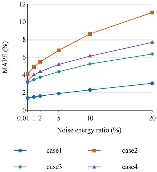
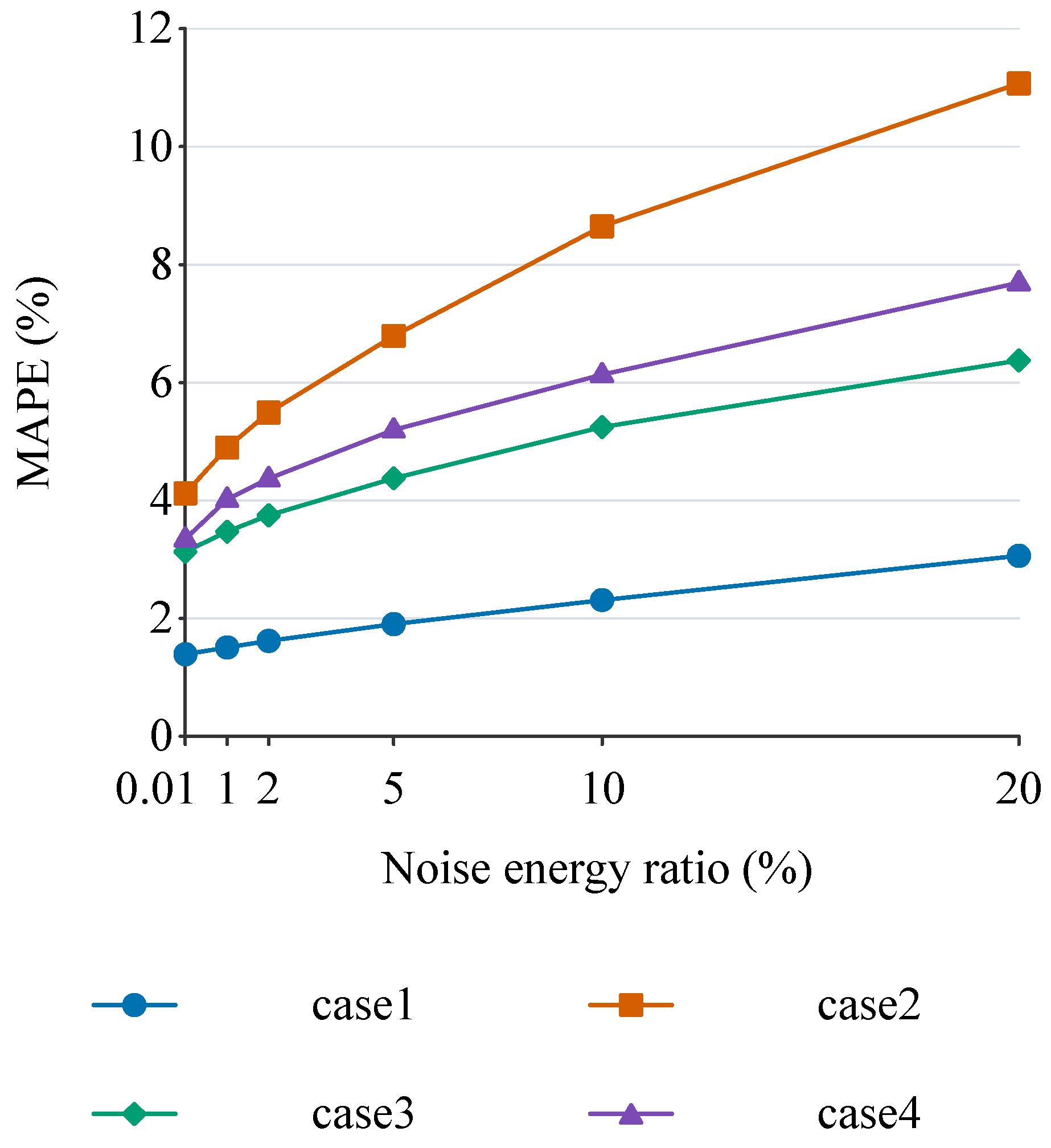
Robustness to increasing measurement noise was evaluated on the IEEE 16-machine 68-bus system with grid-forming renewable generation under all four disturbance scenarios. Using the noise energy ratio r defined in Section 4.1, the noise levels were set to 0.01%, 1%, 2%, 5%, 10%, and 20%. The results are plotted in Figure 15, with the numerical values reported in Table 8.

Figure 15. Inertia estimation performance at different noise levels.

Table 8. Mean relative inertia estimation errors (%) at different noise levels.

Noise Energy Ratio (%)	Case 1	Case 2	Case 3	Case 4
0.01	1.3929	4.1192	3.1301	3.3483
1	1.5093	4.8976	3.4709	4.0207
2	1.6203	5.4912	3.7484	4.3690
5	1.9022	6.7905	4.3786	5.1950
10	2.3111	8.6500	5.2442	6.1330
20	3.0614	11.0738	6.3760	7.6921

Figure 15 shows the variation in inertia estimation errors with Gaussian white-noise level for the four disturbance scenarios. ARX-IG-UKF retains a degree of noise tolerance across the tested levels and provides relatively stable accuracy under low-to-moderate noise conditions.

The mean relative error increases with the noise energy ratio in all four cases, although the rate of increase differs appreciably among disturbance types. The load-step case consistently produces the lowest error and is the least sensitive to increasing noise. Even at a noise energy ratio of 20%, its mean relative error remains approximately 3%, indicating good noise tolerance for this disturbance. By contrast, the short-circuit case has the largest errors and the most pronounced increase with noise level. The generator-trip and renewable-output-variation cases lie between these extremes, showing that sensitivity to measurement noise depends on the disturbance dynamics.

Additional tests were conducted to assess robustness to anomalous PMU measurements. Building on the Gaussian white-noise tests, the load-step and three-phase short-circuit cases were selected for tests involving outliers and missing data. Spike outliers with amplitudes of 0.1–0.5 Hz were added to randomly selected frequency measurements, affecting 5% of the samples. Missing-data conditions included a 5% random sample-loss rate and interruptions lasting one or three consecutive samples, representing random data loss and brief measurement outages.

The mean relative errors for the two disturbance scenarios were compared with those obtained without measurement anomalies. The results are given in Table 9.

Table 9. Mean relative inertia estimation errors (%) with and without PMU measurement anomalies.

Measurement Condition	Case 1	Case 2
Measurements without Anomalies	1.9588	6.8371
Combined PMU Measurement Anomalies	1.8578	6.8390

As shown in Table 9, the proposed method remains capable of estimating inertia in the presence of PMU measurement anomalies, although performance depends on the disturbance scenario. The mean relative errors change only slightly in both the load-step and short-circuit cases. Overall, the method tolerates the tested PMU anomalies, but its robustness remains dependent on the disturbance type.

5. Conclusions

This paper formulates a state-space model linking the nodal inertia constant with frequency dynamics by combining the inertial response characteristics of conventional synchronous generators and renewable generation units. An ARX-IG-UKF-based method is then developed for nodal inertia estimation. The ARX model provides an initial nodal inertia estimate, reducing the constraint imposed by the limited convergence rate of the Kalman filter during short-window identification. The inverse-gamma distribution is used to adapt the measurement noise variance, limiting the effects of frequency-measurement errors and unmodeled dynamics. The simulation results support the following conclusions:

• ARX-based initialization provides the UKF with a more appropriate initial state and shortens the time required for the inertia estimate to approach the true value. The recursive estimate, therefore, enters its effective range earlier within the finite inertial response window. This reduces convergence delay when the initial inertia error is large and improves estimation stability and robustness.
• Adaptive updating of the measurement noise variance using an inverse-gamma distribution allows the UKF to adjust the measurement-correction weight according to the frequency residual. This reduces interference from primary frequency regulation and other unmodeled dynamics, improving inertia estimation accuracy. Across the 1200 randomized scenarios, ARX-IG-UKF outperformed the UKF, ARX-UKF, and IG-UKF in relative-error metrics and also achieved favorable absolute errors. These results demonstrate its overall effectiveness under the parameter variations considered in this study.

References

- Eltohamy, M.S.; Hassanin, M.A.; Khodeir, N.A.; Alsayed, Y.M.; Awad, F.H.; Hassan, A.Y.; Sotouhy, M.M.E.; Mansour, A.M.; Khater, F.M.H. Artificial intelligence–enabled energy interconnection for low-carbon power systems and electric mobility: A comparative review of China and Egypt. Glob. Energy Interconnect. 2026; in press. [CrossRef] [Scilit]
- Hatziargyriou, N.; Milanovic, J.; Rahmann, C.; Ajjarapu, V.; Canizares, C.; Erlich, I.; Hill, D.; Hiskens, I.; Kamwa, I.; Pal, B.; et al. Definition and Classification of Power System Stability—Revisited & Extended. IEEE Trans. Power Syst. 2021, 36, 3271–3281. [Google Scholar] [CrossRef] [Scilit]
- Breyer, C.; Khalili, S.; Bogdanov, D.; Ram, M.; Oyewo, A.S.; Aghahosseini, A.; Gulagi, A.; Solomon, A.A.; Keiner, D.; Lopez, G.; et al. On the History and Future of 100% Renewable Energy Systems Research. IEEE Access 2022, 10, 78176–78218. [Google Scholar] [CrossRef] [Scilit]
- Tan, B.; Zhao, J.; Netto, M.; Krishnan, V.; Terzija, V.; Zhang, Y. Power system inertia estimation: Review of methods and the impacts of converter-interfaced generations. Int. J. Electr. Power Energy Syst. 2022, 134, 107362. [Google Scholar] [CrossRef] [Scilit]
- Heylen, E.; Teng, F.; Strbac, G. Challenges and opportunities of inertia estimation and forecasting in low-inertia power systems. Renew. Sustain. Energ. Rev. 2021, 147, 111176. [Google Scholar] [CrossRef] [Scilit]
- Tan, B.; Zhao, J. Data-Driven Adaptive Unscented Kalman Filter for Time-varying Inertia and Damping Estimation of Utility-scale IBRs Considering Current Limiter. IEEE Trans. Power Syst. 2024, 39, 7331–7345. [Google Scholar] [CrossRef] [Scilit]
- Wu, Y.K.; Yang, W.H.; Hu, Y.L.; Dzung, P.Q. Frequency Regulation at a Wind Farm Using Time-Varying Inertia and Droop Controls. IEEE Trans. Ind. Appl. 2019, 55, 213–224. [Google Scholar] [CrossRef] [Scilit]
- Bizzarri, F.; Giudice, D.D.; Grillo, S.; Linaro, D.; Brambilla, A.; Milano, F. Inertia Estimation Through Covariance Matrix. IEEE Trans. Power Syst. 2024, 39, 947–956. [Google Scholar] [CrossRef] [Scilit]
- Cao, X.; Stephen, B.; Abdulhadi, I.F.; Booth, C.D.; Burt, G.M. Switching Markov Gaussian Models for Dynamic Power System Inertia Estimation. IEEE Trans. Power Syst. 2016, 31, 3394–3403. [Google Scholar] [CrossRef] [Scilit]
- Zeng, F.; Zhang, J.; Zhou, Y.; Qu, S. Online Identification of Inertia Distribution in Normal Operating Power System. IEEE Trans. Power Syst. 2020, 35, 3301–3304. [Google Scholar] [CrossRef] [Scilit]
- Tuttelberg, K.; Kilter, J.; Wilson, D.; Uhlen, K. Estimation of Power System Inertia From Ambient Wide Area Measurements. IEEE Trans. Power Syst. 2018, 33, 7249–7257. [Google Scholar] [CrossRef] [Scilit]
- Yang, D.; Wang, B.; Cai, G.; Chen, Z.; Ma, J.; Sun, Z.; Wang, L. Data-Driven Estimation of Inertia for Multiarea Interconnected Power Systems Using Dynamic Mode Decomposition. IEEE Trans. Ind. Inform. 2021, 17, 2686–2695. [Google Scholar] [CrossRef] [Scilit]
- Li, Y.; Yao, W.; Zhao, Y.; Huang, W.; Zhai, S.; Li, W.; Wen, J.; Xia, Y. Real-time estimation of time-varying inertia for non-synchronous devices using streaming dynamic mode decomposition. Int. J. Electr. Power Energy Syst. 2024, 157, 109847. [Google Scholar] [CrossRef] [Scilit]
- Mohagheghi, S.; Alaileh, R.H.; Cokkinides, G.; Meliopoulos, A.P.S. Distributed state estimation based on the supercalibrator concept—Laboratory implementation. In Proceedings of the 2007 iREP Symposium—Bulk Power System Dynamics and Control—VII. Revitalizing Operational Reliability, Charleston, SC, USA, 19–24 August 2007. [Google Scholar]
- Ghahremani, E.; Kamwa, I. Dynamic State Estimation in Power System by Applying the Extended Kalman Filter With Unknown Inputs to Phasor Measurements. IEEE Trans. Power Syst. 2011, 26, 2556–2566. [Google Scholar] [CrossRef] [Scilit]
- Ghahremani, E.; Kamwa, I. Online State Estimation of a Synchronous Generator Using Unscented Kalman Filter From Phasor Measurements Units. IEEE Trans. Energy Convers. 2011, 26, 1099–1108. [Google Scholar] [CrossRef] [Scilit]
- Fan, L.; Wehbe, Y. Extended Kalman filtering based real-time dynamic state and parameter estimation using PMU data. Electr. Power Syst. Res. 2013, 103, 168–177. [Google Scholar] [CrossRef] [Scilit]
- Tan, B.; Zhao, J. Data-Driven Time-Varying Inertia Estimation of Inverter-Based Resources. IEEE Trans. Power Syst. 2023, 38, 1795–1798. [Google Scholar] [CrossRef] [Scilit]
- Guo, J.; Wang, X.; Ooi, B.T. Estimation of Inertia for Synchronous and Non-Synchronous Generators Based on Ambient Measurements. IEEE Trans. Power Syst. 2022, 37, 3747–3757. [Google Scholar] [CrossRef] [Scilit]
- Fang, J.; Li, H.; Tang, Y.; Blaabjerg, F. On the Inertia of Future More-Electronics Power Systems. IEEE J. Emerg. Sel. Top. Power Electron. 2019, 7, 2130–2146. [Google Scholar] [CrossRef] [Scilit]
- Pulgar-Painemal, H.; Wang, Y.; Silva-Saravia, H. On Inertia Distribution, Inter-Area Oscillations and Location of Electronically-Interfaced Resources. IEEE Trans. Power Syst. 2018, 33, 995–1003. [Google Scholar] [CrossRef] [Scilit]
- Linaro, D.; Bizzarri, F.; Giudice, D.D.; Pisani, C.; Giannuzzi, G.M.; Grillo, S.; Brambilla, A.M. Continuous estimation of power system inertia using convolutional neural networks. Nat. Commun. 2023, 14, 4440. [Google Scholar] [CrossRef] [Scilit] [PubMed]
- Zhong, Q.C.; Weiss, G. Synchronverters: Inverters That Mimic Synchronous Generators. IEEE Trans. Ind. Electron. 2011, 58, 1259–1267. [Google Scholar] [CrossRef] [Scilit]
- Zhang, Y.; Melin, A.M.; Djouadi, S.M.; Olama, M.M.; Tomsovic, K. Provision for Guaranteed Inertial Response in Diesel-Wind Systems via Model Reference Control. IEEE Trans. Power Syst. 2018, 33, 6557–6568. [Google Scholar] [CrossRef] [Scilit]
- Bhui, P.; Senroy, N.; Singh, A.K.; Pal, B.C. Estimation of Inherent Governor Dead-Band and Regulation Using Unscented Kalman Filter. IEEE Trans. Power Syst. 2018, 33, 3546–3558. [Google Scholar] [CrossRef] [Scilit]
- Schiffer, J.; Aristidou, P.; Ortega, R. Online Estimation of Power System Inertia Using Dynamic Regressor Extension and Mixing. IEEE Trans. Power Syst. 2019, 34, 4993–5001. [Google Scholar] [CrossRef] [Scilit]
- Bai, Y.; Yan, B.; Zhou, C.; Su, T.; Jin, X. State of art on state estimation: Kalman filter driven by machine learning. Annu. Rev. Control 2023, 56, 100909. [Google Scholar] [CrossRef] [Scilit]
- Iii, E.O.S.; Roberts, J. Distance Relay Element Design. SEL J. Reliab. Power 2010, 1, 1–26. [Google Scholar] [CrossRef] [Scilit]
- Costello, D.; Moon, M.; Bow, G. Use of Directional Elements at the Utility-Industrial Interface. In Proceedings of the 2006 Power Systems Conference: Advanced Metering, Protection, Control, Communication, and Distributed Resources, Clemson, SC, USA, 14–17 March 2006; pp. 1–16. [Google Scholar]
- Tan, B.; Zhao, J.; Terzija, V.; Zhang, Y. Decentralized data-driven estimation of generator rotor speed and inertia constant based on adaptive unscented Kalman filter. Int. J. Electr. Power Energy Syst. 2022, 137, 107853. [Google Scholar] [CrossRef] [Scilit]
Disclaimer/Publisher’s Note: The statements, opinions and data contained in all publications are solely those of the individual author(s) and contributor(s) and not of MDPI and/or the editor(s). MDPI and/or the editor(s) disclaim responsibility for any injury to people or property resulting from any ideas, methods, instructions or products referred to in the content. |
© 2026 by the authors. Licensee MDPI, Basel, Switzerland. This article is an open access article distributed under the terms and conditions of the Creative Commons Attribution (CC BY) license.