CBF-QP Safety-Filter-Based Prescribed-Time Cooperative Guidance Under Deferred Field-of-View Constraints

Abstract

This paper addresses prescribed-time cooperative guidance of multiple fixed-wing unmanned aerial vehicles (UAVs) against a maneuvering aerial target in two-dimensional interception scenarios under onboard-seeker field-of-view (FOV) constraints. A deferred FOV mechanism is introduced to relax the boundary during the initial heading-adjustment phase and to recover the standard FOV limit after a user-selected delay. Prescribed-time disturbance observers estimate uncertainties caused by the target maneuver. Along the LOS direction, a prescribed-time cooperative guidance law is designed to achieve attack-time consensus. Meanwhile, a prescribed-time guidance law in the LOS-normal direction is developed to drive the LOS angular rate toward zero. A control-barrier-function quadratic program (CBF-QP) filter is then constructed to minimally modify the nominal prescribed-time acceleration commands while enforcing the deferred FOV constraint. Simulation results for three UAVs show the effectiveness of the proposed cooperative guidance scheme.

1. Introduction

Cooperative interception by multiple fixed-wing UAVs provides a means of concentrating sensing and control resources against a maneuvering aerial target while coordinating terminal conditions across spatially separated vehicles. In this setting, each UAV must generate compatible high-level guidance commands using local relative measurements and limited inter-UAV information, making distributed coordination essential [1,2]. Existing fixed-wing multi-UAV studies have established coordinated path-following under nominal and wind-disturbed conditions [3,4], constrained cooperative control [5,6], and formation regulation based on relative information [7]. Cooperative guidance is nevertheless challenging because attack-time coordination, target-maneuver compensation, seeker visibility, and feasible vehicle motion are strongly coupled. Rapid redistribution of the remaining flight time can demand large heading corrections. At the same time, the target must remain inside the onboard seeker FOV, and the coordination deadline must be met despite uncertain target acceleration.

FOV-constrained guidance has therefore received sustained attention. Representative approaches include look-angle shaping for impact-angle and time control [8]; two-stage cooperative guidance [9]; sliding-mode guidance for maneuvering targets [10]; three-dimensional FOV-constrained interception [11]; barrier-Lyapunov-function formulations for integrated guidance, bounded inputs, and prescribed-time coordination [12,13,14]; generalized three-dimensional or multiple-constraint designs [15,16]; and recent asymmetric barrier-Lyapunov-function formulations [17,18]. These studies demonstrate that seeker visibility should be treated as a state constraint rather than checked only after controller design. However, most methods impose the final FOV boundary throughout the engagement, which can make the initial geometry-adjustment phase unnecessarily restrictive. Target maneuvers introduce a second difficulty because unknown acceleration enters both radial and angular relative dynamics. Disturbance-observer-based control and active disturbance rejection provide systematic tools for estimating such lumped uncertainties [19,20]. Prescribed-time extended-state observers further make the reconstruction horizon assignable by design [21].

Convergence-time specification is another central issue in cooperative guidance. Finite-time and fixed-time cooperative guidance laws guarantee convergence within bounded horizons [22,23,24]. Related studies have further addressed delay-dependent stability [25] and fixed-time synchronization under complex or delayed interactions [26,27]. In contrast, prescribed-time control allows the designer to select the convergence deadline independently of initial conditions [28,29,30]. This property has been extended to multiagent consensus and containment [31], leader-following cluster consensus [32], prescribed-time pinning-group cooperative guidance [33], and related three-dimensional finite- and fixed-time cooperative guidance formulations [34,35]. For coordinated interception, an assignable deadline is valuable because disturbance reconstruction and attack-time consensus must be completed before the terminal phase. Existing results also indicate that convergence-time design must be coordinated across the observer and guidance channels rather than specified independently.

Control barrier functions (CBFs) offer a complementary mechanism for enforcing state constraints while retaining a nominal performance controller. The CBF-QP framework formulates safety as an online inequality constraint and minimally modifies the nominal command when the safe-set boundary is approached [36]. In cooperative UAV research, CBFs have been used for target search and tracking [37], collision avoidance in multi-fixed-wing pursuit–evasion [38], and collision avoidance and geofencing for fixed-wing aircraft [39]. Recent studies further discuss practical issues associated with input limits, disturbances, sampled-data implementation, output feedback, and reduced-order safety models [40,41]. For FOV-constrained cooperative guidance, this filtering structure is attractive because it can preserve a prescribed-time nominal law while correcting only the command component needed to maintain seeker visibility. Its integration with a deferred FOV boundary, two-channel prescribed-time guidance, and target-maneuver disturbance reconstruction remains a problem requiring a unified design.

These studies motivate the design of a cooperative guidance architecture that combines prescribed-time attack-time coordination, maneuver compensation, and explicit seeker constraints. Unlike [14], which integrates the barrier, controller, and observer in the LOS-frame law, the proposed method separates the nominal prescribed-time channels from a scalar CBF-QP filter and uses a deferred FOV boundary during initial geometry adjustment.

The main contributions are summarized as follows:

• A deferred FOV transformation is constructed to relax the initial constraint and recover the standard FOV boundary at the user-selected time.
• To address uncertainties caused by the target maneuver, prescribed-time disturbance observers are designed.
• Along the LOS direction, a prescribed-time cooperative guidance law is designed to achieve attack-time consensus. Meanwhile, a prescribed-time guidance law in the LOS-normal direction is developed to drive the LOS angular rate toward zero.
• A CBF-QP filter is constructed to minimally modify the nominal prescribed-time acceleration commands while enforcing the deferred FOV constraint.

2. Problem Formulation and Preliminaries

2.1. Engagement Geometry and Relative Dynamics

Consider N fixed-wing UAVs cooperatively intercepting a maneuvering aerial target in a two-dimensional inertial frame OXY. The pairs (x_i, y_i) and (x_T, y_T) denote the inertial coordinates of vehicle i and the target, respectively. For the i-th vehicle, let r_i denote the relative distance, q_i the line-of-sight angle measured from the positive X axis, v_i the vehicle speed, θ_i the vehicle heading angle, v_T the target speed, and θ_T the target heading angle. The relative kinematics are written as follows.

Each UAV and the target are modeled as planar point masses. The normal and tangential accelerations are high-level commands. This abstraction retains the translational geometry needed by the cooperative guidance design while leaving attitude, propulsion, actuator, and inner-loop tracking dynamics outside the present theoretical model. The sign conventions in the following equations are fixed by measuring both heading and LOS angles counterclockwise from the positive inertial axis:

$${\dot{r}}_i=v_T\cos ({\theta }_T-q_i)-v_i\cos ({\theta }_i-q_i)$$

(1)

$${\dot{q}}_i={\displaystyle \frac{v_T\sin ({\theta }_T-q_i)-v_i\sin ({\theta }_i-q_i)}{r_i}}$$

(2)

Equations (1) and (2) define the relative kinematics. The vehicle and target speed and heading dynamics are

$${\dot{\theta }}_i={\displaystyle \frac{a_{\mathit{hi}}}{v_i}},{\dot{v}}_i=a_{\mathit{zi}}$$

(3)

$${\dot{\theta }}_T={\displaystyle \frac{a_{\mathit{hT}}}{v_T}},{\dot{v}}_T=a_{\mathit{zT}}$$

(4)

where a_hi and a_zi are the normal and tangential accelerations of the i-th vehicle, and a_hT and a_zT are the target accelerations.

The inertial positions are propagated from the corresponding speeds and headings for geometry reconstruction and trajectory visualization; they do not enter the subsequent guidance-law derivation directly.

Equations (3) and (4) specify the acceleration inputs. By differentiating the relative kinematics, the line-of-sight-frame second-order model can be expressed as

$${\ddot{r}}_i=r_i{\dot{q}}_i^2-u_{\mathit{ri}}+w_{\mathit{ri}}$$

(5)

$${\ddot{q}}_i=-{\displaystyle \frac{2{\dot{r}}_i{\dot{q}}_i}{r_i}}-{\displaystyle \frac{u_{\mathit{qi}}}{r_i}}+{\displaystyle \frac{w_{\mathit{qi}}}{r_i}}$$

(6)

where u_ri and u_qi are the radial and normal guidance commands in the line-of-sight frame, and w_ri and w_qi are target-maneuver-induced lumped disturbances.

The radial and angular channels in Equations (5) and (6) expose the two lumped disturbances. The original disturbance components are

w_ri = a_zTcos(θ_T − q_i) − a_hTsin(θ_T − q_i)

(7)

w_qi = a_zTsin(θ_T − q_i) + a_hTcos(θ_T − q_i)

(8)

The scalar acceleration mappings in the LOS frame are

u_ri = a_zicos(θ_i − q_i) − a_hisin(θ_i − q_i)

(9)

u_qi = a_zisin(θ_i − q_i) + a_hicos(θ_i − q_i)

(10)

The acceleration transformation between the line-of-sight frame and the vehicle frame is

$$\left[\begin{array}{c}{a}_{\mathit{zi}}\\ a_{\mathit{hi}}\end{array}\right]=\left[\begin{array}{cc}\cos ({\theta }_i-q_i)& \sin ({\theta }_i-q_i)\\ -\sin ({\theta }_i-q_i)& \cos ({\theta }_i-q_i)\end{array}\right]\left[\begin{array}{c}{u}_{\mathit{ri}}\\ u_{\mathit{qi}}\end{array}\right]$$

(11)

The rotation in Equation (11) maps the LOS-frame commands to vehicle-frame accelerations. This transformation separates the two functions used later in the design. The LOS-direction (radial) command u_ri directly enters the range-acceleration equation and is therefore used to coordinate the predicted attack time. The LOS-normal-direction command u_qi directly enters the LOS angular-acceleration equation and is used to regulate LOS motion. The maneuvering target appears in the same two channels through w_ri and w_qi, which motivates the pair of disturbance observers developed in Section 3.

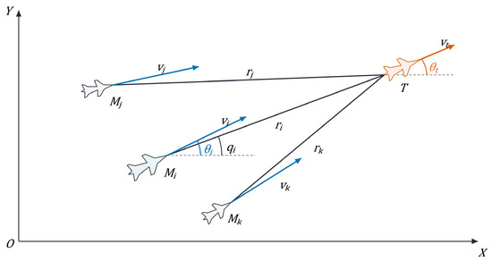
Figure 1 illustrates the multi-UAV engagement geometry. Fixed-wing UAVs M_j, M_i, and M_k approach the common maneuvering target T from different directions. Each solid segment connects a UAV nose to the target tail and represents the corresponding line of sight (LOS). The labels r_j, r_i, and r_k denote relative ranges, while v_j, v_i, and v_k denote vehicle speeds. The LOS angle q_i and heading angle θ_i are shown for the representative UAV M_i; the target speed and heading are v_T and θ_T. The communication graph is defined separately in Section 2.2.

Figure 1. Multi-UAV engagement geometry in the inertial frame.

2.2. Communication Graph and Cooperative Objectives

For a closing engagement with ${\dot{r}}_i<0$, the remaining flight time is approximated by

$$t_{\mathit{go},i}\approx -{\displaystyle \frac{r_i}{{\dot{r}}_i}}$$

(12)

Differentiating the approximation in Equation (12) gives

$${\dot{t}}_{\mathit{go},i}=-1+{\displaystyle \frac{r_i^2{\dot{q}}_i^2}{{\dot{r}}_i^2}}-{\displaystyle \frac{r_i{u}_{\mathit{ri}}}{{\dot{r}}_i^2}}+{\displaystyle \frac{w_{\mathit{ri}}{r}_i}{{\dot{r}}_i^2}}$$

(13)

and the predicted attack time is

$$t_{a,i}=t+t_{\mathit{go},i}=t-{\displaystyle \frac{r_i}{{\dot{r}}_i}}$$

(14)

For numerical evaluation, the estimated time-to-go $t_{\mathit{go},i}=-r_i/{\dot{r}}_i$ is recorded directly. Since the current time t is common to all vehicles,

t_a,i − t_a,j = t_go,i − t_go,j

(15)

so either variable produces the same graph-based consensus error. The theoretical development therefore uses t_a,i, while the numerical time-history figure reports t_go,i.

Differentiating t_a,i yields

$${\dot{t}}_{a,i}={\displaystyle \frac{r_i^2{\dot{q}}_i^2}{{\dot{r}}_i^2}}-{\displaystyle \frac{r_i}{{\dot{r}}_i^2}}{u}_{\mathit{ri}}+{\displaystyle \frac{r_i}{{\dot{r}}_i^2}}{w}_{\mathit{ri}}$$

(16)

Information exchange is represented by an undirected connected graph G = (V, E, A), where V = {1, …, N} is the node set, E is the edge set, and A = [a_ij] is the weighted adjacency matrix. The weight a_ij = a_ji > 0 if vehicles i and j exchange information and a_ij = 0 otherwise, with a_ii = 0. Let $D=\mathrm{diag}(\sum _j{a}_{1j},\dots ,\sum _j{a}_{\mathit{Nj}})$ and L = D − A. Because G is connected, the Laplacian satisfies 0 = λ₁(L) < λ₂(L)≤ ⋯ ≤λ_N(L). Hereafter, λ₂ = λ₂(L) denotes the algebraic connectivity. The predicted attack-time consensus error is defined as

$${\epsilon }_i={\displaystyle {\sum }_{j=1}^N}{a}_{\mathit{ij}}(t_{a,i}-t_{a,j})$$

(17)

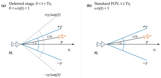
Two coupled objectives are imposed. First, the vehicles must reach consensus on their predicted attack times, equivalently on their remaining flight times, within the designer-selected time T. Second, the target must remain inside the transformed seeker FOV throughout the guidance interval and inside the standard FOV after the selected recovery time T_η. The cooperative objective is therefore to drive ε_i to zero within T, while the LOS-normal-direction channel satisfies the deferred FOV safety constraint. The LOS-direction and LOS-normal-direction designs are developed separately in the LOS frame and then coupled through the vehicle-frame command transformation and safety filter. Figure 2 illustrates the transition from the deferred stage to the recovered standard-FOV stage. When the target is outside the seeker FOV, r_i and q_i are supplied by external target indication such as a data link.

Figure 2. Deferred boundary establishment and recovery of the standard field of view: (a) deferred stage and (b) standard-FOV stage.

2.3. Prescribed-Time Preliminaries

Lemma 1

([30]). Consider the time-varying function μ_T(t) = T/(T − t). If a continuously differentiable positive function V: [0, T) → [0, +∞) satisfies

$$\dot{V}(t)\le -k{\mu }_T(t)V(t)+|d(t)|$$

(18)

where d(t) is an unknown perturbation satisfying $|d(t)|\le \overline{d}$ with $\overline{d}>0$, and k is a positive constant, then V(t) is bounded for t ∈ [0, T) and converges to zero as t → T.

Lemma 2.

Consider the nonlinear system $\dot{\mathit{x}}=f(\mathit{x},t)$. If there exists a continuously differentiable positive-definite Lyapunov function V(x) satisfying

$$\dot{V}(\mathit{x})\le -{\displaystyle \frac{1}{\beta T_c}}\mathit{exp}(V(\mathit{x}{)}^{\beta })V(\mathit{x}{)}^{1-\beta }+{\alpha }_0$$

(19)

where T_c > 0 and 0 < β ≤ 1, then, for α₀ = 0, the origin is strictly globally prescribed-time stable and its settling time does not exceed T_c for any initial condition.

Lemma 1 supplies the comparison argument used by time-varying prescribed-time gains, whereas Lemma 2 supplies the Lyapunov template used in the observer proofs. The proof of Lemma 1 is available in [30].

Proof of Lemma 2. 

Let t_s = inf{t ≥ 0: V(t) = 0}. If V(0) = 0, then t_s = 0. Otherwise, V(t) > 0 for 0 ≤ t < t_s. Define the strictly increasing function Φ(V) = 1 − exp(−V^β). Using (19) with α₀ = 0 gives, for 0 ≤ t < t_s,

$$\dot{\mathsf{\Phi }}(V)=\beta \exp (-V^{\beta })V^{\beta -1}\dot{V}\le -{\displaystyle \frac{1}{T_c}}.$$

Integrating over [0, t] yields Φ(V(t)) ≤ Φ(V(0)) − t/T_c. Since Φ(V(t)) ≥ 0 before the first hitting time, this inequality cannot hold beyond T_cΦ(V(0)). Therefore,

t_s ≤ T_cΦ(V(0)) = T_c[1 − exp(−V(0)^β)] < T_c

for every nonzero initial condition, while t_s = 0 at the origin. Positive definiteness and f(0, t) = 0 make the origin invariant thereafter. Hence, the system reaches and remains at the origin before T_c, proving prescribed-time convergence. □

3. Prescribed-Time Disturbance Observer Design

3.1. State Reconstruction and Assumption

To establish prescribed-time convergence of the disturbance estimates, first reconstruct the planar relative-motion model as two scalar second-order subsystems. This reconstruction preserves the radial/angular decomposition of Section 2.1 and identifies exactly which unknown term must be estimated in each channel. Define the state variables

$$x_{1i}=r_i,x_{2i}={\dot{r}}_i,x_{3i}=q_i,x_{4i}={\dot{q}}_i$$

(20)

The relative dynamics become

$${\dot{x}}_{1i}=x_{2i},{\dot{x}}_{2i}=x_{1i}{x}_{4i}^2-u_{\mathit{ri}}+d_{\mathit{ri}}$$

(21)

$${\dot{x}}_{3i}=x_{4i},{\dot{x}}_{4i}=-2x_{4i}{\displaystyle \frac{x_{2i}}{x_{1i}}}-{\displaystyle \frac{u_{\mathit{qi}}}{x_{1i}}}+d_{\mathit{qi}}$$

(22)

where d_ri = w_ri and d_qi = w_qi/r_i.

Assumption 1.

The target acceleration is continuously differentiable and has bounded variation. The lumped disturbances d_qi(t) and d_ri(t) are continuously differentiable and strictly bounded; that is, there exist known positive constants ${\overline{\mathsf{\Theta }}}_q$ and ${\overline{\mathsf{\Theta }}}_r$ such that $|d_{\mathit{qi}}(t)|\le {\overline{\mathsf{\Theta }}}_q$ and $|d_{\mathit{ri}}(t)|\le {\overline{\mathsf{\Theta }}}_r$ over the global time domain.

The known bounds in Assumption 1 are determined from the target’s maximum acceleration capability. The bounded-target-acceleration assumption is commonly adopted in guidance and disturbance-observer design [10,14,19,20,21].

The quantities treated as directly measured in the guidance model are the relative range, LOS angle, range rate, LOS angular rate, vehicle speed, and heading angle. The radial and angular lumped disturbances d_ri and d_qi are estimated by the prescribed-time observers, while only neighboring predicted attack times are exchanged through the communication graph.

3.2. Relative-Distance Disturbance Observer

For the radial state x_2i, define the observer state ${\widehat{x}}_{2i}$ and the aggregate-disturbance estimate ${\widehat{d}}_{\mathit{ri}}$. The prescribed-time observer is

$${\dot{\widehat{x}}}_{2i}=x_{1i}{x}_{4i}^2-u_{\mathit{ri}}+{\widehat{d}}_{\mathit{ri}}$$

(23)

$${\widehat{d}}_{\mathit{ri}}={\displaystyle \frac{1}{{\beta }_r{T}_c}}\exp \left(|e_{\mathit{ri}}{|}^{2{\beta }_r}\right)|e_{\mathit{ri}}{|}^{1-2{\beta }_r}\mathrm{sgn}(e_{\mathit{ri}})+{\mathsf{\Theta }}_r\mathrm{sgn}(e_{\mathit{ri}})$$

(24)

where $e_{\mathit{ri}}=x_{2i}-{\widehat{x}}_{2i}$ is the radial observation error, T_c > 0, 0 < β_r < 0.5, and ${\mathsf{\Theta }}_r>{\overline{\mathsf{\Theta }}}_r$.

Theorem 1.

For the relative-distance subsystem, under Assumption 1 and with the observer gain selected as ${\mathsf{\Theta }}_r>{\overline{\mathsf{\Theta }}}_r$, the observer guarantees that the relative-velocity observation error e_ri and the corresponding disturbance-estimation error $d_{\mathit{ri}}-{\widehat{d}}_{\mathit{ri}}$ converge globally to zero within the prescribed time T_c.

Proof. 

The radial observation-error dynamics are explicitly obtained as

$$\begin{array}{c}{\dot{e}}_{\mathit{ri}}={\dot{x}}_{2i}-{\dot{\widehat{x}}}_{2i}\\ =(x_{1i}{x}_{4i}^2-u_{\mathit{ri}}+d_{\mathit{ri}})-(x_{1i}{x}_{4i}^2-u_{\mathit{ri}}+{\widehat{d}}_{\mathit{ri}})\\ =d_{\mathit{ri}}(t)-{\widehat{d}}_{\mathit{ri}}\end{array}$$

(25)

Substituting the observer injection gives

$${\dot{e}}_{\mathit{ri}}=-{\displaystyle \frac{1}{{\beta }_r{T}_c}}\exp (|e_{\mathit{ri}}{|}^{2{\beta }_r})|e_{\mathit{ri}}{|}^{1-2{\beta }_r}\mathrm{sgn}(e_{\mathit{ri}})-{\mathsf{\Theta }}_r\mathrm{sgn}(e_{\mathit{ri}})+d_{\mathit{ri}}(t)$$

(26)

Define $V_{\mathit{ri}}=e_{\mathit{ri}}^2/2$. Its derivative is

$${\dot{V}}_{\mathit{ri}}=-{\displaystyle \frac{1}{{\beta }_r{T}_c}}\exp (|e_{\mathit{ri}}{|}^{2{\beta }_r})|e_{\mathit{ri}}{|}^{2-2{\beta }_r}-{\mathsf{\Theta }}_r|e_{\mathit{ri}}|+e_{\mathit{ri}}{d}_{\mathit{ri}}$$

(27)

Furthermore,

$$-{\mathsf{\Theta }}_r|e_{\mathit{ri}}|+e_{\mathit{ri}}{d}_{\mathit{ri}}\le -{\mathsf{\Theta }}_r|e_{\mathit{ri}}|+{\overline{\mathsf{\Theta }}}_r|e_{\mathit{ri}}|\le 0$$

(28)

because ${\mathsf{\Theta }}_r>{\overline{\mathsf{\Theta }}}_r$. Hence,

$${\dot{V}}_{\mathit{ri}}\le -{\displaystyle \frac{1}{{\beta }_r{T}_c}}\exp (|e_{\mathit{ri}}{|}^{2{\beta }_r})|e_{\mathit{ri}}{|}^{2-2{\beta }_r}$$

(29)

Using |e_ri| = (2V_ri)^1/2 yields

$${\dot{V}}_{\mathit{ri}}\le -{\displaystyle \frac{2^{1-{\beta }_r}}{{\beta }_r{T}_c}}\exp (2^{{\beta }_r}{V}_{\mathit{ri}}^{{\beta }_r})V_{\mathit{ri}}^{1-{\beta }_r}$$

(30)

Since 0 < β_r < 0.5, $2^{1-{\beta }_r}>1$ and $\exp (2^{{\beta }_r}{V}_{\mathit{ri}}^{{\beta }_r})>\exp (V_{\mathit{ri}}^{{\beta }_r})$. A conservative relaxation gives

$${\dot{V}}_{\mathit{ri}}\le -{\displaystyle \frac{1}{{\beta }_r{T}_c}}\exp (V_{\mathit{ri}}^{{\beta }_r})V_{\mathit{ri}}^{1-{\beta }_r}$$

(31)

By Lemma 2, V_ri and e_ri reach zero within T_c, yielding ${\widehat{d}}_{\mathit{ri}}\equiv d_{\mathit{ri}}$. □

Once e_ri = 0 is reached, invariance of the sliding set requires ${\dot{e}}_{\mathit{ri}}=d_{\mathit{ri}}-{\widehat{d}}_{\mathit{ri}}=0$ almost everywhere. Because ${\mathsf{\Theta }}_r>{\overline{\mathsf{\Theta }}}_r$, the robust injection can generate the equivalent value that balances the disturbance, and hence ${\widehat{d}}_{\mathit{ri}}=d_{\mathit{ri}}$ in the Filippov sense. Thus, the ideal sign-based observer reconstructs the disturbance exactly, whereas the smooth numerical implementation yields practical convergence.

The radial observer supplies the disturbance quantity required by the attack-time derivative without measuring the target acceleration components directly. Because d_ri = w_ri, the physical radial disturbance estimate is ${\widehat{w}}_{\mathit{ri}}={\widehat{d}}_{\mathit{ri}}$ and enters the LOS-direction guidance law.

3.3. LOS-Angle Disturbance Observer

Analogously, for the LOS angular-rate state x_4i, define the observer state ${\widehat{x}}_{4i}$ and the aggregate-disturbance estimate ${\widehat{d}}_{\mathit{qi}}$. The prescribed-time observer is

$${\dot{\widehat{x}}}_{4i}=-2x_{4i}{\displaystyle \frac{x_{2i}}{x_{1i}}}-{\displaystyle \frac{u_{\mathit{qi}}}{x_{1i}}}+{\widehat{d}}_{\mathit{qi}}$$

(32)

$${\widehat{d}}_{\mathit{qi}}={\displaystyle \frac{1}{{\beta }_q{T}_c}}\exp \left(|e_{\mathit{qi}}{|}^{2{\beta }_q}\right)|e_{\mathit{qi}}{|}^{1-2{\beta }_q}\mathrm{sgn}(e_{\mathit{qi}})+{\mathsf{\Theta }}_q\mathrm{sgn}(e_{\mathit{qi}})$$

(33)

where $e_{\mathit{qi}}=x_{4i}-{\widehat{x}}_{4i}$ is the angular observation error, T_c > 0, 0 < β_q < 0.5, and ${\mathsf{\Theta }}_q>{\overline{\mathsf{\Theta }}}_q$.

Theorem 2.

For the LOS-angle subsystem, under Assumption 1 and with the observer gain selected as ${\mathsf{\Theta }}_q>{\overline{\mathsf{\Theta }}}_q$, the observer guarantees that the observation error e_qi and the disturbance-estimation error $d_{\mathit{qi}}-{\widehat{d}}_{\mathit{qi}}$ converge globally to zero within the prescribed time T_c.

Proof. 

The angular observation-error dynamics are

$$\begin{array}{c}{\dot{e}}_{\mathit{qi}}={\dot{x}}_{4i}-{\dot{\widehat{x}}}_{4i}\\ =\left(-2x_{4i}{\displaystyle \frac{x_{2i}}{x_{1i}}}-{\displaystyle \frac{u_{\mathit{qi}}}{x_{1i}}}+d_{\mathit{qi}}\right)-\left(-2x_{4i}{\displaystyle \frac{x_{2i}}{x_{1i}}}-{\displaystyle \frac{u_{\mathit{qi}}}{x_{1i}}}+{\widehat{d}}_{\mathit{qi}}\right)\\ =d_{\mathit{qi}}(t)-{\widehat{d}}_{\mathit{qi}}\end{array}$$

(34)

Substitution of the observer injection gives

$${\dot{e}}_{\mathit{qi}}=-{\displaystyle \frac{1}{{\beta }_q{T}_c}}\exp (|e_{\mathit{qi}}{|}^{2{\beta }_q})|e_{\mathit{qi}}{|}^{1-2{\beta }_q}\mathrm{sgn}(e_{\mathit{qi}})+d_{\mathit{qi}}(t)-{\mathsf{\Theta }}_q\mathrm{sgn}(e_{\mathit{qi}})$$

(35)

Define $V_{\mathit{qi}}=e_{\mathit{qi}}^2/2$. Then

$${\dot{V}}_{\mathit{qi}}=-{\displaystyle \frac{1}{{\beta }_q{T}_c}}\exp (|e_{\mathit{qi}}{|}^{2{\beta }_q})|e_{\mathit{qi}}{|}^{2-2{\beta }_q}+e_{\mathit{qi}}{d}_{\mathit{qi}}(t)-{\mathsf{\Theta }}_q\mathrm{sgn}(e_{\mathit{qi}})e_{\mathit{qi}}$$

(36)

Under Assumption 1 and ${\mathsf{\Theta }}_q>{\overline{\mathsf{\Theta }}}_q$,

$$-{\mathsf{\Theta }}_q|e_{\mathit{qi}}|+e_{\mathit{qi}}{d}_{\mathit{qi}}\le -{\mathsf{\Theta }}_q|e_{\mathit{qi}}|+{\overline{\mathsf{\Theta }}}_q|e_{\mathit{qi}}|\le 0$$

(37)

Therefore,

$${\dot{V}}_{\mathit{qi}}\le -{\displaystyle \frac{2^{1-{\beta }_q}}{{\beta }_q{T}_c}}\exp (2^{{\beta }_q}{V}_{\mathit{qi}}^{{\beta }_q})V_{\mathit{qi}}^{1-{\beta }_q}$$

(38)

Since 0 < β_q < 0.5, a conservative relaxation gives

$${\dot{V}}_{\mathit{qi}}\le -{\displaystyle \frac{1}{{\beta }_q{T}_c}}\exp (V_{\mathit{qi}}^{{\beta }_q})V_{\mathit{qi}}^{1-{\beta }_q}$$

(39)

This differential inequality has the standard form of Lemma 2. Thus, V_qi and e_qi converge to zero within T_c, and the original disturbance d_qi(t) is reconstructed within the prescribed time. □

The angular observer is structurally parallel to the radial observer, but it estimates the range-normalized disturbance in the LOS-rate dynamics. After the observation error converges within T_c, the physical disturbance components required by the guidance laws are recovered as follows:

Using the variable mapping in Section 3.1 and x_1i = r_i, the observer outputs and the physical LOS-frame disturbances satisfy

$${\widehat{w}}_{\mathit{ri}}={\widehat{d}}_{\mathit{ri}},{\widehat{w}}_{\mathit{qi}}=r_i{\widehat{d}}_{\mathit{qi}}$$

(40)

The multiplication by r_i in the angular channel reverses the normalization d_qi = w_qi/r_i. The estimates developed in Section 3.2 and Section 3.3 can therefore be used directly by the two guidance channels in Section 4.

4. Cooperative Guidance Design and Analysis

4.1. LOS-Direction Attack-Time Consensus Guidance

With the target-maneuver terms reconstructed, the LOS-direction channel is designed to make the predicted attack times t_a,i reach consensus within the selected time T. Define ${\epsilon }_i={\displaystyle {\sum }_{j=1}^N}{a}_{\mathit{ij}}(t_{a,i}-t_{a,j})$. The first two terms of the following command cancel the known radial coupling and the reconstructed maneuver term, while the graph-dependent term drives the local attack-time disagreement. The LOS-direction guidance command is

$$u_{\mathit{ri}}=r_i{\dot{q}}_i^2+{\widehat{w}}_{\mathit{ri}}+{\displaystyle \frac{{\dot{r}}_i^2}{2{\lambda }_2{r}_i}}\varpi (t){\epsilon }_i$$

(41)

where λ₂ is the algebraic connectivity defined in Section 2.2, and

$$\varpi (t)=\left\{\begin{array}{ll}{\displaystyle \frac{a}{T-t}},& 0\le t<T,\\ a,& t\ge T,\end{array}\right.a>0$$

(42)

Theorem 3.

Under Assumption 1, if the communication graph is connected and 0 < T_c < T, the nominal LOS-direction guidance law drives the predicted attack-time consensus error to zero no later than T.

Proof. 

Let t_a = [t_a1, ⋯, t_aN]^T. To prove prescribed-time convergence of the consensus error, define

$$V_a={\mathbf{t}}_a^{T}L{\mathbf{t}}_a$$

(43)

Its time derivative is

$${\dot{V}}_a=2{\mathbf{t}}_a^{T}L{\dot{\mathbf{t}}}_a=2{\displaystyle {\sum }_{i=1}^N}{\displaystyle {\sum }_{j=1}^N}{a}_{\mathit{ij}}(t_{\mathit{ai}}-t_{\mathit{aj}})\left({\displaystyle \frac{r_i^2{\dot{q}}_i^2}{{\dot{r}}_i^2}}-{\displaystyle \frac{r_i{u}_{\mathit{ri}}}{{\dot{r}}_i^2}}+{\displaystyle \frac{w_{\mathit{ri}}{r}_i}{{\dot{r}}_i^2}}\right)$$

(44)

Substitution of the controller in Equation (41) gives

$${\dot{V}}_a=2{\displaystyle {\sum }_{i=1}^N}{\displaystyle {\sum }_{j=1}^N}{a}_{\mathit{ij}}(t_{\mathit{ai}}-t_{\mathit{aj}})\left(-{\displaystyle \frac{{\widehat{w}}_{\mathit{ri}}{r}_i}{{\dot{r}}_i^2}}-{\displaystyle \frac{1}{2{\lambda }_2}}\varpi {\epsilon }_i+{\displaystyle \frac{w_{\mathit{ri}}{r}_i}{{\dot{r}}_i^2}}\right)$$

(45)

The design uses 0 < T_c < T so that exact disturbance reconstruction is established before the consensus deadline. For T_c < t < T, it follows that

$${\dot{V}}_a=-2{\displaystyle {\sum }_{i=1}^N}{\displaystyle {\sum }_{j=1}^N}{a}_{\mathit{ij}}(t_{\mathit{ai}}-t_{\mathit{aj}}){\displaystyle \frac{1}{2{\lambda }_2}}{\displaystyle \frac{a}{T-t}}{\epsilon }_i$$

(46)

Therefore,

$${\dot{V}}_a\le -{\displaystyle \frac{1}{{\lambda }_2}}{\displaystyle \frac{a}{T-t}}{\displaystyle {\sum }_{i=1}^N}{\epsilon }_i^2$$

(47)

Noting that

$${\displaystyle {\sum }_{i=1}^N}{\epsilon }_i^2={\left(L^{{\displaystyle \frac{1}{2}}}{\mathbf{t}}_a\right)}^{T}L\left(L^{{\displaystyle \frac{1}{2}}}{\mathbf{t}}_a\right)\ge {\lambda }_2{\mathbf{t}}_a^{T}L{\mathbf{t}}_a={\lambda }_2{V}_a$$

(48)

one obtains

$${\dot{V}}_a\le -{\displaystyle \frac{a}{T-t}}{V}_a$$

(49)

Direct integration from T_c gives

$$V_a(t)\le V_a(T_c){\left({\displaystyle \frac{T-t}{T-T_c}}\right)}^a,T_c\le t<T$$

(50)

so V_a and the nominal consensus error approach zero as t → T⁻. For the nominal subsystem and t ≥ T,

$$\begin{array}{c}{\dot{V}}_a=2{\displaystyle {\sum }_{i=1}^N}{\epsilon }_i\left(-{\displaystyle \frac{{\widehat{w}}_{\mathit{ri}}{r}_i}{{\dot{r}}_i^2}}-{\displaystyle \frac{1}{2{\lambda }_2}}a{\epsilon }_i+{\displaystyle \frac{w_{\mathit{ri}}{r}_i}{{\dot{r}}_i^2}}\right)\\ \le -{\displaystyle \frac{1}{{\lambda }_2}}a{\displaystyle {\sum }_{i=1}^N}{\epsilon }_i^2\end{array}$$

(51)

It follows further that

$${\dot{V}}_a\le -a{V}_a$$

(52)

Since V_a(T) = 0, V_a(t) = 0, ∀t ≥ T. □

The proof follows the physical sequence of the design: disturbance compensation reduces the predicted-attack-time dynamics to a graph-consensus channel, algebraic connectivity converts the local disagreements into a bound on V_a, and the singular gain fixes the convergence deadline. This sequence also explains why T_c < T is required: exact reconstruction must be available before the LOS-direction attack-time consensus surface is reached.

4.2. LOS-Normal-Direction Prescribed-Time Guidance

For effective interception, the LOS-normal-direction channel must drive ${\dot{q}}_i$ to zero. At the same time, the target should remain inside the seeker FOV during the terminal phase. The nominal controller is first constructed without the safety correction so that its LOS-rate convergence mechanism can be stated explicitly. The prescribed-time LOS-rate command is

$$u_{\mathit{qi}}^{\mathrm{nom}}=-2{\dot{r}}_i{\dot{q}}_i+r_i{\varpi }_q(t){\dot{q}}_i+{\widehat{w}}_{\mathit{qi}}$$

(53)

where

$${\varpi }_q(t)=\left\{\begin{array}{ll}{\displaystyle \frac{a_q}{T_q-t}},& 0\le t<T_q,\\ a_q,& t\ge T_q,\end{array}\right.a_q>0$$

(54)

Theorem 4.

Under Assumption 1, 0 < T_c < T_q, and angular-disturbance reconstruction for t ≥ T_c, the nominal LOS-normal-direction guidance law drives ${\dot{q}}_i$ to zero no later than T_q.

Proof. 

Define the Lyapunov function

$$V_{q,i}={\dot{q}}_i^2$$

(55)

Its derivative is

$${\dot{V}}_{q,i}=2{\dot{q}}_i{\ddot{q}}_i=2{\dot{q}}_i\left(-{\displaystyle \frac{2{\dot{r}}_i{\dot{q}}_i}{r_i}}-{\displaystyle \frac{u_{\mathit{qi}}}{r_i}}+{\displaystyle \frac{w_{\mathit{qi}}}{r_i}}\right)$$

(56)

Substitution of the prescribed-time controller in Equation (53) gives

$${\dot{V}}_{q,i}=2{\dot{q}}_i\left(-{\displaystyle \frac{2{\dot{r}}_i{\dot{q}}_i}{r_i}}+{\displaystyle \frac{2{\dot{r}}_i{\dot{q}}_i}{r_i}}-{\varpi }_q{\dot{q}}_i-{\displaystyle \frac{{\widehat{w}}_{\mathit{qi}}}{r_i}}+{\displaystyle \frac{w_{\mathit{qi}}}{r_i}}\right)=-2{\varpi }_q{\dot{q}}_i^2$$

(57)

For T_c ≤ t < T_q,

$${\dot{V}}_{q,i}=-{\displaystyle \frac{2a_q}{T_q-t}}{V}_{q,i}$$

(58)

Integration from T_c gives

$$V_{q,i}(t)=V_{q,i}(T_c){\left({\displaystyle \frac{T_q-t}{T_q-T_c}}\right)}^{2a_q},T_c\le t<T_q$$

(59)

and therefore V_q,i approaches zero as $t\to T_q^{-}$. For the nominal subsystem and t ≥ T_q,

$${\dot{V}}_{q,i}\le -2a_q{V}_{q,i}$$

(60)

Because ${\lim }_{t\to T_q}{V}_{q,i}=0$, it follows that V_q,i(t) = 0, ∀t ≥ T_q, and hence ${\dot{q}}_i=0,\forall t\ge T_q$ for the nominal pre-filter subsystem. □

After angular-disturbance reconstruction, cancellation of the known kinematic coupling and target-maneuver term reduces the ideal LOS-normal channel to scalar prescribed-time LOS-rate dynamics. This nominal command becomes the performance input to the deferred-FOV CBF-QP safety layer developed in Section 4.3 and Section 4.4.

4.3. Deferred FOV Constraint

To maintain effective tracking and interception while the LOS rate is regulated, introduce the velocity lead angle and a deferred FOV constraint. Define the velocity lead angle as

γ_i = q_i − θ_i

(61)

The standard field-of-view constraint is defined by the constant seeker limit

$$|{\gamma }_i|<\overline{\gamma }$$

(62)

To avoid overly strict early-stage constraints, introduce the time transformation

$${\varpi }_{\eta }=\left\{\begin{array}{ll}1-\exp \left({\displaystyle \frac{-a{t}^2}{T_{\eta }-t}}\right),& t<T_{\eta },\\ 1,& t\ge T_{\eta }\end{array}\right.$$

(63)

and impose the deferred field-of-view constraint

$${\varpi }_{\eta }|{\gamma }_i|<\overline{\gamma }$$

(64)

At t = 0, ϖ_η = 0, so the final seeker boundary is inactive during the initial geometry-adjustment instant. For 0 < t < T_η, ϖ_η(t) increases smoothly and establishes the FOV boundary; for t ≥ T_η, ϖ_η(t) = 1, and the standard FOV constraint is recovered. In both panels of Figure 2, the horizontal black ray is the vehicle velocity direction v_i, the slanted black segment is the LOS from the UAV nose to the target tail, and γ_i is the angle from v_i to the LOS. Figure 2a shows the deferred bounds ±γ/ϖ_η(t) together with the standard bounds ±γ for 0 < t < T_η, whereas Figure 2b shows the standard FOV after ϖ_η(t) = 1.

In (62)–(64), γ denotes the allowable upper bound of |γ_i|, T_η is the prescribed FOV-recovery time, a > 0 is the rate parameter governing the transition of ϖ_η(t), and ϖ_η(t) is the dimensionless transformation factor that increases from zero to one.

Using

$$x_{4i}={\dot{q}}_i=-{\displaystyle \frac{v_T\sin (q_i-{\theta }_T)}{r_i}}+{\displaystyle \frac{v_i\sin ({\gamma }_i)}{r_i}}$$

(65)

the deferred FOV construction is associated with the following transformed LOS-rate interval

λ_1,i ≤ ϖ_ηx_4i ≤ λ_2,i

(66)

where

$${\lambda }_{1,i}=-{\displaystyle \frac{v_T\sin (q_i-{\theta }_T)}{r_i}}-{\displaystyle \frac{v_i\sin (\overline{\gamma })}{r_i}}$$

(67)

$${\lambda }_{2,i}=-{\displaystyle \frac{v_T\sin (q_i-{\theta }_T)}{r_i}}+{\displaystyle \frac{v_i\sin (\overline{\gamma })}{r_i}}$$

(68)

Since 0 < γ < π/2 and v_i/r_i > 0 during the engagement, it follows that λ_1,i < λ_2,i; therefore, the transformed LOS-rate interval is nonempty.

The original deferred FOV requirement is subsequently enforced directly through the barrier functions introduced in Section 4.4.

4.4. CBF-QP Safety Filter

To enforce the deferred FOV constraint, introduce two control barrier functions, one for each side of the symmetric seeker aperture:

$$h_{\gamma ,1,i}={\varpi }_{\eta }{\gamma }_i+\overline{\gamma }\ge 0$$

(69)

$$h_{\gamma ,2,i}=-{\varpi }_{\eta }{\gamma }_i+\overline{\gamma }\ge 0$$

(70)

For positive CBF gains ϑ_1,i and ϑ_2,i, sufficient forward-invariance conditions for the FOV safe set can be written as [36]

$${\dot{h}}_{\gamma ,1,i}\ge -{\vartheta }_{1,i}{h}_{\gamma ,1,i}$$

(71)

$${\dot{h}}_{\gamma ,2,i}\ge -{\vartheta }_{2,i}{h}_{\gamma ,2,i}$$

(72)

Using the relative-motion equations gives

$$\begin{array}{c}{\dot{h}}_{\gamma ,1,i}={\varpi }_{\eta }({\dot{q}}_i-{\dot{\theta }}_i)+{\dot{\varpi }}_{\eta }(q_i-{\theta }_i)\\ ={\varpi }_{\eta }\left({\displaystyle \frac{v_T\sin ({\theta }_T-q_i)-v_i\sin ({\theta }_i-q_i)}{r_i}}-{\displaystyle \frac{a_{\mathit{hi}}}{v_i}}\right)+{\dot{\varpi }}_{\eta }(q_i-{\theta }_i)\ge -{\vartheta }_{1,i}{h}_{\gamma ,1,i}\end{array}$$

(73)

and

$$\begin{array}{c}{\dot{h}}_{\gamma ,2,i}={\varpi }_{\eta }(-{\dot{q}}_i+{\dot{\theta }}_i)+{\dot{\varpi }}_{\eta }(-q_i+{\theta }_i)\\ ={\varpi }_{\eta }\left(-{\displaystyle \frac{v_T\sin ({\theta }_T-q_i)-v_i\sin ({\theta }_i-q_i)}{r_i}}+{\displaystyle \frac{a_{\mathit{hi}}}{v_i}}\right)+{\dot{\varpi }}_{\eta }(-q_i+{\theta }_i)\ge -{\vartheta }_{2,i}{h}_{\gamma ,2,i}\end{array}$$

(74)

Here,

$${\dot{\varpi }}_{\eta }=\left\{\begin{array}{ll}{\displaystyle \frac{\mathit{at}(2T_{\eta }-t)}{(T_{\eta }-t{)}^2}}\exp \left({\displaystyle \frac{-a{t}^2}{T_{\eta }-t}}\right),& t<T_{\eta },\\ 0,& t\ge T_{\eta }\end{array}\right.$$

(75)

Let ${\overline{a}}_{\mathit{hi}}$ denote the nominal normal acceleration obtained by transforming the LOS-direction and nominal LOS-normal-direction commands into the vehicle frame. The corrected command $a_{\mathit{hi}}^{\star }$ is the solution of the scalar CBF-QP

$$\begin{array}{c}{a}_{\mathit{hi}}^{\star }=\underset{a_{\mathit{hi}}\in \mathbb{R}}{\mathrm{argmin}}{\left|a_{\mathit{hi}}-{\overline{a}}_{\mathit{hi}}\right|}^2\\ \mathrm{subject} \mathrm{to} {\varpi }_{\eta }\left(-{\displaystyle \frac{v_T\sin ({\theta }_T-q_i)-v_i\sin ({\theta }_i-q_i)}{r_i}}+{\displaystyle \frac{a_{\mathit{hi}}}{v_i}}\right)+{\dot{\varpi }}_{\eta }(-q_i+{\theta }_i)\ge -{\vartheta }_{2,i}{h}_{\gamma ,2,i},\\ {\varpi }_{\eta }\left({\displaystyle \frac{v_T\sin ({\theta }_T-q_i)-v_i\sin ({\theta }_i-q_i)}{r_i}}-{\displaystyle \frac{a_{\mathit{hi}}}{v_i}}\right)+{\dot{\varpi }}_{\eta }(q_i-{\theta }_i)\ge -{\vartheta }_{1,i}{h}_{\gamma ,1,i}\\ -a_{h,\max }\le a_{\mathit{hi}}\le a_{h,\max }\end{array}$$

(76)

For t > 0, ϖ_η > 0, and the two constraints are equivalent to the interval

$${\underset{\_}{a}}_{\mathit{hi}}={\displaystyle \frac{v_i}{{\varpi }_{\eta }}}\left({\varpi }_{\eta }{\dot{q}}_i+{\dot{\varpi }}_{\eta }{\gamma }_i-{\vartheta }_{2,i}{h}_{\gamma ,2,i}\right)\le a_{\mathit{hi}}\le {\displaystyle \frac{v_i}{{\varpi }_{\eta }}}\left({\varpi }_{\eta }{\dot{q}}_i+{\dot{\varpi }}_{\eta }{\gamma }_i+{\vartheta }_{1,i}{h}_{\gamma ,1,i}\right)={\overline{a}}_{\mathit{hi}}$$

(77)

With the input-amplitude constraint, the bounded feasible interval used by the QP is ${\mathcal{I}}_i(t)=[{\underset{\_}{a}}_{\mathit{hi}},{\overline{a}}_{\mathit{hi}}]\cap [-a_{h,\max },a_{h,\max }]$.

On the safe set,

$${\overline{a}}_{\mathit{hi}}-{\underset{\_}{a}}_{\mathit{hi}}={\displaystyle \frac{v_i}{{\varpi }_{\eta }}}\left({\vartheta }_{1,i}{h}_{\gamma ,1,i}+{\vartheta }_{2,i}{h}_{\gamma ,2,i}\right)\ge 0$$

(78)

At t = 0, ${\varpi }_{\eta }={\dot{\varpi }}_{\eta }=0$ and h_γ,1,i = h_γ,2,i = γ, so both CBF inequalities are automatically satisfied. With the acceleration bound in (76), the feasible set of the QP is the intersection of the CBF-admissible interval and the actuator interval [−a_h,max, a_h,max]. When this intersection is nonempty, the QP selects the feasible acceleration closest to the nominal command, and the resulting $a_{\mathit{hi}}^{\star }$ is applied to the vehicle.

Proposition 1.

For t > 0, suppose the transformed state is safe and the nominal normal acceleration satisfies ${\overline{a}}_{\mathit{hi}}\in {\mathcal{I}}_i(t)$. Then the unique solution of (76) is $a_{\mathit{hi}}^{\star }={\overline{a}}_{\mathit{hi}}$. Thus, the CBF-QP leaves the nominal prescribed-time command unchanged whenever that command satisfies the FOV-related CBF inequalities and the acceleration bound.

Proof. 

The scalar QP projects ${\overline{a}}_{\mathit{hi}}$ onto $ℐ$_i(t). If ${\overline{a}}_{\mathit{hi}}$ is feasible, the unique minimum is zero at $a_{\mathit{hi}}^{\star }={\overline{a}}_{\mathit{hi}}$; hence, the vehicle- and LOS-frame commands are unchanged, and Theorems 3 and 4 are retained. Otherwise, the projection enforces the CBF condition; Section 5 evaluates the resulting closed loop. Thus, under the stated feasibility condition, the nominal prescribed-time convergence guarantees are preserved. □

The prescribed consensus and FOV-recovery times are therefore selected so that the safety correction is completed within the prescribed interval.

Remark 1

(limitations and real-time implementation). The main limitations of the present study are its two-dimensional engagement model and ideal-communication assumption. Consequently, the theoretical guarantees established here do not directly extend to three-dimensional engagement geometry or networks subject to communication delays and packet loss. Addressing these effects requires corresponding extensions of the relative-motion model and convergence analysis. The nominal controller is analytical, and the CBF safety filter is the scalar QP in (76), so the resulting online computation remains suitable for real-time implementation.

5. Simulation Results

5.1. Simulation Setup and Numerical Implementation

The simulations are conducted in MATLAB/Simulink R2025b for the high-level guidance layer of three fixed-wing UAVs and one maneuvering aerial target in a two-dimensional plane. Each simulated UAV has local relative-state information and exchanges the predicted attack-time variable only with its graph neighbors. Ideal communication and ideal tracking of the commanded normal and tangential accelerations are assumed; no six-degree-of-freedom airframe or autopilot dynamics are included. The communication topology is the three-vehicle chain

$$A=\left[\begin{array}{ccc}0& 1& 0\\ 1& 0& 1\\ 0& 1& 0\end{array}\right]$$

(79)

The chain topology is undirected and connected, satisfying the graph condition in Theorem 3. Vehicles 1 and 3 exchange information through vehicle 2. Their distinct initial positions, speeds, and headings produce different ranges and remaining flight times, thereby activating both timing coordination and LOS-normal regulation.

The initial conditions are listed in Table 1.

Table 1. Initial conditions.

Object	Initial Position (x0, y0) (m)	Speed (m/s)	Heading Angle (Rad)
M1	(1000, 3000)	160	0.2
M2	(1200, 2000)	170	0.2
M3	(1500, 1000)	165	0.3
Target	(4000, 1500)	50	0.0

Table 2 lists the main controller parameters used in the numerical simulation.

Table 2. Main controller parameters used in the numerical simulation.

Category	Parameter	Value	Description
Attack-time consensus	T	5 s	Prescribed consensus time
Attack-time consensus	a	2	Dimensionless gain in ϖ = a/(T − t)
Disturbance observer	Tc	4 s	Prescribed observer convergence time
Disturbance observer	βr, βq	0.1, 0.1	Dimensionless observer exponent parameters
Disturbance observer	Θr, Θq	0.1, 50.6	Observer robust gains (model-consistent units)
LOS-normal-direction control	Tq	5 s	Prescribed LOS-rate convergence time
LOS-normal-direction control	aq	2	Dimensionless gain in ϖq = aq/(Tq − t)
Deferred FOV	Tη	2 s	Delay time for restoring the standard FOV boundary
Deferred FOV	$\overline{\gamma }$	0.4 rad	Final field-of-view boundary
CBF-QP	ϑ1, ϑ2	10, 10 s−1	CBF gains used in the implementation

The maneuvering target uses constant tangential and normal accelerations

a_zT = 0.1 m/s², a_hT = 0.1 m/s²

(80)

Although the target accelerations are constant, their projections onto the vehicle-dependent LOS frames vary with the engagement geometry. The observer inputs d_ri and d_qi are therefore time-varying.

The simulations use the variable-step, variable-order ode15s solver for stiff differential equations over 0 ≤ t ≤ 29.56 s, with a maximum step size of 0.1 s, a relative tolerance of 10⁻⁵, and automatic absolute-tolerance scaling. The scalar QP is solved by quadprog with the active-set algorithm and a maximum of 100 iterations.

The radial and angular disturbance observers use Θ_rsgn(e_ri) and Θ_qsgn(e_qi), respectively, in the theoretical analysis. To suppress high-frequency switching in the numerical simulation, Simulink implements the two robust terms as

$${\mathsf{\Theta }}_r\tanh \left({\displaystyle \frac{e_{\mathit{ri}}}{0.1}}\right),{\displaystyle \frac{{\mathsf{\Theta }}_q}{r_i}}\tanh \left({\displaystyle \frac{e_{\mathit{qi}}}{0.01}}\right)$$

(81)

The simulations replace the observer sign functions with hyperbolic-tangent boundary layers; the resulting observer errors therefore exhibit practical rather than exact convergence.

For quantitative reporting, the consensus settling time is the earliest recorded instant after which max_i|ε_i| ≤ 10⁻² holds for the remainder of the simulation. The deferred-FOV margin is $\overline{\gamma }-{\max }_i|{\varpi }_{\eta }{\gamma }_i|$, whereas the post-delay standard-FOV margin is $\overline{\gamma }-{\max }_i|{\gamma }_i|$ for t ≥ T_η. The 10⁻² threshold is used to report sampled simulation signals, whereas the analytical convergence results refer to the ideal nominal model.

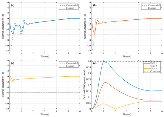
For the finite-actuation case, in (76), a ±6 g bound followed by a first-order acceleration response was used with a 0.1 s time constant. The corresponding acceleration-loop response is reported in Section 5.2. The 2% settling time is about 0.4 s. The minimum deferred-FOV margin is 0.001816 rad, the peak realized acceleration is 5.665 g, and the final maximum attack-time consensus error is 1.181 × 10⁻⁸ s.

5.2. Coordination, Observation, FOV, and Control Responses

Figure 3, Figure 4, Figure 5, Figure 6, Figure 7 and Figure 8 report the attack-time coordination, observer errors, FOV response, command histories, planar engagement trajectories, and acceleration-loop response.

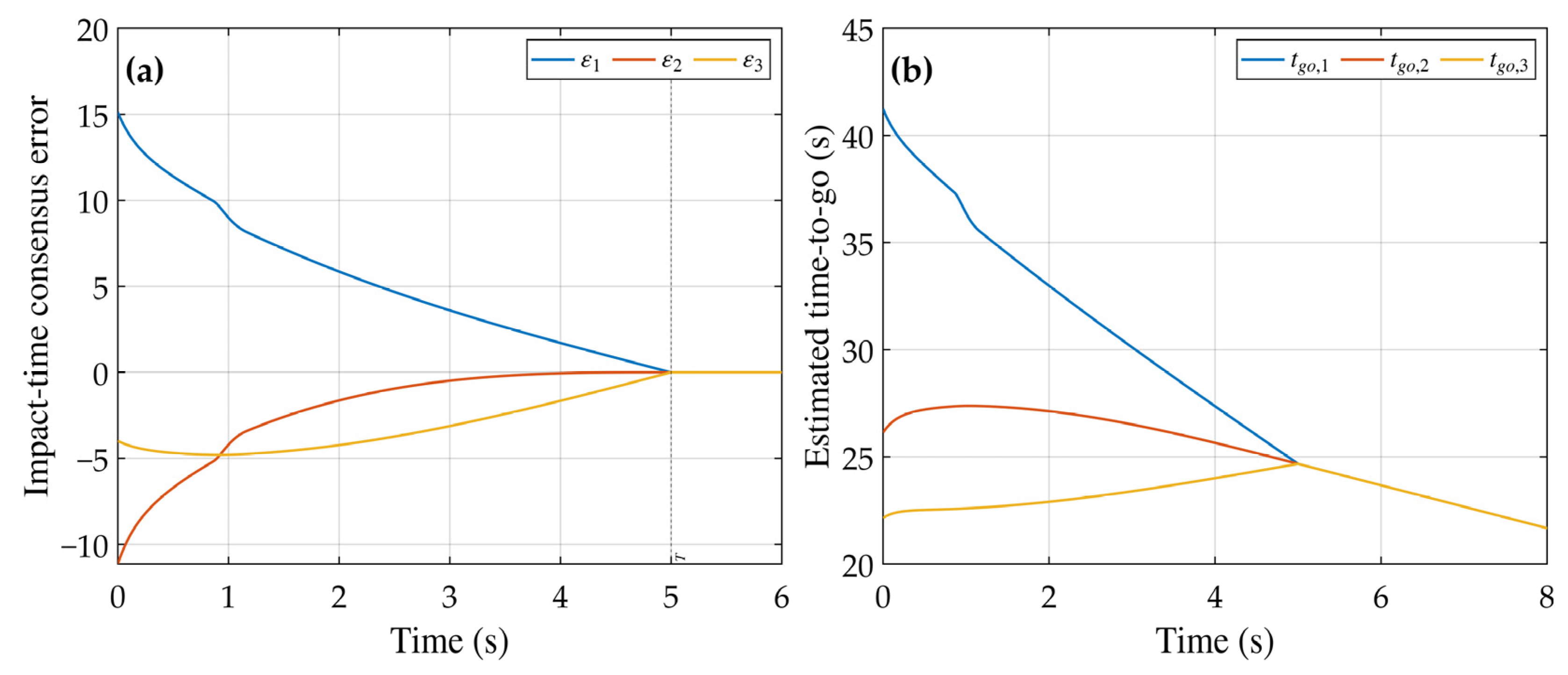
Figure 3. Attack-time coordination: (a) attack-time consensus errors and (b) estimated time-to-go trajectories.

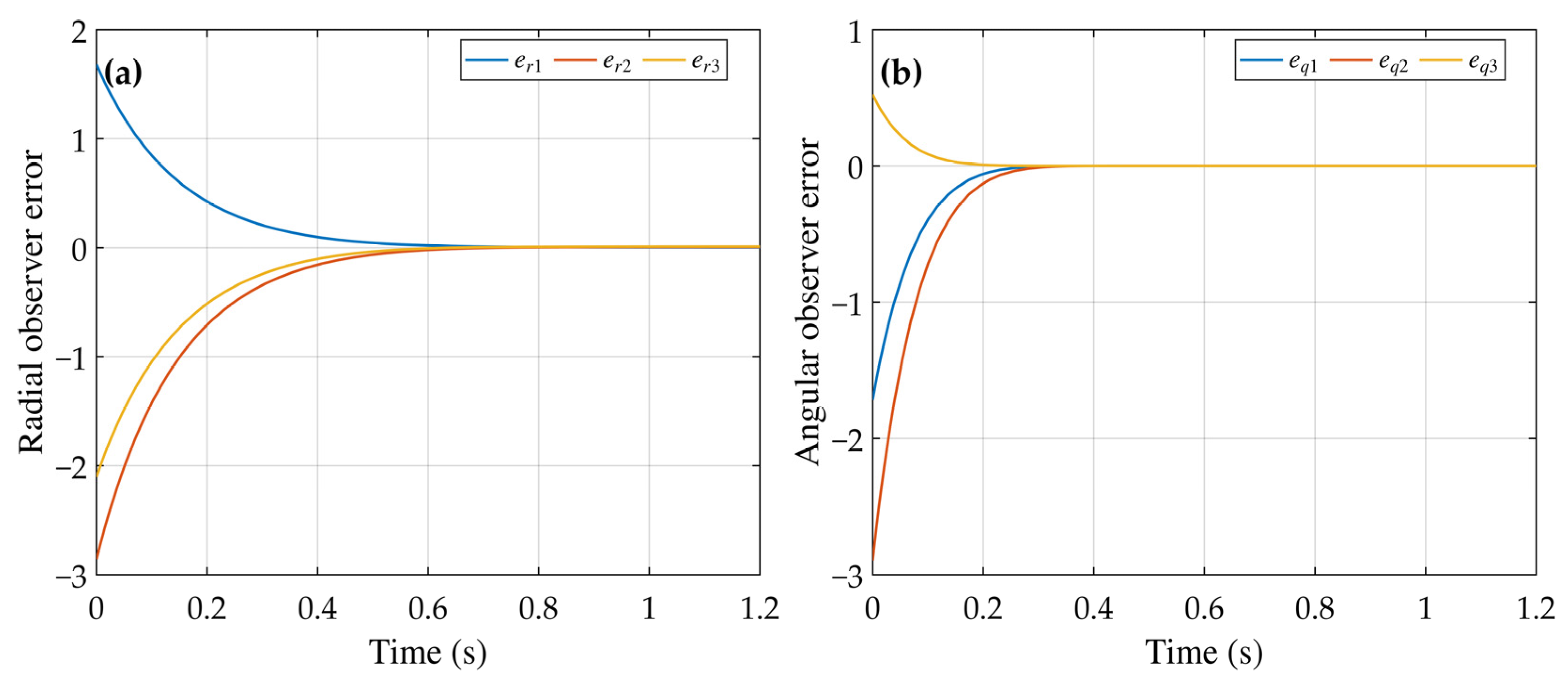
Figure 4. Disturbance-observer errors: (a) radial observer errors and (b) angular observer errors.

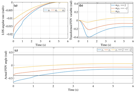
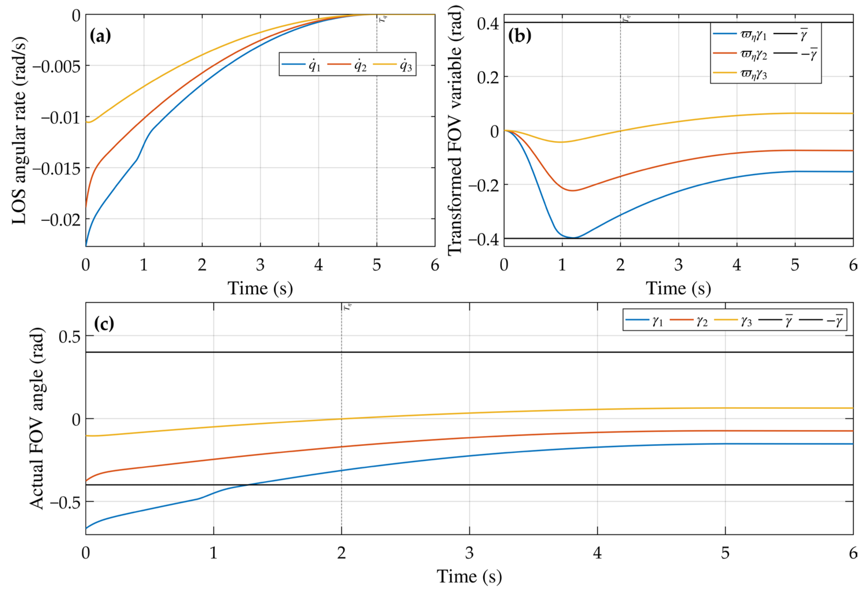
Figure 5. LOS-rate and deferred-FOV responses: (a) LOS angular rates, (b) transformed velocity lead angles and FOV bounds, and (c) actual velocity lead angles and standard FOV bounds.

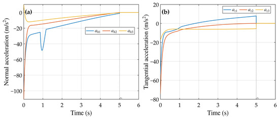
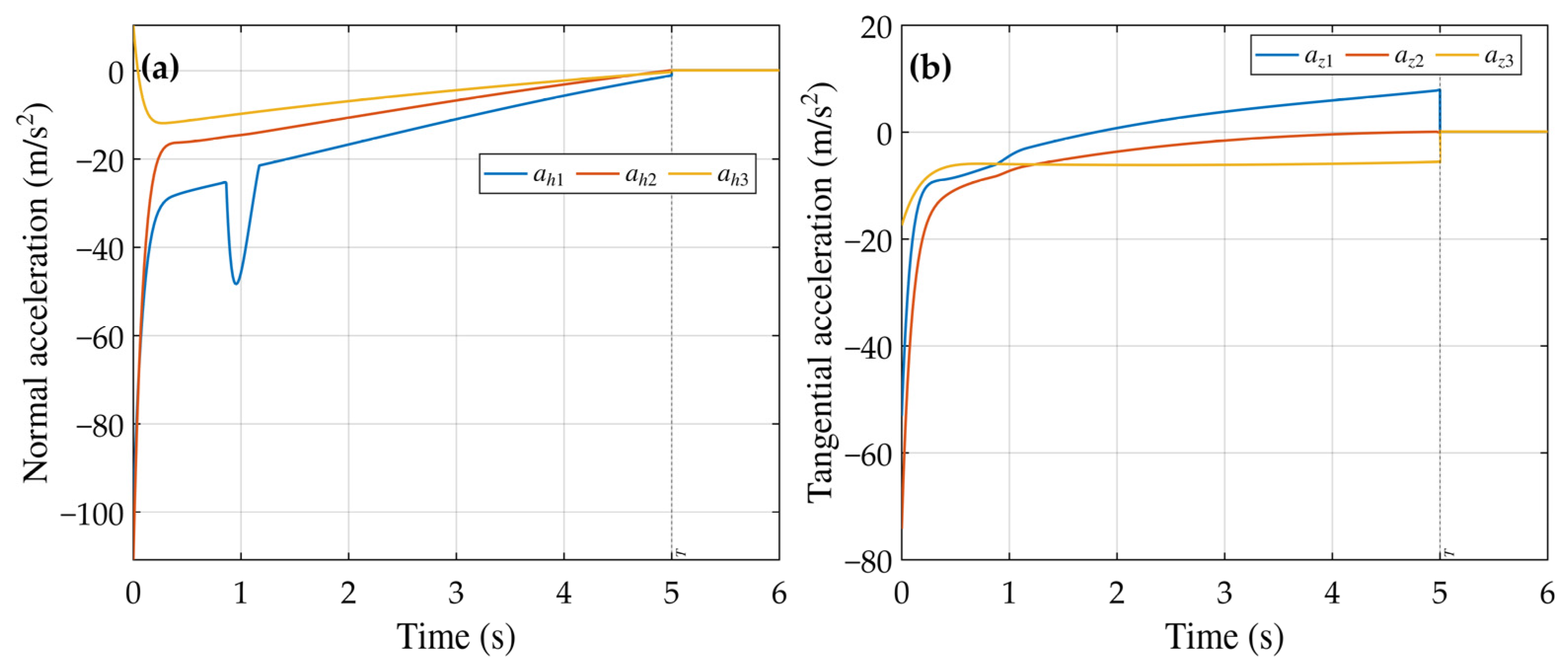
Figure 6. Vehicle-frame guidance commands: (a) normal accelerations and (b) tangential accelerations.

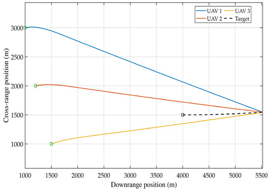
Figure 7. Planar interception trajectories. Green circles and the black square indicate the initial positions of the UAVs and the target, respectively.

Figure 8. Acceleration-loop response: (a–c) commanded and realized normal accelerations of UAVs 1–3 and (d) deferred-FOV quantities and constraint.

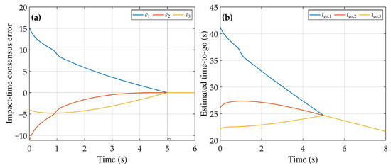
Figure 3 presents attack-time coordination. Figure 3a shows the consensus-error transient over 0–6 s, with the dashed line marking T = 5 s. At the 10⁻² reporting threshold, the measured settling time is 4.998 s, and the final maximum absolute consensus error is 1.05 × 10⁻⁸. Figure 3b shows the estimated time-to-go trajectories over 0–8 s; they approach a common value with a final spread of 6.41 × 10⁻⁹ s. Because pairwise differences in t_a,i and t_go,i are identical, these histories also support predicted attack-time consensus.

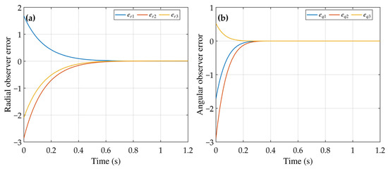
Figure 4 shows the disturbance-observer transients over 0–1.2 s: Figure 4a gives the radial errors and Figure 4b the angular errors; the prescribed value T_c = 4 s lies outside this zoomed interval. The final maximum angular-channel error is 2.56 × 10⁻⁵. The radial-channel error decreases substantially and remains bounded, with a final maximum magnitude of 1.09 × 10⁻².

Figure 5 focuses on the 0–6 s interval. Figure 5a gives the LOS angular rates with T_q = 5 s marked by the dashed line, while Figure 5b gives the transformed lead angles ϖ_ηγ_i and bounds ±γ with T_η = 2 s marked. The complete trajectory yields a minimum deferred-FOV margin of 0.00194 rad, a minimum post-delay standard-FOV margin of 0.0948 rad, and a maximum absolute LOS angular rate of 0.0227 rad/s. Figure 5c reports the actual velocity lead angles. Their maximum absolute value is 0.6636 rad during the deferred stage; this early excursion is permitted by the relaxed boundary, while all three trajectories remain within the standard 0.4 rad limit after the 2 s recovery time.

Figure 6 gives the vehicle-frame commands over 0–6 s. Figure 6a shows the normal accelerations and Figure 6b the tangential accelerations, with the dashed line marking T = 5 s. Their maximum absolute values are 110.78 m/s² and 74.21 m/s², respectively.

Figure 7 shows the complete planar trajectories of the three vehicles and the maneuvering target, illustrating how the vehicles approach the common target region from different initial positions.

Figure 8 shows that the first-order response keeps the realized normal accelerations within 6 g and the deferred-FOV quantities below 0.4 rad.

5.3. Quantitative Summary

Table 3 summarizes the numerical indicators reported with Figure 3, Figure 4, Figure 5, Figure 6 and Figure 7.

Table 3. Quantitative results for the three-UAV numerical case.

Quantity	Reported Value	Interpretation
Consensus settling time at 10−2 s threshold	4.998 s	Within selected T = 5 s
Final maximum consensus error	1.05 × 10−8 s	Numerical agreement
Final time-to-go spread	6.41 × 10−9 s	Numerical agreement
Final maximum angular observer error	2.56 × 10−5 rad/s	Below reporting threshold
Final maximum radial observer error	1.09 × 10−2 m/s	Practical attenuation
Minimum deferred-FOV margin	0.00194 rad	Positive over full simulation
Minimum standard-FOV margin after Tη	0.0948 rad	Positive after boundary recovery
Maximum absolute LOS angular rate	0.0227 rad/s	Bounded in evaluated case
Maximum |ahi|/|azi|	110.78/74.21 m/s2	Simulated control demand

Table 3 shows that the attack-time disagreement crosses the selected threshold before T, both FOV margins remain positive, and both observer errors decrease. The radial error remains slightly above the selected threshold, while the acceleration extrema quantify the simulated control demand.

5.4. CBF-QP Ablation and Validation Under Nonideal Conditions

Table 4 isolates the CBF-QP effect under otherwise identical settings. Removing the projection raises the maximum deferred-FOV quantity to 0.425610 rad and causes a 0.475 s violation; the complete method remains below 0.4 rad.

Table 4. CBF-QP ablation under identical baseline conditions.

Case	Maximum Deferred-FOV Quantity (Rad)	Violation Duration (s)	Minimum Deferred-FOV Margin (Rad)	Largest Vehicle-Wise Minimum Miss Distance (m)
Complete method	0.398119	0	0.001881	13.279971
Without CBF-QP	0.425610	0.475	−0.025610	44.521892

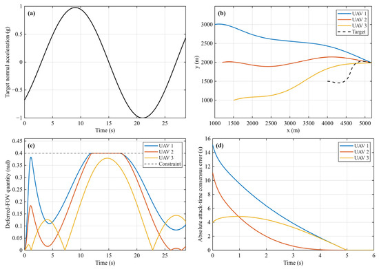
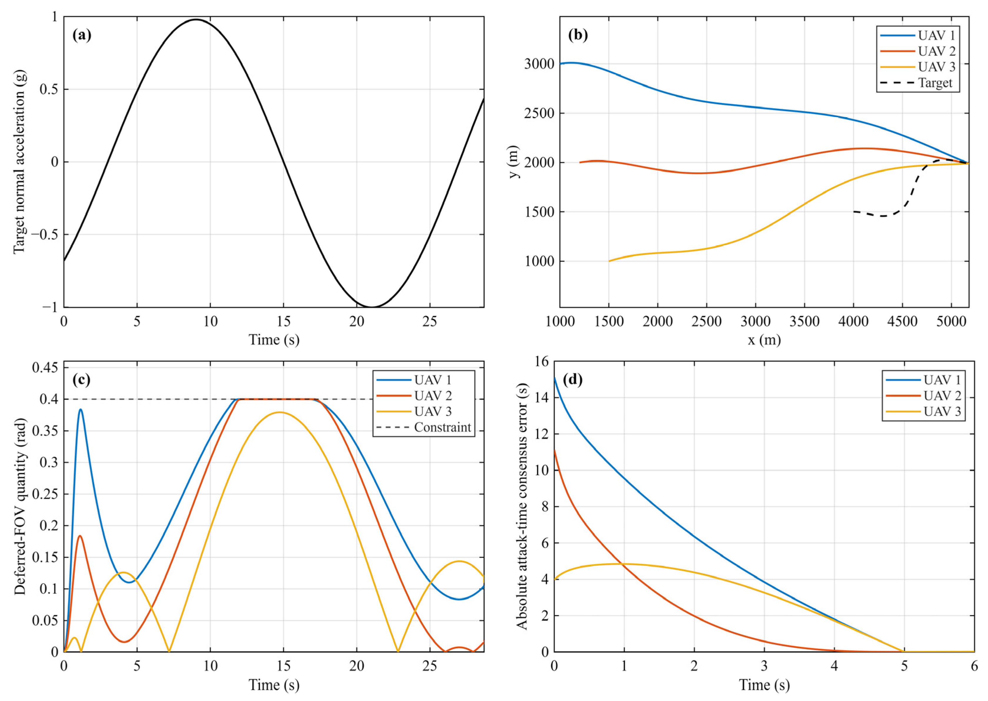
Figure 9 evaluates the sinusoidal target normal acceleration a_T,n(t) = 9.42947sin(πt/12 − π/4) m/s². No deferred-FOV violation is detected at the 10⁻⁹ rad numerical tolerance. The three minimum miss distances are 0.01036, 0.01148, and 0.02371 m, and the maximum interception-time difference is 0.002 s.

Figure 9. Strong-maneuver response: (a) target normal acceleration, (b) planar trajectories, (c) deferred-FOV quantities and constraint, and (d) absolute attack-time consensus errors.

Table 5 summarizes five fixed-seed measurement-noise runs and the acceleration-loop case. Independent zero-mean Gaussian noise is applied to range, LOS angle, speed, heading, range rate, and LOS rate with standard deviations of 1.0 m, 5 × 10⁻⁴ rad, 0.1 m/s, 5 × 10⁻⁴ rad, 0.1 m/s, and 5 × 10⁻⁵ rad/s, respectively.

Table 5. Measurement-noise and acceleration-loop cases.

Case	Setting	Minimum Deferred-FOV Margin (Rad)	Final Maximum Consensus Error (s)	Additional Indicator
Measurement noise	Five fixed seeds	0.001935 ± 0.000236; 0/5 violations	0.00906 ± 0.00206	Largest minimum miss distance: 13.14 ± 0.41 m
Acceleration loop	0.10 s; ±6 g normal limit	0.001816; no violation	1.181 × 10−8	Peak realized normal acceleration: 5.665 g

The ablation identifies the CBF-QP contribution, while the remaining cases assess strong target maneuvering, measurement noise, and finite acceleration response.

6. Conclusions

This study developed a prescribed-time cooperative guidance framework that combines disturbance observation, attack-time consensus, a deferred FOV transformation, and CBF-QP safety filtering. The disturbance observers and nominal guidance subsystems admit prescribed-time convergence proofs, while the barrier conditions define the filtered normal command. In the three-UAV simulation, the attack-time disagreement fell below the selected threshold within 5 s, the deferred-FOV margin remained positive, and the smoothed observers attenuated the lumped-disturbance errors. Future work will consider three-dimensional guidance and nonideal communication.

References

- Javaid, S.; Saeed, N.; Qadir, Z.; Fahim, H.; He, B.; Song, H.; Bilal, M. Communication and control in collaborative UAVs: Recent advances and future trends. IEEE Trans. Intell. Transp. Syst. 2023, 24, 5719–5739. [Google Scholar] [CrossRef] [Scilit]
- Freitas, A.; Rabbath, C.A.; Williams, C.; Lechevin, N.; Givigi, S. Multi-unmanned aerial vehicles cooperative tactics: A survey. IEEE Access 2025, 13, 119897–119921. [Google Scholar] [CrossRef] [Scilit]
- Chen, H.; Cong, Y.; Wang, X.; Xu, X.; Shen, L. Coordinated path-following control of fixed-wing unmanned aerial vehicles. IEEE Trans. Syst. Man Cybern. Syst. 2022, 52, 2540–2554. [Google Scholar] [CrossRef] [Scilit]
- Chen, H.; Wang, X.; Shen, L.; Yu, Y. Coordinated path following control of fixed-wing unmanned aerial vehicles in wind. ISA Trans. 2022, 122, 260–270. [Google Scholar] [CrossRef] [Scilit] [PubMed]
- Lu, J.; Yuan, Z.; Wang, N. Preassigned fixed-time synergistic constrained control for fixed-wing multi-UAVs with actuator faults. Drones 2025, 9, 268. [Google Scholar] [CrossRef] [Scilit]
- Lu, J.; Yuan, Z.; Wang, N. Dynamic self-triggered fuzzy formation control for UAV swarm with prescribed-time convergence. Drones 2025, 9, 715. [Google Scholar] [CrossRef] [Scilit]
- Wang, J.; Li, K.; Xia, K. Distributed formation control of multi-UAV systems using relative information. J. Frankl. Inst. 2024, 361, 106945. [Google Scholar] [CrossRef] [Scilit]
- Kim, H.-G.; Lee, J.-Y.; Kim, H.J.; Kwon, H.-H.; Park, J.-S. Look-angle-shaping guidance law for impact angle and time control with field-of-view constraint. IEEE Trans. Aerosp. Electron. Syst. 2020, 56, 1602–1612. [Google Scholar] [CrossRef] [Scilit]
- Yang, X.; Zhang, Y.; Song, S. Two-stage cooperative guidance strategy with impact-angle and field-of-view constraints. J. Guid. Control Dyn. 2023, 46, 590–599. [Google Scholar] [CrossRef] [Scilit]
- Chen, Y.; Wu, S.; Wang, X.; Zhang, D.; Jia, J.; Li, Q. Time and FOV constraint guidance applicable to maneuvering target via sliding mode control. Aerosp. Sci. Technol. 2023, 133, 108104. [Google Scholar] [CrossRef] [Scilit]
- Yang, X.; Zhang, Y.; Song, S. Three-dimensional field-of-view-constrained guidance law against maneuvering target with intercept angle control. Aerosp. Sci. Technol. 2023, 142, 108682. [Google Scholar] [CrossRef] [Scilit]
- Zhang, D.; Ma, P.; Du, Y.; Chao, T. Integral barrier Lyapunov function-based three-dimensional low-order integrated guidance and control design with seeker’s field-of-view constraint. Aerosp. Sci. Technol. 2021, 116, 106886. [Google Scholar] [CrossRef] [Scilit]
- Singh, S.; Kumar, S.R.; Mukherjee, D. Time-constrained interception with bounded field of view and input using barrier Lyapunov approach. J. Guid. Control Dyn. 2024, 47, 384–393. [Google Scholar] [CrossRef] [Scilit]
- Wang, Z.; Fu, Z.; Wu, Z.; Zhu, C.; Ji, B. Barrier Lyapunov function-based prescribed-time cooperative guidance law with field-of-view constraint. IEEE Trans. Control Syst. Technol. 2025, 33, 2217–2229. [Google Scholar] [CrossRef] [Scilit]
- Kang, H.; Wang, P.; Song, S. A generalized three-dimensional cooperative guidance law for various communication topologies with field-of-view constraint. Proc. Inst. Mech. Eng. Part G J. Aerosp. Eng. 2023, 237, 2353–2369. [Google Scholar] [CrossRef] [Scilit]
- Shi, Q.; Wang, H.; Cheng, H. Multiple constraints-based adaptive three-dimensional back-stepping sliding mode guidance law against a maneuvering target. Aerospace 2022, 9, 796. [Google Scholar] [CrossRef] [Scilit]
- Feng, D.; Hou, M.; Wang, W.; Wang, D. Asymmetric integral barrier Lyapunov function-based three-dimensional integrated guidance and control design with field-of-view constraint and input saturation. Adv. Mech. Eng. 2024, 16, 1–11. [Google Scholar] [CrossRef] [Scilit]
- Wei, S.; Song, S. Integral barrier Lyapunov function-based fixed-time integrated guidance and control with asymmetric field-of-view angle constraints. ISA Trans. 2024, 151, 183–197. [Google Scholar] [CrossRef] [Scilit] [PubMed]
- Chen, W.-H.; Yang, J.; Guo, L.; Li, S. Disturbance-observer-based control and related methods: An overview. IEEE Trans. Ind. Electron. 2016, 63, 1083–1095. [Google Scholar] [CrossRef] [Scilit]
- Han, J. From PID to active disturbance rejection control. IEEE Trans. Ind. Electron. 2009, 56, 900–906. [Google Scholar] [CrossRef] [Scilit]
- Cui, L.; Jin, N. Prescribed-time ESO-based prescribed-time control and its application to partial IGC design. Nonlinear Dyn. 2021, 106, 491–508. [Google Scholar] [CrossRef] [Scilit]
- Song, J.; Song, S.; Xu, S. Three-dimensional cooperative guidance law for multiple missiles with finite-time convergence. Aerosp. Sci. Technol. 2017, 67, 193–205. [Google Scholar] [CrossRef] [Scilit]
- Chen, Z.; Chen, W.; Liu, X.; Cheng, J. Three-dimensional fixed-time robust cooperative guidance law for simultaneous attack with impact angle constraint. Aerosp. Sci. Technol. 2021, 110, 106523. [Google Scholar] [CrossRef] [Scilit]
- Zhang, S.; Guo, Y.; Liu, Z.; Wang, S.; Hu, X. Finite-time cooperative guidance strategy for impact angle and time control. IEEE Trans. Aerosp. Electron. Syst. 2021, 57, 806–819. [Google Scholar] [CrossRef] [Scilit]
- Nie, Y.; Zhao, C.; Shi, K.; Chen, Y. Novel stability analysis for time-delay systems via two new lemmas and genetic algorithm. Chaos Solitons Fractals 2026, 208, 118232. [Google Scholar] [CrossRef] [Scilit]
- Xiao, J.; Shi, K.; Teng, Y.; Qi, J.; Fan, H. Relaxed Research on Synchronization Problem of Fractional-Order Fuzzy Octonion-Valued BAM Neural Networks by the Non-Decomposition Method on the High-Dimension Oblique Field. Fractal Fract. 2026, 10, 414. [Google Scholar] [CrossRef] [Scilit]
- Fan, H.; Shi, K.; Zhou, A.; Meng, F.; Jiang, L. Exploring Fixed-Time Synchronization of Fractional-Order Fuzzy Cellular Neural Networks with Information Interactions and Time-Varying Delays via Adaptive Multi-Module Control. Fractal Fract. 2026, 10, 253. [Google Scholar] [CrossRef] [Scilit]
- Wang, Z.; Fu, W.; Fang, Y.; Zhu, S.; Wu, Z.; Wang, M. Prescribed-time cooperative guidance law against maneuvering target based on leader-following strategy. ISA Trans. 2022, 129, 257–270. [Google Scholar] [CrossRef] [Scilit] [PubMed]
- Wang, Z.; Fang, Y.; Fu, W.; Ma, W.; Wang, M. Prescribed-time cooperative guidance law against manoeuvring target with input saturation. Int. J. Control 2023, 96, 1177–1189. [Google Scholar] [CrossRef] [Scilit]
- Song, Y.; Ye, H.; Lewis, F.L. Prescribed-time control and its latest developments. IEEE Trans. Syst. Man Cybern. Syst. 2023, 53, 4102–4116. [Google Scholar] [CrossRef] [Scilit]
- Wang, Y.; Song, Y.; Hill, D.J.; Krstic, M. Prescribed-time consensus and containment control of networked multiagent systems. IEEE Trans. Cybern. 2019, 49, 1138–1147. [Google Scholar] [CrossRef] [Scilit] [PubMed]
- Ren, Y.; Zhou, W.; Li, Z.; Liu, L.; Sun, Y. Prescribed-time cluster lag consensus control for second-order nonlinear leader-following multiagent systems. ISA Trans. 2021, 109, 49–60. [Google Scholar] [CrossRef] [Scilit] [PubMed]
- Ma, W.; Liang, X.; Fang, Y.; Deng, T.; Fu, W. Three-dimensional prescribed-time pinning group cooperative guidance law. Int. J. Aerosp. Eng. 2021, 2021, 4490211. [Google Scholar] [CrossRef] [Scilit]
- Lyu, T.; Li, C.; Guo, Y.; Ma, G. Three-dimensional finite-time cooperative guidance for multiple missiles without radial velocity measurements. Chin. J. Aeronaut. 2019, 32, 1294–1304. [Google Scholar] [CrossRef] [Scilit]
- Gao, J.; Li, X.; Zang, S.; Ma, J.; Zhang, J. Adaptive distributed fixed-time cooperative three-dimensional guidance law for multimissiles against manoeuvring target. Int. J. Aerosp. Eng. 2023, 2023, 4692840. [Google Scholar] [CrossRef] [Scilit]
- Ames, A.D.; Xu, X.; Grizzle, J.W.; Tabuada, P. Control barrier function based quadratic programs for safety critical systems. IEEE Trans. Autom. Control 2017, 62, 3861–3876. [Google Scholar] [CrossRef] [Scilit]
- Wang, W.; Chen, X.; Li, L.; Zhang, M. Cooperative target search and tracking for multi-UAVs based on control barrier functions. Trans. Inst. Meas. Control 2023, 45, 2582–2589. [Google Scholar] [CrossRef] [Scilit]
- Lv, X.; Peng, C.; Ma, J. Control barrier function-based collision avoidance guidance strategy for multi-fixed-wing UAV pursuit-evasion environment. Drones 2024, 8, 415. [Google Scholar] [CrossRef] [Scilit]
- Molnar, T.G.; Kannan, S.K.; Cunningham, J.; Dunlap, K.; Hobbs, K.L.; Ames, A.D. Collision avoidance and geofencing for fixed-wing aircraft with control barrier functions. IEEE Trans. Control Syst. Technol. 2025, 33, 1493–1508. [Google Scholar] [CrossRef] [Scilit]
- Garg, K.; Usevitch, J.; Breeden, J.; Black, M.; Agrawal, D.R.; Parwana, H.; Panagou, D. Advances in the theory of control barrier functions: Addressing practical challenges in safe control synthesis for autonomous and robotic systems. Annu. Rev. Control 2024, 57, 100945. [Google Scholar] [CrossRef] [Scilit]
- Cohen, M.H.; Molnar, T.G.; Ames, A.D. Safety-critical control for autonomous systems: Control barrier functions via reduced-order models. Annu. Rev. Control 2024, 57, 100947. [Google Scholar] [CrossRef] [Scilit]
Disclaimer/Publisher’s Note: The statements, opinions and data contained in all publications are solely those of the individual author(s) and contributor(s) and not of MDPI and/or the editor(s). MDPI and/or the editor(s) disclaim responsibility for any injury to people or property resulting from any ideas, methods, instructions or products referred to in the content. |
© 2026 by the authors. Licensee MDPI, Basel, Switzerland. This article is an open access article distributed under the terms and conditions of the Creative Commons Attribution (CC BY) license.