Weight Standardization Fractional Binary Neural Network for Image Recognition in Edge Computing

Abstract

In order to achieve better accuracy, modern models have become increasingly large, leading to an exponential increase in computational load, making it challenging to apply them to edge computing. Binary neural networks (BNNs) are models that quantize the filter weights and activations to 1-bit. These models are highly suitable for small chips like advanced RISC machines (ARMs), field-programmable gate arrays (FPGAs), application-specific integrated circuits (ASICs), system-on-chips (SoCs) and other edge computing devices. To design a model that is more friendly to edge computing devices, it is crucial to reduce the floating-point operations (FLOPs). Batch normalization (BN) is an essential tool for binary neural networks; however, when convolution layers are quantized to 1-bit, the floating-point computation cost of BN layers becomes significantly high. This paper aims to reduce the floating-point operations by removing the BN layers from the model and introducing the scaled weight standardization convolution (WS-Conv) method to avoid the significant accuracy drop caused by the absence of BN layers, and to enhance the model performance through a series of optimizations, adaptive gradient clipping (AGC) and knowledge distillation (KD). Specifically, our model maintains a competitive computational cost and accuracy, even without BN layers. Furthermore, by incorporating a series of training methods, the model’s accuracy on CIFAR-100 is 0.6% higher than the baseline model, fractional activation BNN (FracBNN), while the total computational load is only 46% of the baseline model. With unchanged binary operations (BOPs), the FLOPs are reduced to nearly zero, making it more suitable for embedded platforms like FPGAs or other edge computers.

1. Introduction

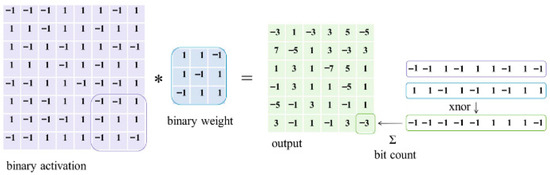
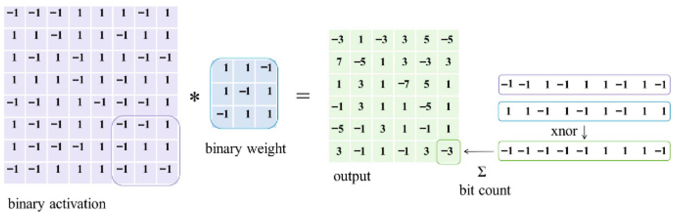
Binary neural networks (BNNs) are a type of quantized model that use binary values (+1 and −1) to represent the weights of convolutional filters and activation values, as shown in Figure 1 [1]. This means that each weight and activation value requires only one bit. In the context of convolutional neural networks (CNNs), which heavily rely on computation speed, BNN models can convert convolution operations into binary multiply–accumulate (BMAC) operations. These operations can be accelerated using highly efficient bitwise computation methods, such as XNOR or population count (Popcnt). Previous research has shown that BNN models can achieve image recognition capabilities that are close to those of full-precision 32-bit models like ResNet [2] and MobileNetV1 [3], indicating a promising future for BNNs. Although BNNs perform calculations using 1-bit weights and activations, there are still floating-point computations during the forward propagation of the model. Floating-point operations (FLOPs) can be a significant burden for embedded platforms, single-chip systems, and microchips with limited computational resources. This study aims to design a more user-friendly neural network model that is suitable for deployment on embedded platforms, edge computing devices and application-specific integrated circuits (ASICs) or system-on-chips (SoCs). By removing the batch normalization (BN) layers [4], this study aims to reduce the floating-point computation load of the model.

2. Related Work

BNNs are a type of deep learning model where the weights of convolutional filters and activation values are binary. Some BNN models binarize activation values into different distributions [5], but, primarily, they are binarized as +1 and −1. This means that each weight and activation value require only one bit to represent, thereby significantly reducing the memory and computational requirements of the model.

2.1. Lightweight Convolutional Model

MobileNetV1 [3] optimizes deep learning for mobile devices by using depthwise separable convolutions, a technique introduced by Xception [6] that splits standard convolution into two stages: depthwise convolution (spatial filtering per channel) and 1 × 1 pointwise convolution (cross-channel feature mixing). This significantly reduces computational costs.

MobileNetV2 [7] improves this by addressing information loss caused by ReLU in low-dimensional spaces. It introduces Inverted Residuals, which expand dimensions before compression (narrow–wide–narrow), reversing the traditional residual block structure to better preserve feature information.

2.2. Optimized BNN Model

2.2.1. BiRealNet Model

BiRealNet [1] enhances BNNs by addressing two primary challenges: limited representational capacity and derivative mismatch. To improve expressiveness, BiRealNet introduces a shortcut pathway that carries real-valued activations to bypass binary convolutions. Since 1-bit kernels provide sparse information, this shortcut preserves critical real-valued data, merging it with binary responses to strengthen the network’s learning capability.

To optimize training, BiRealNet tackles the derivative mismatch problem. Standard BNNs use the Clip, Equation (1), to approximate the non-differentiable Sign function during backpropagation; however, the discrepancy between them hinders convergence. BiRealNet proposes ApproxSign, Equation (2), a second-order approximation function that minimizes this numerical gap, ensuring more accurate gradient updates. In a 1-bit CNN, the real activation, $a_r$, is present during both the training and inference processes, due to convolution.

$$Clip\left(a_r\right)=\left\{\begin{array}{cc}-1\hfill & \hfill if{a}_r<-1\\ a_r\hfill & \hfill if-1\le a_r<1\\ +1\hfill & \hfill otherwise\end{array}\right.,{\displaystyle \frac{\mathsf{\partial }Clip\left(a_r\right)}{\mathsf{\partial }{a}_r}}=\left\{\begin{array}{cc}1\hfill & if-1\le a_r<1\\ 0\hfill & \hfill otherwise\end{array}\right.$$

(1)

$$F\left(a_r\right)=\left\{\begin{array}{c}-1if{a}_r<-1\\ 2a_r+a_r^{2}if-1\le a_r<0\\ 2a_r-a_r^{2}if0\le a_r<1\\ +1otherwise\end{array}\right.,{\displaystyle \frac{\mathsf{\partial }F\left(a_r\right)}{\mathsf{\partial }{a}_r}}=\left\{\begin{array}{c}2+2a_{r}if-1\le a_r<0\\ 2-2a_{r}if0\le a_r<1\\ 0otherwise\end{array}\right.$$

(2)

While BiRealNet significantly narrowed the gap between BNNs and full-precision models—achieving improved accuracy in ResNet architectures—it remains under 60% on ImageNet. This limitation highlights the need for further optimization, a challenge subsequently addressed by ReActNet [8] to achieve even higher performance.

2.2.2. ReActNet Model

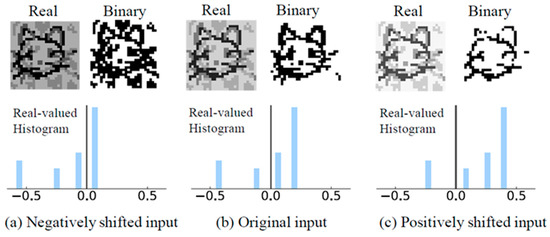
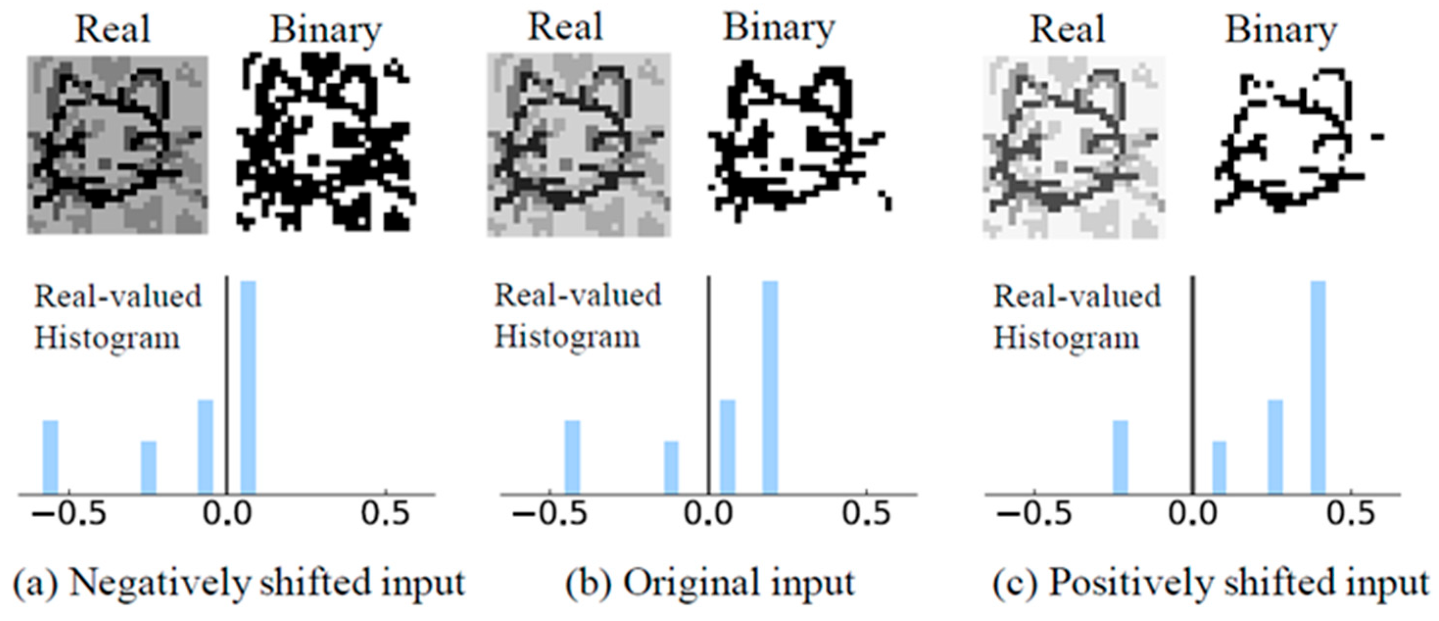
ReActNet highlights that the activation distribution is critical for BNN learning. As shown in Figure 2 [8], binarization can either capture essential features, Figure 2b, or introduce noise and lose information, Figure 2a,c, depending on the alignment of distribution. By shifting the activations to an optimal position before binarization, ReActNet significantly enhances feature learning capabilities. This methodology was successfully integrated into the ResNet and MobileNet backbones to improve performance.

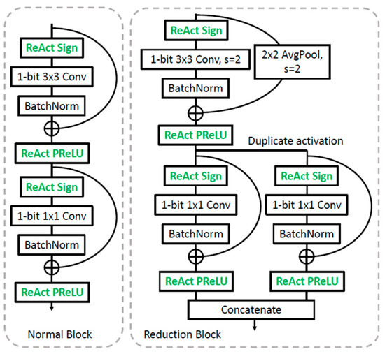
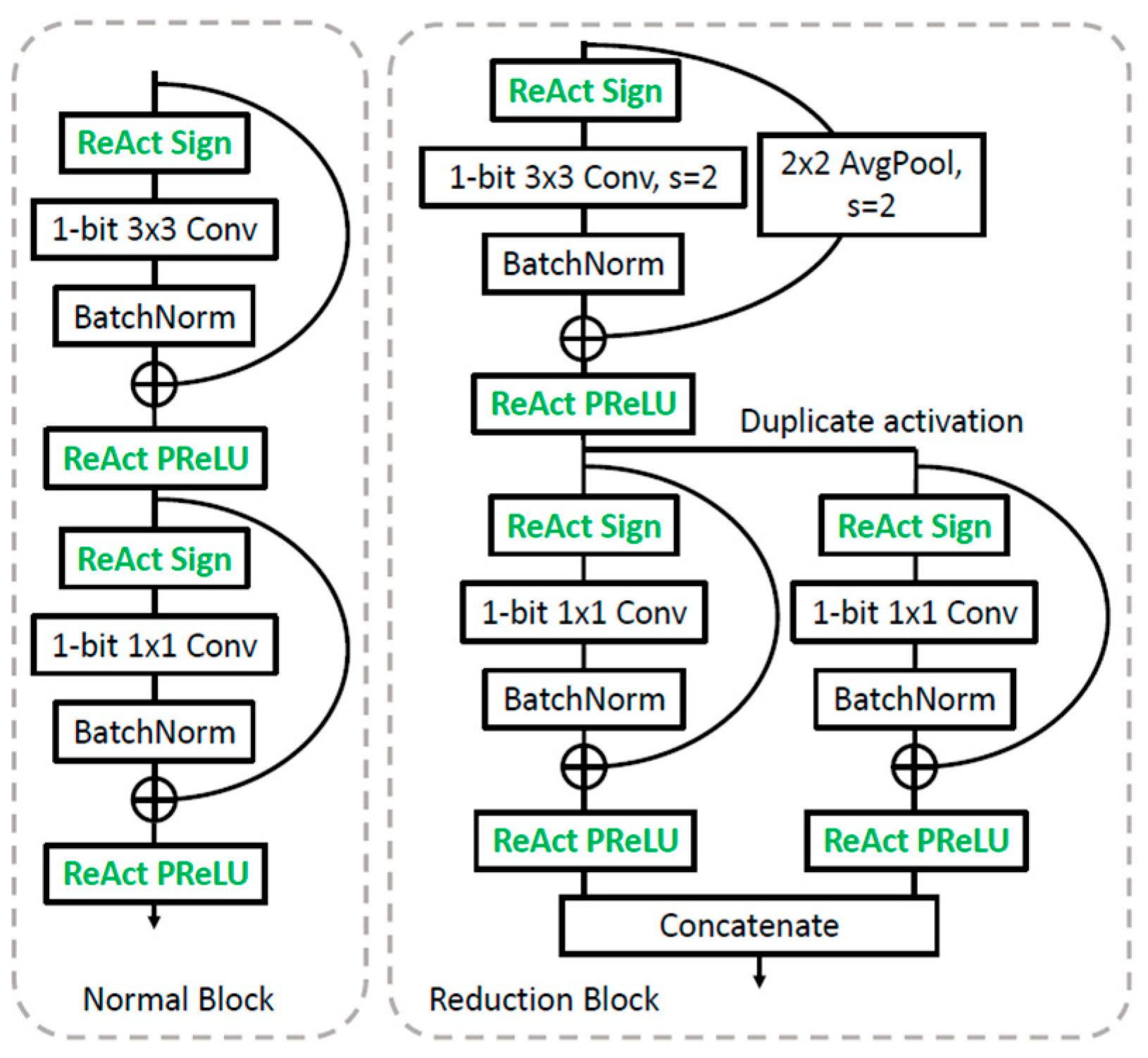
The authors of ReActNet first proposed a baseline model, which is modified based on MobileNet. Unlike MobileNet, it does not use depthwise separable convolutions but uses ordinary 3 × 3 convolutions. The reason is that BNNs have already quantized the convolution computations, so adding depthwise separable convolutions on top of this would degrade the model’s performance. Figure 3 [8] is a model based on this baseline, introduced to optimize the BNN model. These two functions can be applied to any backbone. In this paper, they are only applied to the ResNet and MobileNet models but nevertheless enable the BNN model to achieve 69.4% accuracy on ImageNet—an increase of 13% compared to BiRealNet’s 56.4%, which is nearly approaching the full-precision ResNet model.

In ReActNet, the authors propose RSign and RPReLU to replace the Sign and PReLU in ordinary BNNs. Both of these functions are channel-wise; that is, each channel has its own four parameters—${\alpha }_i$, ${\beta }_i$, ${\gamma }_i$ and ${\zeta }_i$—all of which are learnable, rather than hyperparameters. Equations (3) and (4) are simple linear transformations. RSign uses the ${\alpha }_i$ parameter to dynamically adjust the binarization of the feature maps, while RPReLU uses the ${\beta }_i$, ${\gamma }_i$ and ${\zeta }_i$ parameters to adjust the activations after each convolution. ReActNet mainly leverages these two equations to change the distribution of activations, allowing the BNN model to learn image features more effectively.

$$x_i^b=h\left(x_i^r\right)=\left\{\begin{array}{c}+1if{x}_i^r>{\alpha }_i\\ -1if{x}_i^r\le {\alpha }_i\end{array}\right.$$

(3)

where $x_i^r$ denotes the real-valued input of the RSign function h for the i-th channel. The term $x_i^b$ represents the binary output, while ${\alpha }_i$ is a learnable coefficient that sets the threshold. The subscript i in ${\alpha }_i$ means that the threshold can vary across different channels. The superscripts b and r refer to binary and real values, respectively.

$$f(x_i)=\left\{\begin{array}{cc}{x}_i-{\gamma }_i+{\zeta }_i\hfill & \hfill if{x}_i>{\gamma }_i\\ {\beta }_i(x_i-{\gamma }_i)+{\zeta }_i\hfill & \hfill if{x}_i^r\le {\gamma }_i\end{array}\right.$$

(4)

In the RPReLU function f, $x_i$ represents the input on the i-th channel. The variables ${\gamma }_i$ and ${\zeta }_i$ are learnable shifts that adjust the distribution, while ${\beta }_i$ is a learnable coefficient that controls the slope of the negative part. Each coefficient can vary across different channels.

Since BNN models are quantizations of full-precision models, by reducing the precision of convolutions, we can improve the speed of BNNs. Under this premise, what should we do if we still want to improve the accuracy of BNNs? After proposing the two aforementioned distribution adjustment functions, the authors of ReActNet further propose a distribution loss: namely, knowledge distillation (KD) [9].

2.2.3. FracBNN Model

BNNs evolved as models to better accommodate embedded platforms, yet earlier research rarely designed BNN models specifically for embedded hardware. Fractional activations BNN (FracBNN) [10] is a BNN model that was designed specifically for field-programmable gate array (FPGA) deployment, given that BNNs have 1-bit convolution kernel weights and activations, and FPGAs perform bit operations. BNNs perfectly match the FPGA characteristics, making this model very suitable for FPGA.

FracBNN enhances the representational power of BNN models on FPGA by using 2-bit activations, rather than simply quantizing them to +1 and −1. Furthermore, it employs thermometer encoding to binarize the input layer. In past BNN models, the first convolution layer is typically not binarized, because if the first layer were directly binarized, it would cause a large amount of feature information to be lost at the outset, preventing subsequent convolution layers from learning important features. Hence, a BNN model is not entirely +1 and −1 in its computations; most of the operations are binary, but some remain in full precision.

Previously, we noted that BNN models do not binarize the input in the very first layer when the number of kernels is still small, because if the first layer already loses too much data, the subsequent layers will struggle to learn anything. Therefore, a special encoding method is used to binarize the first layer’s data for accelerated processing. In addition to the first layer, the downsample layer and the final full connection (FC) layer output still remain in full precision in BNNs. The first layer has three input channels for red, green and blue (RGB) colors. If we were to binarize each 8-bit input pixel (0–255) directly, we would lose a large amount of data. Thus, FracBNN uses thermometer encoding, Equation (5) [10]. By increasing the dimensionality, it can binarize without losing so much information. In Equation (5), p represents the pixel value, L represents the dimension of the entire code, i ∈ {1…L}, TV represents the entire encoding and R is used to control the dimensionality after conversion. For example, if R = 32, then 255/32 ≈ 8, so after conversion, you still have 8 bits. In the paper, R is set to 8 to convert to 32 bits, increasing dimensionality and reducing information loss. Here, we use $\mathrm{O}\mathrm{P}\mathrm{s}={\displaystyle \raisebox{1ex}{$BOPs$}\!\left/ \!\raisebox{-1ex}{$64$}\right.}+FLOPs$ [11] to analyze the computational cost of thermometer encoding. Here, FLOPs indicates floating-point operations, BOPs indicates binary operations, and OPs indicates the model’s total computational cost. Suppose the original first layer has three RGB channels, a 32 × 32 input and a 3 × 3 convolution. Then, $\mathrm{O}\mathrm{P}\mathrm{s}={\displaystyle \raisebox{1ex}{$0$}\!\left/ \!\raisebox{-1ex}{$64$}\right.}+3\times 32\times 32\times 3\times 3=\mathrm{27,648}$. If we now set R = 8, converting each input pixel in the RGB channels to 32 bits and using binary operations, $\mathrm{O}\mathrm{P}\mathrm{s}={\displaystyle \raisebox{1ex}{$96\times 32\times 32\times 3\times 3$}\!\left/ \!\raisebox{-1ex}{$64$}\right.}+0=\mathrm{13,824}$. Under the same number of output channels, thermometer encoding can reduce the computational cost to half the original, achieving acceleration.

$$\widetilde{T{V}_i}=\left\{\begin{array}{cc}0\hfill & \hfill 1\le i\le \left[{\displaystyle \frac{255}{R}}\right]-\left[{\displaystyle \frac{p}{R}}\right]\\ 1\hfill & \hfill \left[{\displaystyle \frac{255}{R}}\right]-\left[{\displaystyle \frac{p}{R}}\right]<i\le \left[{\displaystyle \frac{255}{R}}\right]\end{array}\right.$$

(5)

FracBNN does not simply use 1-bit convolution in its computations; instead, it splits the 2 bits into a most significant bit (MSB) and a least significant bit (LSB). By splitting the 2-bit activations into MSB and LSB for separate processing, XNOR and Popcnt can still be used for acceleration. After processing both MSB and LSB, the result from MSB is left-shifted and added to the LSB result. A left shift in binary arithmetic is equivalent to multiplying by two. The LSB has a threshold: only values above that threshold are retained.

3. Methodology

In this section, we will focus on introducing our method and explaining the design principles. First, we will introduce the baseline we adopted. Then, we will discuss the problems encountered when removing the BN layer to reduce the floating-point computation load. To address these issues, we incorporated the scaled weight standardization convolution (WS-Conv) method. We will also explain how to choose the optimizer for BNNs and introduce a series of optimization techniques for the model.

3.1. WSFracBNN Architecture

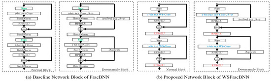
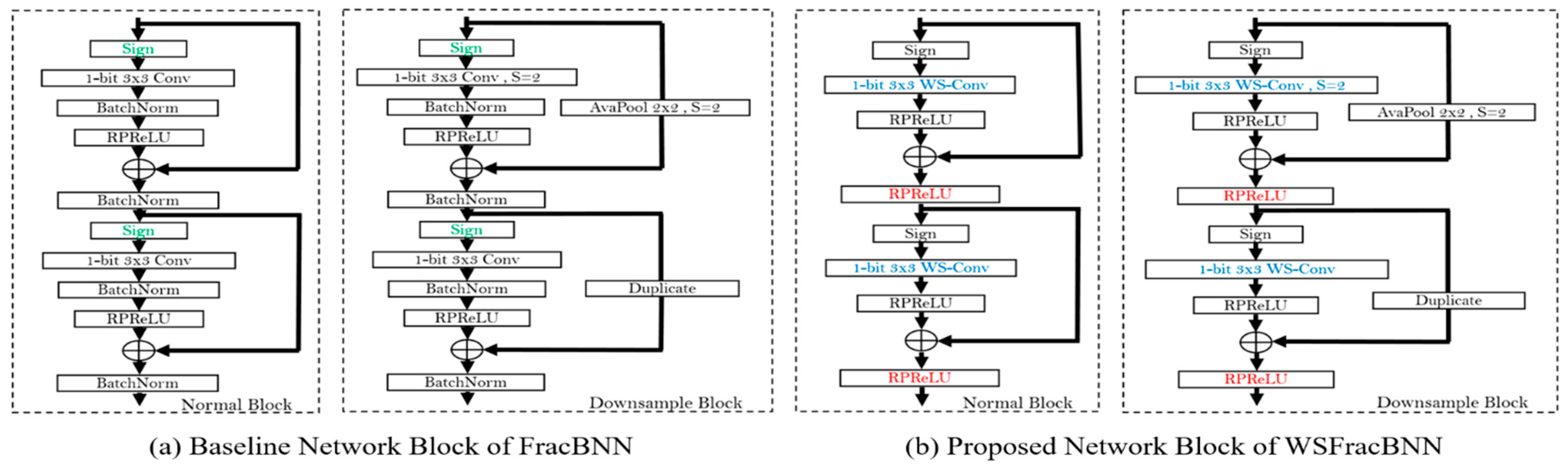
Our baseline is FracBNN, as shown in Figure 4a. Unlike typical BNN models, FracBNN uses 2-bit precision, splitting these 2-bit activation values into 1-bit MSB and 1-bit LSB. Therefore, the convolution operations are still handled with 1-bit convolutions. The backbone used in FracBNN is the ResNet20 model. We chose FracBNN as the baseline because it is a BNN model that is specifically designed for hardware deployment. This paper aims to design a BNN model that is more suitable for embedded platforms. The primary goal in designing a BNN model that is friendly to embedded platforms is to reduce the overall FLOPs of the model.

To address the significant drop in accuracy caused by the absence of the BN layer, we incorporated the scaled WS-Conv method and proposed a new model architecture, as shown in Figure 4b. In this architecture, we removed the BN layer and added the WS-Conv method, as indicated in blue in Figure 4b. Considering the issue of unstable activation values mentioned in ReActNet, we also added RPReLU, as indicated in red in Figure 4b. This paper’s backbone, like FracBNN, uses the ResNet20 architecture. We refer to this model as weight standardization FracBNN, abbreviated as WSFracBNN.

3.2. Scaled Weight Standardization Convolution

BN normalizes the batch input features of each neuron, while weight normalization (WN) normalizes the weights of each neuron. WS-Conv processes each convolution kernel of the weights. It is similar to WNs and offers several advantages over BNs:

• Faster parameter convergence: WS-Conv accelerates the convergence of parameters in deep learning networks by recalculating the weights, W, without the dependency on mini-batches. This makes WS-Conv applicable to recurrent neural networks (RNNs) and long short-term memory networks (LSTMs), whereas BN cannot be directly applied to RNNs and LSTMs.
• Reduced noise: Since WS-Conv recalculates the weights, W, operations based on WS-Conv tend to introduce less noise compared to BN.
• Efficient storage and computation: WS-Conv does not require additional storage for the average and variance of the mini-batch and, additionally, the computational overhead for implementing WS-Conv is minimal. As a result, WS-Conv is generally faster than operations using BN.

To address the mean shift in the distribution of hidden layer activations caused by the absence of BN, we introduced the WS-Conv method. Specifically, we modified all convolutional layers of the baseline model, as shown in Equation (6) [12]:

$${\widehat{W}}_{ij}=\varphi ·{\displaystyle \frac{W_{ij}-{\mu }_i}{\sqrt{N}{\sigma }_i}}$$

(6)

Here, ${\mu }_i$ represents the mean of all convolution kernels, and ${\sigma }_i^2$ represents the variance of all convolution kernels, where ${\mu }_i={\displaystyle \frac{1}{N}}\sum _j{W}_{ij}$, and ${\sigma }_i^2={\displaystyle \frac{1}{N}}\sum _j{(W_{ij}-{\mu }_i)}^2$. The scalar ϕ is used to maintain variance and varies with different activation functions; for ReLU, $\varphi =\sqrt{2/(1-(1/\pi \left)\right)}$. This formula essentially embodies the concept of BN, but while BN processes the activations, WS-Conv processes each convolution kernel of the weights. Compared to processing activations, the number of weights to be processed is much smaller, resulting in only a minor change in FLOPs when applied to the weights.

3.3. Adaptive Gradient Clipping

Adaptive gradient clipping (AGC) was introduced to address the issue of gradients exploding. Traditionally, gradient clipping is used to limit the range of gradients, thereby stabilizing the training process [13]. Before updating the gradients, the clipping is performed using Formula (7)

$$\mathrm{G}⟶\left\{\begin{array}{c}\lambda {\displaystyle \frac{G}{‖G‖}}if‖G‖>\lambda ,\\ GOtherwise.\end{array}\right.$$

(7)

where the gradient vector G = ${\displaystyle \raisebox{1ex}{$\mathsf{\partial }\mathrm{L}$}\!\left/ \!\raisebox{-1ex}{$\mathsf{\partial }\mathsf{\theta }$}\right.}$, L is the loss, θ is the parameter vector and λ is the clipping threshold, which is a hyperparameter that needs to be adjusted. A normalizer-free net (NFNet) [12] identified issues with gradient clipping that could lead to instability during training and proposed AGC to improve the performance of normalizer-free ResNet (NF-ResNet) [14]. AGC is based on the norm ratio between the gradients and the convolutional kernel weights, as shown in Formula (8).

$$\begin{gathered} {\mathrm{G}}_i^{\mathcal{l}}⟶\left\{\begin{array}{c}\lambda {\displaystyle \frac{{‖{\mathrm{W}}_i^{\mathcal{l}}‖}_F^{\star }}{{‖{\mathrm{G}}_i^{\mathcal{l}}‖}_F}}{\mathrm{G}}_i^{\mathcal{l}}if{\displaystyle \frac{{‖{\mathrm{G}}_i^{\mathcal{l}}‖}_F}{{‖{\mathrm{W}}_i^{\mathcal{l}}‖}_F^{\star }}}>\lambda ,\\ {\mathrm{G}}_i^{\mathcal{l}}Otherwise.\end{array}\right. \\ {‖{\mathrm{W}}_i^{\mathcal{l}}‖}_F^{\star }=\max \left({‖{\mathrm{W}}_i^{\mathcal{l}}‖}_F,ϵ\right) \end{gathered}$$

(8)

Here, $ϵ={10}^{-3}$ is used to prevent zero-initialized parameters from always being clipped to zero, ${\mathrm{G}}_i^{\mathcal{l}}$ represents the i-th row of the gradient matrix, ${\mathrm{W}}_i^{\mathcal{l}}$ represents the i-th row of the weight matrix, $\mathcal{l}$ denotes the layer of the network, ${‖\cdot ‖}_F$ is the Frobenius norm and λ is the clipping threshold, which is a hyperparameter that needs to be adjusted.

3.4. Knowledge Distillation

Knowledge distillation (KD) is a model compression technique. When BNNs quantize the original network to 1-bit, the accuracy inevitably decreases. To make the accuracy of the quantized model as close as possible to the original full-precision model, knowledge distillation [15] was introduced. Knowledge distillation is a teacher–student training method, where the student model learns from a more complex teacher model. The knowledge distillation loss used in this paper is formulated as Equation (9) [8].

$${\mathcal{L}}_{Distribution}=-{\displaystyle \frac{1}{n}}\sum _c\sum _{i=1}^n{p}_c^{{\mathcal{R}}_{\theta }}\left(X_i\right)\mathrm{l}\mathrm{o}\mathrm{g}({\displaystyle \frac{p_c^{{\mathcal{B}}_{\theta }}\left(X_i\right)}{p_c^{{\mathcal{R}}_{\theta }}\left(X_i\right)}})$$

(9)

where the distributional loss, $\mathcal{L}$_Distribution, is defined as the Kullback–Leibler (KL) divergence between the softmax output, p_c, of a real-valued network, R_θ, and that of a binary network, B_θ. The subscript, c, represents different classes, while n denotes the batch size.

During training, we hope the BNN model can learn a distribution and parameters that are similar to those of a full-precision model, so that the BNN approximates the full-precision model more closely. Thus, the loss function in Equation (9) was proposed. With this training approach, BNN performance can be improved even further. Unlike previous training methods [11] that require matching the output of each layer or using multi-step structures [16], this loss is simpler to use and can still achieve good results. Additionally, since it does not require matching the output of each layer, it allows for more flexibility in choosing the teacher model. The teacher model used in this paper is NFNet-F0 [11].

4. Experiments

4.1. Experiment Enviroment

This study’s proposed architecture is primarily developed in the Python language, using the PyTorch deep learning framework, and is trained and tested on an NVIDIA GeForce RTX 3090 Ti graphics card. The detailed hardware and software environment are shown in

Table 1. Experimental hardware equipment environment.

CPU	Intel@ CoreTM i9-12900K
GPU	NVIDIA GeForce RTX 3090Ti
GPU Memory	24 GB
Memory	16 GB

and

Table 2. Software environment.

OS	Ubuntu 20.04.6 LTS
Python	2.7.18
PyTorch	2.0.1
Torch	2.0.1+cu117
Torchvision	0.15.2+cu117

.

4.2. Datasets

The datasets used in this thesis are CIFAR-10 [17] and CIFAR-100, provided by the Canadian Institute for Advanced Research (CIFAR). CIFAR-10 consists of 60,000 32 × 32 color images from 10 classes. CIFAR-10 is a relatively small dataset, while CIFAR-100 is an extended version of CIFAR-10. Unlike CIFAR-10, CIFAR-100 contains 100 classes, which are grouped into 20 superclasses, with each superclass containing 5 subclasses. Both datasets are divided into 50,000 training images and 10,000 test images. These datasets are mainly used for image classification tasks. CIFAR-100 is more challenging to train because, despite the small image size of 32 × 32, it contains 100 classes.

4.3. Training Strategy

When training BNNs, a two-stage training method [16] is typically used to achieve better results. This training strategy breaks down the training process into two specific stages. In the first stage, the activations of the model are binarized. Typically, the activations of each layer are binarized to +1 and −1, using the Sign function, while the weights remain in 32-bit full precision during this phase of training. In the second stage, we fine-tune the model trained in the first stage, binarizing both the weights and the activations. During this stage, we set the weight decay to zero and continue training the model. In this paper, we use Adam [18] as the optimizer for both stages of training and employ KD to train the teacher and student models together. The student model is the WSFracBNN model, and the teacher model is a normalizer-free net, NFNet-F0.

4.4. Optimizer Selection

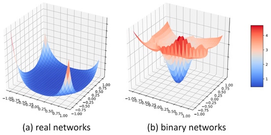
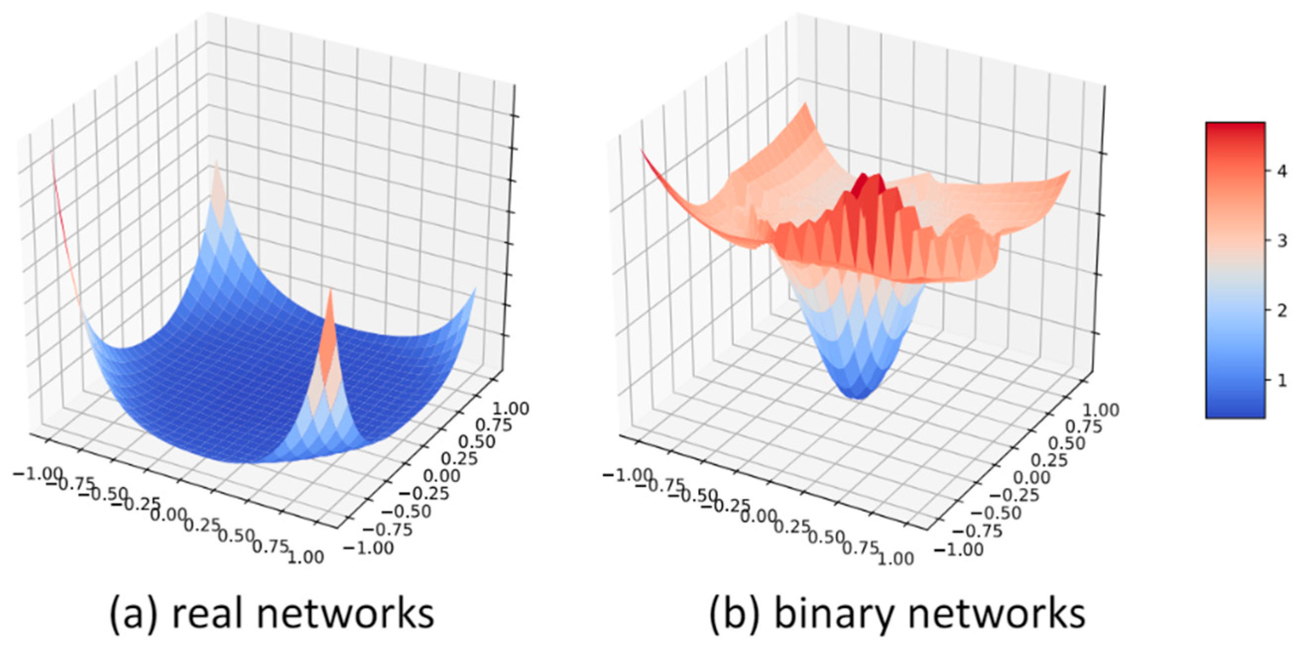
BNNs are models that binarize both convolution kernel weights and activations. So, how should one choose an optimizer for them? In previous papers, Adam is usually used, as well as multi-step training methods, to optimize BNN models (e.g., [11,14]). However, few studies investigate why Adam is superior to other optimizers (such as stochastic gradient decent (SGD)) when training BNN models. The paper [5] gives us a good direction—refer to Figure 5 [5]. The optimization surface of a full-precision model near a local minimum is smoother, as shown in Figure 5a, thus making it easier to generalize the training results to the testing results. In contrast, the local optimization surface near a local minimum for BNNs is more rugged, making optimization more difficult, as shown in Figure 5b. Therefore, even though they are both image classification tasks, the choice of optimizer for a BNN model is different.

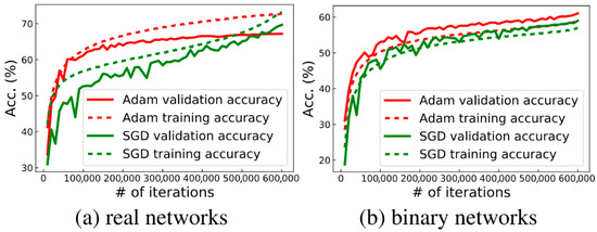
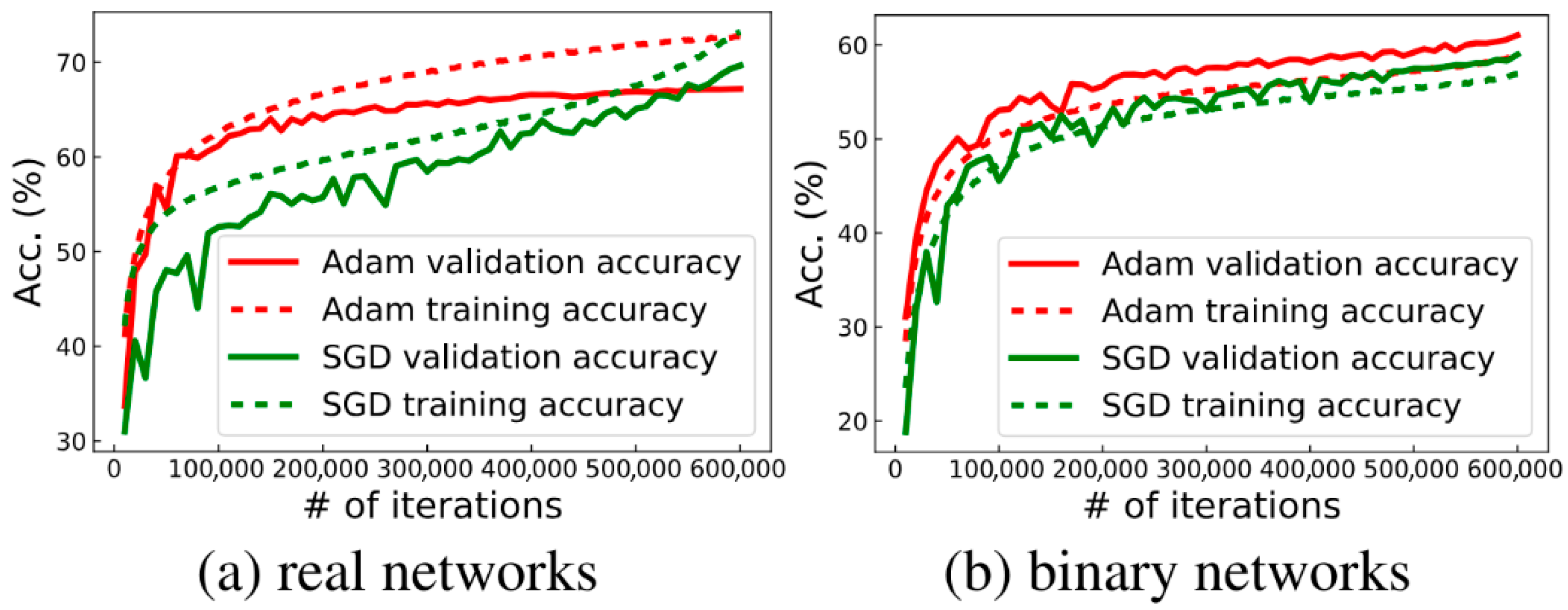
In Figure 6a [5], it can be observed that the SGD optimizer is quite powerful for training full-precision models, which is why almost all image classification models now use SGD. But this is not the case for BNN models. Because BNNs are small models that are extremely quantized, they easily underfit on the training set, even if more iterations are used. In Figure 6b [5], compared to Adam, the validation accuracy of BNNs trained with SGD fluctuates more. This indicates that when training BNNs, SGD easily falls into the rugged surface of optimizing discrete convolution kernel weights, while Adam can find a better global minimum during training, leading to better convergence for BNN models.

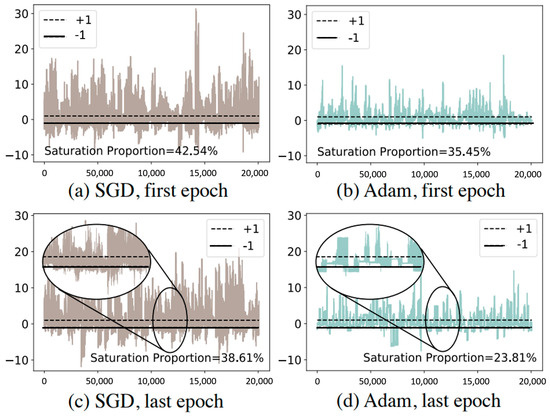
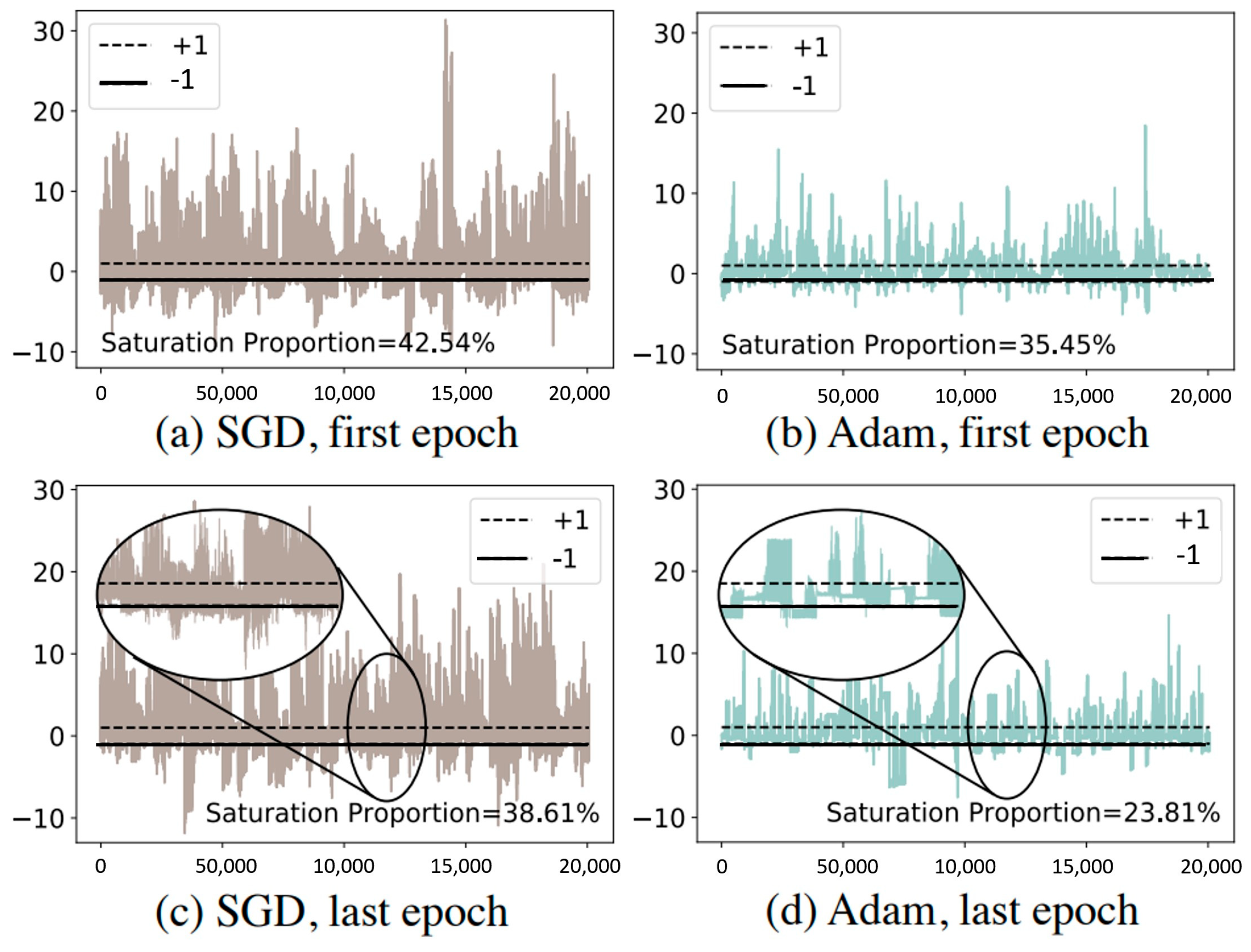
Why is Adam easier for training BNN models? This must be explained from the perspective of BNN characteristics. BNN models require binarizing both convolution kernel weights and activations to +1 and −1; thus, BNNs need to quantize all their parameters, using the Sign function. As introduced in Section 2.2.1, the Sign function is non-differentiable, so the Clip function is used to approximate it during backpropagation. This triggers a common BNN problem: when the activations of the previous layer in BNNs exceed the range of +1 and −1, activation saturation occurs, and the corresponding derivative value becomes 0, leading to the dreadful vanishing gradient problem. In the visualization of Figure 7 [5], one can observe that it is very common for the activations in BNNs to exceed the +1 and −1 range. Hence, the gradient vanishes due to over-saturated activations, so the parameters do not receive enough gradients to learn and tend to become stuck in a local minimum. This is a very important issue in BNN optimization. From the visualization in Figure 7a,c, it can be seen that SGD easily results in activation saturation when optimizing BNNs. Meanwhile, from Figure 7b,d, one can see that in Adam optimization, the issues of activation saturation and vanishing gradients are mitigated.

The SGD optimizer updates parameters according to Equation (10).

$$\mathrm{S}\mathrm{G}\mathrm{D}:v_t=v_{t-1}+\left(1-\phi \right)g_t$$

(10)

where $g_t$ denotes the gradient and $v_t$ denotes the first-moment weight update. $\phi$ is the decay rate of the first moment (commonly set to 0.9). This optimization method only calculates the first moment. When encountering vanishing gradients, the corresponding weight updates drop rapidly.

Adam performs optimization through Equation (11),

$$\begin{gathered} \mathrm{A}\mathrm{d}\mathrm{a}\mathrm{m}:u_t={\displaystyle \frac{\widehat{v_t}}{\sqrt{\widehat{m_t}}+ϵ}} \\ \widehat{m_t}={\displaystyle \frac{m_t}{1-{\eta }_1^t}},m_t={\eta }_1{m}_{t-1}+\left(1-{\eta }_1\right)g_t \\ \widehat{v_t}={\displaystyle \frac{v_t}{1-{\eta }_2^t}},v_t={{\eta }_2{v}_{t-1}+(1-{\eta }_2)g}_t^2 \end{gathered}$$

(11)

where $g_t$ is the gradient, $m_t$ is the first moment and ${\eta }_1$ is the decay rate of the first moment. $v_t$ is the second moment and ${\eta }_2$ is the decay rate of the second moment. $\widehat{m_t}$ and $\widehat{v_t}$ are used to eliminate the bias of the first and second moments at the beginning, and $ϵ$ is a small constant (usually set to ${10}^{-8}$ to prevent division by zero). In Adam, the second moment is accumulated, thereby amplifying the learning rate in the directions of the vanishing gradients and increasing the weight update in those directions. This helps the network to overcome local minima and achieve a better solution. Hence, Adam surpasses SGD in BNN optimization.

4.5. Testing WSFracBNN on CIFAR-100

We did not train and test our designed WSFracBNN on ImageNet [9]. Given the limited hardware resources at hand, we chose to train and test it on the CIFAR-100 dataset. We did not pre-train it on ImageNet but trained it from scratch on CIFAR-100. During training, we directly used images of size 32 × 32 and applied only basic data augmentation methods such as horizontal flipping. For training WSFracBNN, we used a two-stage training procedure, employing Adam as the optimization algorithm in both stages.

In the first stage, we only binarized the activations, setting the learning rate to 1 × 10⁻³, weight decay to 5 × 10⁻⁴, batch size to 128 and training for 250 epochs. In the second stage, both activations and convolutional kernel weights were binarized, with a stepwise learning rate strategy: starting at 1 × 10⁻³, then reducing to 1 × 10⁻⁴ after 100 epochs, to 1 × 10⁻⁵ after 150 epochs and finally to 1 × 10⁻⁶ at 200 epochs, continuing training until 250 epochs. The weight decay was set to 0 in the second stage.

Additionally, we incorporated AGC and KD methods. For AGC, we set the hyperparameter $\lambda$ for adaptive gradient clipping to 1 × 10⁻⁴ in both stages. For KD, the teacher model in both stages was an NFNet model.

Table 3. Comparison of WSFracBNN with other models on CIFAR-100. *BL represents baseline.

Network	Top-1 Acc (%)	FLOPs $(\times {10}^6$)	BOPs $(\times {10}^9$)	OPs $(\times {10}^8$)
MobileNetV2	62.1	2462	0	24.6
FracBNN (*BL)	58.9	84.3	4.62	1.56
ReActNet-A	52.7	25.3	4.83	1.01
BiRealNet-18	51.8	12.4	1.81	0.4
WSFracBNN (Our)	59.5	0.06	4.62	0.73 (↓54%)

shows the performance of our model on CIFAR-100 in our experimental setup. FLOPs represents floating-point operations, BOPs represents binary operations, and OPs represents the total operations of the BNNs model, calculated as $OPs={\displaystyle \raisebox{1ex}{$BOPs$}\!\left/ \!\raisebox{-1ex}{$64$}\right.}+FLOPs$.

Our WSFracBNN model significantly reduced FLOPs to nearly zero while maintaining almost the same BOPs, achieving an accuracy of 59.5%, which is 0.6% higher than the baseline FracBNN model. This accuracy is only 2.6% lower than that of the full-precision MobileNetV2 and surpasses the well-known BiRealNet-18 and ReActNet-A by 7.7% and 6.8%, respectively. The total operations (OPs) of our model are only 46% of those of the baseline model. It means that the total OPs of our model is reduced by 54% compared to the baseline. Although the OPs of WSFracBNN are not lower than those of BiRealNet-18, WSFracBNN still has a better trade-off between accuracy and computational cost.

4.6. Performance Efficiency Analysis on CPU

The speed metric, throughput, which measures the number of images a model can process per unit of time, becomes a crucial factor in evaluating the model’s practicality. Therefore, we conducted an in-depth speed performance evaluation of our proposed WSFracBNN model, as shown in

Table 4. Speed analysis of BNNs models on the CPU. *BL represents baseline.

Binary Network	Input Size (Pixel)	Throughput (img/s)
FracBNN (*BL)	$32\times 32$	66,181
ReActNet-A	$32\times 32$	54,894
BiRealNet-18	$32\times 32$	215,007
WSFracBNN (Our)	$32\times 32$	73,287

, to verify its feasibility in real-world applications. To objectively assess the model’s performance, we compared WSFracBNN with a series of well-known BNNs models. These models include FracBNN, ReActNet-A and BiRealNet-18. The results show that removing the BN layer can reduce the model’s complexity and computational requirements, making the model more suitable for edge computing devices.

In our experimental setup, all models were tested on the same CPU. Table 4 shows that our model has certain advantages in resource-constrained environments. WSFracBNN not only outperformed FracBNN and ReActNet-A in processing speed but also approached the performance of BiRealNet-18. Although BiRealNet-18 achieved a significant advantage in speed, it did so at the expense of accuracy. Furthermore, after removing the BN layer, the WSFracBNN model not only reduced the computational load but also demonstrated efficient CPU performance. This means that our WSFracBNN model strikes a better balance between the computational load, execution efficiency and accuracy compared to FracBNN, ReActNet-A and BiRealNet-18, making it more suitable for deployment on small chips or other embedded platforms.

4.7. Ablation Study

The clipping threshold, $\lambda$, plays a crucial role in the effectiveness of AGC. Through experiments, we analyzed how the threshold affects the training process and final performance. As shown in

Table 5. The impact of clipping threshold λ in adaptive gradient clipping on WSFracBNN performance on CIFAR-10 and CIFAR-100.

$\mathit{\lambda }$	Cifar10	Cifar100
w/o AGC	87.3	56.5
$1\times {10}^{-2}$	87.5	56.1
$5\times {10}^{-3}$	87.3	57.8
$1\times {10}^{-3}$	87.5	58.6
$1\times {10}^{-4}$	87.4	58.9

, the results indicate that using an appropriate threshold can achieve an additional 1% to 2.4% accuracy improvement on CIFAR-100. Furthermore, the performance without the BN layer on CIFAR-10 is minimally affected by the clipping value. The main possible explanation is that CIFAR-10 classification is overly simple, with performance already nearing saturation and being less sensitive. However, we found that when the threshold in AGC is extremely large, the training process becomes less stable. We believe this is primarily due to the instability caused by excessively extreme gradient clipping.

We employed the knowledge distillation method to enhance the performance of the student model by allowing the student model, WSFracBNN, to learn from a more complex teacher model. We compared the two teacher models, ResNet-34 and NFNet-F0, that were used to train WSFracBNN on the CIFAR-100 dataset. As shown in

Table 6. Comparison of teacher model selection for training WSFracBNN on CIFAR-100.

Teacher Model	WSFracBNN Top-1 Acc (%)
w/o Teacher	56.5
ResNet-34	57.9
NFNet-F0	58.8

, “w/o teacher model” represents training with CrossEntropyLoss. NFNet-F0 slightly outperformed ResNet-34 in terms of accuracy on CIFAR-100. We believe that NFNet-F0 may be more effective as a teacher model, because its structure is more similar to that of WSFracBNN, enabling the student model to better learn the distribution from NFNet-F0 on complex datasets.

During the knowledge distillation process, the student model not only learns to predict the correct classes better but also mimics the behavior and output distribution of the teacher model. This typically includes learning the teacher model’s Softmax outputs to gain richer information and guidance, thereby improving its own prediction accuracy. This method is particularly important for BNN models, as their expressive capability is limited. Through distillation, the depth and detail of the model’s learning can be effectively supplemented.

We gradually incorporated the WS-Conv, AGC, and KD loss methods into WSFracBNN. As shown in

Table 7. Ablation study of WS-Conv, AGC and KD loss on WSFracBNN in CIFAR-100.

Setting	WSFracBNN Top-1 Acc (%)
-	39.0
+WS-Conv	56.5
+AGC	58.9
+KD Loss	59.6

, starting with no methods added and without the BN layer, the model achieved only 39% accuracy on the CIFAR-100 dataset. When we first added the WS-Conv method, which processes the weights, the accuracy improved from 39% to 56.5%: an increase of 17.5%. This demonstrates the importance of WS-Conv for the model.

Next, we found that training the BNN model using only the WS-Conv method resulted in unstable performance on the CIFAR-100 dataset. Therefore, we additionally incorporated the AGC method during training. By using the ratio of the gradient to the weight, the instability during training was addressed, improving the accuracy from 56.5% to 58.9%, an increase of 2.4%, reaching the baseline accuracy on CIFAR-100.

Finally, we introduced the knowledge distillation method using the KD loss formula. As shown in Table 7, NFNet-F0 was selected as the teacher model for training. This improved the accuracy from 58.9% to 59.5%, an increase of 0.6%, successfully surpassing the baseline by 0.6%. This demonstrates that each method we added was effective for our model and successfully reflected in the accuracy improvement.

5. Conclusions

We proposed a hardware-friendly BNNs model in this study. Understanding the importance of BN to the model, we also identified its drawbacks, which affect model inference and are unfriendly to embedded platforms. By removing the BN layer, the proposed model reduced the FLOPs of the baseline model, FracBNN, to almost zero. Moreover, without changing the BOPs, the accuracy on CIFAR-100 improved by 0.6% compared to the baseline model.

Compared to FracBNN, the proposed model offers four main advantages. First, it eliminates BN layers, which reduces the number of floating-point operations. Second, it introduces scaled WS-Conv to mitigate the significant accuracy drop that typically occurs without BN layers. Third, it incorporates AGC to prevent exploding gradients during the training stage and to allow the model to be trained stably. Finally, it utilizes KD to ensure that the accuracy of the quantized model remains as close as possible to that of the original full-precision model. In addition, in comparison to other BN-free approaches, the proposed model retains the aforementioned benefits, excluding the first one.

References

- Liu, Z.; Wu, B.; Luo, W.; Yang, X.; Liu, W.; Cheng, K.T. Bi-real net: Enhancing the performance of 1-bit cnns with improved representational capability and advanced training algorithm. In Proceedings of the European Conference on Computer Vision (ECCV), Munich, Germany, 8–14 September 2018; pp. 722–737. [Google Scholar]
- Krizhevsky, A.; Hinton, G. Convolutional deep belief networks on cifar-10. Unpubl. Manuscr. 2010, 40, 1–9. [Google Scholar]
- Liu, Z.; Shen, Z.; Li, S.; Helwegen, K.; Huang, D.; Cheng, K.T. How do adam and training strategies help bnns optimization. In Proceedings of the International Conference on Machine Learning, PMLR, Virtual, 18–24 July 2021; pp. 6936–6946. [Google Scholar]
- Zhang, Y.; Pan, J.; Liu, X.; Chen, H.; Chen, D.; Zhang, Z. FracBNN: Accurate and FPGA-efficient binary neural networks with fractional activations. In Proceedings of the 2021 ACM/SIGDA International Symposium on Field-Programmable Gate Arrays, Virtual, 28 February–2 March 2021; pp. 171–182. [Google Scholar]
- Sandler, M.; Howard, A.; Zhu, M.; Zhmoginov, A.; Chen, L.C. Mobilenetv2: Inverted residuals and linear bottlenecks. In Proceedings of the IEEE Conference on Computer Vision and Pattern Recognition, Salt Lake City, UT, USA, 18–23 June 2018; pp. 4510–4520. [Google Scholar]
- He, K.; Zhang, X.; Ren, S.; Sun, J. Deep residual learning for image recognition. In Proceedings of the IEEE Conference on Computer Vision and Pattern Recognition, Las Vegas, NV, USA, 27–30 June 2016; pp. 770–778. [Google Scholar]
- Liu, Z.; Shen, Z.; Savvides, M.; Cheng, K.T. Reactnet: Towards precise binary neural network with generalized activation functions. In Proceedings of the Computer Vision–ECCV 2020: 16th European Conference, Glasgow, UK, 28 August 2020; Proceedings, Part XIV 16. Springer International Publishing: Berlin/Heidelberg, Germany, 2020; pp. 143–159. [Google Scholar]
- Brock, A.; De, S.; Smith, S.L. Characterizing signal propagation to close the performance gap in unnormalized resnets. arXiv 2021, arXiv:2101.08692. [Google Scholar] [CrossRef] [Scilit]
- Howard, A.G.; Zhu, M.; Chen, B.; Kalenichenko, D.; Wang, W.; Weyand, T.; Andreetto, M.; Adam, H. Mobilenets: Efficient convolutional neural networks for mobile vision applications. arXiv 2017, arXiv:1704.04861. [Google Scholar] [CrossRef] [Scilit]
- Deng, J.; Dong, W.; Socher, R.; Li, L.J.; Li, K.; Fei-Fei, L. Imagenet: A large-scale hierarchical image database. In Proceedings of the 2009 IEEE Conference on Computer Vision and Pattern Recognition, Miami, FL, USA, 20–25 June 2009; pp. 248–255. [Google Scholar]
- Tu, Z.; Chen, X.; Ren, P.; Wang, Y. Adabin: Improving binary neural networks with adaptive binary sets. In Proceedings of the European Conference on Computer Vision, Tel Aviv, Israel, 23–27 October 2022; Springer Nature: Cham, Switzerland, 2022; pp. 379–395. [Google Scholar]
- Chollet, F. Xception: Deep learning with depthwise separable convolutions. In Proceedings of the IEEE Conference on Computer Vision and Pattern Recognition, Honolulu, HI, USA, 21–26 July 2017; pp. 1251–1258. [Google Scholar]
- Merity, S.; Keskar, N.S.; Socher, R. Regularizing and optimizing LSTM language models. arXiv 2017, arXiv:1708.02182. [Google Scholar] [CrossRef] [Scilit]
- Zhuang, B.; Shen, C.; Tan, M.; Liu, L.; Reid, I. Towards effective low-bitwidth convolutional neural networks. In Proceedings of the IEEE Conference on Computer Vision and Pattern Recognition, Salt Lake City, UT, USA, 18–23 June 2018; pp. 7920–7928. [Google Scholar]
- Brock, A.; De, S.; Smith, S.L.; Simonyan, K. High-performance large-scale image recognition without normalization. In Proceedings of the International Conference on Machine Learning, PMLR, Virtual, 18–24 July 2021; pp. 1059–1071. [Google Scholar]
- Martinez, B.; Yang, J.; Bulat, A.; Tzimiropoulos, G. Training binary neural networks with real-to-binary convolutions. arXiv 2020, arXiv:2003.11535. [Google Scholar]
- Hinton, G.; Vinyals, O.; Dean, J. Distilling the knowledge in a neural network. arXiv 2015, arXiv:1503.02531. [Google Scholar] [CrossRef] [Scilit]
- Ioffe, S.; Szegedy, C. Batch normalization: Accelerating deep network training by reducing internal covariate shift. In Proceedings of the International Conference on Machine Learning, PMLR, Lille, France, 7–9 June 2015; pp. 448–456. [Google Scholar]
Disclaimer/Publisher’s Note: The statements, opinions and data contained in all publications are solely those of the individual author(s) and contributor(s) and not of MDPI and/or the editor(s). MDPI and/or the editor(s) disclaim responsibility for any injury to people or property resulting from any ideas, methods, instructions or products referred to in the content. |
© 2026 by the authors. Licensee MDPI, Basel, Switzerland. This article is an open access article distributed under the terms and conditions of the Creative Commons Attribution (CC BY) license.