


Abstract
In the Internet of Things (IoT), ultra-wideband (UWB) plays an essential role in localization and navigation. However, in indoor environments, UWB signals are often blocked by obstacles, leading to non-line-of-sight (NLOS) propagation. Thus, reliable line-of-sight (LOS)/NLOS identification is essential for reducing errors and enhancing the robustness of localization. This paper focuses on a single-anchor UWB configuration and proposes a temporal deep learning framework that jointly exploits two-way ranging (TWR) and angle-of-arrival (AOA) measurements for LOS/NLOS identification. At the core of the model is a temporal convolutional network (TCN) augmented with a self-attentive pooling mechanism, which enables the extraction of dynamic propagation patterns and temporal contextual information. Experimental evaluations on real-world measurement data show that the proposed method achieves an accuracy of 96.65% on the collected dataset and yields accuracies ranging from 88.72% to 93.56% across the three scenes, outperforming representative deep learning baselines. These results indicate that jointly exploiting geometric and temporal information in a single-anchor configuration is an effective approach for robust UWB indoor positioning.
1. Introduction
Reliable indoor localization and navigation have emerged as indispensable elements for modern Internet of Things (IoT)-enabled environments [1]. Global navigation satellite systems are not suitable for indoor use due to signal attenuation, blockage, and multipath propagation [2]. To fulfill these requirements, indoor positioning systems (IPSs) that rely on wireless infrastructures, including Wi-Fi, Bluetooth, visible light communication (VLC), magneto-inductive systems, and ultra-wideband (UWB), have been developed. Among these technologies, UWB is well suited to infrastructure-constrained indoor localization. Its large bandwidth enables accurate time-of-flight (ToF) ranging on commodity transceivers, and in dual-antenna designs, UWB radios can further provide phase-difference-of-arrival (PDOA)-derived AOA, enabling combined ranging and AOA observations even in a single-anchor deployment [3,4,5]. In contrast, Wi-Fi and Bluetooth rely on RSS/CSI fingerprinting or multi-anchor ranging, whereas VLC systems typically impose stricter hardware, line-of-sight, or environmental constraints [6,7]. Magneto-inductive systems have also been explored for localization in occluded media, but they are typically limited by near-field magnetic coupling and coil-based hardware requirements [8].
UWB has been widely adopted for indoor localization owing to its large bandwidth, low power consumption, centimeter-level positioning accuracy, and the ability to coexist with other radio systems under low-power spectral density constraints [9]. These properties make UWB particularly suitable for infrastructure-constrained settings, where commodity transceivers can provide direct physical observables such as double-sided two-way ranging (DS-TWR) ranging and PDOA-derived angle measurements with minimal deployment overhead. However, despite these advantages, indoor UWB links are often affected by non-line-of-sight (NLOS) propagation through walls, furniture, or temporary obstructions. NLOS conditions typically introduce systematic positive ranging bias and increased uncertainty, which can severely degrade localization accuracy and robustness [10]. Therefore, reliable LOS/NLOS identification is widely regarded as a prerequisite for effective NLOS mitigation and robust UWB positioning [11].
Existing LOS/NLOS identification methods can be broadly categorized by the type of observables: channel-information-driven approaches that exploit raw waveform-level measurements, and measurement-driven approaches that operate on readily available physical measurements from commodity devices [12]. Channel-level methods can be highly discriminative in-domain but often require high-rate raw-signal access, incur nontrivial storage/latency overhead, and may exhibit sensitivity to hardware and scene shifts. In contrast, measurement-driven methods are easier to deploy on off-the-shelf transceivers, yet many of them still rely on handcrafted statistics or thresholds and may have limited capability to exploit temporal evidence under dynamic motion. These limitations become more pronounced in infrastructure-constrained settings, where single-anchor configurations are desirable for cost and deployment simplicity but are more vulnerable to NLOS-induced bias and temporal instability.
Based on these issues, this paper investigates LOS/NLOS identification in a single-anchor UWB system, where one stationary anchor exchanges DS-TWR messages with one mobile tag and reports a time series of TWR ranges and PDOA-derived AOA measurements. The objective is to determine the visibility state of the single anchor–tag link by exploiting temporal range–angle characteristics under constrained infrastructure. To this end, we develop a deep temporal model that jointly learns discriminative representations from the range sequence and the sine–cosine encoded AOA sequence. A controlled experimental campaign is conducted in indoor environments, where static obstacles are arranged to generate LOS and NLOS conditions for data acquisition and evaluation. The proposed approach aims to improve classification accuracy while retaining a single-anchor deployment.
The main contributions of this paper are summarized as follows:
- A single-anchor temporal convolutional network (TCN) with attention is created to jointly model single-anchor distance and angle sequences. The design includes dilated residual convolutions, temporal self-attention, and global pooling to capture multiscale time patterns.
- On a single-anchor UWB dataset collected experimentally, systematic experiments are performed. Results demonstrate the classification performance, temporal-scale robustness, and practical applicability of the proposed network for LOS/NLOS identification.
The remainder of this paper is organized as follows. Section 2 reviews related work on UWB LOS/NLOS identification, covering both channel-driven and measurement-driven approaches. Section 3 presents the proposed RA-TCN framework, including feature construction, network design, and the training strategy. Section 4 describes the UWB hardware, the experimental setup, the data collection protocol, and the statistical analysis of the measured range and PDOA signals. Section 5 reports the experimental results, including model comparisons, cross-scene generalization, robustness to window length, ablation studies, and a discussion of performance factors and error cases. Section 6 concludes the paper and outlines the limitations and future directions.
1.1. Background and Problem Formulation
1.1.1. UWB Ranging Principle
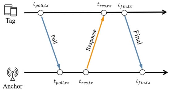
This paper adopts a DS-TWR scheme. In DS-TWR, the tag and anchor exchange a sequence of ranging messages and record the transmit/receive timestamps at both ends. Through these timestamps, the scheme eliminates the unknown clock offset between the two devices, enabling an accurate estimate of the one-way time of flight. This time estimate is then converted into the propagation distance between the devices.
As illustrated in Figure 1, DS-TWR performs distance estimation using a three-message handshake comprising poll, response, and final messages. An optional report frame collects all timestamps at a single endpoint for subsequent computation. During the exchange, each device generates timestamp reports for transmit and receive events at the antenna port. The time reference for these reports is the ranging marker, defined as the instant when the first symbol of the physical layer header of the ranging frame arrives at the local antenna.
Figure 1.
Distance estimation based on double-sided two-way ranging (DS-TWR).
Let and denote the round-trip times measured in the two directions, and let and denote the corresponding reply times. These quantities are computed from the recorded timestamps as
The effective one-way time of flight is then given by
1.1.2. UWB AOA Principle
In this work, the raw PDOA reported by the UWB module is denoted by in degrees and wrapped to , while denotes the corresponding radian quantity converted from for trigonometric operations. The AOA denotes the direction of an incident radio wave relative to the reference axis of an antenna or antenna array. This paper adopts a PDOA-based AOA estimator. The angle is inferred from the phase difference between UWB signals received at two spatially separated antenna elements. Typically, PDOA operates under far-field conditions with small inter-element spacing. If the baseline becomes large, phase-wrapping ambiguity arises, and the true inter-element phase difference cannot be uniquely recovered.
In practice, it is generally impossible to distinguish signals impinging on the front side of the module from those arriving from the rear side. This limitation is commonly referred to as front–back ambiguity. Moreover, reliable localization requires that both TWR and AOA measurements originate from a LOS component. Otherwise, multipath propagation may dominate the observation and yield an apparent arrival direction that deviates substantially from the true bearing of the transmitter.
1.2. Problem Formulation of UWB LOS/NLOS Identification
Based on the TWR and AOA principles introduced above, a single-anchor UWB link is considered as the basic observation model for LOS/NLOS identification. At each time t, the single-anchor UWB link outputs a TWR-based range and a raw PDOA measurement in degrees, wrapped to . For trigonometric operations, is converted into radians as , and the AOA is subsequently inferred from . Under LOS conditions, the joint sequence typically evolves smoothly along the tag trajectory and remains consistent with the underlying anchor–tag geometry. Under NLOS conditions, obstacles obstruct the direct path, and measurements are dominated by reflected or diffracted components, which generally result in positively biased ranges, abrupt range excursions, and rapid fluctuations in the apparent AOA.
The feature vector at time t, denoted by , is constructed from the single-anchor range and the AOA . To avoid discontinuity caused by angle wrapping at ±180°, is encoded on the unit circle. Specifically, depending on the input setting, we consider
A fixed-length observation window of size T is expressed as , where F denotes the feature dimension. Each window is assigned a binary label indicating LOS () or NLOS () conditions. The LOS/NLOS identification task is formulated as learning a parametric mapping from input windows to the posterior probability of the NLOS state.
2. Related Work
LOS/NLOS identification has been extensively studied for UWB positioning, with a large body of work focusing on channel-information-driven approaches, particularly those exploiting channel impulse response (CIR) measurements. Early studies demonstrated that convolutional neural networks (CNNs) can learn discriminative representations directly from CIR data for end-to-end LOS/NLOS classification, but their performance may degrade under scene or hardware shifts [13]. To better characterize multipath signatures beyond the time domain, subsequent works incorporated time–frequency analysis, such as Morlet wavelet transforms and Stockwell transforms, which enables learning in joint time–frequency domains and improves robustness to waveform variations [14,15]. Other studies transformed CIR sequences into two-dimensional image-like representations, e.g., via Gramian angular fields, to exploit spatial correlation patterns and further enhance classification accuracy [16,17,18]. Temporal modeling has also been introduced by combining CNN backbones with recurrent units such as long short-term memory (LSTM) and bidirectional long short-term memory (BiLSTM) to capture multipath-induced sequential dependencies [19]. More recently, attention mechanisms have been integrated to emphasize informative propagation paths or salient time instants, yielding additional gains in discriminability [20,21]. Despite strong in-domain performance, waveform-level methods generally require raw-signal access and high-rate channel measurements, which increases storage, computation, and latency overhead and may limit scalability on commodity deployments.
Despite these advances, channel-information-driven methods, particularly CIR-based NLOS identification, face several limitations in large-scale sensor network applications [22,23,24]. Channel-statistics-based classifiers are often strongly scene-dependent, which typically necessitates site-specific data collection, calibration, and threshold settings. When the environment or hardware changes, the learned statistics can drift, and the decision rules may require re-tuning, increasing maintenance overhead. Moreover, sensing modalities exhibit distinct propagation mechanisms and observables, so handcrafted features and rules are rarely transferable across modalities, further limiting scalability. Traditional machine-learning classifiers have also been applied to features derived from received waveforms or channel responses for LOS/NLOS discrimination, such as SVM- or tree-based learners on CIR-related statistics [25,26]. Compared with deep networks, these models can be lightweight at inference and may work well when informative features are available. However, performance often depends on feature engineering and calibration and can be sensitive to hardware or scene shifts. In addition, fixed window-level feature vectors may lose temporal ordering and weaken sensitivity to intermittent NLOS patterns within a window.
In parallel, measurement-driven methods aim to perform LOS/NLOS identification using physical measurements that are readily available on off-the-shelf transceivers. These approaches are typically easier to deploy when raw CIR interfaces are unavailable or too costly to use. Representative examples include statistical tests on repeated ranging samples to detect deviations from nominal distributions [27], consistency checking based on multi-anchor range subsets using chi-square gating to reject NLOS-inconsistent candidates [28], and time-series heuristics that detect abrupt changes in consecutive ranging estimates via slope- or gradient-like indicators [29]. While computationally efficient, many measurement-driven approaches still depend on hand-crafted statistics and manually tuned thresholds, and their performance can be sensitive to hyperparameters and motion dynamics, especially when temporal evidence needs to be aggregated under nonstationary propagation.
Collectively, prior studies indicate a gap in infrastructure-constrained deployments, where single-anchor setups are preferred yet more vulnerable to NLOS-induced bias and instability. Raw CIR access is often impractical, while threshold-based rules on basic measurements underexploit temporal evidence during motion. Commodity UWB devices provide time-series TWR and PDOA-derived AOA, which show complementary behaviors under LOS and NLOS conditions. Thus, a lightweight, learning-based, measurement-driven framework should model multi-scale range–angle dynamics for robust LOS/NLOS identification in a single-anchor configuration.
3. Proposed Method
Given that single-anchor observation sequences contain rich dynamic patterns along the temporal axis, appropriate temporal modeling can provide additional discriminative power for channel state recognition. To efficiently exploit such temporal dependencies while suppressing local noise, this paper proposes a ranging AOA temporal convolutional network (RA-TCN), a single-anchor RA-TCN for automatic channel-state classification within a fixed-length observation window.
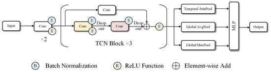
As illustrated in Figure 2, the network is organized into two components: a temporal feature encoding module and a temporal context aggregation and classification module. In the temporal feature encoding module, a 1D convolution layer first performs preliminary feature extraction and cross-channel fusion on the multi-dimensional input sequence. In the subsequent encoding stage, several dilated one-dimensional convolutional residual blocks is stacked to progressively enlarge the temporal receptive field without reducing resolution. This architecture can enable the network to capture both rapid local fluctuations and slower long-range variations within each window.
Figure 2.
Structure of the proposed RA-TCN model.
Based on the high-level features produced by the TCN blocks, the temporal context aggregation module applies self-attentive temporal pooling to adaptively reweight time steps. In parallel, global average and max pooling derive complementary statistics, which are concatenated and fed to a two-layer classifier for binary LOS/NLOS decisions.
3.1. Feature Construction
In this subsection, time-series input features for temporal modeling are constructed from the DS-TWR measurements and PDOA signals collected by the UWB anchor. Let denote the discrete time index. The range and PDOA measurements between the tag and the anchor at time t are denoted by
where is the DS-TWR range estimate, and is the wrapped PDOA measurement (degrees). For trigonometric operations, is converted into radians as
- (1)
- TWR information
Under LOS conditions, the single-anchor range sequence typically evolves smoothly over time, whereas under NLOS conditions, it is prone to gradual drifts, abrupt excursions, and even extended intervals of saturated range estimates. Consequently, we adopt the raw single-anchor range measurements as the primary input signal, without additional smoothing or resampling. The length-T range sequence is denoted as
which serves as the main input of the network.
- (2)
- Angle representation
To fully exploit the single-anchor AOA measurements, the AOA sequence is first computed from the phase differences and then encoded on the unit circle with sine and cosine to remove discontinuity at ±180°. Specifically, at each time step t, we construct a two-dimensional angular feature
Compared with representing the angle as a single scalar, the pair remains continuous when the angle wraps across ±180°. This representation avoids angular discontinuities and facilitates temporal modeling with neural networks. This feature describes the slow evolution of the tag–anchor geometric relationship over time and provides rich information on azimuth differences between LOS and NLOS states.
3.2. Convolutional Neural Network
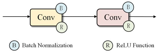
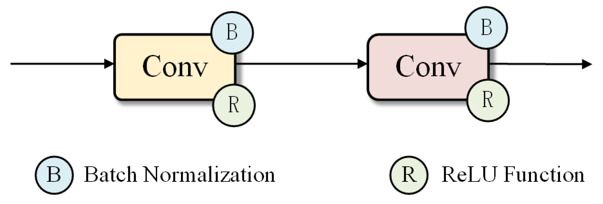
Given a multidimensional time series of length T and feature dimension r, we first transpose it along the temporal and channel dimensions to obtain . The CNN block adopts a one-dimensional convolutional module as the front-end feature extractor, which models the local correlations between adjacent time steps in the range–AOA time series and performs an initial fusion of multi-channel features. Specifically, a one-dimensional convolution is first applied to linearly combine channels and perform information fusion across them. This is followed by a one-dimensional convolution, batch normalization, and a rectified linear unit (ReLU) activation to extract richer local temporal patterns. The overall structure of the convolutional feature extraction block is illustrated in Figure 3.
Figure 3.
Structure diagram of the convolutional feature extraction block in the RA-TCN model.
Through the CNN block, the network can effectively capture short-term nonlinear variations over a limited time window while maintaining a low number of parameters, thereby providing stable and expressive feature representations for subsequent high-level temporal modeling.
3.3. TCN Block
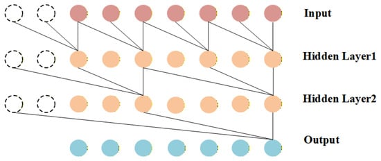
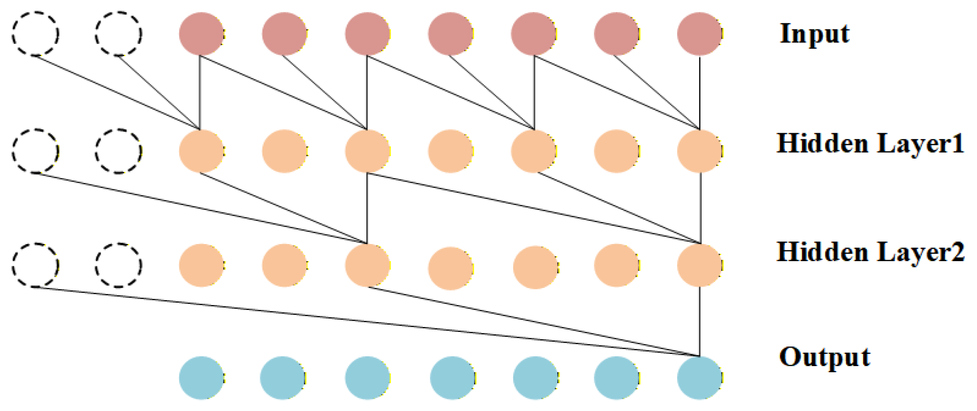
The TCN is a class of convolutional neural networks designed for time-series modeling [30]. Unlike traditional recurrent neural networks (RNNs), TCNs stack multiple one-dimensional convolutions and residual blocks to jointly model long-term and short-term dependencies over an extended temporal window. Compared with standard convolutional architectures, TCNs maintain strong modeling capability with a relatively low computational cost, making them suitable for tasks that analyze multi-step time series within a fixed-length observation window. The core operation in a TCN is the one-dimensional dilated convolution. By inserting gaps between neighboring convolutional elements, dilated convolutions enlarge the receptive field of the kernel without increasing the number of parameters. For an input sequence and a discrete kernel with dilation factor d, the output of a one-dimensional dilated causal convolution at sequence index s is
where ∗ denotes the one-dimensional dilated convolution, s is the sequence index, and k is the kernel size.
As illustrated in Figure 4, by gradually increasing the dilation factor in deeper convolutional layers (e.g., ), the receptive field of the network grows exponentially. Consequently, the TCN can simultaneously capture both fast local fluctuations and slower temporal variations within a relatively short observation window, thereby providing a more comprehensive characterization of temporal patterns.
Figure 4.
Structure diagram of a dilated causal convolution network.
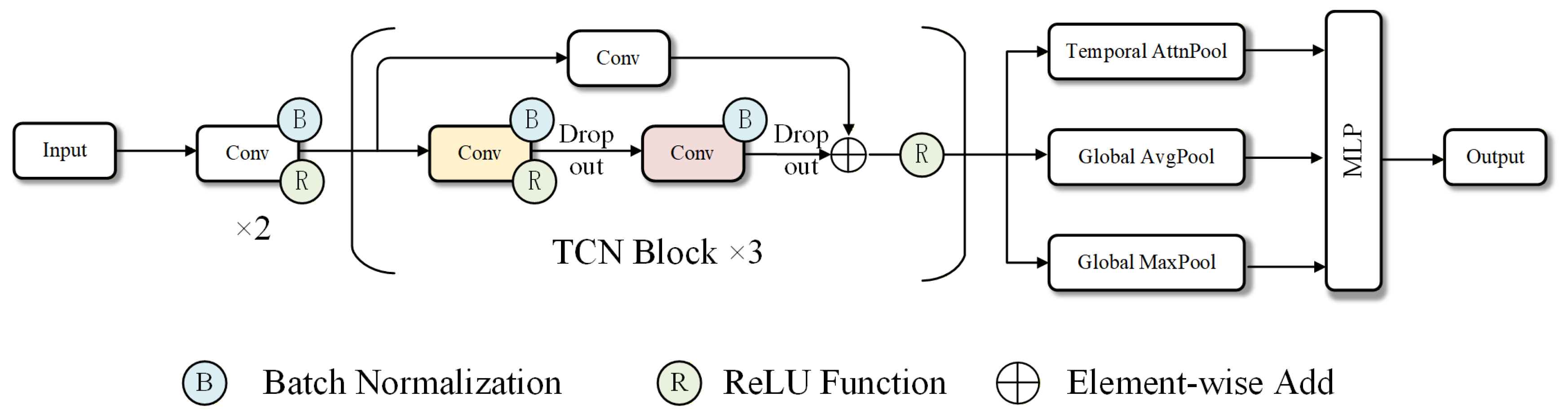
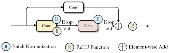
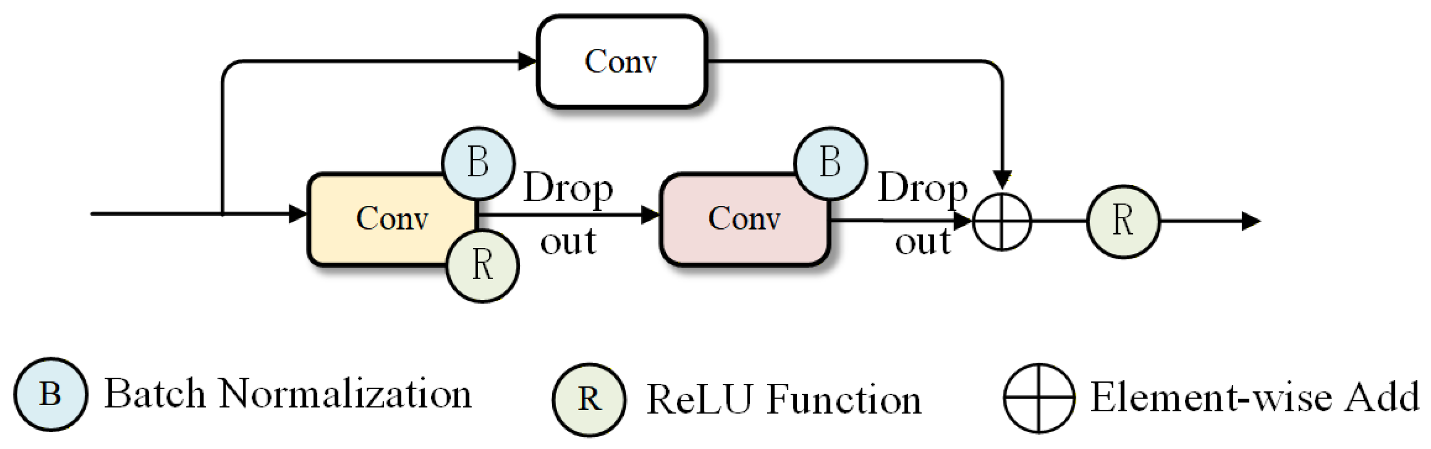
As illustrated in Figure 5, the TCN backbone is constructed by stacking multiple dilated convolutional residual blocks. Each residual block consists of two one-dimensional convolutional layers with kernel size 3, each followed by batch normalization, a ReLU activation, and a dropout layer to enhance the generalization capability of the network. In parallel with the convolutional branch, a residual shortcut connection is introduced; when the number of channels changes, a convolution is applied on the shortcut to match the feature dimensions. The output of the block is obtained by element-wise summation of the shortcut features and the convolutional features, followed by a non-linear activation.
Figure 5.
Structure diagram of a dilated convolutional residual block in the TCN backbone.
3.4. Temporal Attention Module and Classification Module
After being processed by the TCN blocks, the high-level temporal representation of a single-anchor sequence is denoted as , where C is the feature dimension and T is the window length. The model employs a temporal self-attention pooling module to adaptively emphasize time steps that are most informative for classification. This module is combined with global statistical pooling to construct the final classification head.
First, the feature map is transposed along the temporal dimension, , and an attention score is computed for each time step t. Let denote the t-th row of . The attention weights are obtained as
where , , and are learnable parameters, and is the normalized importance weight of the t-th time step. Based on these weights, an attention-based aggregated representation is computed by a weighted sum over all time steps:
To retain complementary global statistical information, global average pooling and global max pooling are further applied to along the temporal dimension, yielding and , respectively. Finally, the three pooled features are concatenated along the channel dimension to form the overall feature vector.
which is fed into a two-layer fully connected network to produce the final classification logits, followed by a softmax layer to obtain class probabilities.
The temporal self-attention mechanism allows the model to learn the relative importance of different time steps within the observation window. The resulting representation concentrates on segments that are most indicative of the underlying propagation state. Meanwhile, the two forms of global statistical pooling provide complementary insights into overall trends and extreme behavior. As a result, the proposed classification module enhances the discriminative power of temporal sequence classification while keeping the total number of parameters relatively small.
3.5. Loss Function Design and Training Strategy
During training, the binary classifier is optimized using a class-weighted cross-entropy loss. Let denote the ground-truth label of the i-th sample and the predicted probability of class k for this sample. The overall loss is defined as
where N is the total number of training samples, and is the normalization coefficient associated with class k. In practice, the class weights are constructed according to the class frequencies in the training set as
To realize adaptive discrimination between LOS and NLOS scenarios, the end-to-end parameters of the temporal convolutional network are optimized using the Adam with decoupled weight decay (AdamW) optimizer with mini-batch training. The initial learning rate is set as , the weight decay coefficient is , and the batch size is fixed to 128. The maximum number of training epochs is set to 50, and an early-stopping strategy based on validation performance is adopted to prevent overfitting. To mitigate stochastic variation in model optimization, all experiments are initialized with fixed random seeds and repeated several times.
The overall network structure of the single-anchor RA-TCN used in this work is summarized in Table 1. During the training, the network parameters are optimized using the AdamW algorithm with a mini-batch size of 128, an initial learning rate of , and a maximum of 50 epochs. In addition, regularization with a weight decay coefficient of and a ReduceLROnPlateau learning-rate scheduling strategy are employed to further improve convergence stability and generalization performance. The proposed RA-TCN-based LOS/NLOS identification framework is presented in pseudocode and summarized in Algorithm 1.
Table 1.
The network structure of the proposed RA-TCN model.
| Algorithm 1 Measurement-driven single-anchor LOS/NLOS identification using RA-TCN. | |
| Require: Raw time series per file ; window length T; stride S; file-level split; RA-TCN ; AdamW; class-weighted cross-entropy; ; max epochs E. | |
| Ensure: Trained parameters . | |
| 1: Split files into . | ▹ File-level split |
| 2: . | ▹ Buffer initialization |
| 3: for each file in do | |
| 4: for do | |
| 5: | |
| 6: | |
| 7: | |
| 8: end for | |
| 9: | ▹ Windowing |
| 10: | ▹ Window labels |
| 11: end for | |
| 12: | ▹ Normalization stats |
| 13: | ▹ Normalize all splits |
| 14: Initialize ; set . | ▹ Model initialization |
| 15: for epoch do | |
| 16: for mini-batch from do | |
| 17: | ▹ Forward |
| 18: | ▹ Loss |
| 19: | ▹ Update |
| 20: end for | |
| 21: Evaluate on ; update ; apply early stopping. | ▹ Model selection |
| 22: end for | |
| 23: Test and report metrics on using . | ▹ Final evaluation |
4. Data Collection and Analysis
4.1. UWB Module
In this paper, the STM32F103RCT6 microcontroller from STMicroelectronics is adopted as the main system controller. It integrates multiple serial peripheral interface (SPI), universal asynchronous receiver/transmitter (UART), and inter-integrated circuit (I2C) interfaces, as well as timer and external-interrupt resources, facilitating real-time control of the UWB transceiver and time-stamp acquisition. The UWB front-end employs Qorvo’s DW3000 series transceiver, released in 2020, which supports IEEE 802.15.4a [31] and IEEE 802.15.4z [32] high-rate pulse UWB. Compared with the previous-generation DW1000, the DW3000 supports IEEE 802.15.4z scrambled timestamp sequence secure sessions and, when combined with dual-antenna variants such as the DW3120/DW3220, provides PDOA-based angle measurement capability [33]. The key configuration parameters of the DWM3000 module used in the experiments are summarized in Table 2.
Table 2.
Configuration parameters of the DWM3000 module in the experiments.
The DW3000 family supports UWB channels 5 and 9, physical data rates of 850 kbps, and 6.8 Mbps, and multiple transmission and reception slot formats. The chip interfaces with the microcontroller unit (MCU) via SPI and exposes register access to key information, such as time stamps and channel impulse responses. According to the DW3000 evaluation module reference design and the official datasheet, after a 10 cm calibration, the typical ranging error of a standard DW3000 under multipath conditions is on the order of 10 cm. For the ranging scenarios considered in this work, the DW3000 also natively supports PDOA with an angular accuracy of approximately . In contrast, the DW1000 requires additional external RF circuitry to achieve a comparable level of angular accuracy.
The single-chip IC with two antenna outputs is well-suited for bi-directional ranging applications with multiple receive channels. It simplifies RF design for dual-antenna PDOA estimation, reduces the overall bill of materials, and eases the layout of dual-antenna structures. At the same time, eliminating additional timing error sources in the external RF front-end contributes to further improvements in ranging accuracy.
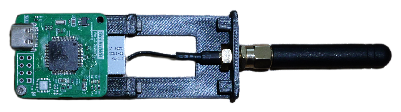
The custom UWB data-acquisition board used in our experiments is shown in Figure 6. The board integrates a Decawave DW3000 transceiver, the matching RF front-end, an MCU interface connector, and a removable UWB antenna. It can be configured as an anchor or a tag and provides time-of-flight ranging and PDOA measurements for the single-anchor LOS/NLOS identification experiments in this work. It should be noted that all measurements in this study were collected using a single DW3000-based module with a fixed chipset and a fixed dual antenna geometry, so generalization across different UWB devices is not assessed here. The temporal cues exploited by RA-TCN, including NLOS-induced positive range bias and increased within-window variability, are primarily determined by propagation mechanisms and are expected to remain qualitatively consistent for UWB platforms that provide comparable DS-TWR ranging and PDOA measurements. Nonetheless, quantitative performance may vary with device-specific factors such as timestamp resolution, internal filtering, RF front-end delays, and calibration, as well as antenna baseline and orientation, which influence the PDOA-to-AOA behavior under multipath.
Figure 6.
DW3000-based UWB board.
4.2. Ranging and AOA Data Collection
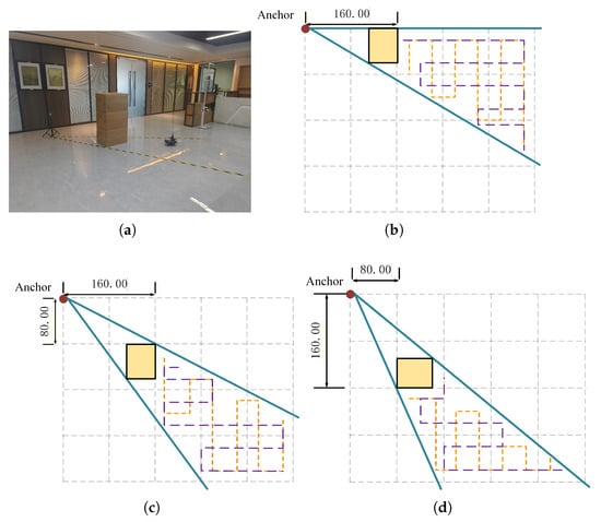
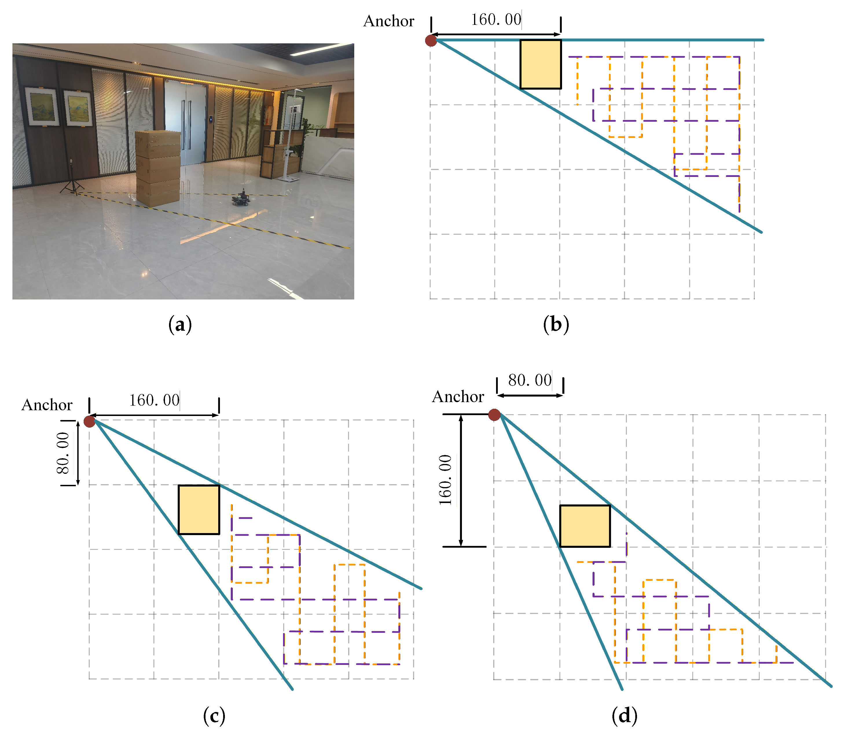
In the experiments, UWB TWR-based range and AOA measurements are acquired in an open-plan office building (Figure 7) using a DWM3000 transceiver from Decawave, Dublin, Ireland. The UWB anchor module is mounted on a tripod at approximately , and a second UWB module is rigidly attached to a small mobile cart at approximately , serving as the moving tag equipped with an inertial sensing unit. In the central region of the test area, obstacle with dimensions are stacked and filled with foam to form a compact obstacle block, thereby defining the NLOS region and blocking direct propagation paths between the anchor and the tag.
Figure 7.
Experimental indoor UWB deployment scenes. (a) Photograph of the experimental environment. (b) Floor plan of Scene 1. (c) Floor plan of Scene 2. (d) Floor plan of Scene 3. Panels (b–d) show the three obstacle layouts. The yellow rectangle denotes the obstacle. The region between the two blue lines indicates the NLOS area. The dashed lines indicate two typical trajectories.
To enrich dataset diversity, three obstacle layouts are configured in the same test area by rearranging the obstacle block. In each layout, the cart is driven within the test area following representative motion patterns, including forward/backward motion, in-place rotations, and high-curvature turns. During motion, the UWB system continuously records single-anchor TWR distances and angles of arrival, forming time-series samples that jointly encode distance and directional information. For each layout, data collection is performed in two stages: In the first stage, the obstacle block is deployed to create NLOS regions. In the second stage, all obstacles are removed while the cart is driven with comparable spatial coverage and maneuvers to collect LOS data. This design encourages the network to learn propagation-dependent characteristics rather than memorizing a specific geometric path.
4.3. Data Analysis
4.3.1. Static Data
To investigate whether temporal variations in the UWB range and phase differences differ under different channel visibility conditions, data are first collected in static scenarios to avoid the influence of target motion on the measurement statistics. If the key fluctuation characteristics of LOS and NLOS are almost identical, then it would be difficult to construct an effective LOS/NLOS classifier based solely on these quantities.
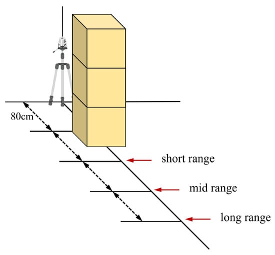
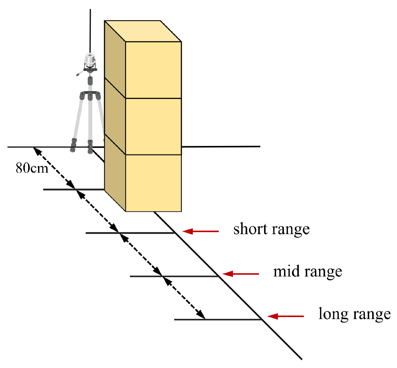
As illustrated in Figure 8, three geometric distance levels (short range, middle range, and long range) were selected, and for each distance, both LOS and NLOS scenarios were constructed, resulting in six operating conditions in total. In LOS cases, there was no obstruction between the anchor and the cart. In NLOS cases, cardboard boxes or walls were placed along the LOS to block the direct line of sight. For each condition, the system continuously recorded the range and phase difference over time, and the statistical properties of their temporal fluctuations were analyzed.
Figure 8.
Experimental setup for static measurement data collection.
For each operating condition, 400 consecutive samples were used as static fluctuation data. To characterize temporal variability, three indicators were employed: the standard deviation of the range , the range span , and the standard deviation of the phase difference . Let the static sequence be denoted as , where is the wrapped PDOA in degrees; then
In LOS scenarios, takes values of 1.76, 2.83, and 2.07 for short, medium, and long distances, respectively, and is 11, 16, and 16. The corresponding range sequences exhibit only small fluctuations around a central value. The phase standard deviations are 7.37, 8.23, and 10.52. In contrast, when moving to NLOS scenarios, increases to 9.43, 46.40, and 31.41, and to 139, 170, and 195. This demonstrates that the range sequences now cover a much wider range and contain frequent abrupt changes and pronounced range biases. Similarly, the phase standard deviations reach 12.19, 19.55, and 60.44, and the phase difference exhibits pronounced excursions in the long-distance case.
Taken together, these indicators show that, for identical distance and gain settings, NLOS links exhibit larger fluctuations in range and phase difference than LOS links. This contrast becomes especially evident at medium and long ranges. As summarized in Table 3, even under static conditions, the temporal fluctuation patterns of TWR and AOA already provide useful statistical features for subsequent data-driven LOS/NLOS classification.
Table 3.
Performance comparison of LOS/NLOS statistics at different ranges.
4.3.2. Dynamic Data
This subsection compares UWB ranging under LOS and NLOS by analyzing two motion segments. To investigate whether temporal variations in the UWB range and PDOA measurements differ under different channel visibility conditions, where P is wrapped to .
The time series is segmented into overlapping sliding windows of length with a stride of 30. For each window, the following statistics are computed:
- 1.
- The standard deviation and range of the distance sequence.
- 2.
- The standard deviation of the first-order difference of the distance sequence, denoted by .
- 3.
- The standard deviation of the phase-difference sequence and the standard deviation of its first-order difference .
As shown in Table 4, for each metric the table reports the mean and standard deviation across all windows for both LOS and NLOS conditions. Range fluctuations under NLOS are substantially stronger than under LOS. For example, the mean increases from (LOS) to (NLOS), and the mean within-window range increases from to (in the device’s native ranging units).
Table 4.
Statistical comparison of dynamic range and angle features under LOS and NLOS conditions.
The first-order difference shows a consistent trend: the mean increases from (LOS) to (NLOS), indicating that once the direct path is obstructed, the TWR-based range estimates exhibit more frequent abrupt variations.
Phase-difference-related features also exhibit clear separability. The mean increases from (LOS) to (NLOS), and the mean rises from to . These increases reflect intensified temporal instability of the measured PDOA under NLOS propagation.
5. Experiments and Analysis
5.1. Experimental Settings and Dataset Description
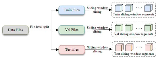
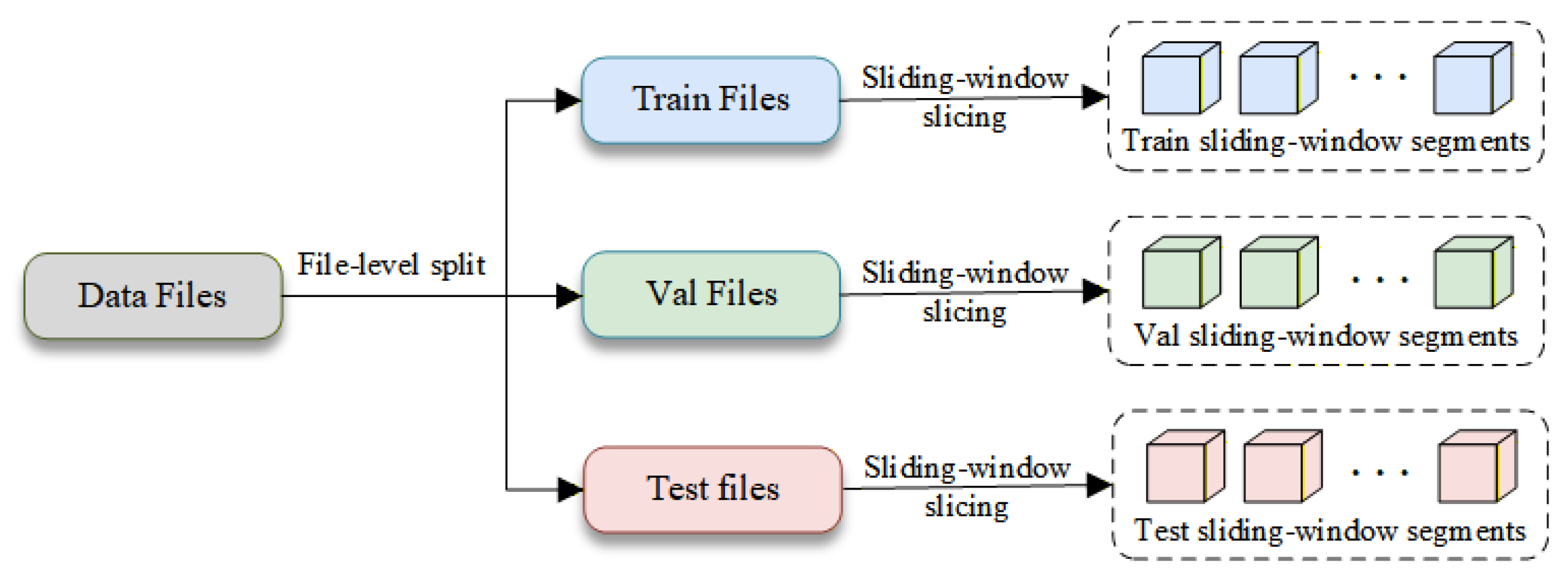
A time-series dataset is constructed from the collected single-anchor UWB TWR-based range and AOA measurements to support LOS/NLOS identification. The dataset contains in a total of valid samples, of which are LOS and are NLOS. All measurements are obtained using a single-antenna transmission mode with an inter-ranging delay of 200 ms in an indoor office with fixed obstacles. As shown in Figure 9, the dataset is split at the file level into training where files are randomly assigned to each subset to avoid temporal overlap. During training, sliding windows of length and stride 50 are used to segment the time series. In the validation and test phases, the window length is set to , and non-overlapping windows (stride T) are used to ensure statistical independence between windows.
Figure 9.
Dataset split flowchart.
All experiments are conducted on a Windows 11 computing platform equipped with a 13th Gen Intel® Core™ i7-13650HX CPU, Intel, Corporation, Santa Clara, CA, USA; an NVIDIA RTX 4060 GPU, NVIDIA Corporation, Santa Clara, CA, USA; and 32 GB of RAM. The proposed RA-TCN model is implemented using the PyTorch v2.2.2 framework. In addition, to reflect real-time feasibility in IoT settings, the computational cost of RA-TCN is profiled under the above implementation. RA-TCN contains 7.65k parameters and requires 0.704 MFLOPs per window.
The performance of the proposed single-anchor RA-TCN model on the LOS/NLOS classification task is evaluated using accuracy, recall, precision, and the F1-score. In all experiments, NLOS samples are treated as the positive class and LOS samples as the negative class. Let , , , and denote the numbers of true positives, true negatives, false positives, and false negatives, respectively. The classification accuracy is defined as
To further characterize the detection capability of the model for the NLOS state, recall, precision, and F1-score are defined as
Recall is the proportion of NLOS samples correctly identified among all NLOS samples, precision is the reliability of the model’s NLOS predictions, and the F1-score is the harmonic mean of precision and recall, providing a comprehensive and balanced indicator of classification performance.
5.2. Comparative Experiments with Different Models
In this subsection, the proposed single-anchor RA-TCN is evaluated against several representative deep learning models. These include a CNN–LSTM model [34], a CNN with a multilayer perceptron classifier (MLP) (CNN–MLP) [35], the 1D channel-attention network (CLA) [36], an attention-based deep CNN–BiLSTM (ADCNN–BiLSTM) model [37] and a support vector machine (SVM) [26]. All models are trained and evaluated on the merged Scene 1–3 dataset using file-level splits within each scene to prevent leakage. The CNN-LSTM model adopts a stacked architecture composed of a one-dimensional CNN followed by two BiLSTM layers. The remaining baselines follow the architectural settings described in their original papers.
All deep learning baselines were designed for CIR inputs and are re-implemented on the same TWR+angle features as the proposed model, so the comparison mainly reflects differences in network architectures under identical inputs. All models are retrained on our dataset with the same splits and optimization settings as the proposed method.
All methods in Table 5 are trained and evaluated on exactly the same single-anchor time-series dataset, with identical window segmentation, feature construction, and preprocessing. The only difference between the methods lies in the choice of network architecture. As shown in Table 5, When compared specifically against the neural-network baselines, RA-TCN consistently delivers the highest recall and F1-score, indicating a stronger capability to identify NLOS samples while maintaining high precision. In particular, relative to the weakest deep learning baseline (CNN–LSTM), RA-TCN improves accuracy, precision, recall, and F1-score by 6.64, 6.87, 6.01, and 6.93 percentage points, respectively. Moreover, RA-TCN still provides consistent gains over the stronger CLA and ADCNN baselines, especially in recall and F1-score, indicating an enhanced ability to detect NLOS samples without sacrificing overall classification performance.
Table 5.
Performance comparison of various approaches for NLOS binary classification.
The CNN-LSTM and CLA families rely on one-dimensional convolutional layers, which are optionally combined with channel-attention mechanisms, to extract local temporal patterns and salient channels. Their convolution-dominated designs are effective at capturing short-range dependencies but are less suited to modeling longer-term and non-stationary temporal dynamics. Consequently, their recall and F1-score remain lower than those of the proposed multi-layer TCN with global attention pooling, which explicitly enlarges the receptive field through dilated convolutions and leverages attention to emphasize informative time steps.
The CNN–MLP baseline first employs CNN blocks to extract intermediate temporal features, then aggregates them through fully connected layers. While this structure balances complexity and accuracy, its limited representational power results in performance between CNN-LSTM and CLA, as shown in our experiments.
The deep learning-based ADCNN–BiLSTM model combines convolutional layers, bidirectional LSTM units, and attention-enhanced temporal features and has demonstrated strong performance in previous LOS/NLOS studies. However, its architecture is considerably more complex, with a large number of parameters. Given the relatively modest data scale and reduced feature dimensionality considered here, this model tends to suffer from mild overfitting, resulting in slightly lower overall performance than the more compact RA-TCN.
In addition to deep models, SVM is included as a classical non-neural baseline. As reported in Table 5, SVM yields an accuracy of and a F1-score of , which is notably lower than all deep learning approaches. This gap is expected because SVM operates on a fixed feature representation and does not explicitly model multi-scale temporal dependencies within the window. In contrast, RA-TCN learns hierarchical temporal patterns through dilated convolutions and further emphasizes discriminative time steps via attention pooling, which is particularly beneficial for capturing sustained NLOS bias and non-stationary fluctuations in range and AOA sequences.
Taken together, these results show that the proposed RA-TCN benefits from jointly modeling the single-anchor range sequence and the sine–cosine encoded AOA sequence within a temporal convolutional and attention pooling framework.
5.3. Cross-Scene Generalization Test
Cross-scene generalization is evaluated using a leave-one-scene-out protocol. Each scene corresponds to a distinct obstacle placement in the same indoor site (Figure 7). One scene is held out as an unseen test environment in each evaluation fold.
This protocol is adopted to quantify robustness under layout-induced distribution shift. It prevents training and testing on samples collected under the same obstacle configuration. It also matches practical deployment where the obstacle layout may change after training. In each fold, all files from the held-out scene are reserved for testing. Files from the two training scenes are split at the file level into training and validation subsets. The validation subset is used for early stopping and model selection. Window segmentation follows Section 3.1 with . The evaluation follows the same preprocessing and training protocol as in the preceding comparative experiments. Table 6 reports the classification accuracy obtained on the held-out scene for each split.
Table 6.
Cross scene generalization accuracy (%) under a held out scene evaluation.
Table 6 summarizes the results under scene hold-out evaluation. RA-TCN yields the highest accuracy for each held-out scene. The strongest baseline achieves 91.62%, 86.03%, and 87.70% on all test Scenes, respectively. RA-TCN exceeds these values by 1.94, 2.69, and 2.71 percentage points. All methods obtain the lowest accuracy when Scene 2 is used as the test scene. RA-TCN varies from 88.72% to 93.56% across splits, indicating stable transfer under layout changes. These results align with the multi-scale temporal modeling and attention pooling described in Section 3.
5.4. Test Experiments for Robustness to Different Window Sizes
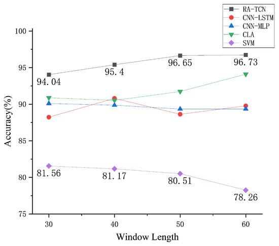
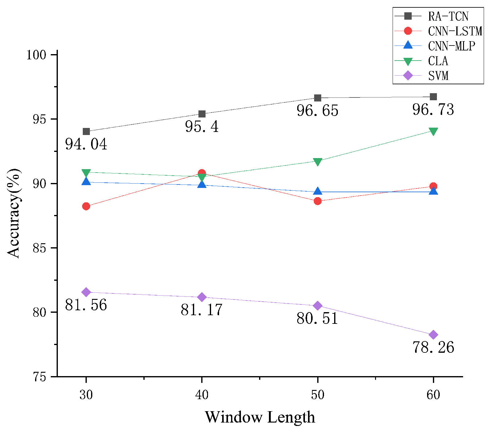
The robustness of the proposed model to the temporal scale is further assessed by examining its classification performance under different segment window lengths. All experiments are conducted on the same single-anchor TWR and AOA dataset, and experimental configuration described in Section 4, and only the length of the sliding window used to segment the range–angle sequences is varied. Specifically, the window length T is set to 30, 40, 50, and 60 time steps, and the classification accuracies of the proposed method and five baseline models (CNN–LSTM, CNN–MLP, CLA, ADCNN–BiLSTM and SVM) are compared.
As shown in Figure 10, the proposed RA-TCN consistently achieves the highest accuracy across all window lengths. With larger T, the accuracy increases from at to at , and remains nearly unchanged at . This indicates that extending the temporal context helps the network better capture the temporal patterns associated with LOS/NLOS transitions, while the performance gain becomes marginal beyond a moderate window length. In comparison, the baseline methods show lower accuracies and more model-dependent sensitivity to the window size. CNN–LSTM fluctuates with T rather than monotonically improving. CLA and ADCNN benefit more evidently from longer windows and achieve higher accuracies at , yet they still lag behind RA-TCN. In addition, SVM yields the lowest accuracy overall and even degrades as T increases, suggesting limited ability to exploit longer temporal contexts under a fixed feature representation. Overall, these results demonstrate that RA-TCN can effectively exploit longer temporal contexts and deliver more stable LOS/NLOS identification performance across different window-length configurations than the CNN–LSTM, CNN–MLP, CLA, ADCNN and SVM baselines.
Figure 10.
Comparison of LOS/NLOS classification accuracy of different models under varying temporal window lengths.
Based on these observations, is selected as the default window length. RA-TCN reaches near-saturated accuracy at , and the gain from is marginal. Longer windows also reduce the number of training segments under the same protocol. For CLA model, the accuracy increases when T increases from 40 to 50. This suggests that a longer window does not always improve performance. It also indicates that the optimal window length is model-dependent. They are more likely to cover LOS/NLOS transitions, which can increase label ambiguity. Therefore, provides a robust trade-off for subsequent experiments.
5.5. Ablation Experiments
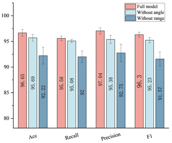
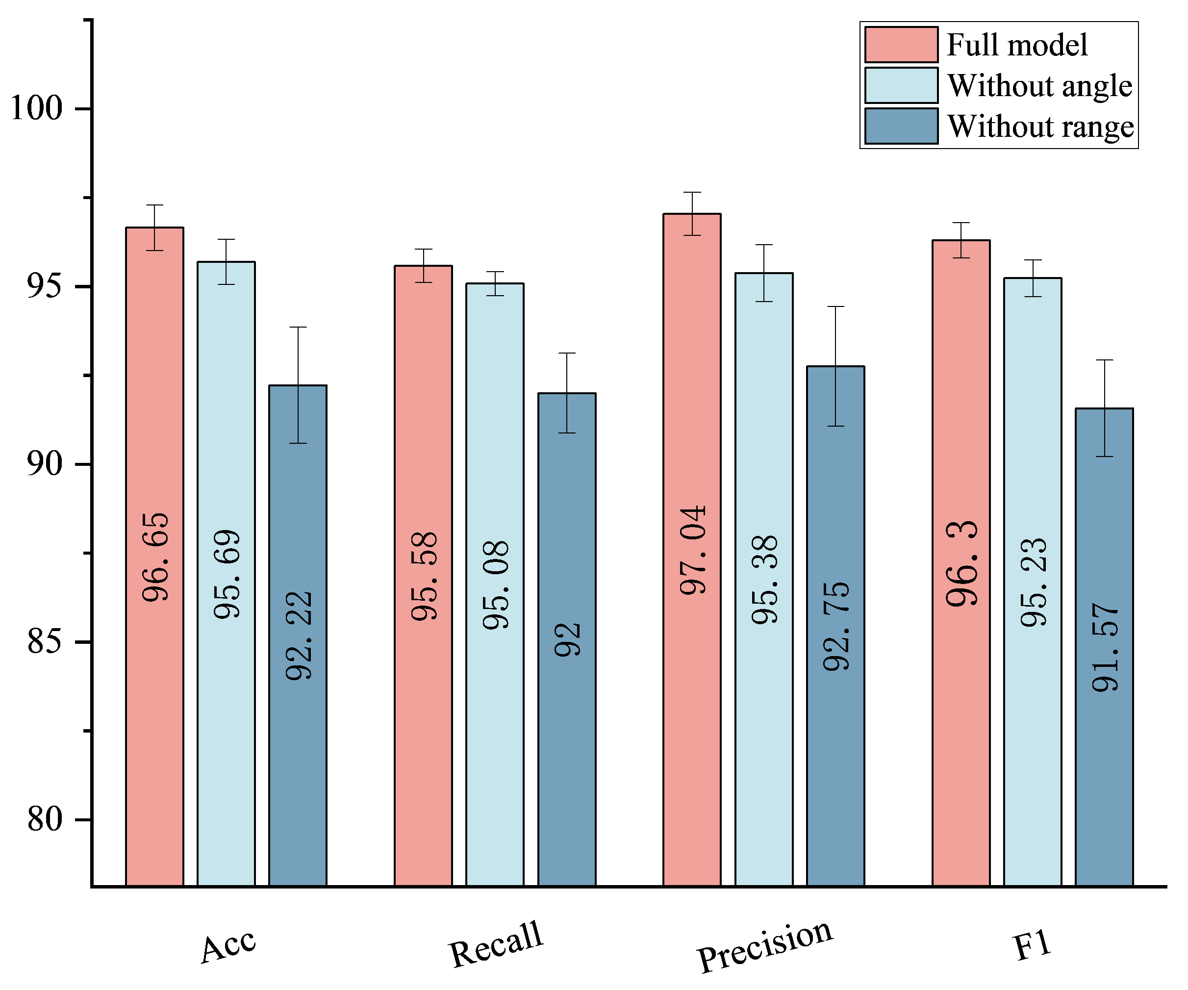
In the full configuration, the input representation consists of the range sequence and a sine–cosine encoded AOA sequence, i.e., . Two ablation settings are further considered: range-only () and angle-only (). Under this setting, the accuracy reaches , and the macro-averaged precision, recall, and F1-score are , , and spectively, indicating balanced and robust discrimination between LOS and NLOS conditions.
Figure 11 reports the ablation results in terms of mean performance and standard deviation over five independent runs. When angle-domain components are removed, and only the range sequence is retained, the accuracy drops to and the F1 decreases to . In contrast, discarding range measurements and keeping only angular cues causes a larger degradation, with an accuracy of and a F1 of . These results indicate that range provides the dominant constraint, while angle offers a limited but consistent gain. The angle cue is less stable under multipath. The mean within-window phase standard deviation increases from degrees in LOS to degrees in NLOS. The mean standard deviation of phase differences increases from degrees to degrees. The transceiver does not provide a standardized per-sample AOA confidence, and AOA quality varies with calibration, hardware bias, and multipath. Therefore, explicit confidence weighting is not adopted, and attention pooling suppresses unstable time steps. The limited fusion gain may also relate to motion-induced heading changes that perturb AOA beyond propagation effects.
Figure 11.
Comparative results of input ablation in RA-TCN.
Notably, a naive confidence weighting based on instantaneous AOA variation can be unreliable in our setting, because the observed angle dynamics are jointly influenced by propagation and motion. Rapid maneuvers can induce genuine AOA changes even under LOS, while some NLOS links may exhibit a stable apparent direction when a dominant reflected path persists. In such cases, heuristic weights may suppress informative segments. Instead, self-attentive pooling performs data-driven temporal reweighting conditioned on the joint range angle context, serving as an implicit reliability selection without requiring per-sample confidence. Future work will incorporate motion sensing and uncertainty modeling to enable more principled confidence weighting.
5.6. Discussion
The comparative results in Table 5 show that RA-TCN reaches accuracy and a macro F1-score of on the merged dataset. Under leave-one-scene-out evaluation in Table 6, it maintains accuracies between and across held-out scenes. The performance gain is consistent with the temporal design of the model. Dilated residual convolutions capture multi-scale temporal patterns within a fixed window. Self-attentive pooling highlights informative time segments and is more effective when NLOS cues appear only in part of the window. The ablation results in Figure 11 also indicate that range and angle cues are complementary. DS-TWR range provides the primary discriminative signal, while PDOA-derived AOA offers auxiliary evidence.
An inspection of misclassified windows suggests two dominant error sources. One source arises when NLOS segments are predicted as LOS, which is more likely under mild blockage or partial obstruction. In such cases, a residual direct component may remain, leading to a small ranging bias and temporal fluctuation statistics that approach those of LOS. The PDOA-derived angular cue may also contribute limited evidence, because multipath can yield a relatively stable apparent direction, and the sine–cosine representation varies only slightly within the window. In addition, NLOS is not necessarily characterized by abrupt spikes. When the tag is sufficiently far from obstacles, a stable reflected or diffracted component may dominate, producing a quasi-stationary positive offset in the range sequence while leaving the short-term variance nearly unchanged. These overall-shift patterns are therefore more easily confused with LOS.
Another source corresponds to LOS segments that are predicted as NLOS. Even without physical obstruction, rich multipath information can induce intermittent ranging spikes, and rapid maneuvers may trigger changes in the dominant propagation component. Occasional timestamp irregularities can further introduce outliers. Collectively, these factors increase within-window variability and may resemble NLOS-like temporal instability. Angle-related confusion is further influenced by inherent limitations of PDOA-based AOA, including front–back ambiguity and multipath-dominant arrivals that distort the apparent bearing. Rapid switching of the dominant path can also yield irregular angular trajectories, which may be interpreted as NLOS-like behavior. Finally, a persistent systematic offset in the range measurements, for example, due to calibration drift or hardware bias, can resemble the overall-shift signature and increase the likelihood of false alarms when it aligns with learned NLOS patterns.
6. Conclusions
This paper investigated LOS/NLOS identification for single-anchor UWB indoor localization using time-series TWR range- and PDOA-derived AOA measurements, without relying on raw CIR access. A measurement-driven RA-TCN was developed by combining a convolutional front-end, dilated TCN residual blocks, and self-attentive temporal pooling. Experiments on the collected dataset indicate that the RA-TCN consistently outperforms the compared deep learning baselines, achieving an identification accuracy of 96.65%, with a precision of 97.04% and a recall of 95.58%. Additional analyses suggest that temporal aggregation and multi-scale modeling are key to exploiting range–angle dynamics and that range and angle cues provide complementary information under different window lengths. Overall, the proposed design is deployable on commodity devices and is suitable for infrastructure-constrained single-anchor scenarios. Nevertheless, the performance gain from range–angle fusion remains modest, and the current evaluation is constrained by site-specific conditions. In particular, evidence is drawn from a single indoor site with a limited number of obstacle layouts, and the absence of reliable ground-truth trajectories prevents trajectory-aware supervision and more realistic protocol design.
Future work will investigate more expressive fusion mechanisms and extend measurement campaigns to multiple sites and richer obstacle configurations. Specifically, the proposed RA-TCN can be applied to each anchor–tag link independently to output an NLOS posterior probability, which can be used as a reliability weight for measurement screening or weighted fusion in subsequent ToF-based localization, enabling straightforward scaling from single-anchor to multi-anchor deployments. In addition, multi-device UWB fusion and auxiliary sensing will be explored to improve robustness under motion and intermittent blockage. The LOS/NLOS outputs will be incorporated into ToF-based positioning pipelines to quantify end-to-end localization gains and to enable mitigation beyond identification.
Author Contributions
Conceptualization, Y.Z. (Yuhao Zeng); methodology, Y.Z. (Yuhao Zeng); validation, D.W.; resources, L.Z.; visualization, Z.L.; writing—original draft preparation, Y.Z. (Yuhao Zeng); writing—review and editing, Y.Z. (Yuhao Zeng) and D.Z.; supervision, G.Y. and Y.Z. (Yuhong Zhang); data curation, Y.Z. (Yuhao Zeng) and S.Z. All authors have read and agreed to the published version of the manuscript.
Funding
This research was funded by Shenzhen Science and Technology Program (Grant No. KCXFZ20240903094011015).
Data Availability Statement
The datasets that support the findings of this study are available on request from the corresponding author, upon reasonable request.
Acknowledgments
The authors would like to thank the editors and reviewers for their detailed reviews and suggestions on the manuscript.
Conflicts of Interest
The authors declare no conflicts of interest.
Abbreviations
The following abbreviations are used in this manuscript:
| IoT | Internet of Things |
| UWB | Ultra-Wideband |
| NLOS | Non-Line-of-Sight |
| LOS | Line-of-Sight |
| TWR | Two-Way Ranging |
| AOA | Angle-of-Arrival |
| TCN | Temporal Convolutional Network |
| IPS | Indoor Positioning Systems |
| CIR | Channel Impulse Response |
| CNN | Convolutional Neural Network |
| LSTM | Long Short-Term Memory |
| BiLSTM | Bidirectional Long Short-Term Memory |
| DS-TWR | Double-Sided Two-Way Ranging |
| PDOA | Phase-Difference-of-Arrival |
| RA-TCN | Ranging-AOA Temporal Convolutional Network |
| ReLU | Rectified Linear Unit |
| RNN | Recurrent Neural Network |
| FC | Fully Connected (layer) |
| AdamW | Adam with Decoupled Weight Decay |
| Regularization | |
| MCU | Microcontroller Unit |
| SPI | Serial Peripheral Interface |
| UART | Universal Asynchronous Receiver/Transmitter |
| I2C | Inter-Integrated Circuit |
| F1 | F1-score |
| TP | True Positive |
| TN | True Negative |
| FP | False Positive |
| FN | False Negative |
| MLP | Multi-Layer Perceptron |
| CLA | Channel-Attention Network |
| ADCNN–BiLSTM | Attention-based Deep CNN with BiLSTM |
References
- Li, C.; Zhen, J.; Chang, K.; Xu, A.; Zhu, H.; Wu, J. An Indoor Positioning and Tracking Algorithm Based on Angle-of-Arrival Using a Dual-Channel Array Antenna. Remote Sens. 2021, 13, 4301. [Google Scholar] [CrossRef] [Scilit]
- Asaad, S.M.; Maghdid, H.S. A comprehensive review of indoor/outdoor localization solutions in IoT era: Research challenges and future perspectives. Comput. Netw. 2022, 212, 109041. [Google Scholar] [CrossRef] [Scilit]
- Leitch, S.G.; Ahmed, Q.Z.; Abbas, W.B.; Hafeez, M.; Laziridis, P.I.; Sureephong, P.; Alade, T. On Indoor Localization Using Wi-Fi, BLE, UWB, and IMU Technologies. Sensors 2023, 23, 8598. [Google Scholar] [CrossRef] [Scilit]
- Dardari, D.; Conti, A.; Ferner, U.; Giorgetti, A.; Win, M.Z. Ranging with Ultrawide Bandwidth Signals in Multipath Environments. Proc. IEEE 2009, 97, 404–426. [Google Scholar] [CrossRef] [Scilit]
- Zafari, F.; Gkelias, A.; Leung, K.K. A Survey of Indoor Localization Systems and Technologies. IEEE Commun. Surv. Tutor. 2019, 21, 2568–2599. [Google Scholar] [CrossRef] [Scilit]
- Tong, X.; Liu, K.; Tian, X.; Fu, L.; Wang, X. FineLoc: A Fine-Grained Self-Calibrating Wireless Indoor Localization System. IEEE Trans. Mob. Comput. 2018, 18, 2077–2090. [Google Scholar] [CrossRef] [Scilit]
- Liu, H.; Yang, J.; Sidhom, S.; Wang, Y.; Chen, Y.; Ye, F. Accurate WiFi-Based Localization for Smartphones Using Peer Assistance. IEEE Trans. Mob. Comput. 2013, 13, 2199–2214. [Google Scholar] [CrossRef] [Scilit]
- Qiao, G.; Muhammad, A.; Muzzammil, M.; Khan, M.S.; Tariq, M.O.; Khan, M.S. Addressing the Directionality Challenge through RSSI-Based Multilateration Technique, to Localize Nodes in Underwater WSNs by Using Magneto-Inductive Communication. J. Mar. Sci. Eng. 2022, 10, 530. [Google Scholar] [CrossRef] [Scilit]
- Cheraghinia, M.; Shahid, A.; Luchie, S.; Gordebeke, G.J.; Caytan, O.; Fontaine, J.; De Poorter, E. A Comprehensive Overview on UWB Radar: Applications, Standards, Signal Processing Techniques, Datasets, Radio Chips, Trends and Future Research Directions. IEEE Commun. Surv. Tutor. 2025, 27, 2283–2324. [Google Scholar] [CrossRef] [Scilit]
- Marano, S.; Gifford, W.M.; Wymeersch, H.; Win, M.Z. NLOS Identification and Mitigation for Localization Based on UWB Experimental Data. IEEE J. Sel. Areas Commun. 2010, 28, 1026–1035. [Google Scholar] [CrossRef] [Scilit]
- Tu, C.; Zhang, J.; Quan, Z.; Ding, Y. UWB Indoor Localization Method Based on Neural Network Multi-Classification for NLOS Distance Correction. Sens. Actuators A Phys. 2024, 379, 115904. [Google Scholar] [CrossRef] [Scilit]
- Park, J.; Nam, S.; Choi, H.; Ko, Y.; Ko, Y.-B. Improving Deep Learning-Based UWB LOS/NLOS Identification with Transfer Learning: An Empirical Approach. Electronics 2020, 9, 1714. [Google Scholar] [CrossRef] [Scilit]
- Ghaemifar, M.; Ebadollahi, S.; Ghasemzadeh, M.; Pirahmadian, S. A Novel CNN Model for NLOS Classification in UWB Indoor Positioning System. In Proceedings of the 2024 10th International Conference on Web Research (ICWR), Tehran, Iran, 24–25 April 2024; IEEE: Piscataway, NJ, USA, 2024; pp. 182–186. [Google Scholar] [CrossRef] [Scilit]
- Cui, Z.; Gao, Y.; Hu, J.; Tian, S.; Cheng, J. LOS/NLOS Identification for Indoor UWB Positioning Based on Morlet Wavelet Transform and Convolutional Neural Networks. IEEE Commun. Lett. 2021, 25, 879–882. [Google Scholar] [CrossRef] [Scilit]
- Wei, J.; Wang, H.; Su, S.; Tang, Y.; Guo, X.; Sun, X. NLOS Identification Using Parallel Deep Learning Model and Time-Frequency Information in UWB-Based Positioning System. Measurement 2022, 195, 111191. [Google Scholar] [CrossRef] [Scilit]
- Deng, B.; Xu, T.; Yan, M. UWB NLOS Identification and Mitigation Based on Gramian Angular Field and Parallel Deep Learning Model. IEEE Sens. J. 2023, 23, 28513–28525. [Google Scholar] [CrossRef] [Scilit]
- Deng, X.; Ping, Z.; Sun, R. UWB NLOS Recognition Based on Improved Convolutional Neural Network Assisted by Wavelet Analysis and Gramian Angular Field. IEEE Sens. J. 2023, 23, 16384–16392. [Google Scholar] [CrossRef] [Scilit]
- Li, Z.; Zheng, W.; Feng, B. Semi-Supervised Algorithm SoftMatch for UWB Channel State Identification Based on Continuous Wavelet Transform and Gramian Angular Field. IEEE Sens. J. 2025, 25, 29111–29123. [Google Scholar] [CrossRef] [Scilit]
- Kim, D.-H.; Farhad, A.; Pyun, J.-Y. UWB Positioning System Based on LSTM Classification with Mitigated NLOS Effects. IEEE Internet Things J. 2022, 10, 1822–1835. [Google Scholar] [CrossRef] [Scilit]
- Yang, H.; Wang, Y.; Seow, C.K.; Sun, M.; Coene, S.; Huang, L.; Joseph, W.; Plets, D. Fuzzy Transformer Machine Learning for UWB NLOS Identification and Ranging Mitigation. IEEE Trans. Instrum. Meas. 2025, 74, 8503817. [Google Scholar] [CrossRef] [Scilit]
- Yang, H.; Wang, Y.; Seow, C.K.; Li, Z.; Sun, M.; De Cock, C.; Bi, J.; Joseph, W.; Plets, D. NLOS Identification and Ranging Trustworthiness for Indoor Positioning with LLM-Based UWB-IMU Fusion. IEEE Trans. Instrum. Meas. 2025, 74, 8509417. [Google Scholar] [CrossRef] [Scilit]
- Zhang, D.; Xu, H.; Zhan, L.; Li, Y.; Yin, G.; Wang, X. Accurate Joint Estimation of Position and Orientation Based on Angle of Arrival and Two-Way Ranging of Ultra-Wideband Technology. Electronics 2025, 14, 429. [Google Scholar] [CrossRef] [Scilit]
- Yang, H.; Wang, Y.; Seow, C.K.; Sun, M.; Si, M.; Huang, L. UWB Sensor-Based Indoor LOS/NLOS Localization with Support Vector Machine Learning. IEEE Sens. J. 2023, 23, 2988–3004. [Google Scholar] [CrossRef] [Scilit]
- Ma, T.; Zhang, D.; Zhuang, J.; You, C.; Yin, G.; Tang, S. TDOA-Based UWB Indoor 1D Localization via Weighted Sliding Window Filtering. Digit. Signal Process. 2024, 151, 104544. [Google Scholar] [CrossRef] [Scilit]
- Kolakowski, M.; Modelski, J. Detection of Direct Path Component Absence in NLOS UWB Channel. In Proceedings of the 2018 22nd International Microwave and Radar Conference (MIKON), Poznan, Poland, 14–17 May 2018; pp. 247–250. [Google Scholar] [CrossRef] [Scilit]
- Huang, C.; Molisch, A.F.; He, R.; Wang, R.; Tang, P.; Ai, B.; Zhong, Z. Machine Learning-Enabled LOS/NLOS Identification for MIMO Systems in Dynamic Environments. IEEE Trans. Wirel. Commun. 2020, 19, 3643–3657. [Google Scholar] [CrossRef] [Scilit]
- Silva, B.J.; Hancke, G.P. Non-Line-of-Sight Identification Without Channel Statistics. In Proceedings of the IECON 2020—46th Annual Conference of the IEEE Industrial Electronics Society, Singapore, 18–21 October 2020; pp. 4489–4493. [Google Scholar] [CrossRef] [Scilit]
- Cheng, L.; Huang, S.; Xue, M.; Bi, Y. A Robust Localization Algorithm Based on NLOS Identification and Classification Filtering for Wireless Sensor Network. Sensors 2020, 20, 6634. [Google Scholar] [CrossRef] [Scilit]
- Zhao, Y.; Zhou, Z.; Zou, J.; Guo, J.; Huang, G.; Wu, J. Ultra-Wideband Ranging Data Reconstruction and Positioning Calculation Framework in Indoor Low-Dynamic Scenarios. IEEE Trans. Instrum. Meas. 2025, 74, 1013017. [Google Scholar] [CrossRef] [Scilit]
- Bai, S.; Kolter, J.Z.; Koltun, V. An Empirical Evaluation of Generic Convolutional and Recurrent Networks for Sequence Modeling. arXiv 2018, arXiv:1803.01271. Available online: https://arxiv.org/abs/1803.01271 (accessed on 2 December 2025).
- IEEE Std 802.15.4a-2007; IEEE Standard for Information Technology—Local and Metropolitan Area Networks—Specific Requirements—Part 15.4: Wireless Medium Access Control (MAC) and Physical Layer (PHY) Specifications for Low-Rate Wireless Personal Area Networks (WPANs): Amendment 1: Add Alternate PHYs. IEEE: New York, NY, USA, 2007.
- IEEE Std 802.15.4z-2020; IEEE Standard for Low-Rate Wireless Networks—Amendment 1: Enhanced Ultra Wideband (UWB) Physical Layers (PHYs) and Associated Ranging Techniques. IEEE: New York, NY, USA, 2020.
- Decawave Ltd. DW3000 Family User Manual: How to Use, Configure and Control the DW3000 UWB Transceiver; Version 1.1; Decawave Ltd.: Dublin, Ireland, 2019; Available online: https://www.qorvo.com/products/d/da008154 (accessed on 5 December 2025).
- Xu, J.; Liu, Y.; Jia, Y.; Guo, G.; Cao, S. Acoustic NLOS Signal Recognition Based on 1-D Convolutional Neural Network with Channel Attention Mechanism. IEEE Trans. Instrum. Meas. 2025, 74, 3522630. [Google Scholar] [CrossRef] [Scilit]
- Si, M.; Wang, Y.; Siljak, H.; Seow, C.; Yang, H. A Lightweight CIR-Based CNN with MLP for NLOS/LOS Identification in a UWB Positioning System. IEEE Commun. Lett. 2023, 27, 1332–1336. [Google Scholar] [CrossRef] [Scilit]
- Wang, Q.; Chen, M.; Liu, J.; Lin, Y.; Li, K.; Yan, X.; Zhang, C. 1D-CLANet: A Novel Network for NLOS Classification in UWB Indoor Positioning System. Appl. Sci. 2024, 14, 7609. [Google Scholar] [CrossRef] [Scilit]
- Qi, L.; Zhao, Y.; Guo, Q.; Kaliuzhnyi, M.; Wang, E. Deep Learning-Based NLOS Identification of UWB Signals. IEEE Signal Process. Lett. 2025, 32, 2394–2398. [Google Scholar] [CrossRef] [Scilit]

Disclaimer/Publisher’s Note: The statements, opinions and data contained in all publications are solely those of the individual author(s) and contributor(s) and not of MDPI and/or the editor(s). MDPI and/or the editor(s) disclaim responsibility for any injury to people or property resulting from any ideas, methods, instructions or products referred to in the content. |
© 2026 by the authors. Licensee MDPI, Basel, Switzerland. This article is an open access article distributed under the terms and conditions of the Creative Commons Attribution (CC BY) license.