Research on Optimization Algorithm of High-Precision Localization Loss Function Based on Boundary Box

Abstract

The design of bounding box loss functions directly impacts the localization performance and overall accuracy of object detection models. Bounding box loss functions constructed based on Intersection over Union (IoU) tend to induce anchor box expansion during the optimization process, and the design of certain penalty factors can impede anchor box regression. To address these issues, this study first conducts an in-depth analysis of the causes of anchor box expansion and the flaws in the design of some penalty factors. It then proposes a method to construct the loss function using diagonal lines as an equivalent substitute for anchor boxes, converting the anchor box regression problem into diagonal regression. Second, a new metric termed “$L_1+L_2$” is introduced, where $L_1$ and $L_2$ denote the Euclidean distances between the corresponding top-left and bottom-right vertices of the predicted and ground-truth boxes, respectively. Based on this metric, the Two-Point Loss (TPL) is constructed. This loss function can accurately measure the geometric differences between anchor boxes while effectively guiding anchor boxes to achieve fast convergent regression. Finally, an attention factor $\beta$ is introduced to balance the optimization contributions of high- and low-quality anchor boxes, thereby helping to reduce the impact of harmful gradients and improve regression accuracy. Experiments conducted on advanced object detection models (RT-DETR, YOLOv11, and YOLOv12) demonstrate that the proposed diagonal loss functions (TPL and TPLv2) exhibit excellent performance on small-object datasets. This verifies the feasibility and applicability of the proposed methods, which can meet the requirements of small-object detection and provide new ideas and implementation paths for the design and optimization of similar loss functions.

1. Introduction

Object detection is one of the core tasks in the field of computer vision. Driven by deep learning, it has achieved remarkable progress in recent years and been applied in fields such as autonomous driving, robot navigation, and object tracking. An increasing number of object detection model frameworks have also been developed, including convolutional neural networks (CNNs) [1], Transformers [2], and Mamba [3].

In recent years, one-stage detectors, represented by the You Only Look Once (YOLO) series and Single Shot MultiBox Detector (SSD), have been extensively improved. Wang et al. [4] developed an enhanced YOLOX detector that integrates Squeeze-and-Excitation Network (SENet) attention and adaptive spatial feature fusion (ASFF) for photovoltaic-cell defect detection. The method achieved favorable accuracy for small defects under complex background interference. Chu et al. [5] redesigned the anchor boxes in SSD and introduced Squeeze-and-Excitation Convolutional Block Attention Module (SE-CBAM) dual attention and a feature pyramid module to strengthen the feature representation of hard samples. Other studies have addressed detection under challenging environmental conditions. Liu et al. [6] proposed a Bayesian fractional-order variational model for dehazing real-world nighttime images. The method preserves nighttime image details while suppressing color distortion during dehazing. Li et al. [7] developed a detection-friendly dehazing method for real-world hazy scenes. It enhances image clarity while preserving object features, thereby improving the performance of downstream detectors.

Accurate object localization is a prerequisite for high-quality detection. When the localization deviation of anchor boxes is excessively large, the detection performance will decrease significantly even if the classification results are correct. As a core component of anchor box regression tasks, the bounding box loss function plays a crucial role in model training. It not only directly determines the accuracy of spatial localization but also profoundly influences the effectiveness of error feedback and convergence speed during the optimization process, thereby exerting a decisive impact on the overall detection performance.

Early bounding box loss functions typically adopted L2 (Mean Squared Error) or Smooth L1 loss to regress the center coordinates and dimensions of bounding boxes, achieving favorable results [8]. However, such loss functions often fail to accurately measure the differences between anchor boxes, cannot adapt to objects of different sizes, and tend to increase the instability of model training [9]. To more precisely reflect the interaction between anchor boxes while establishing correlations among variables, Intersection over Union (IoU) [10] was proposed. Its calculation method is defined as the ratio of the area of the intersection region to the area of the union region between an anchor box and a target box. IoU is concise and efficient in design, and is widely used in object detection to evaluate regression accuracy. Nevertheless, when there is no intersection between an anchor box and a target box, the value of IoU becomes 0, which fails to provide effective gradient signals during the backpropagation process, thereby hindering the optimization of anchor boxes. For cases where an intersection exists, IoU cannot accurately describe the positional relationship between anchor boxes and target boxes, including differences in key geometric information.

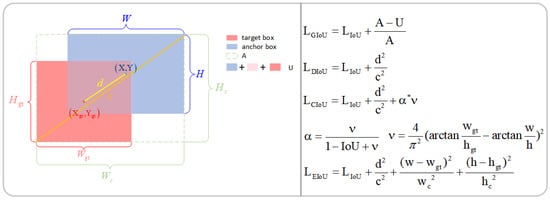
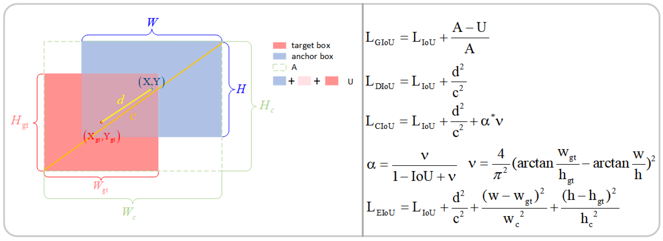
To overcome the inherent limitations of IoU in loss function design, numerous research efforts have been conducted to address its shortcomings, aiming to more effectively guide anchor boxes toward achieving accurate and efficient regression optimization. Figure 1 illustrates the structural designs of the GIoU, DIoU, CIoU, and EIoU loss functions. The Generalized Intersection over Union (GIoU) loss, denoted by $L_{\mathrm{GIoU}}$ [11], introduces a penalty term based on the area of the minimum enclosing rectangle to construct a penalty factor. Even when IoU equals 0, it can still provide an optimization direction through the area difference of the enclosing rectangle, but its ability to localize anchor boxes is insufficient. The Distance-IoU (DIoU) loss, denoted by $L_{\mathrm{DIoU}}$ [12], incorporates a penalty term for the distance between center points, with its core focusing on aligning the center points while neglecting the optimization of shape differences. The Complete IoU (CIoU) loss, denoted by $L_{\mathrm{CIoU}}$ [12], is built upon $L_{\mathrm{DIoU}}$ and adds an aspect-ratio penalty to account for shape differences, yet it fails to reflect the specific magnitude of such differences. The Efficient Intersection over Union (EIoU) loss, denoted by $L_{\mathrm{EIoU}}$ [13], uses center distance and width-height discrepancies as penalties to measure the differences between bounding boxes in a more refined manner. However, improper weighting leads to imbalanced optimization performance. The SCYLLA-IoU (SIoU) loss, denoted by $L_{\mathrm{SIoU}}$ [14], introduces an angle loss and uses angular constraints to guide the direction of bounding box regression. Nevertheless, when the size of the anchor box is larger than that of the target box, the shape loss cannot effectively characterize the differences. $L_{\mathrm{ShapeIoU}}$ [15] designs a size factor to enhance adaptability to target scales and achieve more refined shape matching, but it requires parameter tuning of the size factor according to different datasets, resulting in weak generalization.

Figure 1. Illustrations of the Generalized Intersection over Union (GIoU), Distance-IoU (DIoU), Complete IoU (CIoU), and Efficient Intersection over Union (EIoU) loss functions. The asterisk in the CIoU formula denotes multiplication.

Although related works have enhanced the representational capability of IoU, the inherent flaws of IoU itself remain unresolved, and issues also exist in the design of some penalty factors. To address this problem, this study proposes a diagonal-based loss function designed around bounding boxes. The contributions of this paper are as follows:

First, the research analyzes the design principles and structural characteristics of existing bounding box loss functions that employ IoU as the core component. It further investigates how the designs of IoU and penalty factors affect the convergence of anchor boxes, and proposes a novel approach that reconstructs the loss function using diagonals as an equivalent representation of anchor boxes. By transforming the traditional anchor box regression problem into a diagonal regression problem, this method provides a new modeling perspective and optimization pathway for anchor box regression tasks.

Second, a composite metric termed “$L_1+L_2$” is developed, integrating both difference measurement and optimization principles. Based on this metric, a diagonal-based loss function named Two-Point Loss (TPL) is formulated. The proposed TPL not only captures the discrepancies between anchor boxes with higher precision but also mitigates undesired variations during regression, thus enabling the diagonals to converge more accurately and efficiently.

Finally, an attention factor, denoted by $\beta$, is incorporated to construct TPLv2. This adaptive factor suppresses the excessive influence of low-quality anchor boxes during optimization, attenuates their gradient impact in backpropagation, and balances the contributions of high- and low-quality samples. As a result, the enhanced loss formulation significantly improves detection performance, particularly in small-object datasets.

2. Analysis of Bounding Box Regression Loss Functions

2.1. Penalty Factor Analysis

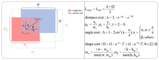
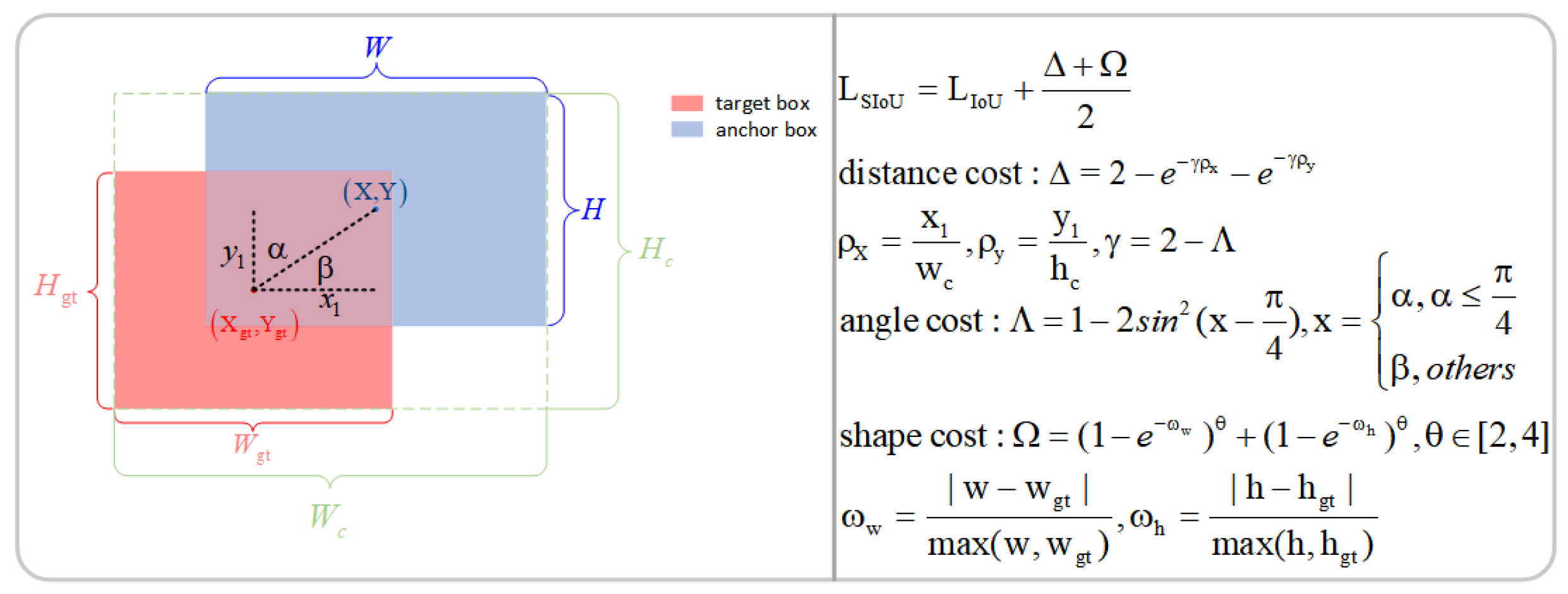
Current mainstream bounding box loss functions are constructed based on IoU. They have achieved certain results in improving the localization accuracy of object detection models, accelerating convergence, and enhancing adaptability to different object scales. However, some existing penalty factors still have deficiencies in their design, and these deficiencies provide important theoretical basis and practical experience for the optimization and improvement of subsequent loss functions. Figure 2 and Figure 3 illustrate the structures of the SIoU and ShapeIoU loss functions, respectively.

Figure 2. Illustration of the SIoU Loss Structure.

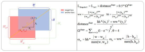
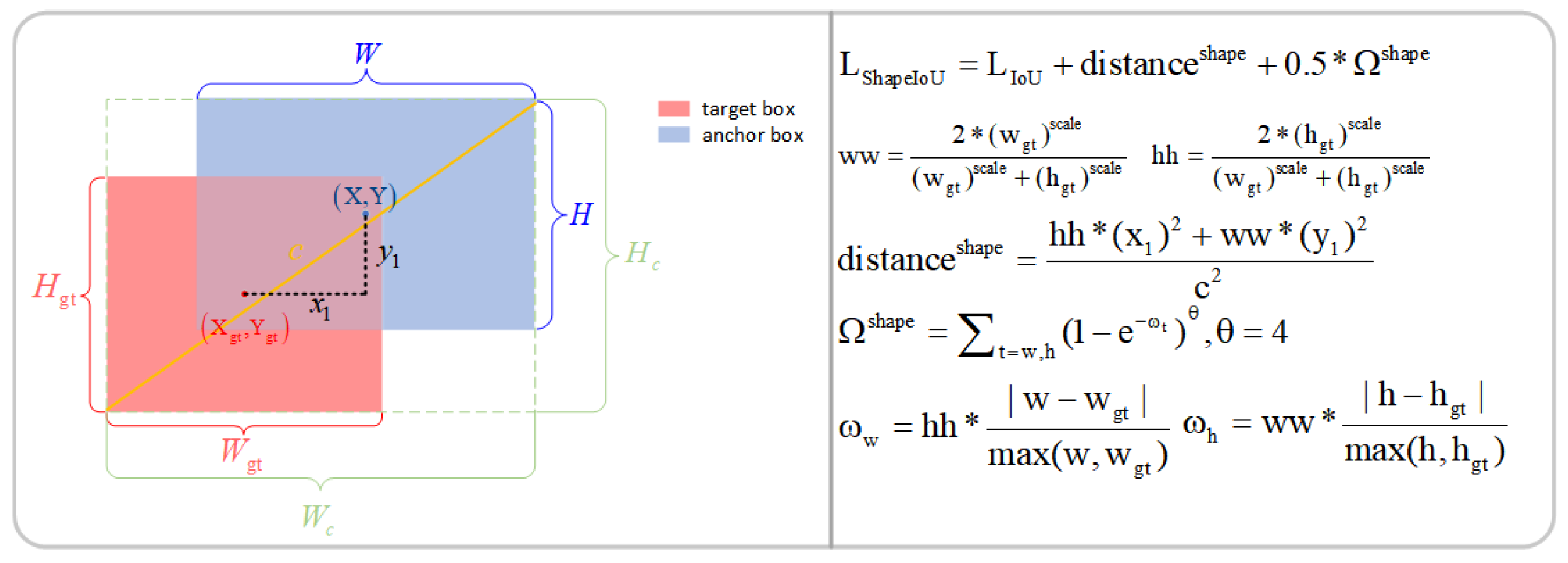
Figure 3. Illustration of the ShapeIoU Loss Structure. Asterisks in the displayed equations denote multiplication.

$L_{\mathrm{GIoU}}$: To address the gradient vanishing issue of IoU when there is no overlap between bounding boxes, $L_{\mathrm{GIoU}}$ proposes a penalty term ${\displaystyle \frac{A-U}{A}}$ [11]. However, when the predicted box is located inside the target box, $L_{\mathrm{GIoU}}$ degrades to $L_{\mathrm{IoU}}$ [12]. During the optimization process of the predicted box, expanding the predicted box will reduce the penalty term ${\displaystyle \frac{A-U}{A}}$, which significantly slows down the convergence speed. Therefore, the design of ${\displaystyle \frac{A-U}{A}}$ is unreasonable; the dynamic numerator and denominator lead to irrational gradients, causing the shape to be optimized in the opposite direction.

$L_{\mathrm{DIoU}}$:$L_{\mathrm{DIoU}}$ constructs a loss function around the center point distance and aspect ratio, and designs a penalty term ${\displaystyle \frac{d^2}{c^2}}$. The specific formula is ${\displaystyle \frac{{(X-X_{\mathrm{gt}})}^2+{(Y-Y_{\mathrm{gt}})}^2}{W_c^2+H_c^2}}$, and its gradients are shown in Equations (1) and (2). A negative gradient indicates that during the anchor box optimization process, the decrease in the values of $W_c$ and $H_c$ will cause $L_{\mathrm{DIoU}}$ to tend to increase. However, $W_c$ and $H_c$ should decrease along with $L_{\mathrm{DIoU}}$, which results in unexpected anchor box changes and hinders anchor box regression.

$${\displaystyle \frac{\partial L_{\mathrm{DIoU}}}{\partial W_c}}=-2W_c{\displaystyle \frac{{(w-w_{\mathrm{gt}})}^2+{(h-h_{\mathrm{gt}})}^2}{{(W_c^2+H_c^2)}^2}}<0$$

(1)

$${\displaystyle \frac{\partial L_{\mathrm{DIoU}}}{\partial H_c}}=-2H_c{\displaystyle \frac{{(w-w_{\mathrm{gt}})}^2+{(h-h_{\mathrm{gt}})}^2}{{(W_c^2+H_c^2)}^2}}<0$$

(2)

$L_{\mathrm{CIoU}}$: On the basis of $L_{\mathrm{DIoU}}$, $L_{\mathrm{CIoU}}$ adds a penalty term $\alpha v$, which incorporates the aspect ratio. The purpose is to guide the anchor box regression process to focus on the shape difference. However, for the penalty term v, ${\displaystyle \frac{\partial v}{\partial w}}$ and ${\displaystyle \frac{\partial v}{\partial h}}$ are positive and negative respectively [13], as shown in Equations (3) and (4). When w needs to increase or h needs to decrease, incorrect gradients are provided to v to promote its increase; The v is constructed based on the difference in aspect ratio, but it cannot truly reflect the length and width gap between the predicted box and the ground-truth box, and its effect on reducing the length and width difference is relatively limited.

$${\displaystyle \frac{\partial v}{\partial w}}={\displaystyle \frac{8}{{\pi }^2}}{\left({tan}^{-1}{\displaystyle \frac{w_{\mathrm{gt}}}{h_{\mathrm{gt}}}}-{tan}^{-1}{\displaystyle \frac{w}{h}}\right)}^2{\displaystyle \frac{h}{w^2+h^2}}$$

(3)

$${\displaystyle \frac{\partial v}{\partial h}}=-{\displaystyle \frac{8}{{\pi }^2}}{\left({tan}^{-1}{\displaystyle \frac{w_{\mathrm{gt}}}{h_{\mathrm{gt}}}}-{tan}^{-1}{\displaystyle \frac{w}{h}}\right)}^2{\displaystyle \frac{w}{w^2+h^2}}$$

(4)

$L_{\mathrm{EIoU}}$:$L_{\mathrm{EIoU}}$ abandons the aspect ratio and directly uses the length and width differences as penalties. However, during the regression process, the differences between the widths and heights of the two anchor boxes are much smaller than the length and width of the minimum enclosing box. Therefore, the values of ${(w-w_{\mathrm{gt}})}^2$ and ${(h-h_{\mathrm{gt}})}^2$ are far smaller than those of $w_c^2$ and $h_c^2$, resulting in excessively small values and gradients of the penalty term, which makes it unable to help adjust the shape of the predicted box [13]. Focal -EIoU designs a hyperparameter ${\mathrm{IoU}}^{\gamma }$. The loss values and gradients of low -quality samples will be significantly reduced due to the low IoU value. However, for anchor boxes with very poor quality (i.e., IoU = 0 or close to 0), the value of ${\mathrm{IoU}}^{\gamma }$ is also close to 0. At this time, anchor boxes with extremely poor quality are equivalent to those with extremely good quality, which will have a negative impact on model localization and anchor box optimization.

$L_{\mathrm{SIoU}}$:$L_{\mathrm{SIoU}}$ is constructed around the center point angle cost, distance cost, and shape cost. It guides the anchor box to regress at a specific angle, which greatly reduces the dispersion degree of anchor box regression and thus accelerates the convergence speed. Although it restricts the regression angle of the anchor box, the use of $w_c$ and $h_c$ as denominators in the distance loss leads to excessively small values, which cannot provide sufficient gradients for the regression of the center point distance. At the same time, for the shape loss, when w and h are larger than $w_{\mathrm{gt}}$ and $h_{\mathrm{gt}}$, the denominator lacks the information of the target box, making it insufficiently sensitive to the length and width of the target box and affecting the anchor box regression.

$L_{\mathrm{ShapeIoU}}$:$L_{\mathrm{ShapeIoU}}$ holds that the change in the short side of the anchor box has a greater impact on IoU than that of the long side, and the IoU value during the regression of small -scale bounding boxes is more significantly affected by the shape of the anchor box [15]. Therefore, this loss function adds a scale factor, but this scale factor needs to be adjusted according to different datasets to achieve the best effect, resulting in poor generalization. At the same time, in the design of ${\omega }_w$ and ${\omega }_h$, when w and h are larger than $w_{\mathrm{gt}}$ and $h_{\mathrm{gt}}$, the information of the target box is missing. In addition, in the distance loss, c is used as a denominator, which also leads to an excessively small gradient and affects the optimization effect.

2.2. Causes of Anchor Box Expansion

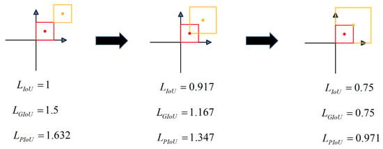
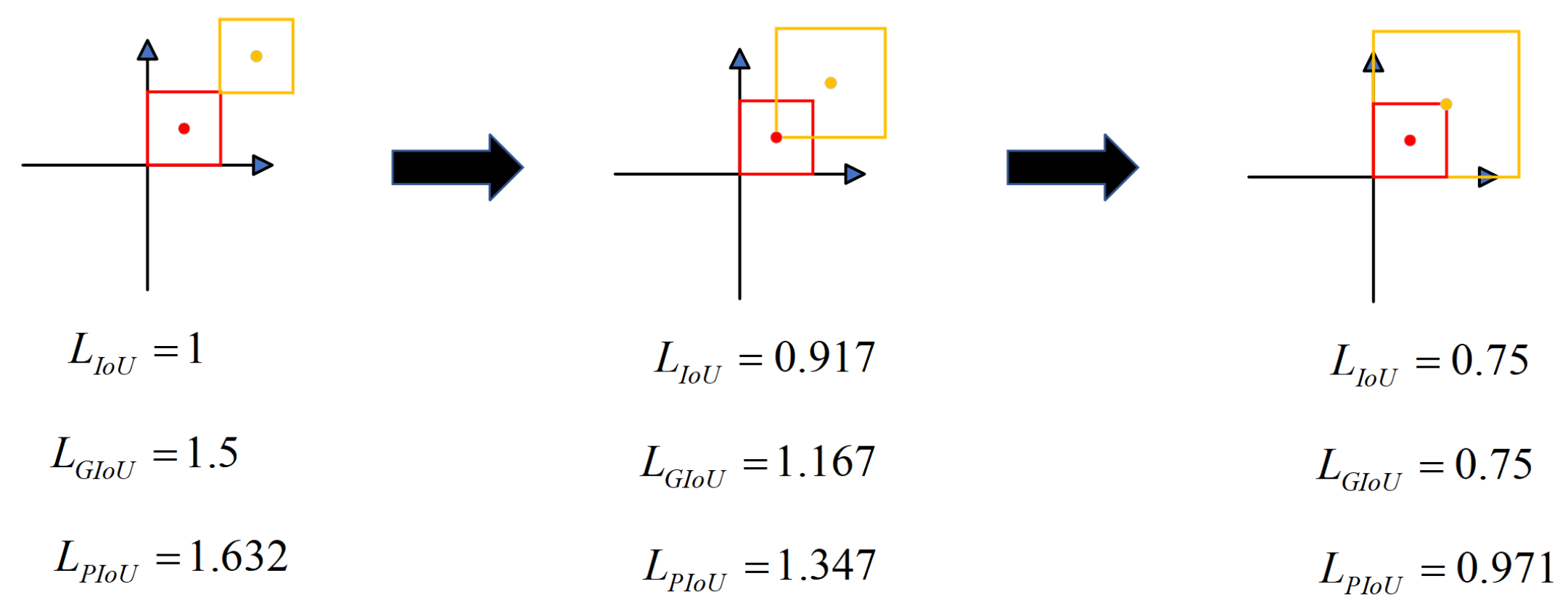
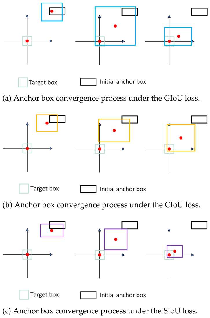
Under the influence of bounding box loss functions constructed based on IoU, anchor boxes often exhibit size expansion during the regression process. The fundamental reason lies in the fact that such loss functions are significantly less sensitive to shape information than to position information, and fail to provide reasonable gradient constraints for length and width. Consequently, when unintended changes occur in the shape of the bounding box, even if such changes only reduce the loss value without actually improving the matching quality, the optimization process may misjudge this as a correct direction, thereby leading to unintended expansion of the anchor box size. A simple example is used in Figure 4 to illustrate this phenomenon.

Figure 4. Variation of the loss value during the anchor box expansion process. The red box denotes the target box, and the yellow box denotes the evolving anchor box. The large right-pointing arrows show successive stages of expansion, while the black arrows indicate the coordinate axes.

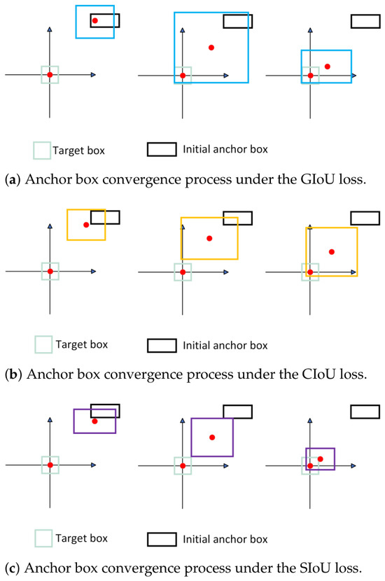
As shown in Figure 4, initially, the two anchor boxes only differ in position. As the anchor boxes expand, the distance between their center points gradually decreases; this change is in line with expectations. However, the shape change is irrational: the differences in their length and width gradually increase, while the corresponding loss value decreases. This result indicates that the change in shape information at this point provides incorrect gradients, allowing the irrational expansion of anchor boxes to still achieve optimization effects. Nevertheless, such changes will create obstacles for subsequent optimization and increase the time required for anchor box convergence. Although some loss functions developed after IoU have introduced penalty factors to attempt to modify such gradients, IoU itself inherently has this flaw and this is the reason why anchor boxes tend to undergo irrational changes. Figure 5 illustrates the convergence processes of GIoU, CIoU, and SIoU, respectively.

Figure 5. Anchor box regression pathways under different loss functions. The pale-green box denotes the target box, and the black box denotes the initial anchor box. The blue, yellow, and purple boxes show the evolving anchor boxes under GIoU, CIoU, and SIoU, respectively. Red dots mark box centers.

3. Construction of the Bounding Box Loss Function

3.1. Design of the Penalty Factor

The introduction of the penalty factor aims to more accurately measure the difference between the predicted bounding box and the ground-truth bounding box, while further refining the optimization direction of the anchor box. When designing the penalty factor, the following principles can be followed to ensure its effectiveness and robustness:

First, when constructing a penalty factor for a specific optimization objective, it is necessary to ensure that the partial derivative of the loss function with respect to this factor is consistent with the expected optimization direction. For example, if the penalty factor is constructed using the difference in width and height between two anchor boxes, considering that a reduction in the width-height difference helps improve the anchor box regression accuracy, the partial derivative of the loss function with respect to this difference should be positive. This ensures that their variation trends remain consistent, guarantees the effectiveness of gradient updates, and prevents the optimization effect from being diluted.

Second, the numerical difference of anchor boxes for large objects is significantly larger than that for small objects. To adapt to anchor boxes of different sizes, the penalty factor can be constructed in the form of a numerator and a denominator: the difference is used as the numerator, and scale-related information of the target box is selected for the denominator. This approach enhances adaptability to anchor boxes of different scales, helps suppress abnormal fluctuations in gradients, and makes the optimization process more stable.

Finally, for the penalty factor, reasonable weight design is crucial, as it directly affects the relative contribution of each gradient term in the loss function. If the weight is too large, it may suppress the optimization effect of other loss terms; conversely, if the weight is too small, it will be difficult to achieve an effective optimization effect.

3.2. Design of the Attention Factor

In actual training processes, small objects typically yield low detection accuracy due to complex backgrounds and limited available information. Consequently, small-object datasets generate a large number of low-quality anchor boxes during training. These low-quality anchor boxes are prone to being incorrectly assigned as positive samples, which contaminates the positive sample set, misleads the model into learning invalid features, and ultimately degrades the model’s detection accuracy. Furthermore, these low-quality anchor boxes often make the dominant contribution to optimization. Relevant studies [11] have shown that low-quality anchor boxes account for an excessively large proportion of gradients, thereby interfering with the optimization process of normal anchor boxes. To address this issue, a specific attention factor needs to be designed: on the one hand, it suppresses the harmful gradients generated by low-quality anchor boxes; on the other hand, it enhances the contribution of high-quality anchor boxes to the overall loss, improving optimization efficiency and accuracy.

The design of the attention factor is associated with the quality of anchor boxes. Low-quality anchor boxes correspond to attention factors with smaller values, which reduces the proportion of their loss values and weakens the impact of their gradients during backpropagation. In contrast, high-quality anchor boxes correspond to attention factors with larger values, which increases the proportion of their loss values and strengthens the contribution of their gradients to model updates, effectively guiding model convergence. Additionally, the attention factor is more suitable for scenarios with imbalanced anchor box quality. It is particularly necessary for training lightweight models with weak detection capabilities or small-object datasets with higher detection difficulty.

3.3. Morphological Transformation of the Loss Function

The bounding box loss function is constructed based on anchor box information and acts on anchor boxes. It must not only effectively reflect the degree of information difference between anchor boxes but also guide the reasonable optimization of anchor boxes. For an anchor box, its information composition consists of two parts: first, shape information, which is reflected in the width and height of the anchor box; second, position information, which is reflected in the position coordinates of the anchor box. Shape and position information jointly determine the complete representation of an anchor box and form the basis for the design and optimization of the bounding box loss function.

The diagonal of an anchor box contains both its shape information and position information, and thus can serve as an effective representation of the anchor box’s overall features. The information gap between diagonals can be converted into the information gap between anchor boxes. Therefore, a diagonal loss function can be constructed based on the difference between diagonals, providing a new possibility for the design of the bounding box loss function.

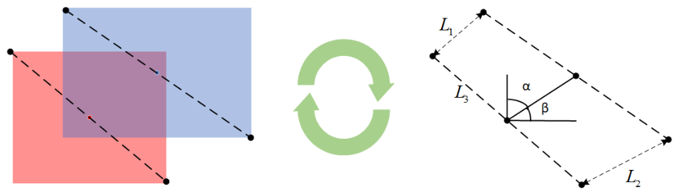
As an equivalent representation form of anchor boxes, diagonals can not only be the object of loss function optimization but also participate in the regression process as an optimization target. It should be noted that whether a diagonal loss function or a bounding box loss function is adopted, their essence lies in guiding the model to optimize the information of anchor boxes. The two are mutually convertible in terms of information representation; their difference lies in the change of optimization perspective: in the diagonal scheme, the optimization process no longer centers on anchor box parameters, but focuses on the difference between anchor box diagonals, breaking free from the limitation of using IoU as the measurement basis. At the level of optimization results, the target shifts from the traditional “anchor box overlap” to “diagonal overlap”. The two are theoretically equivalent but differ significantly in their construction methods, thereby providing a new optimization path for the model. The mutual conversion process between diagonals and anchor boxes is shown in Figure 6.

Figure 6. Mutual conversion between the anchor box and its diagonal representation. The red and blue boxes denote the target and anchor boxes, respectively. Dashed lines indicate their diagonals, and the green arrows indicate conversion between the box and diagonal representations.

4. Diagonal Loss Function TPL

4.1. Core of Construction

As a core component of the anchor box loss function, IoU is used to measure the overlap degree between the predicted box and the ground-truth box, and guides the position adjustment of anchor boxes. In the construction of the diagonal loss function, a core measurement element is also required, one that can not only effectively characterize the geometric difference between diagonals but also reasonably guide the optimization direction of anchor boxes.

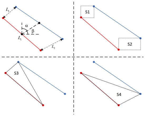
For a diagonal, the information that can represent its own attributes includes slope, length, center point coordinates, and so on. Among these, the position information of the two endpoints of a diagonal determines all its geometric attributes. Therefore, the difference in position information between the two endpoints is taken as the measurement index for evaluating the difference between two diagonals and as the object of optimization. As shown in Figure 6, L1 and L2 represent the distances between the top-left endpoints and the bottom-right endpoints (of the two diagonals), respectively. The larger the values of L1 and L2, the greater the difference between the two diagonals becomes, as can be approximately verified; when the values of L1 and L2 approach zero, the two diagonals tend to coincide.

4.2. Proposal of TPL

TPL is a diagonal loss function that drives diagonal regression. Its design concept is to drive the coincidence of the two endpoints of the diagonal, i.e., the sum of L1 and L2 equals zero. The specific formulas are shown in Equations (5)–(10):

$$L_{TPL}=1-e^{-\gamma d}+1-e^{-S}$$

(5)

$$d={\displaystyle \frac{L_1/L_3+L_2/L_3}{2}}$$

(6)

$$L_1=\sqrt{{(X_1-X_{\mathrm{gt}1})}^2+{(Y_1-Y_{\mathrm{gt}1})}^2}$$

(7)

$$L_2=\sqrt{{(X_2-X_{\mathrm{gt}2})}^2+{(Y_2-Y_{\mathrm{gt}2})}^2}$$

(8)

$$\gamma ={cos}^2\left({\displaystyle \frac{4\theta }{\pi }}\right)+1,\theta =\left\{\begin{array}{cc}\alpha ,\hfill & \alpha \le {\displaystyle \frac{\pi }{4}}\hfill \\ \beta ,\hfill & \mathrm{others}\hfill \end{array}\right.$$

(9)

$$S={\displaystyle \frac{2(S_1+S_2+S_3+S_4)}{S_{gt}}}$$

(10)

As illustrated in Figure 7, TPL consists of a distance loss and an area loss. Specifically, $1-e^{-\gamma d}$ represents the distance loss, while $1-e^{-S}$ represents the area loss. The distance term d is constructed from $L_1$, $L_2$, and $L_3$. Here, $L_1$ denotes the Euclidean distance between the top-left vertices of the two bounding boxes, $L_2$ denotes the Euclidean distance between their bottom-right vertices, and $L_3$ denotes the diagonal length of the ground-truth box. The area term S consists of $S_1$, $S_2$, $S_3$, and $S_4$. Specifically, $S_1$ and $S_2$ represent the areas of the squares constructed from the top-left vertices and bottom-right vertices of the two bounding boxes, respectively. Moreover, $S_3$ and $S_4$ represent the areas of the triangles formed by the top-left and bottom-right vertices of the predicted box, respectively, together with the diagonal of the ground-truth box. The factor $\gamma$ represents the angular loss, and $\theta$ takes the smaller value of $\alpha$ and $\beta$. Here, $\alpha$ and $\beta$ denote the angles between the line connecting the center points of the predicted and ground-truth boxes and the horizontal and vertical axes, respectively.

Figure 7. Composition of the TPL loss function. The red and blue line segments denote the target-box and anchor-box diagonals. Black dashed lines show auxiliary geometric constructions. S1 and S2 represent the areas of the squares constructed from the top-left vertices and bottom-right vertices of the two bounding boxes, respectively. Moreover, S3 and S4 represent the areas of the triangles formed by the top-left and bottom-right vertices of the predicted box, respectively, together with the diagonal of the ground-truth box.

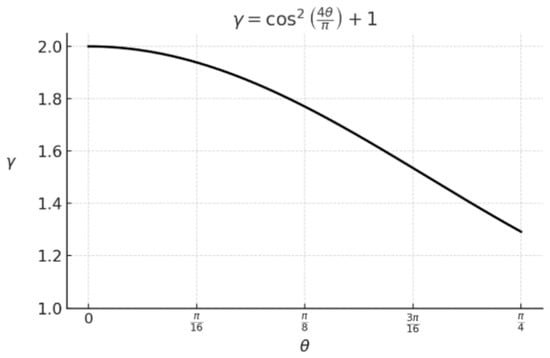
In the penalty term $1-e^{-\gamma d}$, d is the core quantity to be optimized. The denominator $L_3$ enables the loss to better adapt to targets of different sizes. By constraining the regression of the center point to an approximately consistent direction, $\gamma$ guides $L_1$ and $L_2$ to decrease rapidly, thereby reducing unnecessary dispersion. For $\gamma$, when $\theta$ approaches 0, $\gamma$ approaches its maximum value of 2, while the magnitude of its gradient approaches 0. When $\theta$ approaches ${\displaystyle \frac{\pi }{4}}$, $\gamma$ approaches its minimum value, and the magnitude of its gradient also gradually decreases. Within the intermediate range, the gradient magnitude first increases gradually, reaches its maximum value, and then decreases. The variation curve of $\gamma$ is shown in Figure 8.

Figure 8. Amplitude curve of $\gamma$ with respect to $\theta$.

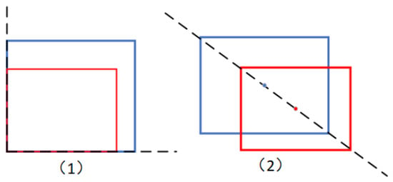
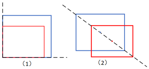
Since the distance loss can only reflect the endpoint distance and lacks detailed positional information, the area loss $1-e^{-\varsigma S}$ is designed to complement this deficiency by incorporating spatial cues. In this formulation, $S_{gt}$ denotes the area of the ground-truth bounding box, while $S_1$, $S_2$, $S_3$, and $S_4$ represent the corresponding subregions as illustrated in Figure 7. Specifically, $S_1$ and $S_2$ are designed to compensate for the missing positional information in $L_1$ and $L_2$, whereas $S_3$ and $S_4$ further refine this spatial compensation, effectively avoiding potential issues arising from missing information in special cases. Figure 9 illustrates two representative cases: in case (1), $S_1$ and $S_2$ vanish, and $S_3$ and $S_4$ become dominant; conversely, in case (2), $S_1$ and $S_2$ play the primary roles. This mutual compensation mechanism ensures the robustness of the loss function under various degenerate conditions and enhances its adaptability across different scenarios.

Figure 9. Two special cases: (1) two edges of the bounding boxes are aligned on the same straight line; (2) the diagonal lines of the bounding boxes lie on the same straight line. The red outline denotes the target box, and the blue outline denotes the regressed anchor box. Dashed lines highlight their special positional relationship.

From the perspective of gradient behavior, TPL maintains positive derivatives with respect to both the distance loss and the area loss. This ensures the consistency and stability of the optimization process, as shown in Equations (11) and (12):

$${\displaystyle \frac{\partial \mathrm{TPL}}{\partial d}}=\gamma e^{-\gamma d}>0$$

(11)

$${\displaystyle \frac{\partial \mathrm{TPL}}{\partial S}}=e^{-S}>0$$

(12)

It is worth noting that $L_1+L_2$ constitutes the optimization core of TPL. The distance loss d is derived based on the structure of $L_1+L_2$, whereas the area loss S does not directly depend on their values. Nevertheless, its formulation compensates for the missing positional information of $L_1$ and $L_2$, thereby enhancing the model’s ability to capture angular deviations under various conditions. This design facilitates faster and more accurate convergence in bounding box angle regression.

4.3. TPLv2

TPL effectively balances the discrepancies among bounding boxes of varying quality. However, it is still challenging to mitigate the negative impact introduced by poor-quality bounding boxes with large localization deviations, especially in complex small-object detection tasks. These low-quality samples often contribute harmful gradients during optimization, leading the model to learn ineffective or misleading features. To address this issue, all bounding boxes, regardless of their quality, should receive appropriate attention during optimization. This allows the loss function to focus more effectively on the optimization of $L_1+L_2$. On this basis, an improved version, denoted as TPLv2, is proposed in this study, which introduces an additional attention factor $\beta$ to refine the weighting of bounding box contributions, as defined in Equations (13)–(15):

$$L_{TPLv2}=\beta ·L_{TPL}$$

(13)

$$\beta =2e^{-d},$$

(14)

$$d={\displaystyle \frac{L1/L3+L2/L3}{2}}.$$

(15)

In $L_{TPLv2}$, $\beta$ is constructed based on $L1+L2$. For high-quality anchor boxes, d has a smaller value, resulting in a larger $\beta$ that enhances their optimization contribution. Conversely, for low-quality anchor boxes, d becomes larger and $\beta$ decreases, suppressing their optimization contribution. When $\beta$ acts adaptively, the gradient disparity between high- and low-quality anchor boxes is effectively balanced, reducing the adverse effects of poor-quality anchors and maintaining a stable and efficient optimization process.

5. Experiment

5.1. Design of Experiment

Dataset Selection: The VisDrone2019 dataset is a public dataset released by Tianjin University, consisting of images captured by unmanned aerial vehicles (UAVs) across different locations, altitudes, times, and weather conditions. Specifically, it includes 6471 images in the training set, 548 images in the validation set, and 1610 images in the test set. The detection targets cover a total of ten categories, such as pedestrians, bicycles, and cars, with the total number of objects exceeding 540,000. The DOTA dataset is a remote sensing image object detection dataset, which is widely used in tasks like remote sensing image analysis and target localization. It contains 11,268 high-resolution remote sensing images, with detection targets including 18 categories such as aircraft, vehicles, and ships. This dataset is characterized by dense target aggregation and large-scale variations.

Model Selection: YOLOv11, YOLOv12, and Real-Time Detection Transformer (RT-DETR) are currently advanced object detection models. Among them, YOLOv11 incorporates new components such as C3k2 blocks and C2PSA, which facilitate more effective feature extraction and processing. Centered on the attention mechanism, YOLOv12 establishes an efficient and straightforward YOLO framework, breaking the dominant position of CNNs in YOLO. RT-DETR, on the other hand, is an object detection algorithm based on the Transformer architecture. Despite its excellent detection accuracy, it exhibits relatively slow inference speed.

5.2. Experimental Environment and Metrics

The experiments were conducted on an Ubuntu 20.04 operating system. The environment configuration was as follows: Python version 3.8, CUDA version 11.8, and PyTorch version 2.0. The hardware setup included a 14-core Intel(R) Xeon(R) Platinum 8362 CPU @ 2.80 GHz and a single NVIDIA RTX 3090 GPU with 24 GB of memory. During training, the Adam optimizer was employed, with a learning rate $\left(lr\right)$ of 0.01 and a learning rate decay parameter $\left(lrf\right)$ set to 0.01. The batch size was set to 16, and the input image resolution was $640\times 640$. The total number of training epochs was set to 200.

For performance evaluation, the metrics mAP@0.5 and mAP@0.5:0.95 were adopted. Specifically, mAP@0.5 denotes the mean Average Precision (mAP) at an IoU threshold is 0.5. mAP@0.5:0.95 represents the mean value of Average Precision (AP) calculated at IoU thresholds ranging from 0.5 to 0.95 with a step size of 0.05. Here, AP refers to the average precision of each individual category. The formula for mAP is expressed as:

$$\mathrm{mAP}={\displaystyle \frac{{\sum }_{i=1}^{N}A{P}_i}{N}}.$$

(16)

5.3. Ablation Study

In TPL, each loss term contributes to bounding box regression. To directly evaluate the improvement in detection accuracy introduced by each loss term, an ablation study was conducted using YOLOv11s on the VisDrone2019 dataset. The experimental results are presented in Table 1.

Table 1. Ablation study of the loss terms in TPL.

Loss Term	mAP@0.5	mAP@0.5:0.95
d	0.320	0.178
$1-e^{-d}$	0.360	0.201
$1-e^{-\gamma d}$	0.368	0.212
$1-e^{-\gamma d}+1-e^{-S}$	0.372	0.214

5.4. Comparative Experiments

To validate the effectiveness of the proposed angular loss function, a series of comparative experiments were conducted between the proposed loss function and the mainstream loss functions based on the IoU metric. All other experimental settings were kept identical to ensure fairness. Table 2, Table 3 and Table 4 present the results on the VisDrone2019 dataset, where the models YOLOv11s, YOLOv12s, and RT-DETR were employed, respectively. Table 5 shows the results obtained by training YOLOv11s on the DOTA dataset. The experimental results are summarized as follows.

Table 2. The results of comparison experiments of YOLOv11s on the Visdrone2019 dataset.

Method	P	R	Map@0.5	Map@0.5:0.95
CIoU	0.494	0.362	0.369	0.212
DIoU	0.488	0.375	0.373	0.216
GIoU	0.496	0.365	0.370	0.213
SIoU	0.495	0.367	0.371	0.213
MPDIoU [16]	0.497	0.365	0.371	0.214
WIoU [17]	0.493	0.359	0.369	0.213
ShapeIoU	0.493	0.365	0.372	0.214
PIoU [18]	0.495	0.363	0.371	0.215
NWD Loss [19]	0.493	0.366	0.372	0.214
WIoU v3 [17]	0.495	0.363	0.371	0.214
TPL	0.494	0.364	0.372	0.214
TPLv2	0.498	0.362	0.375	0.217

Table 3. The results of comparison experiments of YOLOv12s on the Visdrone2019 dataset.

Method	P	R	Map@0.5	Map@0.5:0.95
CIoU	0.489	0.366	0.371	0.215
DIoU	0.484	0.366	0.373	0.216
GIoU	0.481	0.365	0.370	0.214
SIoU	0.494	0.365	0.371	0.215
MPDIoU	0.495	0.363	0.369	0.211
WIoU	0.492	0.363	0.370	0.215
ShapeIoU	0.479	0.367	0.370	0.214
PIoU	0.502	0.367	0.374	0.216
NWD Loss	0.496	0.365	0.373	0.216
WIoU v3	0.498	0.364	0.373	0.215
TPL	0.497	0.363	0.374	0.216
TPLv2	0.478	0.371	0.376	0.219

Table 4. The results of comparison experiments of RT-DETR on the VisDrone2019 dataset.

Method	P	R	Map@0.5	Map@0.5:0.95
CIoU	0.607	0.464	0.476	0.294
DIoU	0.602	0.465	0.473	0.293
GIoU	0.605	0.464	0.475	0.293
SIoU	0.612	0.464	0.476	0.296
MPDIoU	0.607	0.461	0.474	0.293
WIoU	0.607	0.463	0.476	0.294
ShapeIoU	0.601	0.459	0.471	0.290
PIoU	0.611	0.465	0.473	0.292
NWD Loss	0.610	0.466	0.476	0.294
WIoU v3	0.609	0.467	0.476	0.295
TPL	0.609	0.468	0.476	0.293
TPLv2	0.608	0.468	0.477	0.295

Table 5. The results of comparison experiments of YOLOv11s on the DOTA dataset.

Method	P	R	Map@0.5	Map@0.5:0.95
CIoU	0.777	0.663	0.707	0.478
DIoU	0.776	0.660	0.709	0.477
GIoU	0.795	0.646	0.707	0.478
SIoU	0.794	0.651	0.711	0.478
MPDIoU	0.771	0.668	0.711	0.479
WIoU	0.777	0.660	0.710	0.478
ShapeIoU	0.801	0.653	0.711	0.479
PIoU	0.786	0.668	0.712	0.481
NWD Loss	0.784	0.668	0.712	0.480
WIoU v3	0.782	0.670	0.711	0.480
TPL	0.783	0.669	0.712	0.480
TPLv2	0.762	0.647	0.701	0.471

As shown in the tables, experiments conducted on the VisDrone2019 dataset demonstrate that, regardless of the model used—YOLOv11s, YOLOv12s, or RT-DETR—the proposed TPL consistently outperforms the baselines in both mAP@0.5 and mAP@0.5:0.95 metrics. Moreover, TPLv2 achieves further improvements over TPL on these indicators, yielding superior detection results. However, when tested on the high-precision DOTA dataset, the accuracy of TPLv2 declines noticeably, whereas TPL maintains stable performance. This indicates that the introduction of the attention factor $\beta$ is not universally applicable to all datasets, and it performs better on datasets with lower detection accuracy, where it enhances the optimization contribution of lower-quality bounding boxes.

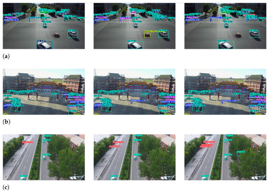
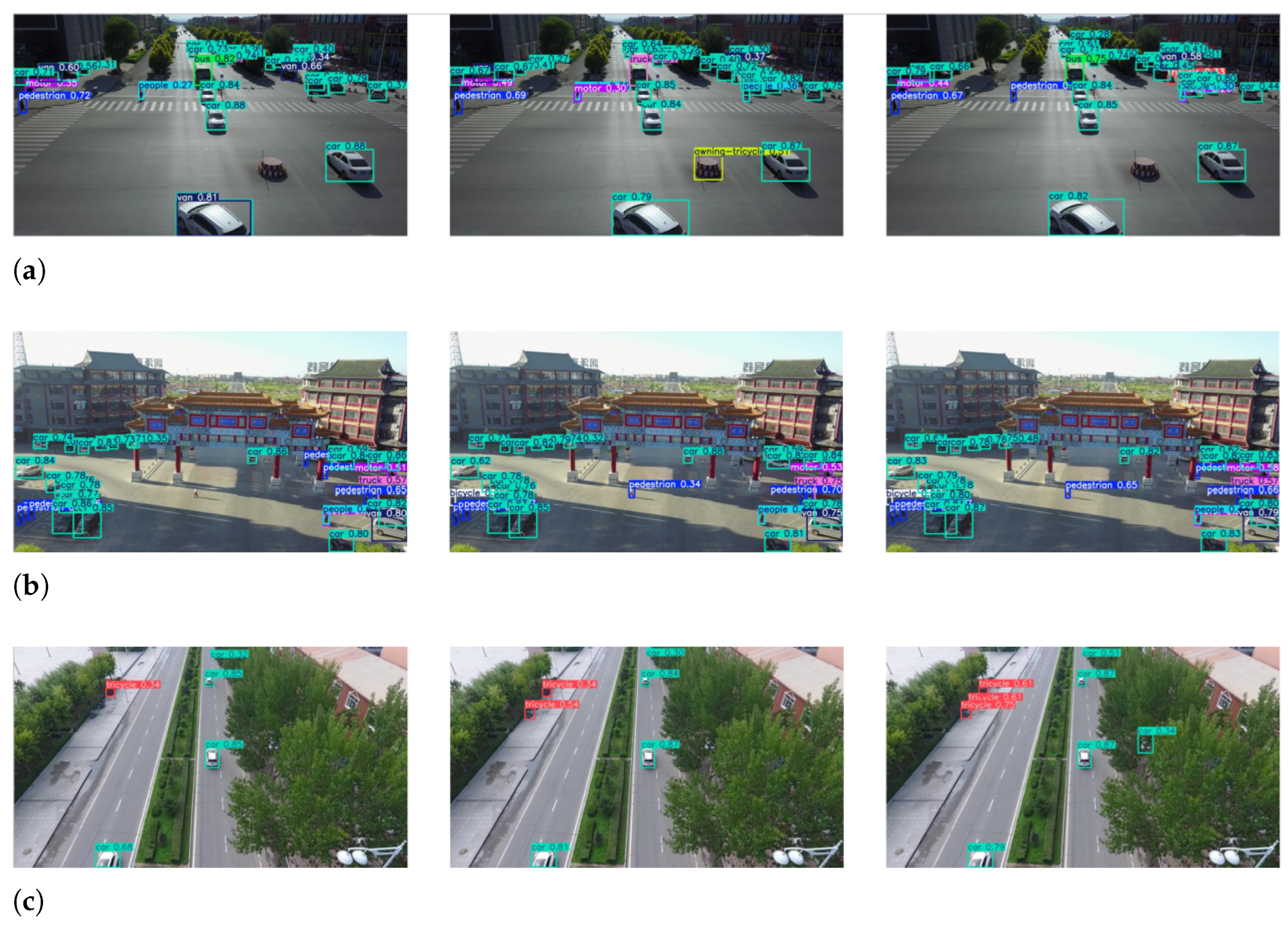
To further visualize the improvement in detection performance, additional experiments were conducted under strictly consistent settings, using YOLOv11s trained on the VisDrone2019 dataset while only modifying the underlying loss functions. Specifically, PIoU and ShapeIoU were selected as comparison methods, and the corresponding detection results are illustrated in Figure 10.

Figure 10. The detection results of YOLOv11s on the VisDrone2019 dataset are presented from top to bottom as follows: PIoU, ShapeIoU, and TPLv2.

As shown in Figure 10, in Group a: the car at the bottom of the left image is misdetected as a pickup truck, the traffic platform in the middle image is misdetected as a sunshade tricycle, while all targets in the right image are correctly detected. In Group b: the pedestrian on the central road in the first image and the pedestrian next to the 4th pillar (counting from left to right) in the second image are missed, whereas all targets in the third image are detected. In Group c: the electric tricycle at the top-left corner and the car on the right side of the road (obscured by trees) are missed in the first and second images, but successfully detected in the third image. It can be concluded that the diagonal loss function proposed in this paper can effectively reduce the phenomena of missing detection and misdetection in small object detection tasks, thereby improving the detection accuracy of the model.

5.5. Experimental Analysis

From the experimental results, it can be observed that the performance of different loss functions varies significantly across different model architectures and datasets. TPL demonstrates relatively superior performance in comparison with current mainstream loss functions, exhibiting good generalization ability. In contrast, TPLv2, which incorporates an attention factor, shows stronger adaptability and robustness when dealing with datasets with low detection accuracy, indicating its potential advantages in such scenarios.

In practical applications, suppose that in the TPL loss function, the weighting factor of $(S_1+S_2)$ is denoted as ${\lambda }_1$, and that of $(S_3+S_4)$ is denoted as ${\lambda }_2$. Changes in the values of ${\lambda }_1$ and ${\lambda }_2$ have a significant impact on the experimental results. To analyze this effect, ablation experiments were conducted using YOLOv11s on the VisDrone2019 dataset, and the results are presented in Table 6.

Table 6. Ablation experiments of ${\lambda }_1$ and ${\lambda }_2$.

${\mathit{\lambda }}_1$	${\mathit{\lambda }}_2$	${\mathbf{mAP}}_{0.5}$	${\mathbf{mAP}}_{0.5:0.95}$
2.0	2.0	0.372	0.214
2.0	1.1	0.374	0.216
2.1	1.1	0.374	0.215
2.1	1.2	0.372	0.215
2.0	1.3	0.367	0.211

6. Conclusions

Bounding box loss functions constructed based on IoU tend to cause anchor box expansion. Meanwhile, the design of some penalty factors may also lead to incorrect anchor box regression. To further improve the accuracy of anchor box regression guided by bounding box loss functions, this paper first discusses the design flaws of certain penalty factors, analyzes the causes of anchor box expansion, and summarizes the design methods of penalty factors. These efforts provide insights for subsequent loss function design and can effectively reduce unintended changes in anchor boxes.

Second, this paper proposes a design method that replaces anchor boxes with diagonals, converting the traditional bounding box regression problem into a diagonal regression problem. By substituting the bounding box loss function with a diagonal loss function, a new solution for loss function design is provided. Based on this transformation idea, the diagonal loss function TPL is proposed. This function takes the difference in position information between two endpoints as the core to construct the loss and further builds penalty factors using these two endpoints, enabling efficient anchor box regression.

Finally, an attention factor is added to TPLv2 to address the imbalance in optimization contributions among anchor boxes of varying quality, effectively alleviating the difficulty of small object detection. Through comparative experiments on state-of-the-art object detection models and across datasets with objects of different sizes, the proposed diagonal loss functions TPL and TPLv2 achieve promising accuracy. Additionally, they offer a new perspective for future loss function design: using diagonal loss functions instead of anchor box loss functions for anchor box optimization.

References

- He, K.; Zhang, X.; Ren, S.; Sun, J. Deep residual learning for image recognition. In Proceedings of the IEEE Conference on Computer Vision and Pattern Recognition, Las Vegas, NV, USA, 27–30 June 2016; pp. 770–778. [Google Scholar]
- Vaswani, A.; Shazeer, N.; Parmar, N.; Uszkoreit, J.; Jones, L.; Gomez, A.N.; Kaiser, L.; Polosukhin, I. Attention is all you need. In Proceedings of the Advances in Neural Information Processing Systems, Long Beach, CA, USA, 4–9 December 2017; Volume 30. [Google Scholar]
- Gu, A.; Dao, T. Mamba: Linear-time sequence modeling with selective state spaces. arXiv 2023, arXiv:2312.00752. [Google Scholar]
- Wang, J.; Bi, L.; Ma, X.; Sun, P. An efficient YOLOX-based method for photovoltaic cell defect detection. Instrumentation 2024, 11, 83–94. [Google Scholar] [CrossRef] [Scilit]
- Chu, H.; Wang, T.; Miao, Q.; Chen, Z.; Wang, R.; Li, W.; Huang, T. Ship detection based on improved SDD algorithm. Instrumentation 2024, 11, 35–43. [Google Scholar]
- Liu, Y.; Li, T.; Zhou, Z.; Ren, W.; Lin, W. Real-world nighttime image dehazing via Bayesian-based fractional-order variational model. IEEE Trans. Image Process. 2026, 35, 4673–4685. [Google Scholar] [CrossRef] [Scilit] [PubMed]
- Li, C.; Zhou, H.; Liu, Y.; Yang, C.; Xie, Y.; Li, Z.; Zhu, L. Detection-friendly dehazing: Object detection in real-world hazy scenes. IEEE Trans. Pattern Anal. Mach. Intell. 2023, 45, 8284–8295. [Google Scholar] [CrossRef] [Scilit] [PubMed]
- Girshick, R. Fast R-CNN. In Proceedings of the IEEE International Conference on Computer Vision, Santiago, Chile, 7–13 December 2015; pp. 1440–1448. [Google Scholar]
- Ren, S.; He, K.; Girshick, R.; Sun, J. Faster R-CNN: Towards real-time object detection with region proposal networks. In Proceedings of the Advances in Neural Information Processing Systems, Montreal, QC, Canada, 7–12 December 2015; Volume 28. [Google Scholar]
- Yu, J.; Jiang, Y.; Wang, Z.; Cao, Z.; Huang, T. UnitBox: An advanced object detection network. In Proceedings of the 24th ACM International Conference on Multimedia, Amsterdam, The Netherlands, 15–19 October 2016; pp. 516–520. [Google Scholar]
- Rezatofighi, H.; Tsoi, N.; Gwak, J.Y.; Sadeghian, A.; Reid, I.; Savarese, S. Generalized intersection over union: A metric and a loss for bounding box regression. In Proceedings of the IEEE/CVF Conference on Computer Vision and Pattern Recognition, Long Beach, CA, USA, 15–20 June 2019; pp. 658–666. [Google Scholar]
- Zheng, Z.; Wang, P.; Liu, W.; Li, J.; Ye, R.; Ren, D. Distance-IoU loss: Faster and better learning for bounding box regression. In Proceedings of the AAAI Conference on Artificial Intelligence, New York, NY, USA, 7–12 February 2020; Volume 34, pp. 12993–13000. [Google Scholar]
- Zhang, Y.F.; Ren, W.; Zhang, Z.; Jia, Z.; Wang, L.; Tan, T. Focal and efficient IoU loss for accurate bounding box regression. Neurocomputing 2022, 506, 146–157. [Google Scholar] [CrossRef] [Scilit]
- Gevorgyan, Z. SIoU loss: More powerful learning for bounding box regression. arXiv 2022, arXiv:2205.12740. [Google Scholar]
- Zhang, H.; Zhang, S. Shape-IoU: More accurate metric considering bounding box shape and scale. arXiv 2023, arXiv:2312.17663. [Google Scholar]
- Ma, S.; Xu, Y. MPDIoU: A loss for efficient and accurate bounding box regression. arXiv 2023, arXiv:2307.07662. [Google Scholar]
- Tong, Z.; Chen, Y.; Xu, Z.; Yu, R. Wise-IoU: Bounding box regression loss with dynamic focusing mechanism. arXiv 2023, arXiv:2301.10051. [Google Scholar]
- Liu, C.; Wang, K.; Li, Q.; Zhao, F.; Zhao, K.; Ma, H. Powerful-IoU: More straightforward and faster bounding box regression loss with a nonmonotonic focusing mechanism. Neural Netw. 2024, 170, 276–284. [Google Scholar] [CrossRef] [Scilit] [PubMed]
- Wang, J.; Yuan, Y.; Yu, G. Normalized Wasserstein distance for accurate bounding box regression. Pattern Recognit. 2023, 137, 109295. [Google Scholar]
Disclaimer/Publisher’s Note: The statements, opinions and data contained in all publications are solely those of the individual author(s) and contributor(s) and not of MDPI and/or the editor(s). MDPI and/or the editor(s) disclaim responsibility for any injury to people or property resulting from any ideas, methods, instructions or products referred to in the content. |
© 2026 by the authors. Licensee MDPI, Basel, Switzerland. This article is an open access article distributed under the terms and conditions of the Creative Commons Attribution (CC BY) license.