A Shadow Price-Guided Computational Framework for Congestion-Aware Transmission Expansion Planning

Abstract

Transmission expansion planning (TEP) for renewable-rich power systems requires a computational workflow that links investment decisions with chronological operations and nodal economic signals. This study presents a shadow price-guided framework integrating hourly DC optimal power flow, multi-hour candidate screening, mixed-integer TEP, SCUC–SCED evaluation, and leave-one-line-out line value evaluation. Renewable curtailment is represented explicitly at renewable generators and is separated from involuntary load shedding. The SP-WCI candidate score aggregates 24 hourly flow–price difference products using congestion surplus weights. On a 101-bus reduced system, the automatically selected eight-line plan lowers average LMP from 597.33 to 259.98 CNY/MWh (56.5%), load shedding from 21,159.0 to 0.0 MWh (100.0%), and unused renewable/hydro availability from 117,882.9 to 50,398.7 MWh (57.2%). Comparison with weighted overload and rule-based screening uses the same candidate budget, while the random benchmark is summarized over ten independent seeds. Sensitivity tests show how the fixed plan responds to alternative load-shedding penalties. The complete screening–optimization–verification chain is additionally executed natively on the full-order 796-bus system, confirming that the framework scales to full network data while delineating the limits of the reduced surrogate. The results are interpreted as evidence from a stressed representative day case rather than as a general estimate of commercial project returns.

1. Introduction

The rapid integration of wind, solar, and hydro generation has turned transmission expansion planning (TEP) into a tightly coupled planning and operation problem. In renewable-rich grids, a candidate corridor changes not only branch loading but also commitment decisions, dispatch feasibility, locational marginal prices (LMPs), load shedding, and renewable curtailment [1,2]. A useful planning tool must, therefore, exchange information across optimization layers and retain the economic meaning of network constraints instead of treating expansion as an isolated capacity addition task.

From a planning perspective, this coupling creates four sequential questions. The planner must first determine where reinforcement should be considered and then identify which subset of corridors should be built, verify whether the selected topology remains effective under commitment and dispatch constraints, and finally determine whether the contribution of each individual line is consistent with the system-level result. Treating these questions separately can introduce an information discontinuity: a corridor may be screened by loading, selected by an investment model, and evaluated by a market model that uses different assumptions. The present framework is designed to maintain a common network representation and a common set of economic signals across all four decisions.

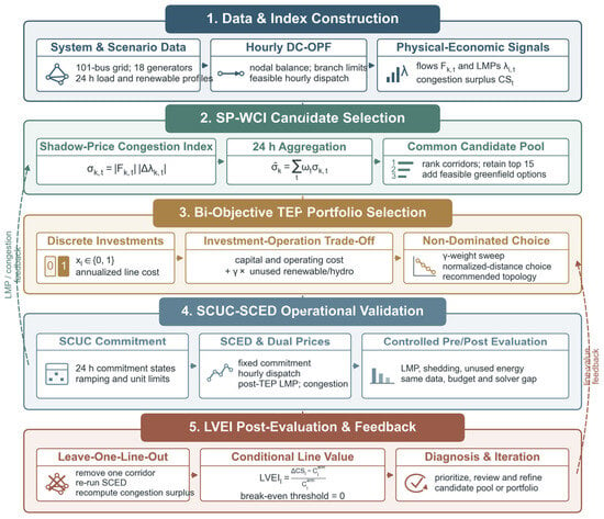
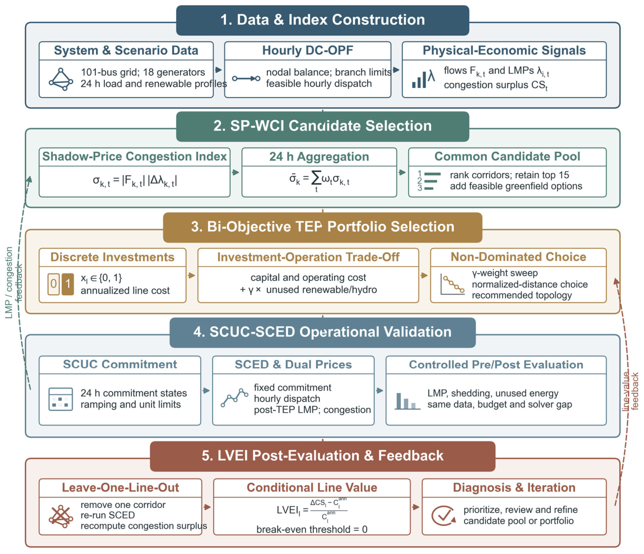
The framework proceeds through five stages: data and index construction, SP-WCI-based candidate line selection, bi-objective TEP, SCUC–SCED operational evaluation, and LVEI post-evaluation. A dual closed-loop feedback between LMP and congestion surplus links planning decisions back to candidate screening and forward to ex post line valuation.

The TEP literature spans deterministic DC formulations, stochastic and robust planning, and multi-stage co-planning models [3,4,5,6,7,8,9,10,11,12,13,14,15]. Multi-objective formulations expose risk, cost, and renewable integration trade-offs [13,16], while co-optimization and market coordination studies connect transmission decisions with generation and operational outcomes [17,18,19]. These advances motivate a workflow in which candidate generation, portfolio choice, and operational validation use consistent network and economic signals.

These three streams primarily improve the optimization model after a candidate set has already been supplied. Candidate generation itself receives less attention, even though it controls the search space of the subsequent MILP and can, therefore, predetermine which investment patterns are reachable. A small candidate set improves tractability but risks excluding high-value corridors, whereas an excessively broad set increases the binary search space and weakens interpretability. Candidate screening is consequently not a preliminary data-cleaning step; it is an integral part of the planning model and should be evaluated under the same operational conditions as the final expansion plan.

Market-based TEP provides an additional perspective because congestion is expressed through both physical loading and nodal price separation [12,20]. Thermal utilization alone indicates proximity to an engineering limit, but it does not measure the system cost of that limitation. Conversely, an LMP difference identifies economic separation but can be misleading on a lightly used corridor. A product of flow magnitude and absolute nodal price difference, therefore, offers a natural bridge between the engineering and market views of congestion. This observation motivates SP-WCI and distinguishes the proposed screening stage from approaches based solely on loading ratios or planner experience.

Despite these advances, candidate corridor construction is often external to the optimization, curtailment is sometimes inferred from generic feasibility slacks, and individual selected lines are rarely re-tested after portfolio optimization. These gaps can obscure whether a result comes from the candidate pool, the planning objective, or the operational redispatch. The present study addresses these issues through traceable multi-hour screening, explicit generator-level curtailment, and conditional leave-one-line-out diagnosis [21].

LMP is the dual variable of nodal active power balance and carries both marginal production cost and congestion information [20,22]. This interpretation underpins market-oriented expansion planning [23]. Multiplying the absolute endpoint LMP difference by absolute line flow gives an economically weighted congestion signal, while retaining the hourly chronology prevents one operating point from determining the complete candidate list.

The empirical analysis is organized around three questions. First, does joint physical economic screening produce a more efficient candidate set than overload rate, rule-based, or random screening under an identical candidate budget? Second, how do discrete line investment decisions change as the renewable curtailment penalty is varied? Third, does improvement in system-wide LMP, load shedding, and curtailment imply that every selected line has positive marginal economic value? The comparison experiment, the penalty sweep, and the leave-one-line-out analysis are designed to answer these questions in sequence.

To address these gaps, this study develops an integrated computational workflow—evaluated here as a proof of concept on a reduced surrogate system and validated natively on the full-order network—with four computational contributions.

• Dual-signal candidate screening: SP-WCI combines the physical utilization signal $\left|F\right|$ with the economic signal $\left|\Delta \mathrm{LMP}\right|$, allowing the candidate generator to detect both visible and latent congestion.
• Integrated optimization and operational validation: Candidate selection, bi-objective MILP planning, SCUC, and SCED are linked in one reproducible computational chain rather than evaluated as independent models.
• Decision trade-off analysis: A $\gamma$ sweep exposes discrete investment curtailment regimes and supports selection of a knee-point plan instead of relying on a single penalty setting.
• Line-level diagnostic feedback: LVEI uses leave-one-line-out re-dispatch to test the marginal economic contribution of every selected corridor and provides feedback for candidate set refinement.

The remainder of this paper is organized as follows. Section 2 defines the computational framework, optimization models, and implementation environment. Section 3 validates the screening method and reports planning and operational results, including robustness checks of the screening stage and a native validation on the full-order 796-bus system. Section 4 discusses engineering interpretation, limitations, and decision support implications. Section 5 summarizes the principal findings.

2. Computational Framework and Methods

This section translates the four planning questions introduced above into a reproducible computational chain (Figure 1). Section 2.1 defines the network and operating scenario shared by all experiments. Section 2.2 constructs the candidate set from hourly DC-OPF dual information, Section 2.3 selects an expansion portfolio under different renewable curtailment preferences, Section 2.4 and Section 2.5 evaluate the selected topology at the system and individual line levels, and Section 2.6 summarizes the implementation and comparison controls. The output of each stage is the input of the next, which prevents the candidate, investment, and operational models from using inconsistent network assumptions.

Figure 1. Shadow price-guided co-optimization framework.

2.1. Test System

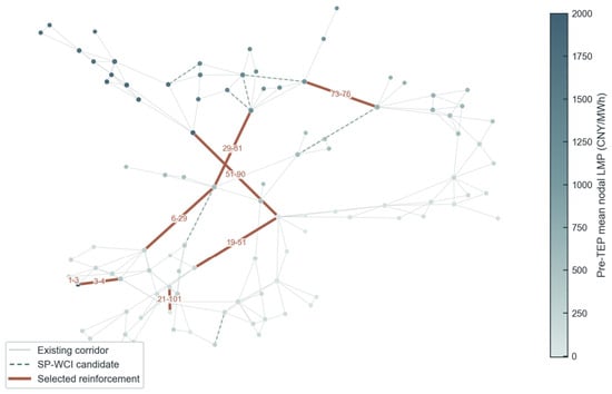
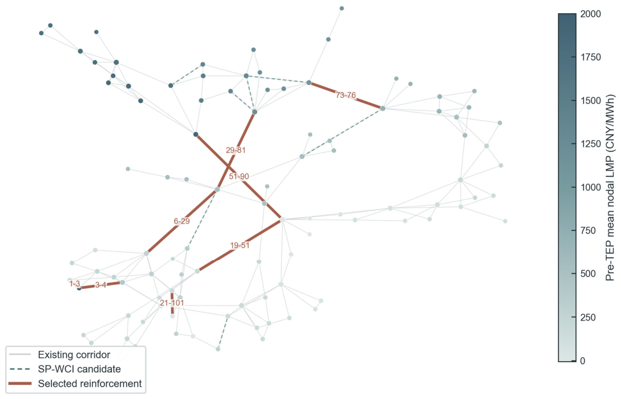
The test system is a 101-bus reduced model derived from an anonymized 796-bus grid in Southwest China. Buses were clustered by zone, loads were aggregated, parallel corridor ratings were combined, and generator capacities were reallocated by documented type-specific factors. The reduced case contains 101 buses, 175 branches, and 18 generators (Figure 2). An aggregate audit gives zero active load preservation error and one connected component. A separate capacity-preserving validation maps all 787 source generator records to the same 101 bus clusters before comparing the full and reduced DC models over the common 24 h profile. The validation gives a production cost error of 0.08%, a total objective cost error of 15.56%, a bus hour LMP MAE of 29.66 CNY/MWh, a PTDF correlation of 0.787, and 3/10 overlap among the highest utilization corridors. The mixed errors confirm that the 101-bus case is a corridor-screening surrogate rather than a full-order network equivalent.

Figure 2. Topology and selected corridors of the 101-bus reduced model.

The reduction is intended to retain the planning interactions that matter at the inter-zone level. Preserving inter-zone corridors and their thermal limits maintains the principal transfer bottlenecks, while aggregation removes internal buses whose detailed voltage behavior is outside the DC planning scope. The reduced network is, therefore, used as a corridor-planning representation rather than as a substitute for the original network in protection, stability, or detailed AC studies. This distinction is important when interpreting the results: the case study evaluates the consistency and decision value of the computational workflow, while project-level approval would require re-expansion and verification in the full network model.

A 24 h representative day is used for planning. The load profile peaks at hour 22 and reaches its minimum at hour 5; wind and solar follow distinct hourly availability profiles. Load and generation capacities are multiplied by 0.25 and 0.35, respectively, to create a stressed but feasible planning experiment. These factors are scenario assumptions for method evaluation, not a demand forecast or a calibrated probability distribution.

The hourly chronology is retained because the timing of renewable output and load, rather than their daily totals alone, determines which corridors become congested. Solar production is concentrated in the daytime, wind has a different temporal pattern, and the load maximum occurs late in the day. The resulting net injection pattern can, therefore, produce a congestion critical hour that differs from the system peak load hour. This chronological representation is also required by SCUC, where commitment transitions and ramping constraints couple adjacent periods.

The load and capacity scaling factors define the stress level of the computational experiment and are held fixed in every screening comparison and penalty sweep case. They should be interpreted as scenario parameters rather than forecasts of a specific future year. Holding them constant isolates the effect of candidate selection and expansion decisions; otherwise, differences between methods could reflect unequal operating conditions rather than the information content of the screening metric. The qualitative conclusions are not tied to this particular stress level: the same chain is re-executed on the full-order system at four times this loading in Section 3.6.

Table 1 summarizes the system scale before and after reduction.

Table 1. System scale and capacity-preserving reduction validation audit.

Parameter	Full-Order Source	101-Bus Reduced Model
Buses	796	101
Transmission branches	1191	175
Generator records/aggregated units	787	18
Wind records/units	87	3
Solar records/units	270	4
Hydro records/units	236	4
Thermal records/units	176	6
Other records/units	18	1
Peak active load (MW)	88,909.41	88,909.41
Peak load preservation error	Reference	0.00%
Connected components	—	1
Validation generator records	787	787
Production cost error	Reference	0.08%
Total objective cost error	Reference	15.56%
Bus hour LMP MAE	Reference	29.66 CNY/MWh
PTDF correlation/NRMSE	Reference	0.787/0.609
Corridor flow NMAE	Reference	100.6%
Top 10 congestion overlap	Reference	3/10

The 18 generators are categorized by type: 3 wind, 4 solar, 4 hydro, 6 thermal, and 1 other. Table 2 lists the marginal cost parameters used in this study.

Table 2. Generator marginal cost parameters.

Type	Count	c1 (CNY/MWh)	c0 (CNY/h)	Availability/Operating Setting
Wind	3	0	0	Hourly wind profile; P_min = 0
Solar	4	0	0	Hourly solar profile; P_min = 0
Hydro	4	80	0	0.98 P_max availability; P_min = 0
Thermal	6	300	80	Data P_min; ramp = 0.22 P_max/h
Other	1	250	0	Data P_min and P_max

Load shedding and renewable curtailment use separate variables and separate penalties. The main case load-shedding penalty is 2000 CNY/MWh, whereas the base curtailment penalty is 80 CNY/MWh, and the policy weight $\gamma$ is varied independently. A 1200–5000 CNY/MWh sensitivity range is evaluated for the fixed recommended topology; therefore, conclusions are not inferred from a single undocumented penalty value.

The load-shedding variable preserves feasibility at demand buses, while renewable curtailment $Q_{r,t}$ is defined only for wind, solar, and hydro units through Equation (5). For hydro, $Q_{r,t}$ represents unused hourly availability under the representative profile because an intertemporal water balance model is outside the present scope. No generic nodal dump variable is used.

2.2. SP-WCI Candidate Generation

The first stage computes an hourly shadow price-weighted congestion index for every existing transmission line $k$ and hour $t$:

$${\sigma }_{k,t}=\left|F_{k,t}\right|\left|{\lambda }_{f\left(k\right),t}-{\lambda }_{t\left(k\right),t}\right|$$

(1)

The two factors are the absolute branch flow $F_{k,t}$ and the absolute LMP difference between ${\lambda }_{f\left(k\right),t}$ and ${\lambda }_{t\left(k\right),t}$. Both are obtained from the hourly DC-OPF:

$$\underset{P_t,S_t,Q_t}{\min }{c}^T{P}_t+M_s{\sum }_n{S}_{n,t}+c^{curt}{\sum }_{r\in G_{res}}{Q}_{r,t}$$

(2)

subject to:

$$C_l^T{f}_t=C_g{p}_t-P_{d,t}+S_t,dual:{\lambda }_t$$

(3)

$$f_{k,t}=B_{k\left[{\theta }_{f\left(k\right),t}-{\theta }_{t\left(k\right),t}\right]},-L_k\le f_{k,t}\le L_k,\forall k\in E,t$$

(4)

$$0\le S_{n,t}\le P_{d,n,t},p_{r,t}+Q_{r,t}=P_{r,t}^{avail},Q_{r,t}\ge 0$$

(5)

$$P_i^{\min }\le p_{i,t}\le P_i^{\max },\forall i,t$$

(6)

The dual vector ${\lambda }_t$ of the nodal power balance constraint gives the hourly LMPs. The critical hour is retained as a diagnostic marker and is defined by the maximum total congestion surplus:

$$t^{*}=\arg \underset{t}{\max }C{S}_t,C{S}_t={\sum }_{k\in E}{\sigma }_{k,t}$$

(7)

The critical hour $t^{*}$ identifies the most economically congested operating point, but it does not by itself determine the candidate list. Greenfield cross-region corridors are appended after the existing corridor screening step so that TEP can also test reinforcements absent from the original topology.

The DC-OPF is solved for all 24 h. Hourly congestion surplus is normalized to define a nonnegative weight, and the weights sum to one:

$${\omega }_t={\displaystyle \frac{C{S}_t}{{\sum }_{\tau =1}^{24}C{S}_{\tau }}},{\sum }_{t=1}^{24}{\omega }_t=1$$

(8)

The daily screening score of line $k$ is the congestion surplus-weighted aggregate of its 24 hourly indices:

$${\overline{\sigma }}_k={\sum }_{t=1}^{24}{\omega }_t{\sigma }_{k,t}$$

(9)

Existing corridors are sorted in descending order of the aggregate score ${\overline{\sigma }}_k$ in Equation (9), and the highest-ranked $N=15$ corridors form the common candidate budget. Each candidate represents a parallel reinforcement of an observed corridor. The same budget is used for weighted overload, rule-based, and random screening.

SP-WCI has a direct congestion-rent interpretation. With flow measured in MW and the LMP difference in CNY/MWh, their product represents an hourly economic exposure associated with transferring power across the corridor. The absolute value is used for ranking because the planning question concerns the magnitude of congestion, while the sign and direction of flow remain available for engineering interpretation. A high score, therefore, requires both material utilization and material price separation; neither signal can dominate when the other is close to zero.

Congestion surplus weighting emphasizes economically consequential hours without discarding seasonal profile chronology within the representative day. The same weighting generates both the reported ranking and the optimization candidate list. The complete screening procedure is summarized in Algorithm 1.

Algorithm 1. SP-WCI-guided candidate generation

Step 1: For each hour t = 1, …, 24 of the representative day, solve the hourly DC-OPF in Equations (2)–(6); record the branch flows, the nodal LMPs obtained as duals of the nodal balance constraints, and the system-wide congestion surplus. Step 2: For every existing corridor k and hour t, compute the hourly index of Equation (1) as the product of the absolute branch flow and the absolute endpoint LMP difference. Step 3: Normalize the 24 hourly surpluses into weights by Equation (8) and aggregate the hourly indices into the corridor score by Equation (9). Step 4: Sort the 175 corridors by descending score and retain the top 15 as the candidate budget. Step 5: Append each retained candidate to the TEP model of Section 2.3 as a parallel circuit with its investment cost; enforce the same candidate budget for the weighted overload, rule-based, and random controls of Section 3.2.

2.3. Bi-Objective TEP Formulation

The TEP model minimizes the sum of annualized investment cost, daily operational cost (multiplied by 365 for annualization), and a renewable curtailment penalty:

$$\begin{array}{l}\underset{x,P,S,Q}{\min }Z=\sum _{l\in C}{c}_l^{\mathrm{inv}}a{x}_l+\\ 365{\displaystyle \sum _{t=1}^{24}}\left[c^T{P}_t+M_s\sum _n{S}_{n,t}+\left(c^{\mathrm{curt}}+\gamma \right)\sum _{r\in G_{\mathrm{res}}}{Q}_{r,t}\right]\end{array}$$

(10)

Here, $x_l$ is the binary investment decision, $a$ is the annuity factor computed with $r=0.08$ and $n=20$ years, $S$ is involuntary load shedding, $Q$ is renewable or hydro curtailment, and $\gamma$ is the curtailment policy weight. Capital and operating terms are, therefore, expressed on the same annual basis.

The objective places costs with different time bases on a common annual basis. Candidate line capital expenditure is converted through the annuity factor, while the operating cost of the representative day is multiplied by 365. The curtailment term is controlled by $\gamma$ and acts as a policy preference rather than a physical constraint: increasing $\gamma$ changes the relative value assigned to renewable accommodation without changing the network, generator, or demand data. This separation allows the same model to reveal how policy emphasis changes the selected topology.

The hourly nodal power balance is

$$C_l^T{F}_t=C_g{P}_t-P_{d,t}+S_t,\forall t$$

(11)

Existing corridors obey the DC flow relation and their thermal ratings:

$$F_{k,t}=B_{k\left[{\theta }_{f\left(k\right),t}-{\theta }_{t\left(k\right),t}\right]},-L_k\le F_{k,t}\le L_k,\forall k\in E,t$$

(12)

For each candidate corridor, the Big-M disjunction activates the DC flow relation only when the line is built:

$$-M_{k\left(1-x_k\right)}\le F_{k,t}-B_{k\left[{\theta }_{f\left(k\right),t}-{\theta }_{t\left(k\right),t}\right]}\le M_{k\left(1-x_k\right)},\forall k\in C,t$$

(13)

The candidate line rating is coupled to the same binary decision:

$$-L_k{x}_k\le F_{k,t}\le L_k{x}_k,x_k\in \left\{0,1\right\},\forall k\in C,t$$

(14)

Generator output and involuntary shedding are bounded by

$$P_i^{\min }\le P_{i,t}\le P_i^{\max },0\le S_{n,t}\le P_{d,n,t},\forall i,n,t$$

(15)

Renewable dispatch and curtailment are linked explicitly at each renewable or hydro unit:

$$P_{r,t}+Q_{r,t}=P_{r,t}^{avail},P_{r,t}\ge 0,Q_{r,t}\ge 0,\forall r\in G_{res},t$$

(16)

For candidate line $k$, $M_k$ = 2 $L_k$ + 10,000 relaxes Equation (13) when $x_k$ = 0, whereas Equation (14) forces its flow to zero. Existing corridors use Equation (12) directly. The constant is deliberately small for a disjunctive formulation. When the line is built, Equation (13) reduces to the exact DC flow relation and the value of the constant is irrelevant; when the line is not built, Equation (14) already forces its flow to zero, so the constant only needs to upper-bound the pre-construction DC flow on the corridor over all feasible phase angle differences, which is of the order of the corridor rating. The chosen value—twice the candidate rating plus a 10,000 MW margin—satisfies this requirement with a wide margin, and all reported solutions converge within the 0.5% MIP gap, indicating that the disjunction does not impair numerical solution quality.

By sweeping $\gamma$ over the set {0, 20, 50, 100, 150, 200, 300, 500, 800}, a Pareto front of investment cost versus renewable curtailment is generated. Each point on the Pareto front corresponds to a different trade-off between capital expenditure and renewable accommodation.

Because line decisions are binary, the resulting trade-off is expected to be piecewise and discontinuous rather than a smooth convex curve. Several neighboring $\gamma$ values may select the same topology, followed by a sudden jump when the reduction in penalized curtailment is large enough to justify an additional corridor. The relevant decision output is, therefore, not only the lowest objective value for a single $\gamma$ but also the set of stable topology regimes, dominated solutions, and transition points revealed by the sweep.

For interpretation, investment and curtailment are reported separately even though both enter the scalarized objective. A planning scheme is attractive when it achieves a large movement in operational outcomes before the next discrete investment jump. This knee-point logic is used in Section 3.7 to recommend a plan; it avoids presenting the penalty coefficient itself as a universal engineering constant.

2.4. SCUC–SCED and LMP Calculation

After TEP selects the optimal line set $x^{*}$, the framework performs security-constrained unit commitment (SCUC) and security-constrained economic dispatch (SCED) to evaluate the post-planning operational outcomes.

The two operational layers play different roles. SCUC captures the intertemporal and discrete feasibility of operating the selected network, including the availability of thermal units and their ramping limits. SCED then evaluates the short-run marginal cost of serving an additional unit of demand for the fixed commitment pattern. This separation is necessary because an MILP containing binary commitment variables does not provide economically interpretable nodal dual variables in the same way as a continuous dispatch problem.

For the topology selected by TEP, SCUC minimizes energy, no-load, startup, shutdown, shedding, and curtailment costs over the complete 24 h horizon:

$$\begin{array}{c}{\displaystyle \underset{P,u,v,z,S,Q}{\min }}{\displaystyle \sum _{t=1}^{24}}\left\{\begin{array}{c}\sum _{i\in G_{\mathrm{th}}}\left[c_i{P}_{i,t}+c_i^0{u}_{i,t}+c_i^{\mathrm{su}}{v}_{i,t}+c_i^{\mathrm{sd}}{z}_{i,t}\right]+\\ M_s\sum _n{S}_{n,t}+\gamma \sum _{r\in G_{\mathrm{res}}}{Q}_{r,t}\end{array}\right\}\end{array}$$

(17)

Commitment-dependent generation limits are

$$u_{i,t}{P}_i^{\min }\le P_{i,t}\le u_{i,t}{P}_i^{\max },u_{i,t}\in \left\{0,1\right\},\forall i\in G_{\mathrm{th}},t$$

(18)

Startup and shutdown allowances are included in the inter-hour ramp constraints:

$$-R_i^{down}{u}_{i,t}-P_i^{\max z_{i,t}}\le P_{i,t}-P_{i,t-1}\le R_i^{up}{u}_{i,t-1}+P_i^{\max v_{i,t}}$$

(19)

The startup variable v and shutdown variable z satisfy the commitment transition

$$u_{i,t}-u_{i,t-1}=v_{i,t}-z_{i,t},v_{i,t},z_{i,t}\in \left\{0,1\right\}$$

(20)

Minimum up- and down-time requirements are enforced by

$${\displaystyle \sum _{\tau =t}^{t+T_i^{\mathrm{up}}-1}}{u}_{i,\tau }\ge T_i^{\mathrm{up}}{v}_{i,t},\forall i,t$$

(21)

$${\displaystyle \sum _{\tau =t}^{t+T_i^{\mathrm{down}}-1}}\left[1-u_{i,\tau }\right]\ge T_i^{\mathrm{down}}{z}_{i,t},\forall i,t$$

(22)

The available committed headroom must also cover the hourly spinning reserve requirement:

$$\sum _{i\in G_{\mathrm{th}}}\left[u_{i,t}{P}_i^{\max }-P_{i,t}\right]\ge R_t,\forall t$$

(23)

With $x^{*}$ fixed by TEP (and $x_k^{*}$ = 1 for every existing branch), SCUC and SCED use

$$F_{k,t}=B_{k\left[{\theta }_{f\left(k\right),t}-{\theta }_{t\left(k\right),t}\right]},-L_{k{x}_k^{*}}\le F_{k,t}\le L_{k{x}_k^{*}},{\theta }_{ref,t}=0$$

(24)

SCED fixes the commitment schedule $u^{*}$ and the selected topology $x^{*}$ and solves the continuous dispatch problem

$$\underset{P,S,Q,F,\theta }{\min }{\displaystyle \sum _{t=1}^{24}}[c^T{P}_t+M_s\sum _n{S}_{n,t}+\gamma \sum _{r\in G_{\mathrm{res}}}{Q}_{r,t}],u=u^{*},x=x^{*}$$

(25)

Its nodal balance equation, together with Equations (15), (16), (19), (23), and (24), defines a physically feasible fixed-commitment LP:

$$C_l^T{F}_t=C_g{P}_t-P_{d,t}+S_t,dual:{\lambda }_t^{post}$$

(26)

The post-expansion LMP is the sensitivity of the optimal SCED cost to nodal demand:

$${\lambda }_{n,t}^{post}={\displaystyle \frac{\partial Z_{SCED}^{*}}{\partial P_{d,n,t}}}=dual\left[balanc{e}_{n,t}\right]$$

(27)

Hourly congestion surplus is evaluated with the same orientation-independent branch metric used in screening:

$${\mathrm{CS}}_t=\sum _{k\in E\cup C}|F_{k,t}|\left|{\lambda }_{f\left(k\right),t}-{\lambda }_{t\left(k\right),t}\right|$$

(28)

Pre-expansion values are obtained with the same SCUC-SCED formulation and no candidate lines. All generator data, profiles, penalty coefficients, reserve requirements, and solver settings remain unchanged, so the paired comparison isolates the selected topology.

This paired evaluation creates a controlled counterfactual. Generator data, hourly profiles, penalty coefficients, and solver settings are unchanged; only the candidate line investment vector differs. Consequently, changes in dispatch, LMP, shedding, and curtailment can be attributed to the expanded transfer capability under the adopted DC and representative day assumptions.

2.5. LVEI Post-Evaluation

For each selected candidate line $l$ in the optimal solution $x^{*}$, the line value evaluation index is computed as:

$$LVE{I}_l={\displaystyle \frac{\Delta C{S}_l-C_{inv,l}^{ann}}{C_{inv,l}^{ann}}}$$

(29)

Here, $\Delta {\mathrm{CS}}_l$ is the increase in annual congestion surplus when line $l$ is removed while all other selected lines remain in service, and $C_{\mathrm{inv},l}^{\mathrm{ann}}$ is its annualized cost. Under this definition, ${\mathrm{LVEI}}_l=0$ is the break-even point; positive values indicate that the conditional congestion relief value exceeds annualized cost. LVEI is a topology-dependent diagnostic and is not reported as a general project ROI.

The removal experiment is performed conditionally on all other selected lines remaining in service. LVEI is, therefore, a marginal, topology-dependent diagnostic rather than an intrinsic property of a corridor. Two lines can be substitutes, so removing either one from the complete plan may have a small effect; they can also be complements, so the value of one line may depend on the presence of another. The index should be read as evidence about the selected portfolio, not as a standalone market valuation independent of network context.

A negative LVEI does not automatically prove that a line is technically unnecessary. It indicates that, under the adopted operating profile and congestion surplus valuation, the re-dispatched system performs better on that specific economic metric when the line is removed. Such a result is a trigger for additional examination of flow redistribution, contingency benefit, voltage support, construction sequencing, and alternative routing. This diagnostic role is central to the proposed closed loop: post-evaluation can refine the candidate pool or motivate a new planning run instead of being treated as a final ranking only.

2.6. Computational Implementation

The framework is implemented in MATLAB R2022a with MATPOWER, YALMIP, and Gurobi [24,25,26]. DC-OPF and SCED are linear programs; TEP and SCUC are mixed-integer linear programs. The relative MIP gap is 0.5% for every method. All comparisons retain the same 24 h profile, 15-corridor candidate budget, cost parameters, and solver tolerance. Random screening is repeated for ten independent seeds and summarized by its mean, standard deviation, and 95% confidence interval. On a standard workstation, one 24 h DC-OPF screening pass over all 175 corridors takes 10.4 s, the 15-candidate TEP MILP solves in 12.0 s, and one complete SCUC–SCED verification of a fixed topology takes 18.2 s. On the full-order 796-bus system, the screening pass requires 24 hourly LP solves of a few seconds each and the 15-candidate TEP MILP solves in 1.6 s (Section 3.6).

The computational experiment is organized so that each method changes only the candidate-screening rule. All four methods receive the same candidate count, solve the same TEP formulation, and are evaluated through the same SCUC–SCED pipeline. This design mirrors a controlled model comparison study: an improvement is credited to the screening signal only when it persists under a common optimization budget and common downstream evaluation. The $\gamma$ sweep is likewise warm-start independent in interpretation; repeated topology selections are reported as stable regimes rather than counted as distinct planning solutions.

Reproducibility also depends on retaining the intermediate outputs that connect stages. The hourly DC-OPF results determine the candidate ranking, the TEP investment vector fixes the operational topology, the SCED dual variables determine the LMP and congestion surplus metrics, and the line removal runs determine LVEI. Reporting these links makes it possible to audit whether a surprising result originates in screening, investment selection, dispatch, or post-evaluation rather than treating the workflow as a single opaque solver call.

3. Computational Results and Validation

The validation follows the same order as the computational framework. Candidate-ranking results first establish what SP-WCI detects and when the critical condition occurs. A controlled comparison then tests whether that information produces a more efficient expansion portfolio than three alternative screening rules. The $\gamma$ sweep evaluates decision sensitivity, SCUC–SCED results quantify operational improvement, and the final leave-one-line-out experiment tests whether system-level benefits are distributed consistently across the selected corridors. This ordering separates observations, comparative evidence, and diagnostic interpretation. Finally, an investment effectiveness comparison and a bus hour LMP map provide two standalone views of portfolio efficiency and the spatial distribution of operating benefits.

3.1. SP-WCI Candidate Ranking

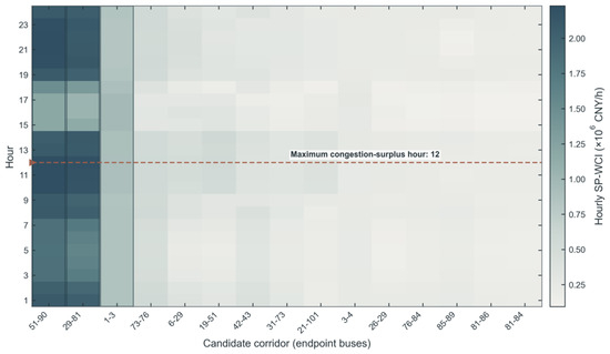
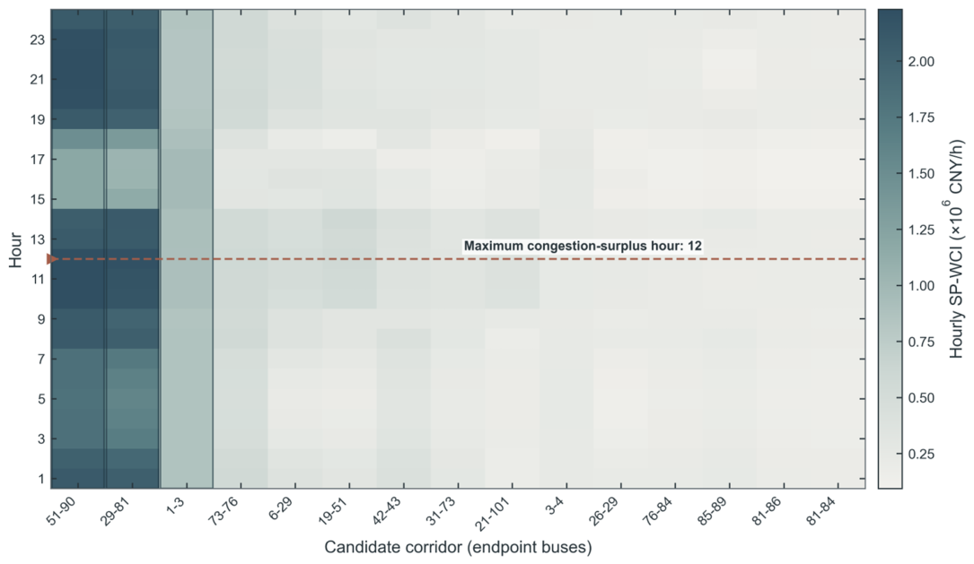
Figure 3 shows the weighted SP-WCI candidate set across all 24 h. The horizontal axis contains exactly the 15 corridors passed to TEP, and hour 12 is marked because it has the largest pre-expansion congestion surplus. The three highest daily weighted scores occur on 51–90, 29–81, and 1–3. Their intensities vary across hours, confirming that the candidate pool is supported by a multi-period signal rather than a single snapshot.

Figure 3. Twenty-four-hour SP-WCI heatmap for 15 candidate corridors.

Only 15 entries appear on the horizontal axis because the heatmap visualizes the screened candidate pool passed to the TEP model rather than all 175 original branches. Replacing ordinal indices 1–15 with the actual endpoint bus pairs makes the physical identity of each candidate explicit.

The SP-WCI ranking identifies lines that are not necessarily the most physically loaded. For example, lines 1–3 carry only 63% of their thermal limit at t* but rank second in SP-WCI because their LMP differential exceeds 200 CNY/MWh—reflecting the economic rather than purely physical nature of the index. This demonstrates the ability of SP-WCI to capture latent congestion missed by traditional overload-based methods.

The timing of the critical condition is itself informative. The maximum SP-WCI condition occurs at hour 12, whereas the load coefficient reaches its maximum at hour 22. Thus, the most economically congested condition is not simply the highest-demand condition. It reflects the spatial coincidence of renewable injections, transfer limits, and nodal demand. This distinction supports chronological OPF screening instead of selecting one conventional peak load snapshot.

The heatmap also separates persistent from event-specific candidates. A corridor with elevated values over many hours represents a recurring transfer limitation, while a narrow high-value band indicates sensitivity to a particular injection pattern. Both can be relevant to planning, but they imply different follow-up checks: persistent congestion supports structural reinforcement, whereas event-specific congestion may also be addressed through operating measures, storage, or generation redispatch. SP-WCI provides this temporal diagnostic before the investment model is solved.

3.2. Comparative Validation of Candidate Screening Methods

Table 3 compares SP-WCI, weighted overload, rule-based, and random screening under the same candidate budget and the automatically selected $\gamma =0$. The random entry is the mean of ten seeds, with 95% confidence intervals reported in the table. All four methods solve the identical TEP formulation with the same objective coefficients, candidate budget, solver settings, and 0.5% MIP gap; only the candidate sets differ, so performance differences are attributable to the screening signal alone. The rule-based heuristic generates its candidate set algorithmically: each existing corridor is scored by a dominant term that flags voltage-level mismatch between its two terminal buses, plus a secondary term equal to the normalized series impedance (r² + x²) of the corridor, and the 15 highest-scoring corridors are retained; no expert panel or elicitation protocol is involved.

Table 3. Comparison of candidate selection methods ($\gamma =0$, 15 candidates each).

Method	Lines	Investment (Million CNY)	Pre-LMP (CNY/MWh)	Post-LMP (CNY/MWh)	LMP Red. (%)	Shedding (MWh)	Efficiency (% Red. Per Million CNY)
SP-WCI	8	24.0	597.33	259.98	56.5	0.0	2.35
Weighted overload	13	39.0	597.33	255.28	57.3	256.6	1.47
Rule-based heuristic	5	15.0	597.33	374.48	37.3	10,090.2	2.49
Random (10 seeds)	6.9 ± 1.3	20.7 ± 3.8	597.33	549.51 ± 40.10	8.0 ± 6.7	17,154.7 ± 1708.3	0.39

SP-WCI selects eight circuits with an investment of 24.0 million CNY and an average LMP reduction of 56.5%. Weighted overload screening gives 57.3% using 13 circuits, while the rule-based heuristic gives 37.3%. The ten-seed random benchmark averages 8.0% (95% CI ± 6.7 percentage points). These results compare screening strategies; they do not identify engineering constructability or causal project returns. Weighted overload attains a marginally larger absolute LMP reduction (57.3% versus 56.5%), but it requires 13 circuits and 39.0 million CNY—62.5% more investment—and still leaves 256.6 MWh of load unserved. Normalized by investment (Table 3, last column), SP-WCI achieves 2.35 percentage points of LMP reduction per million CNY versus 1.47 for weighted overload, and its plan is the only one that fully eliminates load shedding. The rule-based heuristic shows a higher raw ratio (2.49) only because it purchases a much smaller absolute reduction (37.3%) at low cost while leaving 10,090.2 MWh unserved, so the efficiency ratio must be read jointly with adequacy. We, therefore, claim superior investment efficiency and adequacy of the SP-WCI candidate set, not the largest absolute LMP reduction.

The comparison is evaluated jointly through investment, LMP, unserved energy, and unused renewable/hydro availability. Because the pre-expansion case is intentionally stressed, the absolute shedding values should not be interpreted as a reliability forecast. The relevant result is whether rankings remain favorable under the same operational model and candidate budget.

This experiment does not imply that engineering judgement or loading information is dispensable. Expert review remains necessary for constructability, voltage level, right of way, and protection requirements, while loading ratios remain useful for asset security assessment. The result instead clarifies their role: they are stronger as feasibility and review filters around an economically informed candidate generator than as the sole ranking criterion for a market-oriented TEP problem.

3.3. Weighting Scheme Ablation for the SP-WCI Ranking

A natural question concerning the SP-WCI screening stage is how much of its performance stems from the congestion surplus weighting in Equations (8) and (9), and how much from the underlying flow–price difference product itself. We, therefore, recomputed the corridor ranking under four hourly weighting schemes: (i) the baseline congestion surplus weighting; (ii) an equal-weighted 24 h average; (iii) a critical hour-only scheme retaining only the hour with the highest congestion surplus (hour 12); and (iv) an adversarial control that weights only low-congestion hours (below 75% of the daily peak). The studied representative day is heavily stressed: the hourly congestion surplus remains between 7.2 and 12.9 million CNY/h throughout the day.

The three economically reasonable schemes yield essentially the same corridor ordering over all 175 corridors (Table 4): the equal-weighted and critical-hour-only schemes both reproduce the baseline top 15 candidate set exactly, with Spearman rank correlations of 0.9999 and 0.9823, and even the adversarial weighting shares 14 of the 15 top corridors. The screening signal is thus dominated by the flow–price difference product in Equation (8), and the surplus weighting is a refinement with clear economic interpretability rather than a free parameter that drives the result.

Table 4. Corridor-ranking comparison of SP-WCI under four hourly weighting schemes.

Weighting Scheme	Hour Weights	Top 15 Overlap with Baseline	Spearman Rank Correlation (175 Corridors)
Congestion surplus weighting (baseline, Equations (8) and (9))	proportional to hourly congestion surplus	–(reference)	–(reference)
Equal-weighted 24 h average	1/24 for all hours	15/15	0.9999
Critical hour only (hour 12)	unit weight on the peak surplus hour	15/15	0.9823
Low-congestion hours (adversarial)	uniform over hours with surplus < 75% of peak	14/15	–

At the plan level (Table 5), the equal-weighted scheme produces the identical expansion plan as the baseline (eight circuits, 24.0 million CNY, average LMP reduction of 56.5%). The adversarial scheme, despite differing in only one candidate corridor, leads to a noticeably less efficient plan (nine circuits, 27.0 million CNY; normalized efficiency 2.10 versus 2.35). The SP-WCI ranking is, therefore, robust to the choice among economically reasonable hour-weighting schemes, while the congestion surplus weighting safeguards investment efficiency by directing the screening toward the hours in which congestion rents actually accrue.

Table 5. Plan-level outcomes of the weighting scheme ablation (γ = 0, budget = 15).

Weighting Scheme	Selected Lines	Investment (Million CNY)	Post-LMP (CNY/MWh)	LMP Reduction (%)	Unused Availability (MWh)	Efficiency (% Red. Per Million CNY)
Surplus-weighted (baseline)	8	24.0	259.98	56.5	50,398.7	2.35
Equal-weighted 24 h average	identical candidate set and plan as baseline	–	–	–	–	–
Low-congestion hours (adversarial)	9	27.0	258.04	56.8	39,537.0	2.10

3.4. Sensitivity of the Recommended Topology to the Candidate Budget

The candidate budget was fixed at 15 corridors in the main study. To demonstrate that the recommended topology is not an artifact of this choice, we repeated the screening–optimization–verification chain with budgets of 10 and 20 corridors, keeping all other settings unchanged (γ = 0, identical formulation and solver). The results are summarized in Table 6.

Table 6. Candidate budget sensitivity of the recommended expansion plan (γ = 0).

Candidate Budget	Selected Lines	Investment (Million CNY)	Post-LMP (CNY/MWh)	LMP Reduction (%)	Unused Availability (MWh)	Efficiency (% Red. Per Million CNY)	Core Topology Preserved
10	8 (identical plan)	24.0	259.98	56.5	50,398.7	2.35	Yes
15 (baseline)	8	24.0	259.98	56.5	50,398.7	2.35	Yes
20	14	42.0	261.86	56.2	16,333.9	1.34	Yes (6/6 core corridors)

With the budget of 10 corridors, the optimization returns exactly the same eight-circuit plan as the baseline. With the budget of 20 corridors, the six highest-ranked corridors of the recommended plan are again selected, and the resulting 14-circuit plan costs 42.0 million CNY, achieves essentially the same LMP reduction (56.2%), and lowers the unused renewable/hydro availability from 50.4 to 16.3 GWh per day; the normalized efficiency declines from 2.35 to 1.34 percentage points per million CNY, showing clear diminishing marginal returns.

Overall, the recommended topology is robust rather than an artifact of the chosen budget: the core corridors are invariant across budgets of 10–20 corridors, and a budget of 15 places the plan at the knee between investment efficiency and renewable energy utilization (Table 6).

3.5. Robustness of the Recommended Topology Across Representative Days

The main study optimizes the expansion plan for a single representative 24 h profile. To test whether the recommended topology is tied to this particular profile, we repeated the complete chain on three additional representative days that stress the system in different directions, a high-load day (loads ×1.10), a high-renewable day (wind and solar availability ×1.15), and a low-renewable day (×0.85), with all other settings identical to the main study (Table 7).

Table 7. Robustness of the recommended expansion plan across four representative days (γ = 0).

Representative Day	Load ×/Renew. ×	Baseline Top 15 Re-Identified	Selected Circuits (Investment, 104 CNY)	Recommended 8 Circuits Reproduced	LMP Pre → Post (CNY/MWh)	Shedding Pre → Post (MWh)	Unused RE/Hydro Pre → Post (MWh)
D1 (baseline)	1.00/1.00	—	8 (2400)	8/8	597.33 → 259.98	21,159.0 → 0.0	117,883.0 → 50,398.7
D2 (high load)	1.10/1.00	12/15	11 (3300)	7/8	669.94 → 266.73	35,298.8 → 176.5	108,696.9 → 12,143.1
D3 (high renewable)	1.00/1.15	15/15	8 (2400)	8/8	594.00 → 258.74	21,045.6 → 0.0	128,251.4 → 57,734.8
D4 (low renewable)	1.00/0.85	14/15	10 (3000)	7/8	600.09 → 271.54	21,337.1 → 0.0	107,367.3 → 33,359.7

The recommended topology is stable across all four days: six of the eight recommended circuits are selected on every day, the high-renewable day reproduces the exact eight-circuit plan of the main study, and 12 to 15 of the 15 baseline candidate corridors are re-identified in every scenario; day-specific adjustments concern only marginal circuits. The expansion eliminates load shedding on three of the four days—on the high-load day, a residual of 176.5 MWh/day (0.5% of the pre-expansion value) remains economically optimal at VOLL = 2000 CNY/MWh—keeps the post-expansion average LMP at 258.7–271.5 CNY/MWh in all cases and reduces the unused renewable/hydro availability by 55.0–88.8%. The recommended corridors, therefore, reflect structural transfer bottlenecks rather than a particular daily profile.

3.6. Native Validation on the Full-Order 796-Bus System

The 101-bus equivalent network used in Section 3.1, Section 3.2, Section 3.3, Section 3.4 and Section 3.5 is a screening surrogate: it preserves the zonal structure and the main transfer paths of the Yunnan grid, but it does not necessarily reproduce corridor-level congestion signals of the full-order system. To establish that the proposed framework itself is not tied to the reduced model, we re-ran the complete chain natively on the full-order model (796 buses, 787 generators, 1191 in-service branches aggregated into 175 inter-zonal corridors under the same partition). Load and generation were scaled by a factor of four to obtain a stressed planning scenario; all other settings are identical to the main study. In this state, the full-order system exhibits a daily congestion surplus of 33.19 million CNY and 825.4 MWh/day of involuntary load shedding.

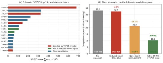
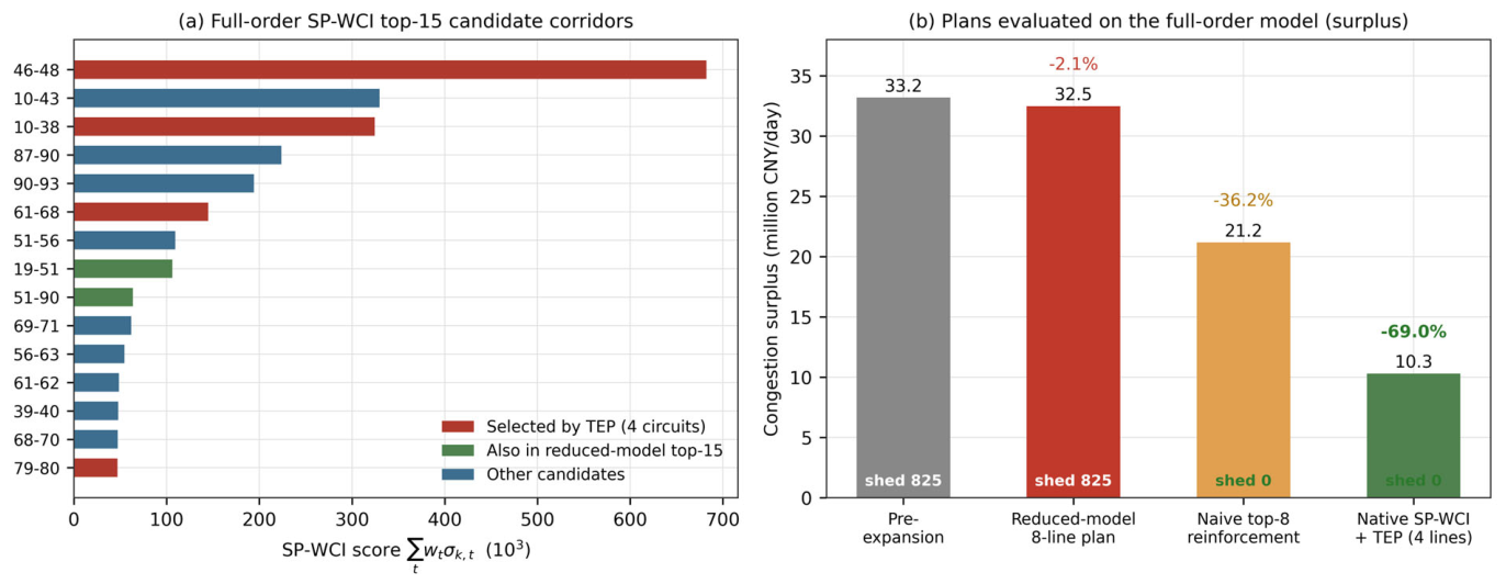
The full-order SP-WCI ranking (Figure 4a) differs markedly from the reduced model ranking: only two corridors (19–51 and 51–90) appear in both top 15 lists, and the Spearman rank correlation between the reduced and full-order corridor scores is merely 0.09. We report this gap deliberately: it confirms that the reduced model must not be used to nominate specific corridors for the real system, and it shows that neither the screening nor the investment optimization stage depends on any particular network reduction—both can be executed directly on the full-order model at negligible computational cost.

Figure 4. Full-order validation: (a) SP-WCI top 15 corridors; (b) surplus of four plans.

With the 15 full-order candidates, the investment optimization of Section 2.3 is solved by Gurobi in 1.6 s and selects only four circuits (46–48, 10–38, 61–68, and 79–80) for a total investment of 12.0 million CNY. Notably, the optimizer discards the second-ranked corridor 10–43 and instead selects the 15th-ranked corridor 79–80, illustrating that system-wide congestion relief is driven by the portfolio effect of the selected circuits rather than by individual screening scores.

Table 8 and Figure 4b compare four plans, all evaluated on the full-order model: (i) the pre-expansion reference; (ii) the eight-circuit plan recommended in Section 3.7 mapped onto the corresponding full-order corridors, which reduces the congestion surplus by only 2.1% and leaves load shedding unchanged at 825.4 MWh/day; (iii) naive doubling of the eight highest-scoring full-order corridors at the same 24.0 million CNY cost, which reduces the surplus by 36.2% and eliminates load shedding; and (iv) the native SP-WCI + TEP plan, which reduces the surplus by 69.0%—almost twice the relief of plan (iii)—at only half of its investment (12.0 million CNY), eliminates load shedding, and decreases the daily production cost by 1.2%. A plan that is optimal on the surrogate, therefore, does not transfer to the full-order system, whereas the native chain does. Production cost was not recorded for the naive plan.

Table 8. Four-way comparison on the full-order 796-bus model (4× loading).

Metric	Pre-Expansion	Reduced Model Plan (8 Circuits)	Naive Top 8 Reinforcement	Native SP-WCI + TEP (4 Circuits)
New circuits	–	8	8	4
Investment (million CNY)	–	24.0	24.0	12.0
Congestion surplus (million CNY/day)	33.19	32.48 (−2.1%)	21.17 (−36.2%)	10.30 (−69.0%)
Load shedding (MWh/day)	825.4	825.4	0	0
Unused renewable/hydro energy (GWh/day)	1594.9	1594.9	1588.2	1588.3
Average LMP (CNY/MWh)	4.91	4.92	−13.37	−14.81
Production cost (million CNY/day)	104.48	104.44	–	103.19

Three conclusions follow. First, the proposed framework is model-agnostic and scalable: the full-order chain requires only 24 hourly LP solves for screening plus a 15-candidate MILP that Gurobi solves in 1.6 s on a standard workstation. Second, the reduced 101-bus model is appropriate for methodological studies and rapid algorithmic comparisons, but engineering deployment should execute the full chain on the full-order model; the weak rank correlation (0.09) and the failure of the reduced model plan on the full-order system (−2.1%) define the limitation of the surrogate explicitly. Third, the value of the framework does not rest on the surrogate: even on the full-order system, shadow price-guided screening combined with investment optimization doubles the congestion relief per unit of investment relative to naive reinforcement of the most congested corridors. Constructing network equivalents with certified corridor-level congestion fidelity is left as future work.

3.7. Pareto Front: Investment vs. Curtailment Trade-Off

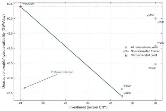
Figure 5 and Table 9 display all nine $\gamma$ outcomes and connect only the non-dominated investment–unused availability frontier. The recommended point is selected algorithmically: the investment and the unused availability of each non-dominated outcome are min–max-normalized across the non-dominated set, and the outcome minimizing the Euclidean distance to the utopia point (minimum investment, minimum unused availability) is recommended; it occurs at $\gamma =0$, with eight circuits, 24.0 million CNY of investment, and 50,398.7 MWh of unused renewable/hydro availability.

Figure 5. Investment versus unused-availability Pareto outcomes.

Table 9. Pareto front solutions for different $\gamma$ values.

γ	Lines	Investment (Million CNY)	Unused Availability (MWh)	Avg. LMP (CNY/MWh)	Shedding (MWh)
0	8	24.0	50,398.7	259.98	0.0
20	8	24.0	50,398.7	257.40	0.0
50	8	24.0	50,398.7	253.52	0.0
100	12	36.0	50,006.1	269.61	68.3
150	12	36.0	50,003.4	262.34	68.3
200	12	36.0	49,083.2	255.12	68.3
300	12	36.0	48,466.5	241.30	92.3
500	11	33.0	47,630.2	224.85	416.0
800	11	33.0	47,394.4	182.50	533.7

At $\gamma =0$, the model selects eight circuits, invests 24.0 million CNY, and leaves 50,398.7 MWh of renewable/hydro availability unused.

The normalized distance rule selects $\gamma =0$.

At $\gamma =800$, the solution contains 11 circuits, invests 33.0 million CNY, and leaves 47,394.4 MWh unused. Any dominated outcomes are shown but are not called Pareto points.

The recommended topology is the $\gamma =0$ solution selected from the non-dominated set by a transparent normalized distance rule. Because line decisions are discrete, equal or non-monotonic outcomes can occur across adjacent $\gamma$ values; the interpretation is, therefore, based on realized objective values rather than on $\gamma$ alone.

The repeated solutions across neighboring $\gamma$ values indicate that the eight-circuit topology is robust to moderate changes in the curtailment preference. The first topology transition occurs only when $\gamma$ reaches 100, where the plan expands from eight to twelve circuits, and investment rises from 24.0 to 36.0 million CNY, while the unused availability decreases by only 392.6 MWh. This incremental option may be attractive to a planner with a stronger renewable accommodation target, but it is distinct from the knee-point recommendation because it purchases the final portion of improvement at a higher marginal capital requirement.

The solution at $\gamma =300$ is dominated in the reported investment curtailment plane by the $\gamma =200$ solution: it requires more lines and more investment while producing greater curtailment. Such a point would be obscured if only the scalar objective were reported. Separating the physical outputs exposes the effect of network interactions and provides a safeguard against interpreting a higher policy penalty as automatically producing a better engineering outcome.

3.8. LMP and Congestion Surplus Improvement

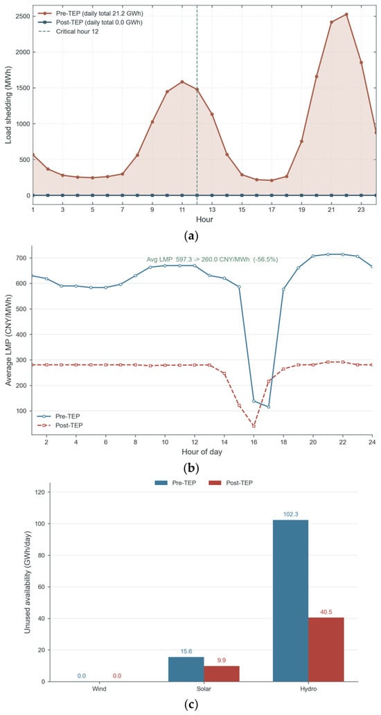
Figure 6a–c compare the pre- and post-TEP operating outcomes for the recommended $\gamma =0$ topology.

Figure 6. (a). Hourly load shedding before and after TEP. (b). Hourly average LMP before and after TEP. (c). Unused wind, solar, and hydro availability before and after TEP.

As shown in Figure 6a, the stressed pre-expansion case sheds 21,159.0 MWh (4.95% of daily demand). The recommended plan reduces this to 0.0 MWh (0.00%), a 100.0% reduction. These values measure performance in the constructed stress scenario and are not presented as an observed utility reliability level.

Figure 6b shows that the daily bus hour average LMP decreases from 597.33 to 259.98 CNY/MWh (56.5%). Hourly and nodal distributions are retained in Section 3.10 so that this average is not over-interpreted as a uniform system-wide price change.

Figure 6c reports the unused renewable and hydro availability. Values are calculated directly from the explicit curtailment variables, not hard-coded rates. Wind, solar, and hydro unused availability changes from 0.0, 15,565.8, and 102,317.2 MWh to 0.0, 9893.0, and 40,505.7 MWh, respectively. The total changes from 117,882.9 to 50,398.7 MWh (57.2%). Hydro is labeled as unused availability because no intertemporal water balance is modeled. Because no intertemporal water balance is modeled, the hydro component is an upper bound on physically lost energy: with reservoir shifting across hours, part of the unused hydro availability could be recovered later in the day. The pre-/post-comparison remains consistent because both cases share the same representation.

Dispatch changes are reported without an unsupported merit-order narrative. Wind, solar, and hydro output changes from 45,919.3, 35,476.7, and 150,455.0 MWh before expansion to 45,919.3, 41,149.5, and 212,266.4 MWh after expansion. These differences result jointly from network feasibility, commitment, ramping, availability, and the stated cost parameters; the experiment does not isolate a causal displacement mechanism.

Taken together, the three operational indicators show that the expansion plan changes both adequacy and economic dispatch. The complete elimination of load shedding (21,159.0 to 0.0 MWh) indicates that the pre-expansion network limitation was not merely a price convergence issue; it constrained the ability to serve demand. The simultaneous decline in average LMP and renewable curtailment indicates that the added transfer capability reduces expensive congestion while improving access to low-marginal-cost resources. Agreement across these metrics is stronger evidence than any single indicator in isolation.

Residual shedding remains concentrated in a limited set of daytime and evening hours, showing where the recommended plan ceases to be sufficient under the adopted scenario. These intervals are useful for the next planning iteration because they identify the operating conditions that should be examined through contingency, seasonal, or AC checks. In this way, the post-TEP operation is not only a performance report; it produces the boundary conditions for subsequent model refinement.

3.9. LVEI Line Value Evaluation

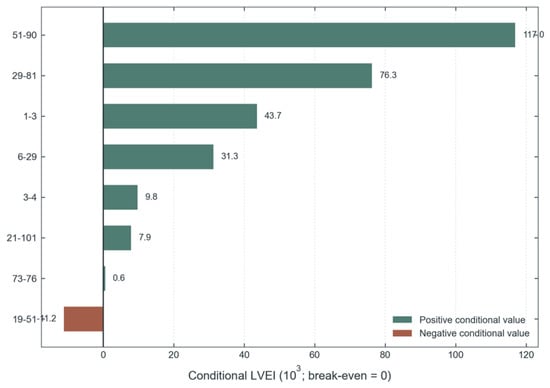
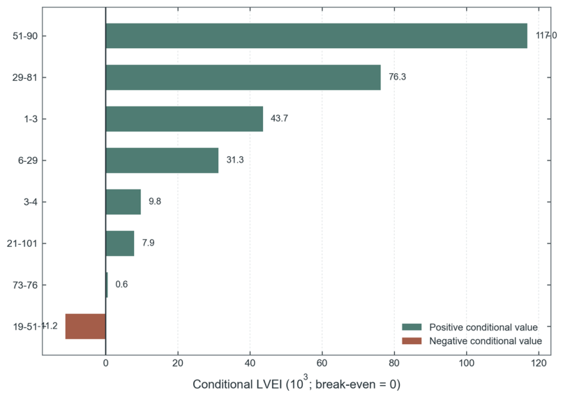
Figure 7 and Table 10 present LVEI for the eight selected circuits. The plotted break-even threshold is $\mathrm{LVEI}=0$, consistent with Equation (29). Each candidate circuit costs 3.0 million CNY; annualized at an 8% discount rate over a 20-year planning horizon (annuity factor 0.1019), this gives the 0.306 million CNY per year reported in Table 10.

Figure 7. Conditional LVEI values of the selected circuits.

Table 10. LVEI evaluation of selected transmission lines.

Rank	Line (Bus–Bus)	ΔCS_l (Million CNY/yr)	Annualized Cost (Million CNY/yr)	LVEI	Assessment
1	51–90	35,741.662	0.306	116,971.30	Positive
2	29–81	23,310.145	0.306	76,286.48	Positive
3	1–3	13,341.762	0.306	43,662.80	Positive
4	6–29	9578.702	0.306	31,347.37	Positive
5	3–4	2988.850	0.306	9780.66	Positive
6	21–101	2419.512	0.306	7917.38	Positive
7	73–76	181.038	0.306	591.49	Positive
8	19–51	−3435.302	0.306	−11,243.77	Negative

Seven of the eight selected circuits have positive conditional LVEI values, and one has a negative value. The largest value occurs on 51–90 ($\mathrm{LVEI}=116,971.3$). This identifies a strong marginal congestion relief contribution within the selected portfolio, but it is not described as a commercial rate of return.

Negative LVEI values indicate that the line removal redispatch lowers the chosen congestion surplus metric after annualized cost is considered. Such values flag topology interactions for engineering review; they do not prove that a corridor lacks reliability, voltage, contingency, or long-term option value.

The absolute magnitude of the LVEI values also warrants clarification. The numerator annualizes a daily congestion surplus change—a rent transfer between market participants rather than a welfare measure—by scaling the representative day by 365, whereas the denominator is the 0.306 million CNY annualized circuit cost. Ratios such as 116,971 for corridor 51–90, therefore, do not represent an investable return; the index is used ordinally to rank the conditional marginal contributions of the selected circuits within the evaluated portfolio.

A direct pruning test confirms this interpretation. Removing the only negative LVEI circuit (19–51) and re-running the complete SCUC–SCED verification leaves load shedding at zero and even reduces the average LMP slightly (255.66 versus 259.98 CNY/MWh), but the unused renewable/hydro availability rises from 50,398.7 to 52,420.7 MWh/day (+4.0%) and the daily production cost increases by 0.6%. The circuit is, therefore, retained: its removal improves the congestion rent metric while degrading renewable utilization and operating cost—precisely the kind of interaction that LVEI is designed to flag for engineering review rather than to resolve automatically.

The mixed LVEI signs reveal portfolio interactions. Candidate screening identifies pre-expansion bottlenecks, whereas leave-one-line-out evaluation measures a conditional post-expansion marginal effect. The two stages, therefore, answer different questions and should not be collapsed into one ranking.

For implementation, the LVEI results support a tiered review. Strongly positive corridors can proceed to detailed feasibility studies first. Negative or near-zero corridors should be tested under alternative operating profiles and with other candidate combinations before commitment. This ordering does not alter the optimized plan automatically; it directs scarce engineering analysis effort toward the investments whose system interactions are least certain.

3.10. Additional Cost-Effectiveness and Spatiotemporal Analysis

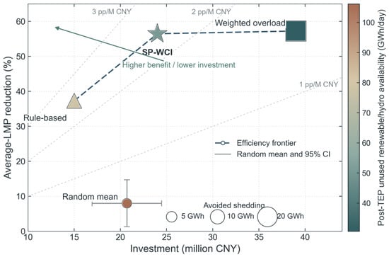
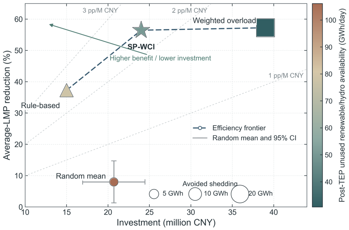
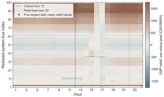
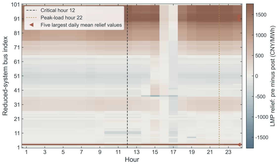
Two additional views complete the case study interpretation. Figure 8 combines investment, average LMP reduction, avoided load shedding, post-TEP unused renewable/hydro availability, and random benchmark uncertainty in one multi-criteria performance map. Figure 9 disaggregates LMP relief across all 101 buses and 24 h.

Figure 8. Multi-criteria comparison of candidate-screening methods. The dashed line connects the non-dominated methods (efficiency frontier), and the arrow indicates the preferred direction of higher benefit at lower investment.

Figure 9. Bus hour LMP relief under the recommended plan.

The preferred region in Figure 8 is the upper left. SP-WCI lies at 24.0 million CNY and 56.5% LMP reduction; weighted overload lies at 39.0 million CNY and 57.3%; and the rule-based heuristic lies at 15.0 million CNY and 37.3%. The random mean is 20.7 million CNY and 8.0%, with horizontal and vertical whiskers showing its 95% confidence intervals. The dashed method frontier and the light iso-efficiency guides make the investment effectiveness trade-off explicit without reducing the comparison to a single ratio.

Figure 9 defines LMP relief as pre-TEP minus post-TEP nodal price. The five largest daily bus average relief values occur at reduced system buses 3, 90, 91, 92, 93, ranging from 1558.12 to 1716.19 CNY/MWh. This spatial concentration is more informative than the system average change alone.

The largest bus average hourly relief occurs at hour 15 and equals 464.44 CNY/MWh. Some bus hour cells can show local price increases after redispatch even when the overall mean falls from 597.33 to 259.98 CNY/MWh; Figure 9 makes this heterogeneity explicit.

In practice, the penalty should be set from the regulator’s value of lost load or an internal reliability cost estimate and then swept rather than fixed. Post-expansion shedding is zero at every tested value, so the adequacy conclusion of the recommended topology does not depend on a particular choice within the 1200–5000 CNY/MWh band; the sweep itself, rather than any single value, is the recommended decision input.

Table 11 tests the fixed recommended topology under three load-shedding penalties. The post-expansion shedding result remains below the pre-expansion result at every tested value. This sensitivity is reported separately from commercial valuation because the penalty is a model parameter.

Table 11. Sensitivity of the fixed recommended plan to the load-shedding penalty.

Penalty (CNY/MWh)	Pre-LMP	Post-LMP	Pre Shedding (MWh)	Post Shedding (MWh)	Pre Unused (MWh)	Post Unused (MWh)
1200	419.67	259.98	27,303.9	0.0	89,809.4	50,398.7
2000	597.33	259.98	21,159.0	0.0	117,882.9	50,398.7
5000	1156.70	259.98	19,678.5	0.0	129,143.8	50,398.7

4. Discussion and Engineering Implications

The results support three levels of interpretation. The first concerns why the joint flow price signal improves candidate screening; the second concerns how discrete topology changes affect the investment curtailment trade-off; and the third concerns why an optimized portfolio can still contain lines with weak marginal value. The following discussion relates these mechanisms to practical planning decisions, while keeping the scope of the DC representative day case study explicit. As detailed in Section 3.2, the marginally higher absolute reduction in weighted overload comes with 62.5% more investment and residual unserved energy; normalized by investment, SP-WCI achieves 2.35 versus 1.47 percentage points per million CNY.

4.1. Advantages of SP-WCI over Conventional Candidate Selection

In this case, SP-WCI provides a 56.5% average LMP reduction, compared with 57.3% for weighted overload and 37.3% for the rule-based heuristic. The random mean is 8.0% (95% CI ± 6.7). The comparison is supported by a 0.5% MIP gap and repeated random trials, so small differences are not attributed to a single loose-tolerance or single-seed run.

The rule-based engineering heuristic generates its candidate set algorithmically from voltage-level mismatch and impedance criteria, without an expert panel or an elicitation protocol. The comparison in Table 3, therefore, tests a reproducible algorithmic baseline rather than subjective planner experience.

The advantage can be understood as an alignment between the screening metric and the downstream objective. The TEP and SCED stages respond to marginal production cost, unserved energy, curtailment, and network constraints. SP-WCI uses the same nodal dual information that later determines LMP outcomes, so its ranking is closer to the economic mechanism evaluated downstream. Overload rate screening would be expected to approach SP-WCI only in systems where thermal stress and price separation are strongly collinear; the present case demonstrates that this condition cannot be assumed in a renewable-rich network.

4.2. Pareto Front and Decision-Making Implications

The $\gamma$ sweep produces discrete topologies rather than a smooth curve. After dominated points are removed, the normalized distance rule recommends $\gamma =0$. The selection follows the multi-objective decision logic used in expansion planning [13,16,27].

Non-monotonic raw outcomes can arise from discrete line choices and the fact that TEP and fixed-topology SCUC–SCED are separate optimization stages. For this reason, Figure 5 connects only realized non-dominated outcomes; dominated points remain visible for audit but are not interpreted as the Pareto frontier.

For decision-making, $\gamma$ is treated as a preference parameter. Planners should compare non-dominated topologies, incremental unused availability reductions, and investment before detailed AC and contingency assessment rather than assigning policy meaning to $\gamma$ itself.

4.3. LVEI and the Case for Post-Evaluation

The LVEI analysis gives seven positive and one negative conditional values among eight selected circuits. This does not contradict portfolio optimality: the TEP solution is chosen for the complete objective, whereas LVEI changes one line at a time and measures congestion surplus after redispatch.

LVEI is, therefore, used as a second-screen diagnostic. Strong positive values prioritize detailed study, while negative or near-zero values motivate topology, scenario, and contingency review. It is not used to delete lines automatically or to claim a standalone financial return.

LVEI also helps prevent an over-interpretation of the MILP solution. An optimal binary investment vector is optimal for the complete objective and candidate set, but it does not establish a causal return for each component. The leave-one-out counterfactual supplies that missing local evidence. Its limitation is equally important: because it conditions on the remaining lines, it does not allocate the value of interactions in the manner of a full cooperative game or multi-line removal analysis. The index is best used to flag cases for review rather than to assign an immutable financial return.

4.4. Limitations

This study does not include N−1 constraints and applies a DC network model. The main results are based on one representative 24 h profile: the four-day robustness check in Section 3.5 shows that the core topology is stable under load and renewable variations, but a formal multi-scenario or stochastic formulation remains open. Moreover, the 101-bus network is a corridor-planning surrogate: as quantified in Section 3.6, its corridor-level congestion ranking does not transfer to the full-order system, and the reduced model results should be read as a computational proof of concept rather than as a deployable plan. Future extensions can add contingency-constrained planning [28,29], stochastic multi-scenario optimization [30], AC validation, and impedance margin-based stability assessment for IBR-penetrated systems [31] without changing the screening–planning–post-evaluation sequence.

4.5. Engineering and Decision Support Implications

From an engineering decision support perspective, the framework can be used as a screening and diagnostic layer around an existing planning process. SP-WCI reduces a large corridor universe to an economically informed candidate set; the $\gamma$ sweep makes the investment curtailment trade-off explicit; and LVEI flags lines requiring further AC, contingency, or scenario-based review. The outputs should support, rather than replace, protection, stability, land use, environmental, and regulatory assessments.

A practical deployment can follow three review gates. At the screening gate, planners combine SP-WCI rankings with constructability and policy exclusions to define a manageable corridor pool. At the portfolio gate, the $\gamma$ sweep identifies non-dominated topologies and makes the cost of additional renewable accommodation explicit. At the project gate, the SCUC–SCED and LVEI results determine which corridors require detailed AC power flow, N-1, stability, environmental, and routing studies. This sequence preserves engineering governance while using optimization to focus each successive analysis.

The framework is also modular. A utility can retain its existing SCUC, SCED, or planning solver and exchange only the candidate list, selected topology, and nodal dual outputs between modules. This reduces the implementation barrier compared with replacing the entire planning process. The central requirement is consistency: network limits, operating scenarios, and penalty definitions must be traceable across stages so that the economic signal used for screening is comparable with the signal used for evaluation.

5. Conclusions

This paper presented a shadow price-guided computational framework that connects candidate screening, transmission investment, operational validation, and line-level post-evaluation through shared dual information. The central design principle is that physical flow and economic congestion should be processed together and then tested through the same downstream SCUC–SCED model.

On the 101-bus reduced system, the recommended $\gamma =0$ plan selects eight circuits and invests 24.0 million CNY. Average LMP changes from 597.33 to 259.98 CNY/MWh, load shedding from 21,159.0 to 0.0 MWh, and unused renewable/hydro availability from 117,882.9 to 50,398.7 MWh. The random benchmark is based on ten seeds, and load-shedding penalty sensitivity is reported separately. These outcomes apply to the stated stressed representative day assumptions. A native re-run of the complete chain on the full-order 796-bus system (Section 3.6) confirms that the framework itself scales to full network data: the natively optimized four-circuit plan eliminates load shedding and reduces the congestion surplus by 69.0%, nearly twice the relief of naive reinforcement at half the investment.

The leave-one-line-out analysis produces seven positive and one negative conditional LVEI values. This supports retaining post-evaluation as a diagnostic stage while avoiding claims that every optimization-selected line has an intrinsic or commercially transferable return.

The broader implication is methodological: candidate screening, portfolio optimization, operational validation, and project diagnosis should be treated as one evidence chain. SP-WCI narrows the search space using a signal aligned with the market outcome, the penalty sweep reveals the discrete cost of policy preferences, SCUC–SCED tests whether the plan works under chronological operating constraints, and LVEI identifies investments whose marginal contribution warrants closer engineering review. This sequence is the main contribution of the framework beyond the individual optimization models.

References

- Dhamala, B.; Ghassemi, M. Smart Transmission Expansion Planning Based on the System Requirements: A Comparative Study with Unconventional Lines. Energies 2024, 17, 1912. [Google Scholar] [CrossRef] [Scilit]
- Sun, H.; Jin, T.; Gao, Z.; Hu, S.; Dou, Y.; Lu, X. A Transmission and Distribution Cooperative Congestion Scheduling Strategy Based on Flexible Load Dynamic Compensation Prices. Energies 2024, 17, 1232. [Google Scholar] [CrossRef] [Scilit]
- Intriago Ponce, E.W.; Aguila Téllez, A. Integrated Generation and Transmission Expansion Planning Through Mixed-Integer Nonlinear Programming in Dynamic Load Scenarios. Energies 2025, 18, 4027. [Google Scholar] [CrossRef] [Scilit]
- Birchfield, A.B.; Baek, J.; Xia, J. Large-Scale Transmission Expansion Planning with Network Synthesis Methods for Renewable-Heavy Synthetic Grids. Energies 2025, 18, 3844. [Google Scholar] [CrossRef] [Scilit]
- Liang, F.; Mu, Y.; Guan, D.; Zhang, D.; Yin, W. Risk–Cost Equilibrium for Grid Reinforcement Under High Renewable Penetration: A Bi-Level Optimization Framework with GAN-Driven Scenario Learning. Energies 2025, 18, 3805. [Google Scholar] [CrossRef] [Scilit]
- Ferreira, F.A.L.; Unsihuay-Vila, C.; Núñez-Rodríguez, R.A. Transmission and Generation Expansion Planning Considering Virtual Power Lines/Plants, Distributed Energy Injection and Demand Response Flexibility from TSO-DSO Interface. Energies 2025, 18, 1602. [Google Scholar] [CrossRef] [Scilit]
- Di Persio, L.; Fraccarolo, N. Investment and Bidding Strategies for Optimal Transmission Management Dynamics: The Italian Case. Energies 2023, 16, 5950. [Google Scholar] [CrossRef] [Scilit]
- Cui, H.; Huang, G.; Zhou, J.; Hu, C.; Zhang, S.; Zhang, S.; Zhou, B. Research on the Construction Method of Inter-Provincial Spot Trading Network Model Considering Power Grid Congestion. Energies 2025, 18, 1747. [Google Scholar] [CrossRef] [Scilit]
- Mora, C.A.; Montoya, O.D.; Trujillo, E.R. Mixed-Integer Programming Model for Transmission Network Expansion Planning with Battery Energy Storage Systems. Energies 2020, 13, 4386. [Google Scholar] [CrossRef] [Scilit]
- Shen, L.; Jiang, L.; Wang, Q.; Wen, Y.; Liu, T. Multi-Period Transmission Expansion Planning for Renewables-Rich Power Grid Enabling Transfer Capacity Enhancement of Hybrid AC/DC Interface. Energies 2023, 16, 2170. [Google Scholar] [CrossRef] [Scilit]
- Li, J.; Li, Z.; Liu, F.; Ye, H.; Zhang, X.; Mei, S.; Chang, N. Robust Coordinated Transmission and Generation Expansion Planning Considering Ramping Requirements and Construction Periods. IEEE Trans. Power Syst. 2018, 33, 268–280. [Google Scholar] [CrossRef] [Scilit]
- Somchit, S.; Thongbouasy, P.; Srithapon, C.; Chatthaworn, R. Optimal Transmission Expansion Planning with Long-Term Solar Photovoltaic Generation Forecast. Energies 2023, 16, 1719. [Google Scholar] [CrossRef] [Scilit]
- Qiu, J.; Zhao, J.; Wang, D. Flexible Multi-Objective Transmission Expansion Planning with Adjustable Risk Aversion. Energies 2017, 10, 1036. [Google Scholar] [CrossRef] [Scilit]
- Akhavizadegan, F.; Wang, L.; McCalley, J. Scenario Selection for Iterative Stochastic Transmission Expansion Planning. Energies 2020, 13, 1203. [Google Scholar] [CrossRef] [Scilit]
- Qiu, T.; Xu, B.; Wang, Y.; Dvorkin, Y.; Kirschen, D.S. Stochastic Multistage Coplanning of Transmission Expansion and Energy Storage. IEEE Trans. Power Syst. 2017, 32, 643–651. [Google Scholar] [CrossRef] [Scilit]
- Arabali, A.; Ghofrani, M.; Etezadi-Amoli, M.; Fadali, M.S.; Moeini-Aghtaie, M. A Multi-Objective Transmission Expansion Planning Framework in Deregulated Power Systems with Wind Generation. IEEE Trans. Power Syst. 2014, 29, 3003–3011. [Google Scholar] [CrossRef] [Scilit]
- Khodaei, A.; Shahidehpour, M. Microgrid-Based Co-Optimization of Generation and Transmission Planning in Power Systems. IEEE Trans. Power Syst. 2013, 28, 1582–1590. [Google Scholar] [CrossRef] [Scilit]
- Roh, J.H.; Shahidehpour, M.; Fu, Y. Market-Based Coordination of Transmission and Generation Capacity Planning. IEEE Trans. Power Syst. 2007, 22, 1406–1419. [Google Scholar] [CrossRef] [Scilit]
- Gonzalez-Romero, I.-C.; Wogrin, S.; Gómez, T. Review on Generation and Transmission Expansion Co-Planning Models under a Market Environment. IET Gener. Transm. Distrib. 2020, 14, 931–944. [Google Scholar] [CrossRef] [Scilit]
- Schweppe, F.C.; Caramanis, M.C.; Tabors, R.D.; Bohn, R.E. Spot Pricing of Electricity; Springer: Boston, MA, USA, 1988. [Google Scholar] [CrossRef] [Scilit]
- Pijarski, P.; Saigustia, C.; Kacejko, P.; Belowski, A.; Miller, P. Optimal Network Reconfiguration and Power Curtailment of Renewable Energy Sources to Eliminate Overloads of Power Lines. Energies 2024, 17, 2965. [Google Scholar] [CrossRef] [Scilit]
- Yang, Z.; Bose, A.; Zhong, H.; Zhang, N.; Lin, J.; Xia, Q.; Kang, C. LMP Revisited: A Linear Model for the Loss-Embedded LMP. IEEE Trans. Power Syst. 2017, 32, 4080–4090. [Google Scholar] [CrossRef] [Scilit]
- de la Torre, S.; Conejo, A.J.; Contreras, J. Transmission Expansion Planning in Electricity Markets. IEEE Trans. Power Syst. 2008, 23, 238–248. [Google Scholar] [CrossRef] [Scilit]
- Zimmerman, R.D.; Murillo-Sánchez, C.E.; Thomas, R.J. MATPOWER: Steady-State Operations, Planning, and Analysis Tools for Power Systems Research and Education. IEEE Trans. Power Syst. 2011, 26, 12–19. [Google Scholar] [CrossRef] [Scilit]
- Löfberg, J. YALMIP: A Toolbox for Modeling and Optimization in MATLAB. In Proceedings of the 2004 IEEE International Symposium on Computer Aided Control Systems Design, Taipei, Taiwan, 2–4 September 2004; IEEE: Piscataway, NJ, USA, 2004; pp. 284–289. [Google Scholar] [CrossRef] [Scilit]
- Gurobi Optimization, LLC. Gurobi Optimizer Reference Manual, Version 13.0; Gurobi Optimization, LLC.: Beaverton, OR, USA, 2026; Available online: https://docs.gurobi.com/projects/optimizer/en/current/ (accessed on 13 August 2026).
- Carlini, E.M.; Gadaleta, C.; Migliori, M.; Ferretti, F.; Vailati, R.; Venturini, A.; Puglisi, C. Cost-Effective Target Capacity Assessment in the Energy Transition: The Italian Methodology. Energies 2024, 17, 2824. [Google Scholar] [CrossRef] [Scilit]
- Huanca, D.H.; Falcão, D.M.; Bento, M.E.C. Transmission Expansion Planning Considering Storage, Flexible AC Transmission System, Losses, and Contingencies to Integrate Wind Power. Energies 2024, 17, 1777. [Google Scholar] [CrossRef] [Scilit]
- Mazaheri, H.; Moeini-Aghtaie, M.; Fotuhi-Firuzabad, M.; Dehghanian, P.; Khoshjahan, M. A Linearized Transmission Expansion Planning Model under the N−1 Criterion for Enhancing Grid-Scale System Flexibility via Compressed Air Energy Storage Integration. IET Gener. Transm. Distrib. 2022, 16, 208–218. [Google Scholar] [CrossRef] [Scilit]
- Xie, Y.; Xu, Y. Transmission Expansion Planning Considering Wind Power and Load Uncertainties. Energies 2022, 15, 7140. [Google Scholar] [CrossRef] [Scilit]
- Xu, R.; Jiang, Q.; Li, B.; Liu, Y.; Zhu, Y.; Gu, Y.; Liu, T. Frequency-Spectra Impedance Margin Ratio for Stability Analysis of IBR-Penetrated Systems. IEEE Trans. Power Syst. 2026, 1–16. [Google Scholar] [CrossRef] [Scilit]
Disclaimer/Publisher’s Note: The statements, opinions and data contained in all publications are solely those of the individual author(s) and contributor(s) and not of MDPI and/or the editor(s). MDPI and/or the editor(s) disclaim responsibility for any injury to people or property resulting from any ideas, methods, instructions or products referred to in the content. |
© 2026 by the authors. Licensee MDPI, Basel, Switzerland. This article is an open access article distributed under the terms and conditions of the Creative Commons Attribution (CC BY) license.