


Abstract
To exploit the operational flexibility of industrial parks in transformer capacity planning while addressing the expansion of controllable resources during system upgrades, this paper proposes a flexibility-aware bi-level planning framework based on cross-dimensional deep reinforcement transfer learning (DTRL). The upper level optimizes transformer capacity by minimizing the life-cycle cost, while the lower level formulates the coordinated operation of generation, flexible loads, and energy storage as a Markov decision process. To efficiently transfer scheduling knowledge from the existing system to an expanded configuration with additional control dimensions, a cross-dimensional DTRL framework integrating Monte Carlo scenario augmentation and elastic weight consolidation (EWC) is developed. Monte Carlo scenario augmentation enriches the limited operating samples available in the target domain, while the importance of pretrained network parameters is quantified using the Fisher information matrix. During fine-tuning, elastic regularization is introduced to preserve transferable scheduling knowledge and facilitate adaptation to newly introduced control dimensions. A case study of a typical industrial park shows that the proposed method achieves stable convergence under the expanded system configuration and reduces the planned transformer capacity from 1250 kVA to 1000 kVA while maintaining the maximum loading rate within the prescribed peak-loading constraint. Compared with the benchmark methods, the proposed approach reduces the annualized life-cycle cost by up to 1.9%, demonstrating the value of coordinated operational flexibility in balancing transformer capacity investment and operating economy.
1. Introduction
Industrial parks are undergoing rapid electrification and increasingly intensive energy use, driving sustained growth in electricity demand and imposing substantial capacity pressure on distribution transformers. Meanwhile, the widespread deployment of distributed renewable generation, energy storage systems (ESSs), local generation units, and controllable industrial loads is transforming industrial parks from passive electricity consumers into actively managed energy systems. From a transformer-planning perspective, these developments have opposing effects: load growth increases the need for physical capacity, whereas coordinated operation of internal flexible resources can reshape the net-load profile, reduce peak power exchange with the upstream grid, and potentially defer transformer expansion. This flexibility is particularly significant in industrial parks, where electricity consumption is closely coupled with production schedules, equipment operating states, and process constraints. Industrial and commercial users can provide flexibility through load shifting, curtailment, ESS operation, and coordination with onsite generation [1], while industrial loads exhibit heterogeneous response characteristics according to their underlying production processes and control mechanisms [2,3]. Their available flexibility is therefore inherently time-coupled and state-dependent, varying with equipment conditions, renewable output, and production requirements [4]. Recent studies have further shown that heterogeneous industrial loads can be coordinated to provide economically valuable flexibility [5] and contribute to congestion mitigation and transformer loading management [6]. Consequently, transformer capacity can no longer be determined solely by forecast peak demand, but should also reflect how much of this operational flexibility can be reliably mobilized over time. Existing planning studies have begun to recognize this potential through flexible interconnection and controllable distributed resources [7], coordinated planning of distributed generation and ESSs [8], chronological multi-scenario planning [9], and storage-based virtual capacity enhancement [10]. However, realizing such flexibility value in transformer planning requires the operational capability of heterogeneous internal resources to be accurately quantified and translated into capacity benefits. Therefore, there is a pressing need for a transformer planning approach that jointly considers physical capacity investment and the time-coupled operational flexibility of industrial parks.
The incorporation of operational flexibility into power-system planning has therefore attracted increasing attention. DER flexibility aggregated through virtual power plants has been introduced into distribution network planning to improve infrastructure utilization and renewable energy accommodation [11]. Representative day frameworks have been developed to preserve the effects of demand response on long-term expansion decisions while reducing the computational burden of chronological planning [12]. Flexibility can also be actively managed according to distribution network operating conditions rather than being treated as a fixed reserve [13]. At the operational level, coordinated source–network–load–storage scheduling enables local generation, ESSs, flexible demand, and grid transactions to be optimized within a unified framework [14]. Uncertainty-aware energy management strategies further demonstrate the importance of adapting demand response to variable renewable generation and load conditions [15]. Recent studies have also addressed renewable generation uncertainty through robust optimization. Ref. [16] proposed a risk-based data-driven robust energy management framework that dynamically adjusts the bounds of renewable energy uncertainty sets, thereby balancing robust operating costs against uncertainty-related risk costs. More recently, ref. [17] developed uncertainty-aware approaches for coupled microgrid–transportation networks, in which renewable generation uncertainty is addressed through a stochastic-weight robust optimization model combined with a risk-based mechanism for adjusting uncertainty-set boundaries, while hydrogen-vehicle demand uncertainty is considered through a behavior-aware pricing strategy. These robust optimization approaches explicitly hedge against adverse uncertainty realizations and provide valuable mechanisms for balancing robustness and conservativeness. In contrast, the Monte Carlo augmentation adopted in this study addresses uncertainty from a learning-oriented perspective by enriching the target-domain operating trajectories used for policy fine-tuning; therefore, robust optimization and scenario augmentation provide complementary mechanisms for improving operational robustness under uncertain renewable generation. These studies establish the basis for incorporating flexibility into planning; however, the controllable resource portfolio is generally assumed to be known and fixed when the operational model is constructed. This assumption is restrictive for industrial park expansion, where the planning process may be accompanied not only by growth in load and renewable capacity but also by the introduction of entirely new flexible resources. In such circumstances, the scheduling problem associated with the expanded park is structurally different from that of the existing system. An accurate evaluation of this operational flexibility requires solving a sequential decision problem involving heterogeneous resources, intertemporal constraints, uncertain source–load conditions, and nonlinear interactions between current decisions and future operating states. Deep reinforcement learning (DRL) provides a suitable framework for this purpose because these operational processes can be formulated as Markov decision processes and solved through state-dependent policy learning [18]. Reinforcement-learning techniques have consequently been applied to a broad range of energy management problems involving complex and continuous decisions [19]. DRL has been used to coordinate electrical and hydrogen resources in coupled microgrids [20], to develop autonomous energy management policies under varying system conditions [21], and to optimize continuous storage operation [22]. Detailed equipment characteristics, including nonlinear battery losses, can also be embedded in DRL-based operational models [23]. Enhanced experience-replay mechanisms have been developed to improve learning efficiency under stochastic microgrid conditions [24], while federated DRL enables energy management knowledge to be coordinated across multi-energy systems of different scales [25]. In industrial microgrids, reinforcement-learning-based energy management has been employed to exploit local flexibility for economic operation [26]. DRL has also been combined with multi-objective optimization for resource planning [27], and recent distribution network planning methods have formulated infrastructure decisions themselves as sequential learning problems [28]. Overall, these developments demonstrate that DRL can represent complex operational behavior that is difficult to capture using simplified dispatch rules. However, the majority of DRL-based energy management approaches assume that the physical composition of the controlled system remains unchanged between training and application. Under this assumption, the meanings and dimensions of the state and action spaces are fixed, even when renewable generation and load vary over time. Industrial park expansion presents a fundamentally different setting. In addition to changing power levels and equipment ratings, expansion may introduce new shiftable or curtailable loads that were absent from the original system. The learned policy must therefore adapt not only to a new operating distribution but also to an enlarged control space. Meanwhile, different transformer capacities change the feasible operating region and the action-value relationship perceived by the scheduling agent. Structural changes of this type have already been recognized in learning-based distribution system operation: dynamic network reconfiguration can cause neural network input dimensions to vary and require adaptive learning architectures [29]. Consequently, simply retraining a new agent for the expanded park would discard valuable knowledge already learned from the existing system, whereas directly applying the original policy is infeasible because the control structure itself has changed. Transfer learning provides a natural route for reusing the operational knowledge accumulated before expansion. Heterogeneous transfer has been used to improve the scalability of DRL controllers across energy systems with different physical configurations [30]. Deep reinforcement transfer learning (DTRL) has also enabled energy management policies to be reused across different system types rather than being trained independently for each configuration [31]. Further developments have demonstrated transfer across both heterogeneous system types and optimization tasks [32]. In power system applications, transfer learning has been employed to adapt data-driven models to newly commissioned equipment for which historical target-domain data are limited [33]. These studies indicate that previously learned representations can substantially reduce the cost of learning in a related target environment. Nevertheless, industrial park expansion differs from conventional parameter-transfer problems because some target-domain control variables have no corresponding action dimensions in the source domain. The scheduling agent must retain knowledge associated with existing resources while simultaneously learning how newly added resources should participate in coordinated operation. This leads to a cross-dimensional policy transfer problem, rather than ordinary fine-tuning between environments sharing an unchanged state–action structure. The planning stage introduces an additional difficulty because the source and target domains differ substantially in data availability. The existing industrial park can provide historical operating records for source domain policy pretraining, whereas equivalent historical observations cannot exist for a future expanded configuration before it is commissioned. This situation is more precisely characterized as limited target domain operating samples rather than general data scarcity. Typical day or representative profile data can provide an initial description of the future operating environment, but they may not sufficiently cover the source–load variations that a scheduling policy will encounter after expansion. Scenario generation techniques are therefore important for expanding the range of plausible operating trajectories while preserving their principal temporal characteristics [34]. At the same time, adaptation to the expanded environment creates a stability–plasticity trade-off. Excessively restricting the transferred network may prevent the policy from learning the newly introduced control dimensions, whereas unrestricted fine-tuning may overwrite useful operational knowledge acquired from the source domain. Elastic weight consolidation (EWC) provides a mechanism for alleviating catastrophic forgetting by penalizing large changes in parameters that are important to previously learned knowledge. However, EWC alone does not address the complete cross-dimensional adaptation problem, because configuration dependent value estimation and insufficient learning of newly added action dimensions must also be considered. Accordingly, the unresolved problem is not merely how to apply DRL to industrial park scheduling, nor how to introduce transfer learning under limited data. Rather, flexibility-aware transformer capacity planning requires a scheduling policy that can reuse operational knowledge across structurally different park configurations and accurately reveal the flexibility available under the expanded system. Three research gaps can therefore be identified. First, although flexible resources have increasingly been incorporated into distribution planning, their planning value is predominantly evaluated using predefined optimization models under fixed resource configurations; the adaptation of a learned operational policy when the controllable resource portfolio itself changes remains insufficiently investigated. Second, existing DRL-based energy management methods mainly operate in fixed-dimensional state–action spaces, whereas industrial park expansion may directly add new controllable resources and thus require cross-dimensional policy adaptation. Third, conventional transfer or direct fine-tuning cannot simultaneously address target-domain value-function reconstruction, efficient learning of newly introduced control dimensions, and preservation of transferable scheduling knowledge under limited target-domain operating conditions. To address these gaps, this paper proposes a flexibility-aware transformer capacity planning framework for industrial parks via cross-dimensional DTRL. The main contributions are summarized as follows. (1) A flexibility-aware bi-level transformer capacity planning framework is developed to explicitly couple physical capacity investment with the operational flexibility of generation, flexible loads, and energy storage. The upper level determines the transformer capacity based on annualized life-cycle cost, while the lower level formulates coordinated operation as an MDP. The resulting operating cost and transformer loading characteristics are returned to the planning layer, enabling the usable flexibility of internal resources to influence the preferred physical transformer capacity. (2) A cross-dimensional DTRL framework is proposed for industrial park expansion with newly introduced controllable resources. Asymmetric actor–critic initialization preserves transferable scheduling representations while reducing configuration-dependent bias in value estimation. Delayed actor fine-tuning enables the critic to reconstruct the action-value relationship of the expanded configuration before policy adaptation, while dimension-aware local gradient enhancement strengthens learning associated with newly introduced action dimensions. EWC regularization based on empirical Fisher information is further incorporated to mitigate catastrophic forgetting and balance knowledge retention with target-domain adaptation. (3) Monte Carlo scenario augmentation is employed to enrich the limited operating conditions available for the expanded target configuration and improve policy generalization to stochastic source–load variations. An independent 8760 h test dataset is used for out-of-sample evaluation. The case study shows that the proposed framework selects a 1000 kVA transformer, compared with 1250 kVA for the benchmark learning methods, while maintaining the maximum loading rate within the prescribed peak-loading constraint and reducing the total annualized cost by up to 1.9%.
2. Flexibility-Aware Bi-Level Transformer Capacity Planning Model Considering Life-Cycle Cost
To fully exploit the operational flexibility of generation, loads, and energy storage in industrial parks while coordinating transformer investment and operating economy, a flexibility-aware bi-level transformer capacity planning model is developed based on the life-cycle cost (LCC) framework. At the upper level, transformer capacity is taken as the planning decision variable, with the objective of minimizing the total annualized system cost. At the lower level, the hourly outputs of generation, flexible loads, and energy storage resources are optimized to minimize the operating cost over each scheduling horizon. The two levels are coupled through the downward transmission of transformer capacity limits and the upward feedback of operating costs and loading conditions, thereby enabling coordinated optimization of capacity planning and operational flexibility.
2.1. Bi-Level Coordination Framework for Capacity Planning and Operational Scheduling
The proposed bi-level model consists of an upper-level transformer capacity planning problem and a lower-level coordinated operational scheduling problem for generation, loads, and energy storage. The interaction between the two levels is illustrated in Figure 1.
Figure 1.
Interaction framework of the bi-level planning model.
For each candidate transformer capacity determined by the upper-level model, the corresponding capacity is passed to the lower level as an operational boundary. Given this capacity limit, the lower-level model dynamically schedules the controllable resources within the industrial park to minimize the coordinated operating cost over the scheduling horizon.
The resulting operating costs for individual scheduling periods are subsequently annualized and fed back to the upper level together with the transformer loading conditions. The upper-level model then evaluates the annualized investment cost and annual operating expenditure and verifies whether the corresponding operating states satisfy the prescribed transformer constraints. Through this iterative interaction, the model identifies a cost-efficient transformer capacity configuration together with its corresponding coordinated scheduling strategy.
2.2. Upper-Level Model: Transformer Capacity Planning
The upper-level planning model is formulated based on the LCC framework, with the objective of minimizing the total annualized system cost. The objective consists of the equivalent annualized transformer investment cost and the annual operating cost returned by the lower-level model:
where denotes the total annualized cost of the upper-level planning problem; is the equivalent annualized investment cost of the transformer; denotes the number of operating days considered over one year; and is the operating cost obtained from the lower-level model for scheduling period .
Because transformer losses vary nonlinearly with the time-varying loading level, the corresponding operating loss cost is calculated on an hourly basis in the lower-level scheduling model rather than being included in the annualized capital cost.
Accordingly, the equivalent annualized asset cost at the upper level includes the initial transformer investment cost and its residual value. These costs are converted to an annual basis by considering the time value of capital:
where is the discount rate and denotes the planning lifetime of the transformer.
Considering the discrete and standardized capacity ratings of distribution transformers in practical applications, the upper-level decision space is defined as a discrete set of candidate transformer capacities, denoted by:
The initial investment cost is therefore represented as a discrete mapping associated with candidate capacity . The residual value is estimated as a fixed proportion of the initial investment cost:
where denotes the residual value ratio.
To prevent excessive transformer loading under peak operating conditions while avoiding inefficient long-term underloading caused by capacity redundancy, the selected transformer capacity must satisfy both peak-loading and average loading constraints. A prescribed peak-loading allowance is introduced to accommodate short-duration extreme operating conditions:
Meanwhile, the annual average loading rate is constrained within the specified economic operating range:
where denotes the active power exchanged between the industrial park and the upstream grid at time t, as obtained from the lower-level operational model; is the aggregate power factor of the industrial park; and denotes the total number of operating hours over one year, taken as 8760 h.
During the bi-level evaluation process, candidate capacity configurations that violate the prescribed transformer operating limits are regarded as infeasible and excluded from further consideration. This mechanism ensures that transformer capacity planning simultaneously accounts for operational feasibility and economic performance.
2.3. Lower-Level Model: Coordinated Operation of Source–Load–Storage
Within the day-ahead scheduling horizon , the lower-level model performs coordinated scheduling of generation, flexible loads, and energy storage under the candidate transformer capacity specified by the upper-level planning model.
This operational layer is used to quantify the flexibility that can be released from internal resources under each candidate transformer capacity, thereby providing the operating-cost and loading feedback required by the upper-level capacity planning model.
2.3.1. Objective Function
Subject to the transformer capacity boundary specified by the upper level, the lower-level model minimizes the total operating cost of the industrial park over the day-ahead scheduling horizon. The objective incorporates grid energy transactions, gas-turbine operation, energy storage operation, demand response compensation, transformer losses, and renewable energy curtailment penalties:
where , , , , and denote the grid transaction cost, gas-turbine operating cost, energy storage operating cost, demand-response compensation cost, transformer-loss cost, and renewable energy curtailment penalty, respectively.
The grid transaction cost is calculated according to the time-of-use electricity tariff:
The gas-turbine operating cost is represented by a linear cost function:
where denotes the active power exchanged between the industrial park and the upstream grid at time ; and denote the time-of-use purchase and selling electricity prices, respectively; is the linear operating-cost coefficient of gas turbine ; and denotes its active power output at time t.
To promote local consumption of renewable generation, the electricity selling price is set to 50% of the corresponding purchase price.
The operating cost of the energy storage system is expressed as:
and the demand-response compensation cost associated with load shifting and curtailment is:
where denotes the equivalent ESS cycling-cost coefficient and is the ESS power at time . The linear term is used as a throughput-based approximation of the variable operating and degradation costs associated with battery charging and discharging. Thus, repeated ESS utilization incurs a cost proportional to the charged/discharged energy rather than being treated as cost-free flexibility. and denote the compensation prices for load shifting and load curtailment, respectively; and and represent the corresponding flexible load adjustments.
To penalize renewable energy curtailment caused by transmission-capacity limitations, the following curtailment penalty is introduced:
where denotes the unit penalty coefficient for renewable energy curtailment, and is the renewable power curtailed at time because of the transformer power-transfer limit.
2.3.2. Operational Constraints
- Real-Time Power Balance
The coordinated scheduling problem must satisfy the system power balance and the operating limits of individual resources. The active power exchanged with the upstream grid is determined by:
where , , and denote the photovoltaic generation, wind-power generation, and baseline inflexible load at time t, respectively.
- Gas-Turbine Operating Constraints
The output of each gas turbine is constrained by its minimum and maximum operating limits:
The intertemporal output variation must also satisfy the ramp-rate limits:
where and denote the minimum and maximum technical outputs of unit , respectively, while and denote its maximum upward and downward ramping limits.
- Energy Storage System Constraints
The electrochemical energy storage system is constrained by its state of charge (SOC) and maximum charging/discharging power. The SOC transition is formulated as:
with
and
where is the rated energy capacity of the ESS; and denote the charging and discharging efficiencies, respectively; and are the SOC limits used to avoid excessive charging and discharging; and and denote the maximum charging and discharging powers.
To ensure that residual end-of-day energy does not bias the annual planning conclusion, an additional continuity check is performed by propagating the ESS state between consecutive daily scheduling intervals, i.e.,
where denotes the day index and denotes the end of the daily scheduling interval. Under this continuity check, energy discharged near the end of one day is not automatically restored at the beginning of the following day and remains unavailable until it is subsequently replenished. The daily energy conservation requirement of the shiftable load is still enforced separately for each day. This treatment provides a conservative check of the terminal boundary effect without imposing an artificial daily cyclic SOC condition on the scheduling policy.
- Demand-Response Constraints
Operational flexibility on the load side is represented by shiftable and curtailable loads. The shiftable load must satisfy the daily energy-conservation condition:
while its adjustment in each period is limited by:
The curtailable load is constrained by the maximum curtailment ratio:
where is the maximum load-shifting power in a single period and denotes the maximum allowable curtailment ratio.
3. Cross-Dimensional Deep Reinforcement Transfer Learning Solution Framework
The flexibility-aware bi-level transformer capacity planning model involves complex intertemporal physical constraints and a large number of sequential decision variables. To efficiently solve the lower-level operational problem, the coordinated scheduling of generation, flexible loads, and energy storage is first reformulated as a Markov decision process (MDP). On this basis, a cross-dimensional DTRL framework is developed for sequential decision-making.
During industrial park expansion, newly introduced flexible resources and changes in system operating conditions result in structural differences between the existing system and the expanded configuration. Meanwhile, operating samples corresponding to the expanded target domain configuration are usually limited. To address these challenges, Monte Carlo (MC) scenario augmentation and elastic weight consolidation (EWC) are incorporated into the transfer-learning process to enable efficient adaptation of the pretrained scheduling policy to the target domain while preserving transferable operational knowledge.
3.1. Markov Decision Process Formulation
To adapt the lower-level flexibility scheduling problem to the sequential decision-making paradigm of DRL, the coordinated operation of generation, flexible loads, and energy storage is formulated as an MDP. Through continuous interactions with the industrial park operating environment, the agent adaptively learns a scheduling policy that exploits the operational flexibility of different controllable resources. The state space, action space, and reward function are defined as follows.
3.1.1. State Space
The state space contains the information required by the agent to perceive the operating conditions of the industrial park and make sequential decisions. To characterize temporal operating patterns, electricity price signals, and equipment operating states, the state vector at time is defined as:
where denotes the current scheduling period; is the day-ahead time-of-use electricity purchase price; denotes the baseline net load, defined as the inflexible load minus wind and photovoltaic generation; is the current state of charge of the energy storage system; , and denote the active power outputs of the gas turbines; and represents the cumulative shifted energy up to time , which enables the agent to track the energy conservation requirement of the shiftable load over the scheduling horizon.
To avoid unstable network training caused by differences in the magnitudes and physical units of the state variables, all state variables are normalized before being fed into the neural network.
3.1.2. Action Space
The action space consists of the control commands issued by the agent to the controllable resources in the industrial park. The continuous action vector at time is defined as:
where denotes the charging/discharging command of the energy storage system; , and represent the ramping commands of the gas turbines relative to their outputs in the previous period; and denote the load-shifting and load-curtailment commands, respectively.
3.1.3. Reward Function
Since the lower-level objective is to minimize the operating cost while maintaining acceptable transformer loading, the original cost-minimization problem is converted into an equivalent cumulative-reward maximization problem. The single-step reward at time is defined as:
where is a reward-scaling factor used to stabilize network training; denotes the operating cost of the industrial park at time ; is the penalty incurred when the transformer loading violates the prescribed peak-loading constraint defined in the upper-level planning model; and is a quadratic warning penalty applied when the transformer loading rate enters the heavy-loading interval of .
This reward structure encourages the agent to minimize operating costs and improve renewable-energy utilization while maintaining sufficient transformer operating margins. In this way, the scheduling policy can exploit the flexibility of internal resources without violating the peak-loading criterion used for capacity feasibility assessment.
3.2. Source-Domain Pretraining of Prior Scheduling Policies
During industrial park expansion, the addition of controllable resources and changes in operating conditions result in a new system configuration for which historical operating samples are limited. Training a reinforcement learning agent from scratch under such conditions may require extensive trial-and-error exploration and may exhibit slow or unstable convergence. Therefore, a DTRL framework is adopted to transfer scheduling knowledge acquired from the existing industrial park to the expanded target-domain configuration.
The overall learning process consists of two stages: source-domain policy pretraining and target-domain adaptive fine-tuning.
Considering the high-dimensional continuous control characteristics of generation, flexible loads, and energy storage, the deep deterministic policy gradient (DDPG) algorithm is adopted as the basic reinforcement learning architecture. During the pretraining stage, historical operating conditions of the industrial park before expansion are defined as the source domain. By interacting with the source-domain environment constructed from historical operating data, the agent learns temporal generation–load characteristics and general operational patterns associated with equipment dynamics and flexibility coordination.
During training, state-transition tuples generated through interactions with the environment are stored in the source-domain replay buffer . The critic network is trained by minimizing the temporal-difference error:
where the target value is calculated as:
where denotes the action value estimated by the critic network; is the target action value; is the reward discount factor; and and denote the target critic and target actor networks, respectively.
The actor network is updated in the direction that maximizes the action value predicted by the critic. Its objective can equivalently be expressed as the following loss function:
After the source domain pretraining converges, the pretrained network parameters are retained as prior scheduling knowledge for subsequent target domain adaptation.
This pretraining stage enables the agent to retain general knowledge of equipment dynamics, such as gas turbine ramping characteristics and energy storage state transitions, thereby providing an informed initialization for flexibility-aware scheduling under the expanded system configuration.
3.3. Monte Carlo Scenario Augmentation for Limited Target Domain Samples
During the planning stage of an industrial park expansion, only a limited number of representative or forecast operating profiles may be available for the expanded configuration. Directly fine-tuning a DRL agent using these limited samples may lead to severe overfitting, thereby degrading its generalization capability under actual generation and load uncertainties.
To enrich the target domain operating conditions, Monte Carlo simulation is introduced for scenario augmentation.
Let
denote the typical day operating profile available for resource type in the target domain, where
and denotes the hourly index.
Taking the typical day profile as the expected operating trajectory, multiplicative stochastic disturbances following a Gaussian distribution are introduced:
The augmented operating trajectory is generated as:
where denotes the day index; is the multiplicative stochastic factor with a mean of 1 and a standard deviation of , and the operator ensures that the generated power values remain non-negative.
Through Monte Carlo augmentation, the limited representative profiles are expanded into a continuous 8760 h target domain scenario set containing stochastic generation–load variations. Rather than treating the augmented trajectories as additional historical observations, they are used as synthetic operating scenarios to broaden the state space encountered during target domain fine-tuning.
This scenario augmentation mechanism alleviates the restricted exploration caused by limited target domain samples and provides more diverse operating conditions for improving the convergence and generalization capability of the transferred scheduling policy.
3.4. Target Domain Adaptive Fine-Tuning with Asymmetric Transfer and EWC Regularization
Directly transferring the fully pretrained source domain agent to the expanded target domain environment may result in poor adaptation performance. This problem mainly arises from two forms of structural mismatch.
First, the critic network learned in the source domain is strongly associated with the operating conditions and transformer loading characteristics of the original system. Directly inheriting all critic parameters may therefore introduce biased value estimates after the system configuration changes, resulting in negative transfer.
Second, when the actor network explores newly introduced flexible resources in an expanded action space, substantial parameter updates may overwrite transferable scheduling knowledge acquired in the source domain, leading to catastrophic forgetting.
To address these issues, a target domain adaptive fine-tuning strategy combining asymmetric actor–critic transfer and prior-knowledge consolidation is developed. Specifically, differentiated network initialization and delayed actor fine-tuning are adopted to mitigate negative transfer caused by configuration-dependent value estimation. Local gradient enhancement is further introduced to accelerate adaptation to newly added action dimensions, while EWC regularization preserves important source domain knowledge during target domain learning.
3.4.1. Dimension-Consistent Network Expansion and Asymmetric Actor–Critic Initialization
Industrial park expansion changes not only the operating conditions but also the structure of the scheduling problem. In the source domain, the scheduling agent controls the ESS and three gas turbines, resulting in a four-dimensional continuous action space. After expansion, shiftable and curtailable loads are introduced as additional controllable resources, increasing the action dimension from four to six. Therefore, the source and target domain policies cannot be directly connected through conventional full-parameter inheritance because their output dimensions are structurally inconsistent.
Let and denote the action space dimensions of the source and target domains, respectively. For the industrial park considered in this study,
where the first four action dimensions correspond to the ESS and three gas turbines shared by both domains, while the additional two dimensions in the target domain correspond to the newly introduced shiftable and curtailable loads. Accordingly, the transfer process should preserve the scheduling knowledge associated with the shared resources while simultaneously creating trainable mappings for the newly introduced control dimensions.
To achieve this objective, a dimension-consistent expansion strategy is first applied to the actor network. Since the hidden layers primarily encode general relationships among system states, equipment dynamics, and temporal operating characteristics, their pretrained parameters are inherited from the source domain actor. In contrast, the output layer is expanded according to the target domain action dimension.
Let denote the number of neurons in the last hidden layer of the actor. The source domain output-layer parameters are expressed as:
The corresponding target domain output layer is constructed as:
where
represent the newly introduced actor parameters associated with the additional action dimensions. The parameters corresponding to the shared actions are directly inherited from the pretrained actor, whereas and are independently initialized before target domain fine-tuning.
This construction retains the source domain mappings for the ESS and gas turbines while introducing independent trainable neurons for shiftable and curtailable loads. Therefore, the target domain policy is initialized as an extension of the pretrained policy rather than as a completely new network. The structural expansion provides the basis for transferring scheduling knowledge from a lower-dimensional action space to a higher-dimensional one.
The action space expansion also affects the critic network because the DDPG critic evaluates the state–action pair . When the action vector is expanded from to , the parameters directly connected to the action input cannot be inherited without dimensional adjustment. To preserve the value representations associated with the shared actions, the action-related weight matrix of the target domain critic is expanded in a dimension-consistent manner.
Let denote the number of neurons in the critic layer receiving the action vector. The action-related weight matrices in the source and target domains are related by:
where
The columns associated with the shared control dimensions are inherited from the source domain critic, whereas the additional columns corresponding to the newly introduced flexible loads are independently initialized. In this way, the critic retains the learned sensitivity to existing resources while acquiring new trainable connections for the expanded action space.
However, dimensional compatibility alone does not ensure reliable transfer of the critic. During source domain pretraining, the critic learns the action-value relationship under the original transformer capacity, resource configuration, and operating constraints. After expansion, changes in transformer capacity and resource availability alter the feasible operating region and consequently the long-term return associated with a given state–action pair. The scalar value mapping at the end of the source domain critic is therefore more configuration-dependent than the intermediate feature representations. Direct inheritance of this output mapping may introduce biased action-value estimates during early target domain fine-tuning and subsequently provide misleading gradients to the actor.
To mitigate this configuration-dependent negative transfer, an asymmetric initialization strategy is adopted for the critic. The transferable feature-extraction parameters and the connections associated with the shared state–action dimensions are retained, whereas the final value-output layer is discarded and reinitialized. Specifically,
where and denote the weight matrix and bias vector of the critic output layer, respectively; denotes an orthogonal initialization distribution; and is a gain coefficient used to control the initial weight magnitude.
The resulting actor and critic therefore adopt differentiated transfer strategies. For the actor, the pretrained hidden representations and output mappings associated with shared resources are preserved, while new output neurons are introduced for the expanded action dimensions. For the critic, transferable feature representations and shared action connections are retained, newly introduced action connections are independently initialized, and the configuration-dependent value-output layer is reconstructed. This asymmetric network expansion enables the pretrained DDPG agent to establish a structurally compatible initialization for the expanded industrial park while avoiding excessive dependence on the source-domain value function.
3.4.2. Delayed Policy Fine-Tuning with Critic Pre-Updating
After the critic output layer is reinitialized, the critic cannot immediately provide accurate action-value estimates for the expanded target domain system. During the initial fine-tuning stage, the resulting policy gradient may therefore contain substantial estimation errors. If the actor and critic are updated simultaneously from the beginning, inaccurate critic feedback may distort the inherited actor policy and accelerate the loss of transferable scheduling knowledge.
A delayed actor fine-tuning mechanism based on critic pre-updating is therefore introduced.
Let denote the current target domain training episode and denote the critic pre-updating threshold. The critic parameters are continuously updated according to:
where denotes the critic learning rate.
The actor parameters are updated according to:
where is the actor learning rate and denotes the policy objective.
During the first episodes, the actor parameters are frozen, allowing the agent to interact with the target domain environment using the inherited source domain scheduling policy. Meanwhile, the critic is pre-updated using newly collected target domain transition samples to reconstruct an appropriate action-value mapping for the expanded configuration.
Once the critic achieves sufficiently stable policy evaluation, actor updates are activated and the two networks enter the joint fine-tuning stage.
This mechanism prevents unreliable value gradients during early target domain adaptation from prematurely destroying the pretrained policy.
3.4.3. Local Gradient Enhancement for Newly Introduced Action Dimensions
Following industrial park expansion, additional flexible resources increase the dimensionality of the agent’s action space from to . The parameters associated with the newly introduced action dimensions have not been adequately trained during source domain pretraining. Under conventional uniform gradient updates, the agent may preferentially continue using previously available resources, resulting in insufficient exploration and utilization of newly introduced flexibility.
To accelerate the learning of the new control dimensions, a dimension-aware local gradient enhancement mechanism is incorporated into the backpropagation of the actor network.
A diagonal gain matrix is introduced to selectively amplify the value gradients associated with newly added action dimensions. The modified deterministic policy gradient is expressed as:
where denotes the mini-batch size of the replay-buffer samples and
is a -dimensional diagonal gain matrix.
The gain coefficient for each action dimension is defined as:
where is the gradient enhancement factor applied to newly introduced control dimensions.
Therefore, the gradient updates associated with the existing controllable resources remain unchanged, whereas those corresponding to newly added flexible resources are amplified. This mechanism accelerates the exploration of newly available operational flexibility and mitigates the tendency of the transferred policy to over-rely on resources inherited from the source domain.
This design establishes the cross-dimensional transfer mechanism: the policy is adapted not only to a changed operating distribution but also to an expanded action space, while the mappings associated with the existing controllable resources are retained as transferable prior knowledge.
3.4.4. EWC Regularization for Preserving Transferable Scheduling Knowledge
During joint actor–critic fine-tuning, continuous network updates may cause the agent to forget transferable knowledge acquired from the source domain. To preserve important prior knowledge while allowing adaptation to the expanded configuration, elastic weight consolidation is introduced into the loss functions of both the actor and critic networks.
The key idea of EWC is to quantify the importance of individual network parameters to the source domain scheduling policy. An empirical Fisher information matrix is therefore constructed, and the importance coefficient of parameter is estimated as:
where denotes the source domain replay dataset; is the source domain training loss; and denotes the converged pretrained parameter vector.
During target domain fine-tuning, the loss function is augmented with the EWC regularization term:
where the first term denotes the original target domain learning objective, the current and pretrained parameter values are weighted by their empirical Fisher importance, and β controls the balance between target domain adaptation and preservation of source domain knowledge. During fine-tuning, the coefficient is decayed as , with , , and . A smaller weakens protection of source domain knowledge and increases the risk of catastrophic forgetting, whereas an excessively large can over-constrain parameter updates and hinder adaptation to the newly introduced control dimensions. The decaying schedule therefore provides stronger protection during early adaptation and progressively increases policy plasticity as fine-tuning proceeds.
4. Results
4.1. Case Setup
A typical industrial park in China is considered to evaluate the proposed flexibility-aware transformer capacity planning framework. The day-ahead scheduling horizon is 24 h with a temporal resolution of 1 h.
Before expansion, the industrial park consisted of inflexible loads, renewable generation, an ESS, and gas turbines. Following system expansion, shiftable and curtailable loads are introduced as additional flexible resources, increasing the control dimension of the scheduling problem from four to six. Meanwhile, the installed renewable generation capacity is also increased to represent the expanded operating configuration.
The source domain pretraining dataset consists of 8760 hourly historical samples covering 1 January to 31 December 2022 and includes the park load, two photovoltaic generation series, and wind generation before expansion. For the expanded target domain, the available representative operating profile is augmented using the Monte Carlo procedure described in Section 3.3 to construct a one-year synthetic training dataset. The standard deviation of the multiplicative stochastic factor is set to , introducing moderate variations around the representative generation and load profiles. An independent 8760 h dataset containing stochastic generation and load variations is used exclusively for out-of-sample testing and is not involved in either source domain pretraining or target domain fine-tuning.
The physical and cost parameters of the gas turbines, ESS, transformer candidates, and flexible loads are listed in Table 1, Table 2, Table 3, Table 4 and Table 5; the time-of-use tariff and neural-network hyperparameters are provided in Table 6 and Table 7, respectively.
Table 1.
Gas turbine operating parameters.
Table 2.
Energy storage system operating parameters.
Table 3.
Transformer technical and economic parameters.
Table 4.
Shiftable-load system operating parameters.
Table 5.
Curtailable-load system operating parameters.
Table 6.
Time-of-use electricity price.
Table 7.
Network structure and training hyperparameters.
The time-of-use electricity tariff adopted in the case study is given in Table 6.
The network structure and training hyperparameters are summarized in Table 7.
4.2. Validation of Monte Carlo Scenario Augmentation
To evaluate whether the Monte Carlo augmentation method can provide representative yet sufficiently diverse operating conditions for target domain fine-tuning, the net load of the industrial park is selected as the primary validation variable. Both statistical distribution characteristics and temporal operating patterns are examined.
As shown in Figure 2, the quantile–quantile (Q–Q) plot indicates that most quantile pairs of the augmented and reference datasets lie close to the reference line, while moderate deviations are observed in the tails. This result suggests that the Monte Carlo augmentation preserves the dominant statistical characteristics of the representative operating profile while introducing additional variability in low-probability operating regions.
Figure 2.
Net load distribution consistency check.
The probability density functions shown in Figure 3 provide further evidence. Compared with the highly concentrated distribution derived directly from the limited representative-day profile, the augmented dataset exhibits a smoother and more continuous probability density distribution. The generated scenarios therefore reduce sparsity in the target domain state space and expose the reinforcement learning agent to a broader range of operating conditions.
Figure 3.
Net load PDF comparison.
Figure 4 illustrates the temporal trajectories of photovoltaic generation, wind generation, and load in the augmented scenario set. The 90% uncertainty bands, together with randomly sampled trajectories, show that the generated scenarios remain consistent with the underlying temporal patterns of the representative profiles while introducing stochastic variations around them.
Figure 4.
Temporal ranges of the augmented generation and load scenarios: (a) photovoltaic generation; (b) wind generation; and (c) load.
The statistical and temporal validation results indicate that the Monte Carlo scenario augmentation expands the range of target domain operating conditions without destroying the fundamental temporal characteristics of generation and load. The resulting scenario set therefore provides more diverse training conditions for target domain policy adaptation and is expected to improve the generalization of the transferred scheduling policy.
4.3. Convergence and Adaptation Performance
To evaluate the convergence characteristics of the proposed cross-dimensional transfer framework under stochastic operating conditions, the following three learning strategies are compared:
Method 1: The DDPG agent is randomly initialized and trained from scratch directly in the target domain.
Method 2: The agent is initialized using the source domain pretrained model and then directly fine-tuned in the target domain without knowledge-protection mechanisms.
Method 3: The proposed cross-dimensional DTRL framework, incorporating asymmetric actor–critic transfer, delayed actor fine-tuning, local gradient enhancement for newly introduced action dimensions, and EWC-based knowledge consolidation.
To account for stochasticity associated with network initialization, exploration noise, and experience-replay sampling, all convergence experiments were independently repeated using five random seeds (2022, 2023, 2024, 2025, and 2026), with all other hyperparameters kept unchanged. Figure 5 reports the mean 10-episode moving-average reward across the five runs, and the shaded regions denote the corresponding two-sided 95% Student-t confidence intervals.
Figure 5.
Training convergence of the three methods under different transformer capacities: (a) 1000 kVA; (b) 1250 kVA; and (c) 1600 kVA. Solid lines represent the mean 10-episode moving-average reward over five independent random seeds, and shaded regions denote the corresponding 95% confidence intervals.
During the initial training stage, Method 1 exhibits substantially lower rewards and much larger inter-run variability, particularly under the 1000 kVA configuration, because the policy is learned from random initialization. In contrast, Methods 2 and 3 benefit from source domain pretraining and therefore begin fine-tuning from substantially higher reward levels, reducing the exploration burden in the expanded target domain configuration.
As fine-tuning proceeds, Method 2 shows greater late-stage variability, especially under the 1600 kVA configuration, whereas Method 3 maintains more consistent convergence across independent runs. This behavior is consistent with the role of EWC in limiting excessive drift of parameters that remain important to the transferred scheduling policy.
Over the final 50 training episodes, Method 3 achieves mean rewards of −30.67, −21.52, and −20.81 for the 1000, 1250, and 1600 kVA configurations, with corresponding standard deviations of 1.41, 0.75, and 0.34. These standard deviations are the lowest among the three methods at each capacity. Under the less restrictive 1600 kVA configuration, Method 1 attains a slightly higher mean reward (−20.26 versus −20.81), but the 95% confidence intervals overlap and Method 3 exhibits substantially lower inter-run variability.
Overall, the multi-seed results indicate that the proposed transfer mechanism primarily improves the robustness and consistency of target domain adaptation while maintaining competitive converged performance. This conclusion is more pronounced as transformer capacity becomes restrictive, where efficient reuse of pretrained scheduling knowledge reduces both the exploration cost and the sensitivity to random initialization.
To further investigate how the agent adapts to the newly introduced flexible resources, Figure 6 presents the evolution of resource-utilization shares during the first 200 fine-tuning episodes of Method 3.
Figure 6.
Contribution share of resources.
During the initial 0–50 episodes, the actor network remains protected by the delayed fine-tuning mechanism. The scheduling policy therefore relies primarily on knowledge inherited from the source domain, and the system imbalance is mainly compensated by gas turbines and the ESS. At this stage, the utilization share of the newly introduced flexible loads remains below 10%.
After the actor enters the joint fine-tuning stage, the dimension-aware local gradient enhancement mechanism accelerates learning in the newly introduced action dimensions. Between approximately Episodes 50 and 75, the utilization of flexible loads increases rapidly and gradually stabilizes after about 100 episodes.
These results indicate that the proposed delayed adaptation strategy avoids excessive modification of the inherited policy during the early transfer stage, while the local gradient enhancement mechanism subsequently enables the agent to efficiently exploit newly available operational flexibility. This behavior provides direct evidence that the proposed framework is capable of cross-dimensional policy adaptation, rather than conventional fine-tuning under an unchanged action space.
To provide a deterministic reference for solution quality, the 1000 kVA scheduling problem on 8 October was also solved with the Gurobi mixed-integer optimizer using the same daily operating-cost terms, equipment constraints, initial SOC, and 130% peak-loading criterion. The quadratic transformer-loss term was represented by an 80-segment piecewise-linear approximation, for which the reconstructed cost discrepancy was below 0.01 CNY. Gurobi reached a zero mixed-integer optimality gap and obtained a globally optimal daily operating cost of 13,829.08 CNY, whereas Method 3 achieved 15,357.57 CNY, corresponding to an operating-cost optimality gap of 11.05%. The learned policy therefore remains approximate, but it achieves a competitive operating cost while retaining the ability to perform sequential decisions under stochastic operating conditions.
4.4. Effectiveness of Monte Carlo Scenario Augmentation
To isolate the contribution of the Monte Carlo scenario augmentation mechanism, an additional benchmark is introduced:
Method 4: The same target domain scheduling framework is trained using only the representative-day operating profile, without Monte Carlo scenario augmentation.
Methods 3 and 4 are evaluated using the independent 8760 h test dataset under transformer capacities of 1000, 1250, and 1600 kVA.
The comparison shown in Table 8 focuses on the maximum loading rate because transformer feasibility in the planning model is determined by the prescribed peak-loading criterion.
Table 8.
Comparison of Monte Carlo scenario augmentation under different transformer capacities.
Under the 1600 kVA configuration, both methods maintain the peak loading below the rated capacity, indicating that sufficient transformer capacity can compensate for differences in scheduling-policy generalization.
As the capacity becomes more restrictive, however, the advantage of scenario augmentation becomes increasingly evident. Under the 1250 kVA configuration, Method 3 limits the maximum loading rate to 103.16%, compared with 124.38% for Method 4. When the transformer capacity is further reduced to 1000 kVA, Method 4 reaches a maximum loading rate of 171.68%, substantially exceeding the prescribed 130% peak-loading constraint. By contrast, Method 3 limits the maximum loading rate to 128.95%, remaining within the planning criterion.
These results show that a policy fine-tuned only on a limited representative operating profile may fail to generalize to unseen generation-load fluctuations, particularly when transformer capacity becomes restrictive. Monte Carlo scenario augmentation exposes the agent to a wider range of operating conditions during fine-tuning and thereby improves the robustness of flexibility coordination under out-of-sample uncertainty.
For a more intuitive comparison, Figure 7 presents the transformer power-exchange trajectories on 30 December under the 1000 kVA configuration.
Figure 7.
Comparison of limit violations.
At approximately 05:00 and 19:00, Method 4 fails to sufficiently coordinate the available generation, storage, and flexible-load resources, resulting in pronounced power-exchange peaks. In contrast, Method 3 provides a substantially smoother transformer power-exchange trajectory and maintains a larger operational margin on the selected test day.
The results confirm that Monte Carlo augmentation improves the ability of the transferred policy to respond to operating conditions that deviate from the limited representative target domain profile.
4.5. Comparative Analysis of Flexibility-Aware Bi-Level Planning Results
A conventional static planning approach based solely on the maximum net load would require a transformer capacity well above 1600 kVA because the maximum post-expansion net load exceeds 2200 kW. Such a planning strategy neglects the temporal coordination capability of internal flexible resources and may therefore result in substantial capacity redundancy and prolonged light-load operation.
The comparison in this subsection consequently focuses on Methods 1–3 to investigate how different learning and transfer mechanisms affect the final capacity planning decision. The effect of target domain scenario augmentation has already been isolated through Method 4 in Section 4.4.
4.5.1. Upper-Level Transformer Capacity Planning Results
The 800 kVA candidate was excluded during feasibility screening because, even under the proposed Method 3, its maximum loading rate reached 161.20%, exceeding the prescribed 130% limit. Therefore, the subsequent detailed comparisons focus on the 1000, 1250, and 1600 kVA candidates. The planning and economic results obtained using Methods 1–3 are summarized in Table 9.
Table 9.
Comparison of transformer capacity planning and economic performance.
The results indicate that lower-level flexibility scheduling directly influences the capacity decision made by the upper-level planning model.
Method 1 is trained from scratch without source domain prior knowledge and therefore requires extensive exploration before learning an effective coordination strategy. Its limited ability to exploit operational flexibility leads the upper-level model to select a 1250 kVA transformer.
Method 2 benefits from pretrained initialization and therefore exhibits improved initial learning efficiency. Nevertheless, unrestricted fine-tuning causes parameter drift and catastrophic forgetting under the expanded target domain configuration. The resulting negative-transfer behavior deteriorates the scheduling policy and leads to the highest total annualized cost among the three methods.
In comparison, Method 3 provides the best techno-economic performance among the evaluated learning strategies. The proposed cross-dimensional transfer mechanism allows the scheduling agent to more effectively coordinate newly introduced flexible loads with the existing ESS and generation resources. Consequently, the upper-level model selects a 1000 kVA transformer while maintaining the maximum loading rate at 128.95%, below the prescribed 130% peak-loading constraint. The annual average loading rate reaches 55.29%, remaining within the specified economic operating range.
The smaller transformer capacity reduces the annualized investment cost, while improved flexibility coordination limits the increase in operating expenditure. As a result, Method 3 achieves a total annualized cost of 711.75 × 10⁴ CNY, the lowest value among the compared methods.
A sensitivity analysis was conducted by varying the allowable peak-loading rate from 120% to 150%, as summarized in Table 10. When the limit is tightened to 120%, none of the candidate capacities satisfies the loading requirement. At 125%, the 1000 kVA candidate remains infeasible, and the 1600 kVA configuration is selected based on the minimum annualized cost. Once the allowable loading rate reaches 130%, the 1000 kVA candidate becomes feasible and remains the preferred configuration at 140% and 150%. These results indicate that the planning decision is sensitive to an overly strict peak-loading requirement but remains stable over the 130–150% range.
Table 10.
Sensitivity of transformer capacity selection to the allowable peak-loading rate.
The 800 kVA candidate is not included in the feasible set because its maximum loading rate reaches 161.20%, exceeding even the most relaxed 150% limit considered in the sensitivity analysis.
More importantly, these results indicate that operational flexibility can influence the economically preferred transformer capacity. Rather than treating transformer expansion and operational scheduling as independent decisions, the proposed framework explicitly incorporates the flexibility of generation, storage, and controllable loads into capacity evaluation.
Thus, the planning benefit arises from explicitly valuing the operational flexibility made available by coordinated scheduling, rather than from capacity reduction alone.
4.5.2. Lower-Level Coordinated Scheduling Results
To further examine the operational mechanisms underlying the different capacity planning results, 8 October is selected from the independent test dataset as a representative operating day. The corresponding scheduling results of Methods 1–3 are shown in Figure 8.
Figure 8.
Comparison of scheduling results: (a) Method 1; (b) Method 2; and (c) Method 3.
During the off-peak electricity-price period from 00:00 to 07:00, Method 3 proactively charges the ESS and shifts flexible demand into low-price hours, thereby utilizing the available transformer capacity to fill the load valley. Method 1 shows little coordinated use of these flexibility resources. Method 2 exhibits partial ESS charging behavior but also generates less coordinated grid-exchange decisions, reflecting incomplete adaptation of the transferred policy.
During peak-price periods, the industrial park experiences substantially greater pressure from high demand. Method 3 coordinates ESS discharging, load shifting away from peak hours, and load curtailment to reduce the net demand seen by the transformer. By contrast, Method 1 continues to shift demand into certain high-load periods, indicating that the policy trained from scratch has not fully learned the temporal value of flexible-load scheduling.
Method 2 exhibits more pronounced policy degradation after direct fine-tuning. Because the pretrained policy is adapted without sufficient protection against catastrophic forgetting, inappropriate scheduling actions remain during peak periods, including excessive load shifting into unfavorable periods and economically inefficient grid transactions.
During intermediate-price periods, the three methods exhibit smaller differences because the economic incentive for temporal load redistribution is less pronounced.
Overall, Method 3 provides the most coordinated utilization of generation, ESS, and flexible-load resources across the day. By combining prior scheduling knowledge with cross-dimensional target domain adaptation, the proposed framework exploits the temporal flexibility of internal resources more effectively, reduces peak transformer stress, and improves operating economy.
The scheduling results therefore explain why the proposed method can support a smaller transformer configuration in the upper-level planning problem: the reduction in preferred physical capacity is enabled by improved utilization of operational flexibility rather than by the planning model alone.
Together, these results link cross-dimensional DTRL with the engineering objective of flexibility-aware transformer planning: improved coordination of internal flexibility directly changes the economically preferred transformer capacity rather than merely accelerating the scheduling calculation.
5. Conclusions
This paper proposes a flexibility-aware bi-level transformer capacity planning framework for industrial park expansion and develops a cross-dimensional DTRL method to solve the lower-level coordinated scheduling problem. By integrating operational flexibility into transformer capacity evaluation and enabling knowledge transfer across expanded system configurations, the proposed framework coordinates long-term capacity investment with short-term operation. The main conclusions are summarized as follows:
- (1)
- The proposed bi-level planning framework establishes a closed-loop interaction between upper-level transformer capacity planning and lower-level coordinated operation of generation, flexible loads, and energy storage. By explicitly incorporating the operational flexibility of internal resources into the capacity evaluation process, the framework can reduce unnecessary capacity redundancy and improve the economic efficiency of transformer planning over the asset life cycle.
- (2)
- To alleviate the limited availability of operating samples for the expanded target domain configuration, a Monte Carlo scenario augmentation mechanism is introduced. The generated scenarios preserve the principal temporal and statistical characteristics of generation and load while broadening the range of operating conditions encountered during policy adaptation. The case study demonstrates that scenario augmentation substantially improves the generalization of the scheduling policy under stochastic operating conditions. Under the 1000 kVA configuration, the proposed method limits the maximum transformer loading rate to 128.95%, remaining within the prescribed 130% peak-loading constraint.
- (3)
- The proposed cross-dimensional DTRL framework combines asymmetric actor–critic initialization, delayed policy fine-tuning, dimension-aware local gradient enhancement, and EWC regularization. These mechanisms jointly mitigate negative transfer and catastrophic forgetting caused by changes in system configuration and the expansion of the action space. The transferred policy achieves faster and more stable adaptation while effectively utilizing newly introduced flexible resources, thereby improving operational economy in the expanded industrial park.
- (4)
- The planning results demonstrate that improved coordination of operational flexibility can affect the economically preferred transformer capacity. In the studied industrial park, the proposed method selects a 1000 kVA transformer, compared with 1250 kVA under the benchmark learning methods, while achieving an average loading rate of 55.29% and satisfying the prescribed peak-loading criterion. The corresponding total annualized cost is also reduced, indicating that flexibility-aware planning can provide an economically attractive means of reducing reliance on purely capacity-driven transformer reinforcement.
Future work will incorporate cycle-depth-dependent battery degradation and replacement models to quantify the longer-term interaction between ESS aging and transformer capacity planning, and will further examine the transfer framework under larger and more heterogeneous controllable resource portfolios.
Author Contributions
Conceptualization, Y.D. and F.W.; methodology, Y.D. and W.C.; software, Y.D. and T.Z.; validation, W.C., T.Z. and A.W.; formal analysis, Y.D. and A.W.; investigation, W.C. and T.Z.; resources, F.W.; data curation, A.W.; writing—original draft preparation, Y.D.; writing—review and editing, Y.D., W.C. and F.W.; visualization, T.Z. and A.W.; supervision, F.W.; project administration, F.W.; funding acquisition, F.W. All authors have read and agreed to the published version of the manuscript.
Funding
This research was funded by the Soft Science Research Project of North China Branch of State Grid Corporation of China (SGNC0000BGWT2600387).
Data Availability Statement
The data presented in this study are available on request from the corresponding author due to privacy concerns.
Conflicts of Interest
Authors Ye Dong, Wenjia Chu and Tianqi Zhang were employed by North China Branch of State Grid Corporation of China, Beijing, China. The remaining authors declare that the research was conducted in the absence of any commercial or financial relationships that could be construed as a potential conflict of interest. The authors declare that this study received funding from the Science and Technology Project of North China Branch of State Grid Corporation of China. The funder was not involved in the study design, collection, analysis, interpretation of data, the writing of this article, or the decision to submit it for publication.
References
- Yang, Z.; Han, G.; Yang, F.; Shen, Y.; Liu, Y.; Min, H.; Zhou, Z.; Zhou, B.; Hu, W.; Lei, Y. A Distribution Network Planning Method Considering the Distributed Energy Resource Flexibility of Virtual Power Plants. Sustainability 2023, 15, 14399. [Google Scholar] [CrossRef] [Scilit]
- Liu, H.; Li, H.; Liu, H.; Gu, C.; Li, Q.; Ren, Q. A Closed-Loop Representative Day Selection Framework for Generation and Transmission Expansion Planning with Demand Response. Energy Convers. Econ. 2024, 5, 93–109. [Google Scholar] [CrossRef] [Scilit]
- Knez, K.; Herman, L.; Blažič, B. Dynamic Management of Flexibility in Distribution Networks through Sensitivity Coefficients. Energies 2024, 17, 1783. [Google Scholar] [CrossRef] [Scilit]
- Yasmin, R.; Amin, B.M.R.; Shah, R.; Barton, A. A Survey of Commercial and Industrial Demand Response Flexibility with Energy Storage Systems and Renewable Energy. Sustainability 2024, 16, 731. [Google Scholar] [CrossRef] [Scilit]
- Cui, J.; Gao, M.; Zhou, X.; Li, Y.; Liu, W.; Tian, J.; Zhang, X. Demand Response Method Considering Multiple Types of Flexible Loads in Industrial Parks. Eng. Appl. Artif. Intell. 2023, 122, 106060. [Google Scholar] [CrossRef] [Scilit]
- Wang, J.; Wang, Q.; Sun, W. Quantifying Flexibility Provisions of the Ladle Furnace Refining Process as Cuttable Loads in the Iron and Steel Industry. Appl. Energy 2023, 342, 121178. [Google Scholar] [CrossRef] [Scilit]
- Bai, H.; Tan, Y.; Rao, Q.; Li, W.; Liu, Y. Flexible Interconnection Planning Towards Mutual Energy Support in Low-Voltage Distribution Networks. Electronics 2025, 14, 3696. [Google Scholar] [CrossRef] [Scilit]
- Zhang, X.; Liu, J. Distributed Power, Energy Storage Planning, and Power Tracking Studies for Distribution Networks. Electronics 2025, 14, 2833. [Google Scholar] [CrossRef] [Scilit]
- Chen, B.; Zhang, Y.; Liang, H. Multi-Level Network Topology and Time Series Multi-Scenario Optimization Planning Method for Hybrid AC/DC Distribution Systems in Data Centers. Electronics 2025, 14, 264. [Google Scholar] [CrossRef] [Scilit]
- Sun, Q.; Xu, L.; Chi, Y.; Luo, Y.; Zhou, Y.; Zou, Y.; Wang, Q.; Zhou, N. A Hybrid Planning Framework for Virtual Capacity-Enhanced Distribution Transformer Considering Time-Division Multiplexing of Energy Storage Unit. Int. J. Electr. Power Energy Syst. 2025, 172, 111187. [Google Scholar] [CrossRef] [Scilit]
- Hui, H.; Bao, M.; Ding, Y.; Yan, J.; Song, Y. Probabilistic Integrated Flexible Regions of Multi-Energy Industrial Parks: Conceptualization and Characterization. Appl. Energy 2023, 349, 121521. [Google Scholar] [CrossRef] [Scilit]
- Turdybek, B.; Tostado-Véliz, M.; Mansouri, S.A.; Rezaee Jordehi, A.; Jurado, F. A Local Electricity Market Mechanism for Flexibility Provision in Industrial Parks Involving Heterogeneous Flexible Loads. Appl. Energy 2024, 359, 122748. [Google Scholar] [CrossRef] [Scilit]
- He, Y.; Wu, X.; Sun, K.; Du, X.; Wang, H.; Zhao, J. Economic Optimization Scheduling Based on Load Demand in Microgrids Considering Source Network Load Storage. Electronics 2023, 12, 2721. [Google Scholar] [CrossRef] [Scilit]
- Wynn, S.L.L.; Boonraksa, T.; Boonraksa, P.; Pinthurat, W.; Marungsri, B. Decentralized Energy Management System in Microgrid Considering Uncertainty and Demand Response. Electronics 2023, 12, 237. [Google Scholar] [CrossRef] [Scilit]
- Upadhyay, S.; Ahmed, I.; Mihet-Popa, L. Energy Management System for an Industrial Microgrid Using Optimization Algorithms-Based Reinforcement Learning Technique. Energies 2024, 17, 3898. [Google Scholar] [CrossRef] [Scilit]
- Tan, B.; Liang, Z.; Chung, C.Y.; Tan, H.; Wang, H.; Yang, H. Risk-based data-driven energy management for integrated electrical and hydrogen microgrids with improved hydrogen vehicle charging prediction. Appl. Energy 2025, 398, 126410. [Google Scholar] [CrossRef] [Scilit]
- Tan, B.; Liang, Z.; Chung, C.Y.; Dong, H.; Yin, X.; Rayeem, S.K.; Zhu, J. Uncertainty-Aware Approaches Toward Managing Hydrogen-Powered Vehicles and Renewable Energy Units in Microgrid–Transportation Networks. IEEE Trans. Transp. Electrif. 2026, early access. [Google Scholar] [CrossRef] [Scilit]
- Glover, D.; Krishnamoorthy, G.; Ren, H.; Dubey, A.; Gebremedhin, A. Deep Reinforcement Learning for Distribution System Operations: A Tutorial and Survey. Proc. IEEE 2025, 113, 557–585. [Google Scholar] [CrossRef] [Scilit]
- Stavrev, S.; Ginchev, D. Reinforcement Learning Techniques in Optimizing Energy Systems. Electronics 2024, 13, 1459. [Google Scholar] [CrossRef] [Scilit]
- Shi, T.; Zhou, H.; Shi, T.; Zhang, M. Research on Energy Management in Hydrogen–Electric Coupled Microgrids Based on Deep Reinforcement Learning. Electronics 2024, 13, 3389. [Google Scholar] [CrossRef] [Scilit]
- Ioannou, I.; Javaid, S.; Tan, Y.; Vassiliou, V. Autonomous Reinforcement Learning for Intelligent and Sustainable Autonomous Microgrid Energy Management. Electronics 2025, 14, 2691. [Google Scholar] [CrossRef] [Scilit]
- Zhu, Z.; Weng, Z.; Zheng, H. Optimal Operation of a Microgrid with Hydrogen Storage Based on Deep Reinforcement Learning. Electronics 2022, 11, 196. [Google Scholar] [CrossRef] [Scilit]
- Domínguez-Barbero, D.; García-González, J.; Sanz-Bobi, M.Á.; García-Cerrada, A. Energy Management of a Microgrid Considering Nonlinear Losses in Batteries through Deep Reinforcement Learning. Appl. Energy 2024, 368, 123435. [Google Scholar] [CrossRef] [Scilit]
- Wang, C.; Zhang, J.; Wang, A.; Wang, Z.; Yang, N.; Zhao, Z.; Lai, C.S.; Lai, L.L. Prioritized Sum-Tree Experience Replay TD3 DRL-Based Online Energy Management of a Residential Microgrid. Appl. Energy 2024, 368, 123471. [Google Scholar] [CrossRef] [Scilit]
- Zhang, Y.; Ren, Y.; Liu, Z.; Li, H.; Jiang, H.; Xue, Y.; Ou, J.; Hu, R.; Zhang, J.; Gao, D.W. Federated Deep Reinforcement Learning for Varying-Scale Multi-Energy Microgrids Energy Management Considering Comprehensive Security. Appl. Energy 2025, 380, 125072. [Google Scholar] [CrossRef] [Scilit]
- Abid, M.S.; Apon, H.J.; Hossain, S.; Ahmed, A.; Ahshan, R.; Lipu, M.S.H. A Novel Multi-Objective Optimization Based Multi-Agent Deep Reinforcement Learning Approach for Microgrid Resources Planning. Appl. Energy 2024, 353, 122029. [Google Scholar] [CrossRef] [Scilit]
- Si, R.; Chen, S.; Zhang, J.; Xu, J.; Zhang, L. A Multi-Agent Reinforcement Learning Method for Distribution System Restoration Considering Dynamic Network Reconfiguration. Appl. Energy 2024, 372, 123625. [Google Scholar] [CrossRef] [Scilit]
- Dong, L.; Lin, H.; Qiao, J.; Zhang, T.; Zhang, S.; Pu, T. A Coordinated Active and Reactive Power Optimization Approach for Multi-Microgrids Connected to Distribution Networks with Multi-Actor-Attention-Critic Deep Reinforcement Learning. Appl. Energy 2024, 373, 123870. [Google Scholar] [CrossRef] [Scilit]
- Huang, R.; He, H.; Su, Q.; Härtl, M.; Jaensch, M. Enabling Cross-Type Full-Knowledge Transferable Energy Management for Hybrid Electric Vehicles via Deep Transfer Reinforcement Learning. Energy 2024, 305, 132394. [Google Scholar] [CrossRef] [Scilit]
- Huang, R.; He, H.; Su, Q.; Härtl, M.; Jaensch, M. Type- and Task-Crossing Energy Management for Fuel Cell Vehicles with Longevity Consideration: A Heterogeneous Deep Transfer Reinforcement Learning Framework. Appl. Energy 2025, 377, 124594. [Google Scholar] [CrossRef] [Scilit]
- Wang, Z.; He, R.; Hu, D.; Lu, D. Energy Management Strategy for Fuel Cell Vehicles Based on Deep Transfer Reinforcement Learning. Energies 2025, 18, 2192. [Google Scholar] [CrossRef] [Scilit]
- Oh, J.; Park, J.; Ok, C.; Ha, C.; Jun, H.-B. A Study on the Wind Power Forecasting Model Using Transfer Learning Approach. Electronics 2022, 11, 4125. [Google Scholar] [CrossRef] [Scilit]
- Li, Y.; Chang, W.; Yang, Q. Deep Reinforcement Learning Based Hierarchical Energy Management for Virtual Power Plant with Aggregated Multiple Heterogeneous Microgrids. Appl. Energy 2025, 382, 125333. [Google Scholar] [CrossRef] [Scilit]
- Kirkpatrick, J.; Pascanu, R.; Rabinowitz, N.; Veness, J.; Desjardins, G.; Rusu, A.A.; Milan, K.; Quan, J.; Ramalho, T.; Grabska-Barwinska, A.; et al. Overcoming Catastrophic Forgetting in Neural Networks. Proc. Natl. Acad. Sci. USA 2017, 114, 3521–3526. [Google Scholar] [CrossRef] [Scilit] [PubMed]
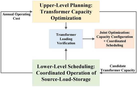
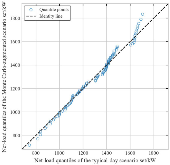
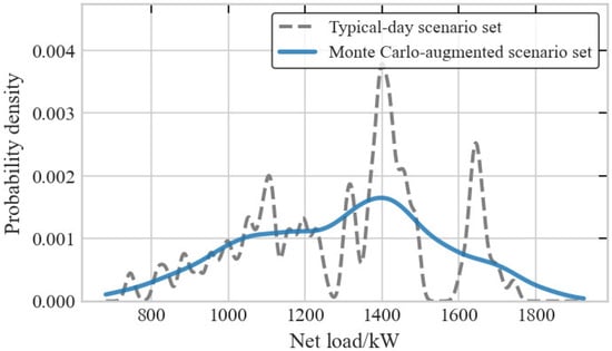
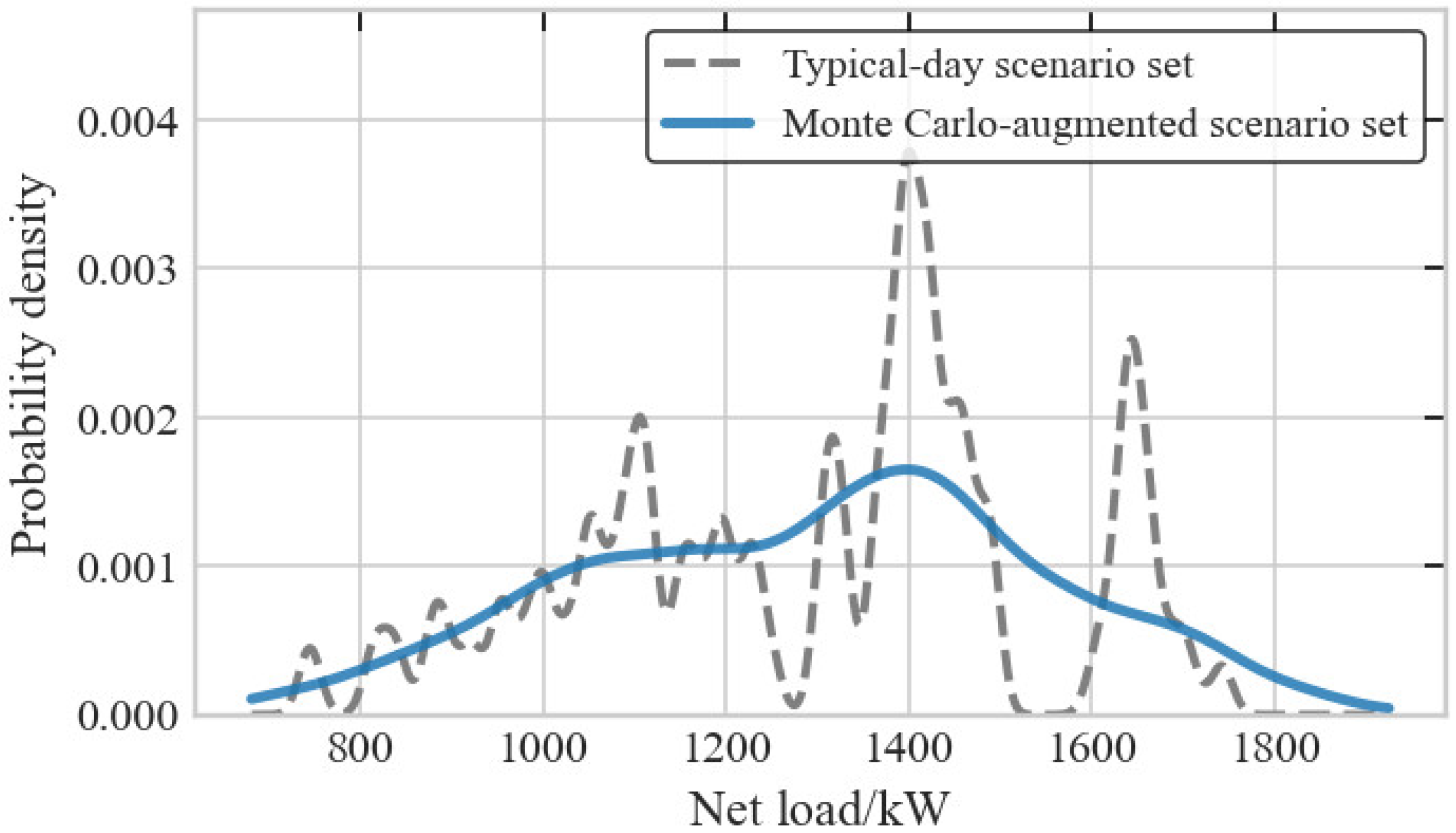
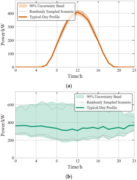
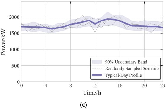
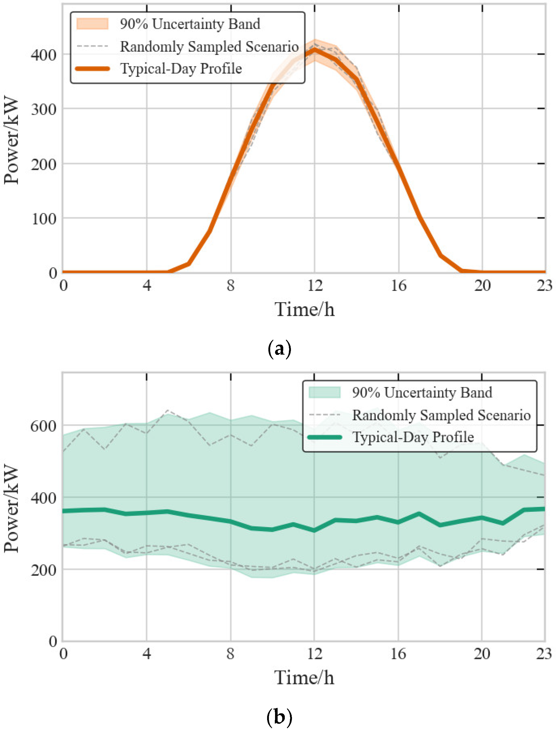
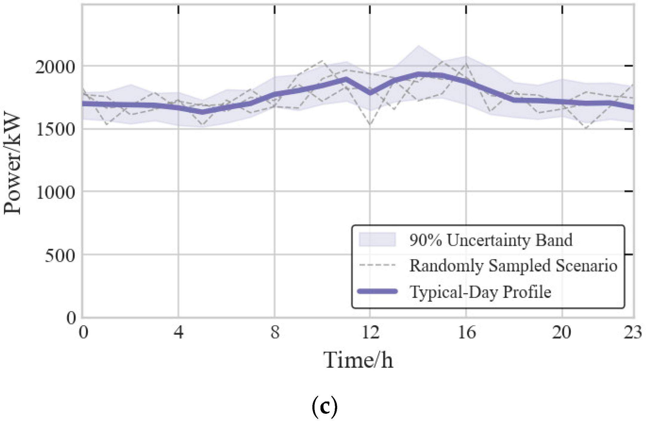
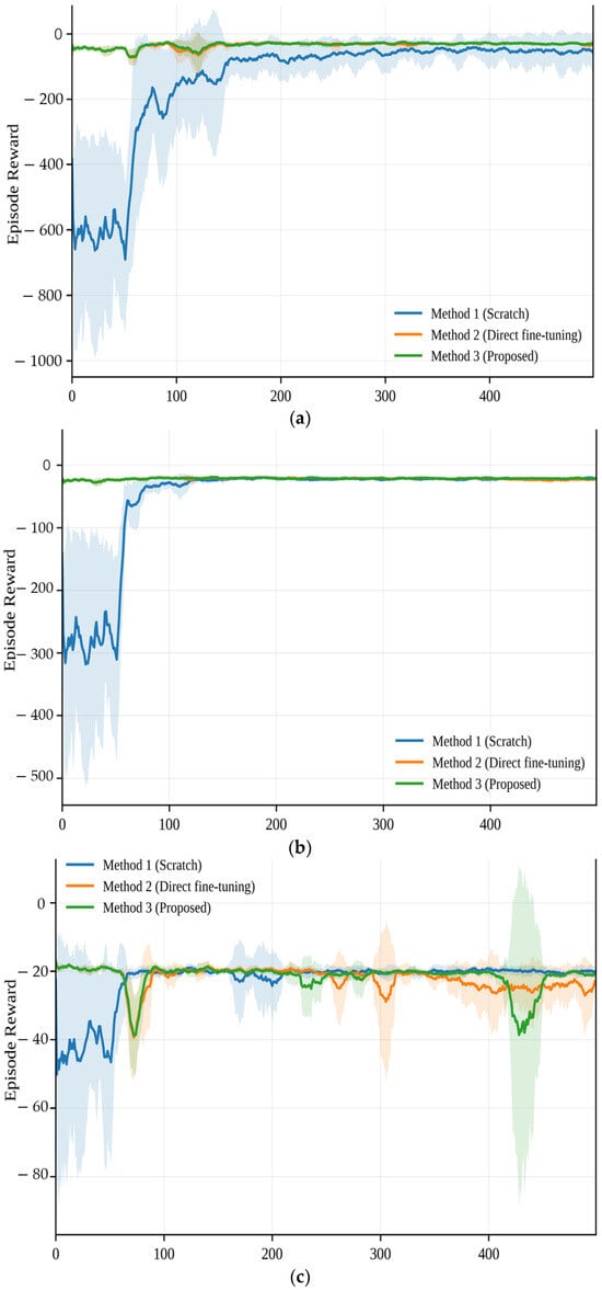
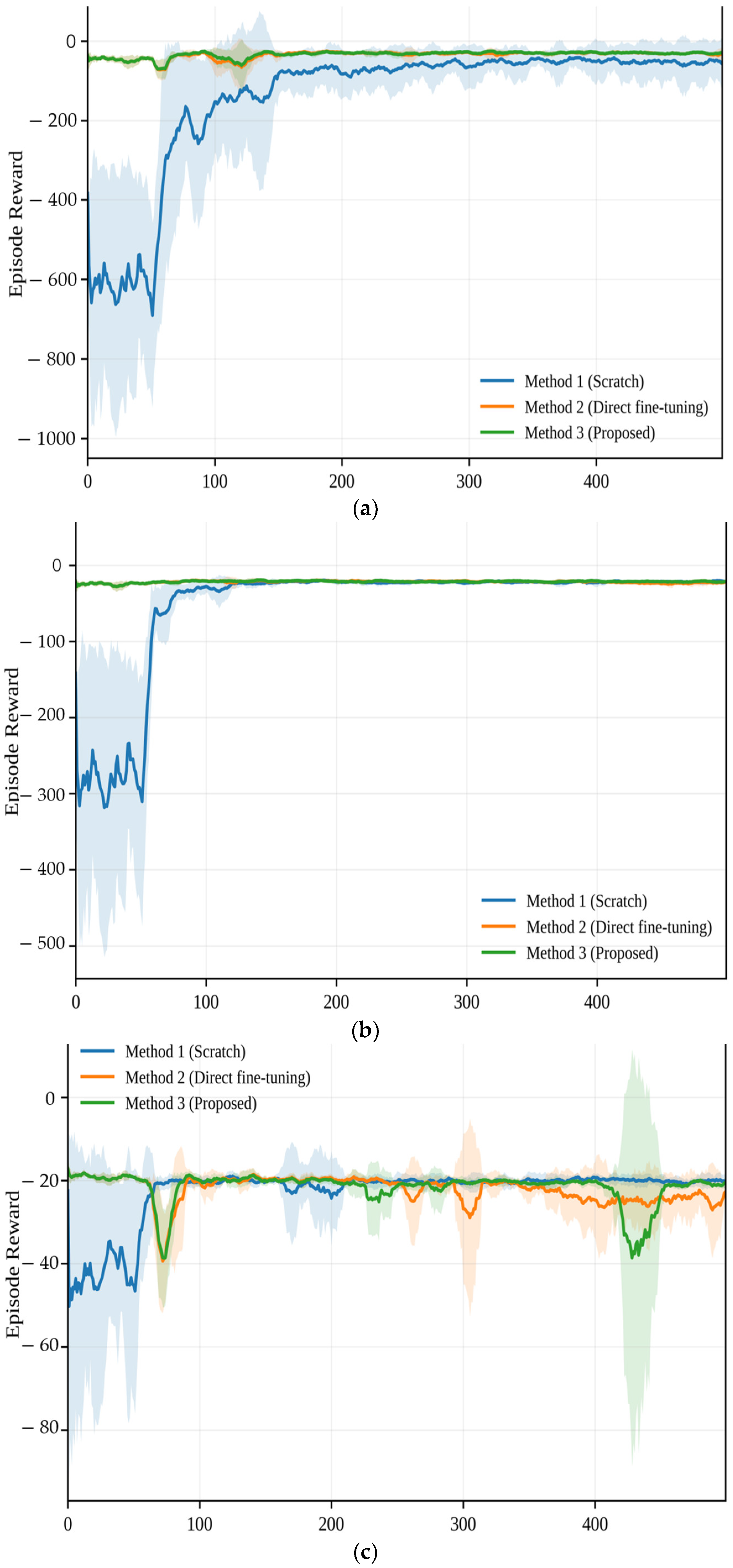
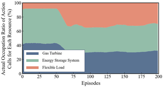
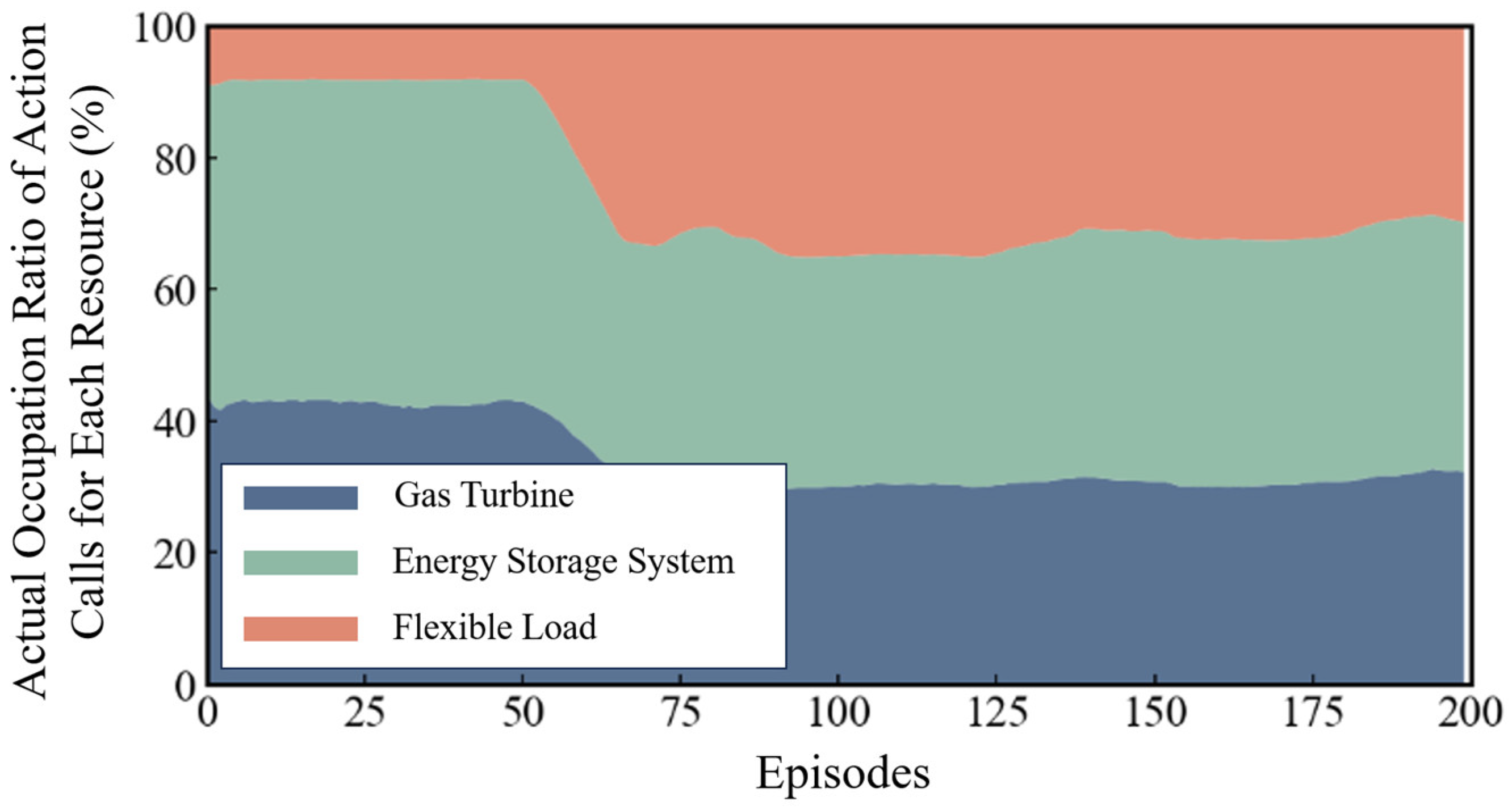
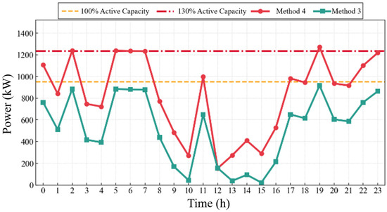
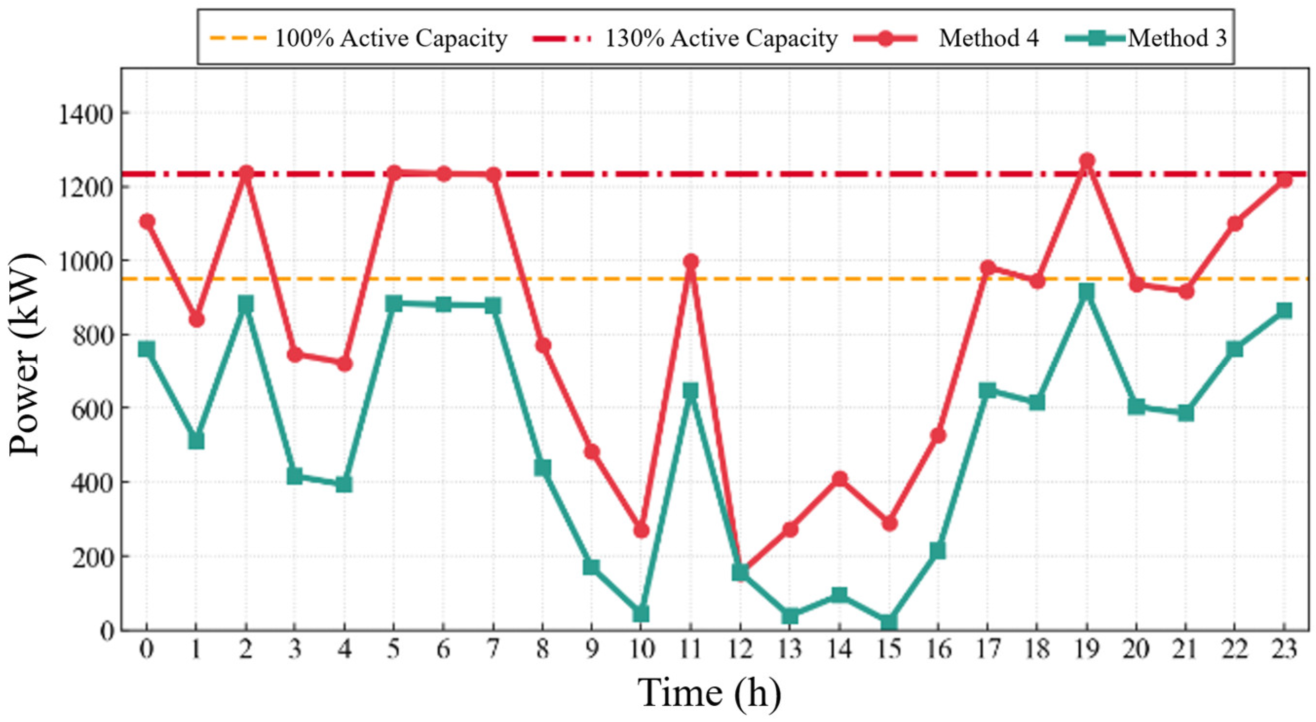
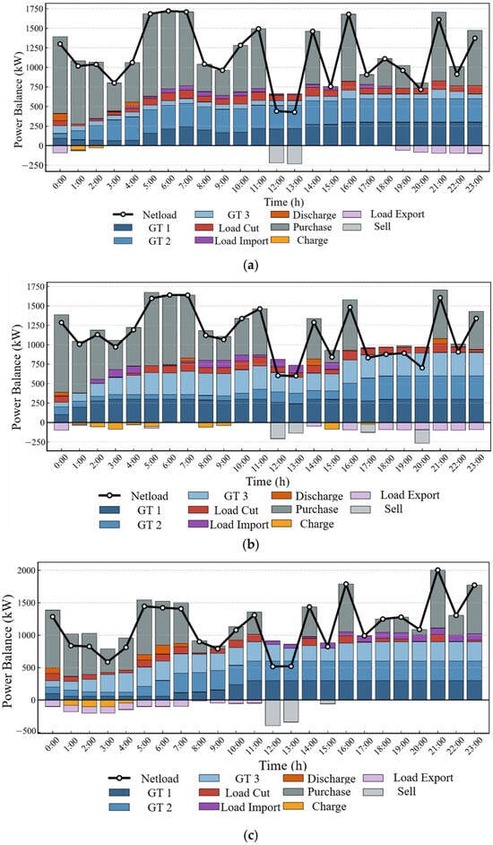
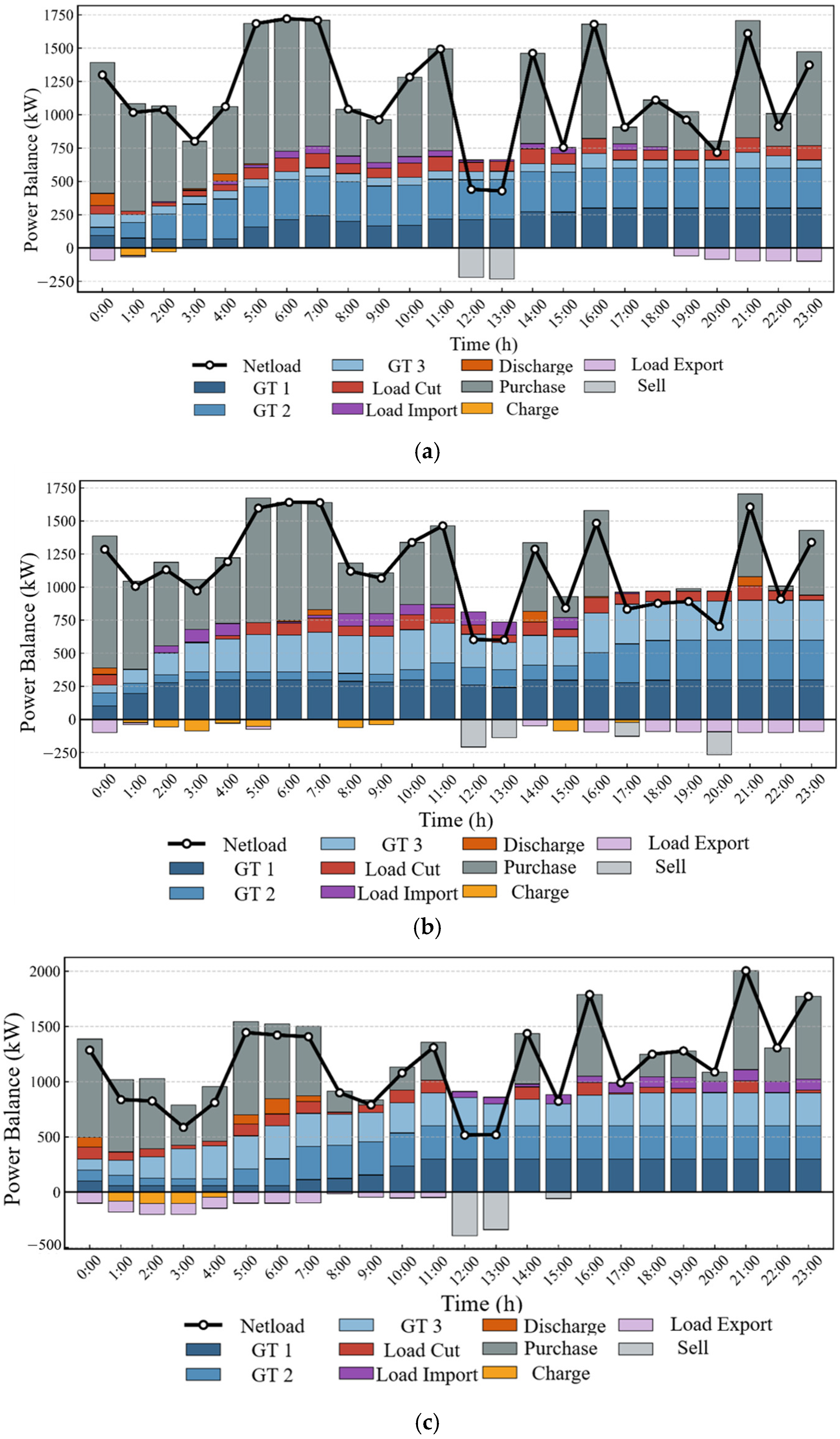

Disclaimer/Publisher’s Note: The statements, opinions and data contained in all publications are solely those of the individual author(s) and contributor(s) and not of MDPI and/or the editor(s). MDPI and/or the editor(s) disclaim responsibility for any injury to people or property resulting from any ideas, methods, instructions or products referred to in the content. |
© 2026 by the authors. Licensee MDPI, Basel, Switzerland. This article is an open access article distributed under the terms and conditions of the Creative Commons Attribution (CC BY) license.