


Abstract
We introduce Neural Operator Algebra in Hilbert Space (NOAH), a new framework that learns an adaptive family of operators instead of a single fixed mapping. Its spectral realization, F-NOAH, adds three physics-constrained generators, for advection, diffusion, and reaction, to a Fourier Neural Operator (FNO) backbone, and it restores their defining constraints exactly by closed-form projection after every optimizer step. We test the module in the regime that matters most in practice, a small training set and a short training budget: 500 initial conditions and 50 epochs on the two-dimensional Navier–Stokes equations at viscosity , trained at and evaluated zero-shot up to . The baseline is the Fourier Neural Operator as published. Over fourteen independent repetitions, F-NOAH attains the lower mean squared error in all 280 paired measurements, the pooled improvement is a factor of , and every cell remains significant after Holm correction. In the best run, the error falls by at and by at at . The NOAH module supplies a remarkable correction when data and computational resources are limited.
1. Introduction
This section sets out the scientific context, explains why the spectral domain is the natural place in which to represent the generators of a physical evolution, states the purpose of the study and the questions it is designed to answer, summarizes the methodological approach and the design tools, and lists the main findings. It closes by relating each research question to the part of the paper that resolves it.
1.1. Overall Context of the Problem
Approximating the solution operator of a parametric partial differential equation has become one of the central problems of scientific machine learning [1,2,3]. Neural operators learn a mapping between infinite-dimensional function spaces so that a single trained model can be evaluated for many initial conditions without the mesh dependence of classical finite-element [4] or finite-difference discretizations. The Fourier Neural Operator (FNO) of Li et al. [1] realizes this idea through spectral convolutions, and it inherits from the Fourier representation [5,6] a resolution invariance that makes zero-shot super-resolution possible in principle. The theoretical foundation for operator approximation by neural networks goes back to [7] and has since been developed for parametric problems in [8,9,10].
Two limitations of this paradigm motivate the present work, and both are structural rather than a matter of tuning.
- Learning is confined to a single regime.
A trained neural operator is one fixed operator. Applied to the Navier–Stokes equations, the kinematic viscosity selects qualitatively different dynamics: at , the flow is diffusion-dominated and relaxes to a few large vortices, whereas, at , it is advection-dominated and develops fine filamentary structure [11,12]. One fixed operator cannot represent both without conceding accuracy in at least one of them, because the balance between transport and dissipation is not a property of the input but of the regime. Conditioning a solver on the regime by meta-learning the discretization [13] addresses the symptom; we address the cause, by making the regime dependence explicit in the operator itself.
- No architectural encoding of operator structure.
Spectral convolutions are unconstrained. The vorticity form of the Navier–Stokes equations,
decomposes into an advection operator that conserves , a diffusion operator that dissipates enstrophy, and nonlinear residual interactions. A conventional architecture must rediscover this decomposition by gradient descent from data, which is sample-inefficient and produces a model whose internal state admits no physical reading. The cost of that rediscovery is the highest exactly when data are scarce, which is the setting this paper studies.
1.2. Why the Spectral Domain Is the Right Home for the Generators
The framework developed below could in principle be formulated in any representation of operators. That it is formulated spectrally is not a convenience inherited from the FNO backbone: the Fourier basis is the representation in which the generators of (1) become exactly the objects the framework requires them to be. Four properties make this so, and together they are the reason the construction of Section 3 and Section 4 works at all.
- The true generators are diagonal, and their symbols are known.
On the torus, the differential operators appearing in (1) are Fourier multipliers with symbols available in closed form:
The transport symbol is purely imaginary; the dissipation symbol is real and strictly negative away from the mean mode. These are precisely the skew-Hermitian and negative-definite conditions that define the constraint classes of Definition 2. The constraints imposed on the learned generators are therefore not an analogy borrowed from physics: they are the exact algebraic signature that the true generators of the governing equation possess in this basis, and a learned generator satisfying them belongs to the same operator class as the object it represents. In a nodal or finite-difference basis, the same operators are dense and non-normal, their spectral character is not visible entrywise, and no closed-form projection onto the corresponding classes is available.
- Constraints become checkable and enforceable wavenumber by wavenumber.
Because (2) is diagonal, membership in , or is a condition on one small matrix at each , and the projection onto each set is a two-line formula. This is what allows the constraints to be restored exactly after every gradient step rather than merely penalized, and it is the single feature that most sharply separates the present framework from physics-informed approaches acting through the loss alone [14,15,16].
- Composition becomes multiplication, so the algebra is tractable.
Operator composition in the spectral domain is the pointwise product of symbols, so the commutator required by the closure and Jacobi penalties of Section 4.4 costs two small matrix products rather than a composition of operators on a function space. The learned coefficients then form a third-order tensor [17] obtainable in closed form (Section 4.5).
- The learned physics is decoupled from the grid.
A symbol is indexed by wavenumber, not by grid point, so a generator trained at one resolution is evaluated unchanged at any other, with no interpolation and no retraining, and the classical accuracy theory of spectral methods [6,18] governs the truncation error. Resolution invariance is thereby a property of the representation rather than an empirical regularity of the fitted weights, a distinction that Section 5 makes precise and Section 7 tests.
1.3. Purpose, Scientific Questions, and Objectives
The purpose of this study is to determine whether replacing the learning of a single operator by the learning of a family of operators, generated by a small number of physically constrained elements, yields a neural operator that is more accurate under a fair and tightly matched comparison, and whether the gain is largest where it is most useful, namely, when the training set and the training budget are small.
Two scientific questions frame the work.
- SQ1. Can the algebraic structure that physics imposes on the constituent operators of an evolution equation, namely, skew-adjointness of transport, negative definiteness of dissipation, and self-adjointness of reaction, be imposed on a neural architecture as a hard constraint rather than as a penalty, and does doing so change what the model learns?
- SQ2. Does a constrained operator family help most in the small-data, short-training regime, where an unconstrained spectral operator has too few examples to locate the solution operator on its own?
These are made operational through four research questions.
- RQ1. Does learning a state- and time-dependent family instead of a fixed improve predictive accuracy on a standard Navier–Stokes benchmark, under a comparison in which the two models share every component except the algebra module?
- RQ2. Do the learned generators actually satisfy the algebraic properties the framework prescribes, and can this be checked rather than assumed from the presence of a penalty term?
- RQ3. Does a model trained at transfer to finer grids without retraining, and how does the size of its advantage behave as the grid is refined?
- RQ4. Is the advantage reproducible, in the strict sense that an independent repetition of the whole experiment reaches the same conclusion?
The objective is accordingly to construct the operator family, to describe what the construction does and does not provide, and to evaluate it against a matched baseline over five spatial resolutions and four rollout times, with the entire experiment repeated fourteen times.
1.4. The Setting: Few Samples, Few Epochs
The experiments in this paper use 500 training initial conditions and 50 epochs. That is a deliberately small budget, and it is the setting in which the question of an inductive bias is sharpest. Generating trajectories for a partial differential equation is expensive, and so is training on them: graphics processing units and the memory they carry are costly and often shared, and many groups that would like to use an operator surrogate cannot afford either a large dataset or a long schedule. A method that needs neither is worth more in practice than one that needs both. The results below show that the NOAH module supplies a good correction in exactly this regime, and that F-NOAH learns considerably better than FNO from few samples and few epochs.
Table 1 states the headline numbers. They come from the strongest of the fourteen independent runs, the one whose figures are shown throughout Section 7. That run is also the single outlier in the distribution of the fourteen, so the average is substantially smaller: over all fourteen runs, the improvement is a factor of , or about . Section 7.5 summarizes the full statistical analysis and Appendix B gives the details.
Table 1.
Reduction in mean squared error of F-NOAH relative to FNO at the final rollout time , in the best of the fourteen runs. Both models were trained at on 500 initial conditions for 50 epochs, and they were evaluated zero-shot at the four finer grids.
1.5. Methodological Approach and Design Tools
The methodological approach has three components. First, an analytical component formulates the operator family in the Banach algebra of Fourier multiplier operators [5,19] and fixes three constraint manifolds corresponding to the three physical processes. Second, an architectural component realizes the family as a differentiable module: generators are stored as complex spectral symbols, projected onto their manifolds in closed form after every gradient step, and combined by control weights predicted from global field statistics and the target time. Third, an experimental component compares the resulting model with the original FNO under an identical training protocol, on data generated by a pseudo-spectral solver, with the whole experiment repeated fourteen times and assessed by paired tests (Section 7.5).
The claim we make is deliberately bounded, and we state it here so that the rest of the paper is read against it. F-NOAH attains lower error than a closely matched FNO on the cases evaluated here, and the margin is large in a regime of few samples and few epochs. Those cases involve two-dimensional freely decaying Navier–Stokes flow at a single viscosity, five resolutions, and four rollout times; they illustrate what the construction can do rather than survey where it holds. The far larger benchmark program that the Navier–Stokes system admits, across forced and unforced regimes, viscosities, training set sizes, and training budgets, is set out in Section 9 rather than attempted here, and we regard it as work for the community.
The design tools are as follows. Reference trajectories are produced by a semi-implicit Crank–Nicolson pseudo-spectral solver with two-thirds-rule dealiasing [20], implemented entirely through the Fast Fourier Transform (FFT) [21]. Initial conditions are drawn from a Gaussian Random Field (GRF) with a Matérn-type covariance [22]. Models are implemented in PyTorch (version 2.11.0+cu128) and trained with AdamW [23] under a ReduceLROnPlateau schedule; all figures are generated by the authors’ own evaluation scripts using Matplotlib (version 3.10.0).
1.6. Main Findings and Contributions
The study yields the following findings, each established in the section indicated.
- 1.
- 2.
- A comparison with matched normalization (Section 7.1). The baseline is the Fourier Neural Operator as published, which uses no normalization in its spectral blocks; neither does the F-NOAH backbone. The two models share the lifting, the coordinate grid, the absence of padding, the truncation, the width, the depth, the projection head, the input residual, the optimizer, the schedule, the clipping, the epoch budget, the data, and the test sets, and their parameter counts differ by , or , which is exactly the size of the module. One difference outside the module remains and we state it rather than suppress it: the F-NOAH trunk uses a residual spectral block while the baseline uses the published non-residual one. Section 7.1 sets out what the comparison can and cannot therefore attribute.
- 3.
- Accuracy in the small-data regime (Section 7.2). With 500 training initial conditions and 50 epochs, F-NOAH reduces the mean squared error at by at the training resolution, by at in the best run, and by to over the whole grid of five resolutions and four rollout times. Over all fourteen runs, the pooled improvement is a factor of .
- 4.
- Reproducibility over fourteen runs (Section 7.5, Appendix B). The entire experiment was repeated fourteen times. F-NOAH attains the lower error in all 280 paired measurements, with no reversal. Every one of the twenty (resolution, rollout time) cells reaches the exact Wilcoxon floor for and remains significant after Holm correction. The pooled improvement is a factor of with confidence interval , each run’s own improvement factor lies between and , removing any single run leaves all twenty cells favoring F-NOAH, and a prediction interval built from the fourteen runs assigns probability to a fifteenth run favoring F-NOAH.
- 5.
- Two structural effects (Section 7.5). The advantage grows with rollout time, from a factor of at to at , and narrows as the test grid is refined, from at to at at the final time. The second effect has a clear cause: the error of the original FNO is almost flat in resolution, while that of F-NOAH rises by over a sixteenfold refinement. F-NOAH is the more accurate model at every resolution tested, and it is the less resolution-stable of the two. We state this plainly rather than report only the aggregate.
- 6.
- Interpretability (Section 7.3). The prediction splits into an advection, a diffusion, and a reaction component, each with a constrained spectral symbol, and the control weights are the same at all five test resolutions. No comparable decomposition is available from the baseline. The assignment is measured at one viscosity, so it shows that the decomposition is stable under grid refinement, not that it tracks the physical regime.
1.7. Relation to Prior Work
The framework sits at the intersection of five lines of research, and its contribution is best understood by what it changes in each.
- Neural operators.
The FNO [1,3], the graph kernel operator [24], and DeepONet [2,25] established operator learning and resolution-independent generalization, with approximation-theoretic underpinnings in [7,8,9,10]. Extensions address non-uniform geometries [26], graph discretizations [27,28,29], multiscale bases [30,31], convolutional encoder–decoder backbones [32], and attention mechanisms [33,34]. All of these learn a single operator. NOAH replaces it by a family built from a small set of constrained generators, which is what permits state- and time-dependent behavior within one trained model.
- Physics-informed learning.
Physics-Informed Neural Networks (PINNs) [14,35,36] enforce physics through residual penalties, leaving the architecture unconstrained; the same philosophy has been applied to flow reconstruction [37], to surrogate modeling [15,38], to operator regression [16], and to solver-coupled training [39]. Hamiltonian [40], Lagrangian [41], and symplectic [42] networks preserve structure for conservative systems. We extend the structural philosophy to dissipative problems through Banach algebra representations [19,43], with constraint manifolds maintained by projection after each gradient step in the spirit of structure-preserving integration [44].
- Geometric deep learning.
Group-equivariant networks [45,46,47], and their relaxations to approximate symmetry [48], constrain the network map to commute with a symmetry action. Our constraint is placed elsewhere: on the learned operators themselves. The resulting bias encodes which processes are active and at what relative strength, rather than which transformations leave the equation invariant, and the two are complementary.
- Control theory, dynamical systems, and operator algebras.
The correspondence between Lie algebras and reachability is classical [49,50,51,52], as are semigroup generation results for advection and diffusion operators [53,54] and the closure properties of -algebras [43,55]. A parallel line views network depth itself as a dynamical system [56,57,58,59,60], and a further one recovers governing operators from data by sparse regression [61] or by linear embedding [62]. What is new here is the use of the operator algebra as a design principle for a neural operator with learned, state-dependent control weights.
- Data-driven closure and geophysical applications.
Neural closures for subgrid-scale turbulence [63,64,65] typically presuppose a turbulence model or require large datasets; the control weights act as a learned dynamic closure without either, which is one reason the construction is attractive when data are scarce. Large-scale operator models for weather [66,67,68] operate at fixed resolution, whereas resolution transfer and regime adaptivity are precisely the properties needed for downscaling and ensemble prediction. Regime adaptivity is a design property of the state-dependent weights that this study does not test, since all experiments are at a single viscosity (Section 9).
1.8. Organization of the Paper
Section 2 fixes the notation and recalls the functional-analytic material the construction consumes: Fourier multiplier operators, the three symbol classes, and the Lie bracket. Section 3 defines the NOAH framework, replacing the fixed operator by a family, identifying the physical content of the three generator classes, and stating what the construction provides and what it does not; this answers RQ1 at the level of formulation. Section 4 develops the spectral realization F-NOAH, from its architecture and generators through the control weights, the physics regularization, the bracket coefficients, and the algorithms, to the comparison with the FNO baseline; it makes RQ1 testable and sets up the check required by RQ2. Section 5 treats geometric consistency on the torus and states what the correction operator guarantees at any resolution; it supplies the structural basis for RQ3. Section 6 formulates the two-dimensional Navier–Stokes learning problem, the solver, the datasets, and the provenance of every figure. Section 7 reports the experiments, beginning with the training protocol and what the comparison controls for, then one representative run in detail, the operator decomposition, the statistical analysis over all fourteen runs, and the discussion. It answers RQ1 through the matched accuracy comparison, RQ2 through the verification subsection, RQ3 through the super-resolution results, and RQ4 through the fourteen repetitions. Section 8 answers the four research questions in turn and restates the statistical evidence in compact form. Section 9 states the limitations of the study and the benchmarks that would settle the questions we leave open. A list of abbreviations and of principal symbols follows; Appendix A collects the functional-analytic background, and Appendix B the full statistical analysis of the fourteen runs.
2. Mathematical Preliminaries
This section fixes the notation used throughout and recalls only those notions that the construction of Section 3 actually consumes: Fourier multiplier operators and the algebra they form, the three spectral symbol classes that encode transport, dissipation, and reaction, and the Lie bracket. The standard background on Banach and Hilbert spaces, spectral theory, and -algebras is collected in Appendix A so that it does not interrupt the development.
2.1. Fourier Multiplier Operators
The domain throughout is the flat torus with doubly periodic boundary conditions, and the state space is . For sampled on a uniform grid, denotes the Fourier coefficient at wavenumber and , the forward and inverse transforms. The Plancherel identity [5,69] is used without further comment.
Definition 1 (Fourier multiplier operator and its symbol).
An operator is a Fourier multiplier [5,70] if there is a map , the symbol, with
denotes the set of such operators, and , where is the spectral norm [71,72].
Two facts make the right ambient space for the construction, and both are immediate from Definition 1. Composition acts on symbols by pointwise matrix product,
so that is a unital Banach algebra with unit the identity, ; the adjoint of a multiplier is the multiplier with symbol , so the algebra is closed under involution. Consequently every operation performed on the generators during training, including the constraint projections of Section 4.2, keeps them inside .
2.2. Symbol Classes and the Lie Bracket
The physical content of the framework enters through three classes of symbols, distinguished by where their eigenvalues lie.
Definition 2 (Physics-constrained symbol classes).
For a fixed truncation and a fixed margin , define
collects the skew-Hermitian symbols and encodes advection, the negative-definite symbols and encodes diffusion, and the Hermitian symbols and encodes reaction. Note that , so the diffusion class is distinguished from the reaction class only by the sign condition on the spectrum. Let denote the corresponding operator classes, that is, the Fourier multipliers whose symbol lies in the respective set at every retained .
Definition 3 (Lie bracket and structure constants).
For the bracket is the commutator , whose symbol is . Given generators , the coefficients in
are the structure constants [73,74,75]; viewed as an array indexed by , they form a third-order tensor [17]. The span is a Lie algebra precisely when (8) holds with equality and the Jacobi identity is satisfied.
This definition is stated for matrix-valued symbols, , for which the pointwise commutator is generally non-zero. The realization of Section 4 uses scalar symbols, for which it vanishes identically. The paragraph on the array bracket in Section 4.2 states precisely which bracket the trained model penalizes and on which object the algebraic claims of this paper are therefore made.
We stress at the outset that in the trained model (8) is an approximation enforced by a penalty, not an identity. Which parts of the structure hold exactly and which only approximately is the subject of Section 7.4.
3. Neural Operator Algebra in Hilbert Space
This section defines the framework. It first states the mapping that replaces the fixed operator of conventional neural operator learning, then identifies the physical meaning of the three generator classes, and finally records what the construction guarantees. The results are deliberately stated in restricted form: each is proved under hypotheses that the architecture actually satisfies, and the scope of each is delimited immediately afterward.
3.1. From a Fixed Operator to an Operator Family
A neural operator learns a single map between function spaces. NOAH learns instead a family indexed by the physical regime and by the state,
where parameterizes the regime, for instance, the viscosity, and is a family of generators satisfying the constraints of Definition 2. The family is realized by a state-dependent linear combination of the generators applied as a correction to a latent field :
with a residual scaling factor [76] and the projection back to the output space. The control weights are produced by a network from global statistics of and the target time, and they are recomputed at every forward pass; their construction is given in Section 4.3.
Figure 1 contrasts the two settings geometrically. A neural operator occupies a single point of operator space; NOAH occupies the submanifold swept out as ranges over its domain.
Figure 1.
Operator space: a single point for neural operators, a manifold for NOAH.
Figure 2 places the two alongside a conventional neural network, making explicit the input and output spaces and the capability each level adds.
Figure 2.
Input and output spaces of a neural network, a neural operator, and NOAH.
3.2. Physical Meaning of the Three Generator Classes
The choice is dictated by the structure of (1), whose three terms are transport, dissipation, and residual nonlinear interaction. The three constraint sets of Definition 2 are chosen because they are the algebraic signatures those three processes carry in the Fourier basis: skew-adjointness for transport, negative definiteness for dissipation, and self-adjointness for reaction [53,54,77,78].
The energetic statements that motivate this choice are standard. Let Ł be a bounded operator on . If then , so the norm is conserved. If and for all u, then for . If then the spectrum of Ł is real ([79], Thm. VI.8).
We must be exact about which of these the realization of Section 4 actually delivers, because the generators act as Fourier multipliers with scalar symbols and the relevant condition is therefore a condition on each symbol value , not on the array as a matrix. Writing , the multiplier has , so norm conservation requires at every retained , contraction requires at every retained , and a real spectrum requires at every retained .
Measured against that criterion, the three generators are not on the same footing, and we set out the position plainly.
- , diffusion. The projection is applied entrywise, so holds at every retained wavenumber after every optimizer step. The contraction property for therefore holds exactly for the trained model. The diffusion generator can remove energy and cannot add it. This is the one energetic statement in the paper that is a theorem about the model as implemented.
- , advection. The projection makes the array skew-Hermitian as a matrix. That forces on the diagonal, but off the diagonal it imposes only the pairing , which leaves free. Norm conservation therefore holds on the diagonal of the retained band and is not established elsewhere. We do not claim that is energy preserving.
- , reaction. By the same argument, Hermiticity of the array makes real on the diagonal and leaves the off-diagonal symbol values complex. We do not claim that has real spectrum as a multiplier.
The constraints on and are nonetheless exactly enforced and are not vacuous: they fix the arrays inside the skew-Hermitian and Hermitian subspaces of , which is the space in which the closure and Jacobi penalties of Section 4.4 operate, and (11) shows that those two subspaces together span the whole of over . What does not follow is the operator energetics, and the reason is a mismatch between the level at which the constraint is imposed, the array, and the level at which the generator acts, the individual symbol value. Aligning the two would require replacing the matrix projections by the entrywise conditions and , which are equally cheap and equally closed-form. We did not do this in the runs reported here, we list it in Section 9 as the first change we would make, and in the meantime we label the three components of Section 7.3 by the process each is intended to represent rather than by an energetic property we have established.
One further point of precision concerns the margin. Definition 2 asks for a uniform in the diffusion class, whereas the projection enforces the closed condition , that is, . What holds exactly is the weaker statement, that generates a contraction semigroup. Strict exponential decay at a uniform rate is not guaranteed and we do not claim it. The weaker statement is also the one the physics requires: a dissipative generator must not create energy, but it need not damp every mode at a rate bounded away from zero, and indeed the true viscous symbol vanishes at .
3.3. What the Construction Provides
Three questions arise naturally: whether three constrained generators are expressive enough, what the bracket structure buys, and in what sense the model is controllable. We answer each in the restricted form the construction supports, and state the limits of each answer.
- Expressivity.
Regard as a vector space over . The skew-Hermitian set and the Hermitian set are then -linear subspaces, each of real dimension , and every matrix splits uniquely as , so
The symbol of an arbitrary truncated Fourier multiplier therefore decomposes uniquely into a skew-Hermitian and a Hermitian part, so nothing representable by an unconstrained truncated multiplier is excluded in principle by the choice of classes.
This is a statement about the linear span of the constraint sets, not about the trained model, and it is deliberately weaker than a universal approximation theorem of the kind available for feedforward networks [80,81,82] or for operator networks [7]. It does not say that the learned , being three fixed elements rather than a basis of , approximate an arbitrary target operator; the adaptive weights supply only a three-parameter family at each forward pass. The negative-definiteness condition (6) additionally restricts to a convex subset of , which is a genuine and physically intended loss of generality.
- Closure and the role of the bracket.
The bracket enters the architecture through the penalties of Section 4.4, which push toward the span of the generators. Closure is what makes repeated composition of the learned corrections stay within the modeled family, and is therefore the property that would justify calling a Lie algebra. It is not enforced exactly. Section 7.4 states what is checked and what is not.
- Reachability.
Fix a wavenumber and consider on the bilinear control system
Let be the real Lie subalgebra of generated by , and let be the connected Lie subgroup with that Lie algebra. Since each is real, lies in for almost every t, and a control system whose system matrix takes values in a Lie subalgebra evolves inside the corresponding subgroup ([49,50], Ch. 2). The set of states reachable from is therefore contained in .
This is an inclusion, and it bounds what the architecture can produce. The converse, that the whole of is reachable, would require a Lie algebra rank condition [52,83], which we neither verify nor impose: with fixed generators the algebra they generate is in general a proper subalgebra of , so full controllability on should not be expected. The hyperbolic tangent of Section 4.3 supplies controls of both signs so that particular obstruction is absent, but the rank condition remains unchecked. We therefore say only that the family generated by the model is governed by , and we do not claim controllability in the sense of reaching an arbitrary target.
- Relation to the exponential map.
The correction (10) is the first-order truncation of the group action, , which is accurate because the generators are initialized at scale and the residual factor keeps the correction small relative to the latent field. Higher-order terms could be retained at the cost of one additional spectral product each; we do not perform that here.
4. F-NOAH: The Spectral Realization
This section turns the framework of Section 3 into a differentiable architecture. It states the composite map, constructs the three generators and the projections that keep them on their manifolds, derives the adaptive control weights, defines the physics regularization, and gives the algorithms in compact form. The section closes with the parameter and complexity accounting that makes the comparison with the Fourier Neural Operator in Section 7 a matched one.
4.1. Architecture
F-NOAH composes a spectral feature extractor with the operator algebra correction. Writing for the lifting into a latent space of width d, for L standard Fourier layers, and for the projection back to the output space,
where is the latent field, is the identity that makes the algebra block residual, and with pointwise convolutions and the Gaussian error linear unit. In the Fourier domain the correction is a pointwise product,
so the whole block costs one forward and one inverse transform, , plus scalar multiplications.
Three consequences follow immediately from (14). The cost is that of the fast Fourier transform [6,21]. The symbols are indexed by wavenumber rather than by grid point, so a trained model is evaluated at any resolution without retraining or interpolation [3]. And, because Fourier multipliers map into itself, the correction cannot introduce spatial asymmetry, a point developed in Section 5.
Figure 3 shows the composite architecture together with the internal structure of one Fourier layer, and Figure 4 expands the algebra module itself.
Figure 3.
Architecture of F-NOAH, of one Fourier layer, and of NOAH.
Figure 4.
Internal structure of the NOAH module.
The top panel of Figure 3 traces the path of an input vorticity field through grid augmentation, lifting, the L Fourier layers, the algebra module, and the projection with its residual skip. The data are periodic, so no zero padding is applied in either model. The middle panel resolves a single Fourier layer into its spectral convolution, its pointwise convolution, and their nonlinear combination. The bottom panel isolates the NOAH block, which is the only component not present in a standard spectral neural operator.
Figure 4 shows the two streams that meet inside the module: the latent field is transformed to the frequency domain and multiplied by each generator symbol, while the field statistics and the target time are combined by the control network into the weights that scale the three resulting components before they are summed and transformed back.
4.2. The Generators and Their Projections
Each generator consists of two complex symbol arrays , with , one for each sign band of as in (20). Each array is obtained by projecting an independently drawn random matrix onto the constraint set of its generator, and is thereafter updated by gradient descent under repeated projection.
Table 2 collects the construction, the constraint it enforces, the resulting spectrum, and the physical reading, for the three generators. To keep the notation light the table is written in terms of a single symbol array ; every row applies verbatim and independently to both and , so the two arrays of a generator always satisfy the same constraint, and a statement such as “ is skew-Hermitian” should be read as holding for each of its two arrays. Initialization draws
the small scale ensuring that the correction begins as a mild perturbation of the latent field. A fresh A is drawn for each of the arrays and is discarded after projection. For , the initialization additionally scales the imaginary part by so that the diffusion generator starts close to a real, purely damping multiplier; the constraint projection applied thereafter leaves the imaginary part free.
Table 2.
Construction of the three generators, where the constraint acts, and what it does and does not establish. Each row holds for both symbol arrays of a generator.
The three projections are closed-form and idempotent: gives skew-Hermiticity of the array, gives Hermiticity of the array, and replacing by makes every entry of have a non-positive real part.
One distinction must be drawn before Table 2 is read. The array enters the model in two ways. In the forward pass (19) it acts entry by entry: the Fourier coefficient at wavenumber is multiplied by the single complex number , so the operator is a Fourier multiplier whose spectrum is the set of entries . In the penalties of Section 4.4 the same array is used as a matrix, through the commutator (18). The matrix projections, for and , therefore constrain the array in the sense the penalties use and not in the sense the forward pass uses, whereas the projection for is entrywise and does constrain every symbol value. Table 2 records this row by row, and Section 3.2 states which energetic readings follow and which do not.
Gradient descent moves off its constraint set in general. After every optimizer step the projection is therefore reapplied in place,
where is the projection onto the i-th constraint set of Table 2, applied to and alike. This hard projection is what distinguishes the framework from a penalty-only approach: the constraints in Table 2 hold exactly at every point of training at which the model is evaluated, to machine precision, whereas the closure and Jacobi properties of Section 4.4 are only encouraged.
Definition 4 (Isotropy).
A frequency-domain operator is isotropic if it applies the same complex scalar to every channel of its input at frequency ,
- Which bracket the model penalizes.
Definition 4 has a consequence for Definition 3 that must be stated before the penalties of Section 4.4 are introduced. Under isotropy the symbol at each retained wavenumber is a scalar, , and the operator product of two generators has symbol by (4). Scalars commute, so
and the operator algebra generated by isotropic Fourier multipliers is abelian. Definition 3, read as a statement about operators on , is therefore vacuous in the isotropic case: it is non-trivial only for the channel-mixing symbols for which it was stated.
The bracket that the penalties of Section 4.4 actually act on is a different one. Each generator stores its symbol as a array indexed by the two wavenumber components, and the penalties evaluate the matrix commutator of those arrays,
with the Frobenius norm on . This is a matrix product over the mode grid, not a composition of operators: it does not correspond to applying and then to a field, and (17) is untouched by it. Equation (18) is the bracket meant wherever appears from Section 4.4 onwards.
We therefore make no claim that the trained generators form a non-abelian Lie algebra of operators; by (17) they cannot. What the penalties do is impose closure, Jacobi, and a norm target on the symbol arrays within , a structural regularizer on the symbol parameterization, and the object whose structure Section 7.4 discusses is that array algebra. The empirical question it raises, whether constraining the arrays in this way changes what the model learns, is answered affirmatively by the experiments, independently of the interpretation of the constraint. Recovering a non-trivial operator bracket would require restoring channel-mixing symbols, at a cost of a factor in frequency-domain parameters; that trade-off is taken up in Section 9.
Isotropy separates two concerns that a standard spectral layer conflates. The physics operator acts identically on all latent channels, while channel mixing is left to the pointwise convolutions in the lifting, the local bypass, and the projection. Three benefits follow: the number of frequency-domain parameters drops from for a spectral layer to per generator, counting both symbol arrays of (20), a factor of at the configuration used here; the commutators in Section 4.4 become tractable computations; and each generator admits a single physical reading rather than one per channel. Writing for a learnable scalar gain, the forward pass of the module is
where the real transform indexes over both signs while is non-negative. Each generator therefore stores two arrays of scalars, for the lowest positive band of and for the corresponding negative band, and the symbol is assembled as
with for . The shift by K in the second line maps onto the rows of . This mirrors the two weight tensors of a standard spectral convolution, which treats the two bands independently for the same reason. Both arrays are held on the same constraint manifold and both are restored by the projection (16), so (20) defines a single Fourier multiplier and the periodicity argument of Section 5 applies unchanged. Since symbols vanish outside the two bands, the correction acts only on the lowest K modes in each direction.
The three components that (19) produces at are shown and discussed in Section 7.3, together with the control weights that scale them.
4.3. Adaptive Control Weights
The weights decide how strongly each generator contributes at a given forward pass. They are functions of the latent field and of the target time t, and they are recomputed at every call, which is what makes the operator family state- and time-adaptive rather than fixed. The map is built in five stages, summarized in Table 3.
Table 3.
The five stages mapping latent field and target time to the control weights.
The scalar t is first lifted to by logarithmically spaced sinusoids,
a fixed map with no learnable parameters, of the form introduced for positional encoding in sequence models [34], which makes nearby times produce similar vectors and distant times nearly orthogonal ones. A two-layer network with Gaussian error linear units then reshapes it into a learned embedding , computed once per forward pass.
In parallel, the latent field is reduced to a global descriptor. The choice of descriptor matters more than it may appear, and it is dictated by the requirement that the control weights be the same at every test resolution. Order statistics such as the spatial minimum and maximum do not have that property: they are extremal values over the grid, so they drift as the grid is refined and more of the field is resolved. The descriptor is therefore built from integral functionals of band-limited projections only. Writing for the projection onto , and setting
the four per-channel numbers are
where is the spatial mean and the root mean square deviation from that mean, both taken without Bessel correction. The first number is the large-scale offset, the second the total energy in the band the generators act on, and the third and fourth split that energy between the lower and the upper half of the band.
Two properties of (23) matter later. It is invariant under spatial translation and under the periodic identification , since every entry is an integral functional over the whole torus; this is used in Section 5. And it is exactly independent of the grid: for a field band-limited to K modes, both the field and its square have bandwidth at most , so the discrete grid averages are exact quadratures whenever , which at holds already at . The four numbers are therefore identical at 64, 128, 256, 512, and 1024, which is why the control weights reported in Section 7.3 do not move with resolution.
The two streams are concatenated, with no intermediate projection:
which for and gives an input of width 256. The relative weight of the two streams is therefore fixed by their dimensions, for the field statistics against for time, a ratio of three to one in favor of the field. This is appropriate for F-NOAH, where is the output of L deep spectral layers and its statistics are informative; a backbone-free variant, in which the algebra module acts on a linearly lifted input, would carry little information in and would call for a larger time share. We note this as a design consideration rather than a result, since only the F-NOAH configuration is trained and evaluated here.
The concatenated vector is normalized once, by a layer normalization [84] over its entries, before it enters the control network. This is a guard against saturation: the four statistics of (23) and the time embedding are on unrelated scales, and without it the closing hyperbolic tangent saturates on the larger of the two streams. A three-layer network then maps the result to logits, with a second layer normalization after its first linear map and dropout at rate , the latter active in training only:
Both normalizations act on vectors of global scalars inside the control network. Neither touches a field, and neither has any counterpart in the baseline, which has no control network.
The output activation is the hyperbolic tangent,
and the choice of a signed activation is deliberate. A generator may need to be subtracted as well as added: the constraint sets and are symmetric under , so the direction in which a Hermitian or skew-Hermitian generator acts is not fixed by its constraint and must be supplied by the coefficient. Restricting to the positive half-line would remove that freedom and force the model to encode sign changes inside the generators, where they would compete with the constraint projection. The magnitude is then read as the strength with which process i participates, and as its direction.
Two consequences of (26) should be recorded, since both are visible in the trained models. First, tanh saturates, and at , the diffusion and reaction coefficients do saturate, reaching (Section 7.3); the model is operating at the boundary of its coefficient range, so the reported values should be read as “this process is switched fully on” rather than as a finely resolved weight. Second, because is closed under sign inversion, the pairs and give identical predictions, so the sign of an individual coefficient is a gauge choice fixed only by initialization; only the product is determined by the data. This is recorded as a property of the parameterization that must be kept in mind when coefficient signs from different runs are compared.
A further scalar gain , initialized to 1, multiplies each generator in (19). It is a free amplitude that the optimizer may use to rescale a generator relative to the others; it does not enter the reported coefficients, which are the raw activations (26).
Table 3 presents the same five stages in compact form, with the output, the formula, and the role of each; it is the reference to consult when reading the control-weight algorithm of Section 4.6.
Table 4 lists the parameters the module introduces, at the configuration actually trained in Section 7: latent width , , , , and a single algebra module instantiated once after the L spectral layers, as Equation (13) and the training algorithm of Section 4.6 specify. Complex symbols are counted as one parameter per complex entry, which is the convention under which the totals are reported. The module adds parameters, and the baseline has no component that the module replaces, so the difference between the two totals is exactly the module: . The module is therefore about of the model.
Table 4.
Learnable parameters of the algebra module, with , , , .
4.4. Physics Regularization
Three penalties act on the generators. They do not constrain the prediction directly; they shape the algebra spanned by the symbol arrays. Throughout this subsection denotes the matrix commutator (18) of the arrays, not the operator commutator of Definition 3, for the reason set out in Section 4.2.
where are learnable, is the set of triples with distinct, and, importantly,
is the set of ordered pairs with . The restriction is not a simplification but a consequence of antisymmetry: makes the reversed pair redundant and makes the diagonal vacuous, so the coefficients indexed by determine the remaining 18 of the . How all 27 are obtained from those 9, and why no separate parameters are needed for them, is the subject of Section 4.5. Each of the three brackets is evaluated on both symbol arrays of (20), and the losses are averaged over the two. The first penalizes failure of closure, the second failure of the Jacobi identity, and the third drives the bracket norms toward a target , keeping the generators neither commuting, in which case the algebra would be trivial, nor so non-commutative that the first-order truncation of the group action becomes inaccurate. The total objective is
with the mean squared error. The small weight is deliberate: the algebraic structure is to be learned without displacing the data-fitting objective.
4.5. How the Bracket Coefficients Are Obtained
The coefficients of (27) are the only quantities in the model that are not either a network parameter trained by the data loss or a constrained symbol array. This subsection states plainly where they come from, because the answer bears directly on what can be claimed from them.
- The only problem in which they appear.
Of the three penalties in Section 4.4, the Jacobi term (28) and the controllability term (29) are functions of the generators alone. The coefficients enter (27) and nothing else. For fixed generators, minimizing that term over the coefficients of one pair is therefore a self-contained problem,
where is the pair set (30), s ranges over the two symbol blocks of (20), and the bracket is the array commutator (18). Because the objective is quadratic in c and the coefficients are real, (32) is an ordinary linear least-squares problem in unknowns, with here. Geometrically it asks for the best approximation of the bracket by a real combination of the generators, so is the orthogonal projection of onto their span.
- Solving it.
The normal equations of (32) are with
a symmetric positive definite system. Algorithm 1 gives the procedure. It costs one Cholesky factorization of a matrix per training step, which is negligible beside the transforms.
One point of implementation must be recorded, since it distinguishes the procedure specified here from the one that produced the numbers reported in Section 7. In those experiments the coefficients were carried as free parameters and updated by gradient descent on (31), of which (27) is the only term containing them, rather than solved exactly at each step. The two coincide at any stationary point in c, since is precisely the normal equations (33); away from stationarity they differ by an amount we did not measure. This affects the coefficients themselves and, through the gradient of (27) with respect to the generators, the trained generators to the extent that a penalty weighted at influences them. No accuracy result in this paper is derived from the coefficient values, and none of the claims below rests on them. Algorithm 1 is stated as the specification because it is exact, removes parameters, and makes (52) hold identically; adopting it is the first change we would make to the implementation.
| Algorithm 1 Bracket coefficients for one training step |
| Require: symbol arrays , , Ensure: coefficients and relative residuals
|
- Antisymmetry is inherited, not imposed.
Line 6 of Algorithm 1 deserves comment. The solution of (32) depends linearly on the bracket, and the bracket satisfies and . Solving the problem afresh for the ordered pair , with no sign convention imposed, therefore returns exactly , and for it returns zero. The relations (52) that genuine structure constants must satisfy hold identically for these coefficients, and the assignment in line 6 is a way of avoiding a redundant solve rather than an assumption. This is the same principle as the closed-form projection of Table 2: impose by construction what would otherwise be requested by a penalty.
- What the coefficients do and do not establish.
Two cautions follow, and they are the reason this paper does not display the coefficient array. The first is that (32) returns a minimizer whatever the quality of the fit: a projection onto the span of the generators exists whether the bracket lies close to that span or nearly perpendicular to it, so the coefficients alone cannot distinguish the two situations. The informative quantity is the residual of line 7, which we did not instrument during training; Section 9 records this. The second is that individual coefficients are not invariant under relabelings that leave the trained model unchanged. The skew-Hermitian and Hermitian constraint sets are closed under negation, so replacing and absorbing the sign into the control gain yields an identical operator while sending . Magnitudes survive this; most individual signs do not. Coefficients also scale linearly with the generators, so their magnitudes are comparable only after normalization by . A heat map of the coefficient array would display exactly the quantities these two cautions concern while suppressing the residual that would make them interpretable, so we report the construction and its properties rather than the numerical values. What the framework claims from this component is stated in Section 7.4 and is correspondingly narrow.
4.6. Algorithms
Three algorithms specify the implementation completely. The notation is that of Table 5, which lists the configuration used in the experiments: , , , , .
Table 5.
Notation and reference values used in the algorithms.
Algorithm 2 computes the control weights and implements Section 4.3 line by line; the dropout on line 7 is active in training and is the identity at evaluation.
Algorithm 3 initializes the generators, applies them in the frequency domain, and restores the constraints after an optimizer step. Two points require care and are made explicit. First, each is a array of complex scalars, so the product on line 9 is an elementwise multiplication broadcast over the batch and channel axes, not a matrix product; this is the isotropy of Definition 4. Second, the transform RFFT2 returns an array with frequency entries, of which the generators address only the leading block. The correction must therefore be written into a zero-initialized array of the full frequency shape before the inverse transform is taken (lines 8 and 10) so that the modes outside the retained block receive no contribution; omitting this step would make the inverse transform ill-posed.
Algorithm 4 gives the forward pass and the training loop. The loop coincides with that of the baseline except for lines 20 and 22, which add the physics penalties and the constraint restoration; everything else, including the optimizer, the schedule, the clipping and the early-stopping rule, is shared. This is what makes the comparison of Section 7 a controlled one. The baseline is the original Fourier Neural Operator of Li et al. [1], adapted only in the three respects that the task requires: the broadcast time channel, the periodic coordinate grid, and the final input residual. It is obtained from Forward by deleting lines 8 and 9 so that no algebra module is applied, and by deleting the two marked lines of the training loop. Its spectral blocks carry no normalization, exactly as in the F-NOAH backbone, and the lifting, the coordinate grid, the projection head, and the input residual are identical.
| Algorithm 2 Adaptive control weights, ComputeAlpha |
| Require: Latent field ; target times ; shared parameters ; control-network parameters and the layer-norm scale and shift; mode flag Ensure: Control coefficients Stage 1: time encoding (no learnable parameters)
|
Two differences in the trunk remain, and we record them here rather than in a footnote because they are differences and not similarities. The baseline applies the reference update SpectralConvℓ followed by a Gaussian error linear unit on every layer except the last, which is the block as published. The F-NOAH backbone applies the residual form of line 7, in which the layer output is added to its input and the nonlinearity is applied on every layer including the last. The residual form adds no parameters, which is why the parameter accounting of Table 4 is unaffected, but it is an architectural difference and it is not part of the algebra module. Section 7.1 states what this does and does not permit us to conclude.
Evaluation reuses Forward unchanged, with the dropout of Algorithm 2 disabled. The decomposition displayed in Section 7.3 is obtained by returning the summands of line 13 of Algorithm 3 separately instead of their accumulated sum, which requires no additional computation and no change to the trained parameters.
4.7. Comparison with the Fourier Neural Operator
Because the two architectures share a spectral backbone, the differences between them are localized and can be stated exactly. Table 6 states them property by property, and Table 7 lists the components as they appear in the implementation actually used in the experiments.
| Algorithm 3 Generators: initialization, spectral application, and constraint restoration. |
Ensure: Generators , gains , coefficients
Require: ; Ensure: Correction field in
|
Table 6.
Property-by-property comparison of the Fourier Neural Operator and NOAH.
Table 7.
Implementation components of the two models as used in the experiments.
| Algorithm 4 F-NOAH forward pass and training loop |
Ensure:
physics weight , patience P, clip norm Ensure: Parameters of the best validation epoch
|
5. Geometric Consistency on the Torus
The domain of the problem is a torus, so an operator that is faithful to the geometry must map periodic fields to periodic fields. This section states what that requirement means, identifies the two places where an unconstrained spectral architecture can leave the periodic function space, and states what the NOAH correction guarantees at any grid resolution. It supplies the structural basis for RQ3.
5.1. The Torus as an Exact Constraint
The domain is the flat torus , which has no boundary, no corners, and no distinguished direction. The admissible function space is
and an operator is geometrically consistent if it maps into itself. In the Fourier basis this is exactly the statement that it acts as a multiplier (4), since each basis function is periodic and pointwise multiplication in the frequency domain preserves that property. A model whose output leaves (34) incurs a structural error, not a statistical one, and no amount of data drawn from within the space can remove it.
5.2. Two Effects Shared by Both Backbones
Two effects can drive an unconstrained spectral neural operator out of . Both originate in the coordinate channels appended during lifting, and both are therefore present in the FNO baseline and in the shared spectral backbone of F-NOAH alike. We state them because they bound what either model can be expected to achieve, not because they separate the two: they do not.
- Non-periodic coordinate channels.
The lifting stage of the baseline, and equally that of the F-NOAH backbone, appends absolute grid coordinates to the input,
and these channels satisfy , so they are strictly non-periodic: they are not functions on at all. The spectral term of each subsequent layer is periodic, but the pointwise term
carries the non-periodic content forward, so the contamination is not confined to the lifting layer but propagates through the depth of the network. Writing for the induced bias, its magnitude scales as
which is largest along the seam and , where the channels jump, and smallest at the center of the domain.
- Gibbs oscillations from the coordinate expansion.
Both architectures truncate at , which for a smooth periodic field is spectrally accurate and introduces no artifact. The coordinate channels of (35), however, are periodic extensions of a linear ramp and therefore carry a jump discontinuity at the seam. Truncating the Fourier expansion of such a function produces Gibbs oscillations [85] of amplitude about times the jump, and these propagate through the spectral layers as artifacts localized along the seam. Their amplitude is fixed by and by the size of the jump, so it does not depend on the test resolution or on the training set size.
5.3. What the Correction Operator Guarantees
Write
for the NOAH correction operator of (13), with Fourier multipliers truncated at and scalars computed from the statistics (23). Three properties follow directly from the construction and hold at every grid resolution N and every target time t.
It preserves periodicity. Each generator acts as with a symbol supported on , so is a finite linear combination of the basis functions , each of which is -periodic. Since is a vector space and the weights and the factor are real scalars, . Nothing in this argument refers to the grid.
It commutes with translations. Multiplying by a symbol that does not depend on commutes with the phase factor that a translation induces on Fourier coefficients, so . The features (23) are integral functionals of band-limited projections of over the whole torus, so they are unchanged by a translation of a periodic field and hence . Therefore , and an operator that commutes with all translations of the torus cannot single out a location, so it cannot produce a bias of the form (37).
The class is closed under training. The adjoint of a Fourier multiplier is the multiplier with symbol , and each projection in Table 2 is built from , real scalar multiplication, and entrywise real operations, all of which act on the symbol alone. No sequence of gradient steps followed by projections can therefore move a generator outside the multiplier algebra. This is the closure of the involution characteristic of a -algebra [43], applied to the concrete algebra .
The scope of these statements should be clear. They concern the correction operator , not the composite map (13). F-NOAH shares with the baseline the grid augmentation and the pointwise convolutions of the backbone (Table 7), so residual non-periodicity can still enter through that path, and we do not claim that the full F-NOAH output is exactly periodic. What the construction establishes is that the component carrying the physics is exactly periodic and translation-equivariant at every resolution. Whether the residual backbone contribution remains benign is an empirical matter, and Section 7 reports what is observed.
6. Problem Setup and Data
This section states the equations that generate the data, the numerical scheme used to solve them, the distribution from which initial conditions are drawn, and the structure of the resulting datasets. It ends with the formal statement of the learning problem and with the provenance of every figure in the paper.
6.1. Governing Equations
We consider the incompressible Navier–Stokes equations on . In primitive variables,
with the velocity, p the pressure, the kinematic viscosity, and a body force. Taking the curl and using gives the vorticity transport equation for ,
which is the standard formulation for two-dimensional turbulence because it enforces incompressibility automatically and reduces the system to one scalar equation. All experiments set , giving freely decaying turbulence. The velocity is recovered from the stream function through and , inverted spectrally as
with the mean mode set to zero. Boundary conditions are doubly periodic, and , and are inherited by , , and p.
Equation (39) is the origin of the choice : the advection term conserves and has a skew-Hermitian spectral operator; the diffusion term dissipates enstrophy at rate and has a negative-definite one; and the forcing term, absent here, would be Hermitian, so the third generator is available to absorb nonlinear self-interaction residuals.
6.2. Initial Conditions and Solver
Initial vorticity fields are drawn from a Gaussian random field [22] on with Matérn-type spectral covariance
where sets the inverse correlation length and makes trace class. The exponents specialize the standard two-dimensional expressions and at spatial dimension ; we write them out rather than in terms of n because the symbol d is reserved throughout this paper for the latent channel width, . Sampling is performed in the frequency domain: with wavenumbers and
one sets with and transforms back. The factor makes the physical-space variance independent of resolution, so refining the grid does not change the statistics of . Following [1], the pair is matched to the viscous regime. Table 8 states that correspondence; the experiments reported here use , hence and , giving moderately smooth fields concentrated at low wavenumbers with correlation length .
Table 8.
Gaussian random field hyperparameters as a function of viscosity.
Equation (39) is advanced in the frequency domain by a semi-implicit Crank–Nicolson scheme, diffusion implicit for stability and advection explicit:
Nonlinear products are formed in physical space and transformed back, and the two-thirds rule [20] removes the upper third of modes in each direction after every nonlinear evaluation so that aliasing does not contaminate the resolved scales. The solver uses the fast Fourier transform throughout [21], giving per step; at a trajectory of steps completes in seconds on a graphics processing unit.
6.3. Dataset Structure
Table 9 lists the numerical parameters. Each trajectory records snapshots at , and the multi-horizon evaluation uses the subset , that is, the first, fourth, seventh, and tenth recorded times.
Table 9.
Numerical parameters of the Navier–Stokes simulations and of the training runs.
Three features of this design matter for what follows.
- The training set is small and the budget is short.
Five hundred initial conditions and fifty epochs are far less than an operator surrogate of this size would normally be given. That is the point, for the reasons set out in Section 1.4: the comparison is meant to measure what an architectural bias is worth when data and computational resources are scarce.
- Both models see every recorded snapshot.
A training instance is a triple , so that
Both models receive the scalar t as an additional input channel, so both learn the time-conditioned operator rather than a fixed-horizon predictor.
- The five test sets are the same fields at five discretizations.
Test data are generated once per run at a master resolution of for 50 initial conditions and are spectrally downsampled to , , , and . The five test sets therefore represent the same underlying fields at different discretizations rather than five independent draws, which is what makes the resolution trend of Section 7.5 a statement about the models and not about the data. The coarsest test set, at , is at the training resolution and serves as the in-distribution baseline; the other four are zero-shot. Because both models act through Fourier multipliers on the lowest modes, neither requires retraining or interpolation to be evaluated at any of them.
6.4. The Learning Problem
Let . Given 500 trajectories generated by (39) at from Gaussian random field initial conditions at resolution , the task is to learn
minimizing
and generalizing to unseen resolutions and unseen initial conditions without retraining. The Reynolds number of this setting is with and inferred from the field variance, a mildly turbulent regime with well-resolved viscous scales that is a standard benchmark for operator learning [1,3].
6.5. Provenance of the Figures
Every figure in this paper was produced by the authors. Two are schematic diagrams drawn directly in LATEX; two are architecture diagrams prepared in a vector drawing package; the remainder are outputs of the authors’ evaluation and analysis scripts, which load the trained checkpoints, run inference on the held-out test sets, and render the result with Matplotlib. No figure is reproduced or adapted from another source. Table 10 records, for each figure, what it contains, how it was produced, and why it is included.
Table 10.
Content, production tool, and purpose of each figure. All rendering used Matplotlib version 3.10.0, and all inference used PyTorch version 2.11.0+cu128.
7. Experiments and Results
This section reports the empirical study. It begins with the training protocol and states exactly what the comparison controls for, because that is the point on which the value of everything that follows depends. It then reports one representative run in detail, at five resolutions and four rollout times, followed by the operator decomposition, a statement of what is and is not checked about the learned algebra, and the statistical analysis of fourteen independent repetitions of the whole experiment.
7.1. Training Protocol and the Scope of the Comparison
Both models are trained under identical conditions. The shared hyperparameters are listed in Table 11; the two differ only in the presence of the algebra module, together with the two lines it adds to the training loop, namely, the physics penalties and the constraint projection.
Table 11.
Shared hyperparameters for both models, , 500 training initial conditions.
Both models are given the same fixed budget of epochs. The best-validation checkpoint rule and the early-stopping branch of Algorithm 4 are retained and applied identically to both, so neither model is advantaged by the stopping criterion.
- Evaluation metrics.
Three quantities are reported throughout, and we define them here because their numerical scale depends on the convention. For a test set of M samples with ground truth and prediction on an grid,
Two consequences should be kept in mind when reading the tables. The mean squared error (47) is an absolute quantity in the units of the vorticity field, and since freely decaying turbulence at has relaxed by to a field of small amplitude, the absolute values are correspondingly small, of order to . They are comparable between models at fixed , which is what the comparison requires, but not across T. The relative error (48) is normalized by the norm of the truth and is therefore the quantity to use when comparing across rollout times, which is why both are reported. The improvement (49) is a ratio of mean squared errors at the same and is dimensionless.
- Normalization is matched.
The baseline used throughout the present paper is the original FNO, with no normalization anywhere in its spectral blocks, and the F-NOAH backbone carries none either. The only layer normalization in F-NOAH sits inside the control network of the algebra module, acting on global scalar vectors as (25) specifies. It never touches a field or a spectral block, and it has no counterpart in the baseline because the baseline has no such module. The proposed model (F-NOAH) attains the lower error in every one of the 280 paired measurements of this study.
- What the comparison controls for.
The two models see the same trajectories, the same time conditioning, the same truncation , the same width, the same depth, the same lifting and coordinate grid, no padding in either case, the same projection head, the same input residual, the same optimizer, schedule, clipping, and epoch budget, the same normalization in the spectral blocks, which is none, and the same held-out test sets. Their parameter counts differ by , which is exactly the size of the algebra module and of the model.
- One difference in the trunk, stated explicitly.
The two backbones are not byte-for-byte identical, and it would be wrong to say that they are. The baseline uses the spectral block as published, followed by a Gaussian error linear unit on every layer but the last. The F-NOAH backbone uses the residual form on every layer. The residual form adds no parameters, so the parameter accounting is unaffected, but it is an architectural difference that lies outside the algebra module.
We therefore state the scope of the comparison as follows. It is a comparison between the published Fourier Neural Operator and the proposed model, under matched data, matched capacity, matched protocol, and matched normalization. It is not a comparison in which the algebra module is the only difference, and we do not claim that it is. Isolating the module would require a third arm, an FNO with the residual trunk and no algebra module, which we did not train. We name it in Section 9 as the first control that should be added, alongside the component-wise ablation of the module itself.
- What the comparison does not isolate.
Three further things it does not control for should be stated. First, the match is on parameter count and training protocol, not on inference cost: F-NOAH is roughly twice as slow per forward pass, so a compute-matched baseline, an FNO given more modes or greater width until its runtime equals F-NOAH’s, is a different and also legitimate comparison that we do not report. Second, the module is a bundle of the three constrained generators, the closed-form projection, the three physics penalties, and the control network that produces the weights , and the experiments establish the effect of that bundle rather than of each part separately. The component-wise ablation that would separate them is specified in Section 9. Third, the study is at one training set size and one epoch budget: it shows what the module is worth at 500 initial conditions and 50 epochs, not how the margin behaves as either is increased.
7.2. Results of a Representative Run
This subsection reports one training run in full. It is the strongest of the fourteen runs analyzed in Section 7.5, and we say so at the outset so that its numbers are read correctly: they are the best case, not the typical case. The average over the fourteen runs, with confidence intervals, is the quantity to cite, and it is given in Section 7.5 and Appendix B. All figures in this subsection come from this run.
One further point should be made here rather than left for a reader to discover. Averaged over its twenty cells, this run has an overall improvement factor of , and it is the single outlier in the distribution of fourteen run-level factors reported in Appendix B, the remaining thirteen lying between and . Its numbers are therefore not representative in the statistical sense, and we use it only because it is the run for which the full set of diagnostic figures was generated. The leave-one-out analysis of Appendix B shows what happens when it is discarded: the pooled improvement factor moves from to , and all twenty cells continue to favor F-NOAH. Nothing in the paper’s conclusions rests on this run.
7.2.1. Training Convergence
Figure 5 presents the training history of both models over the fifty epochs. Two features are worth noting, and both follow from the short budget. First, the F-NOAH validation error is below the baseline’s at most epochs and ends the run below it. It also falls faster over the first fifteen epochs, which is the part of the schedule where an inductive bias should pay for itself: the constrained model does not have to spend those epochs discovering that the dynamics decompose into transport and dissipation, because the decomposition is built in. Second, both curves are noisy and neither model is converged in the sense of a long schedule. That is not a defect of the experiment. Fifty epochs on five thousand training pairs is the regime the study is about, and a comparison made after both models had been trained to convergence would answer a different question.
Figure 5.
Training and validation loss over the fifty epochs, both models, all recorded times.
7.2.2. Zero-Shot Super-Resolution at the Final Time
The central structural claim of the framework is that a model trained at transfers to finer grids without retraining, because the physics it encodes lives on the lowest Fourier modes and those are resolution-independent. Figure 6 tests this at the final time.
Figure 6.
Super-resolution metrics against test resolution at . Clockwise from the top left: mean squared error, relative error, improvement of F-NOAH over FNO, and inference time.
Four observations follow. Both curves in the top-left panel are close to flat, so both models transfer: neither collapses when the grid is refined by a factor of sixteen in each direction. The F-NOAH error is about eight times lower at every resolution, and its relative error stays below five percent where the baseline sits above twelve percent. The improvement bars in the lower-right panel, , , , , and , are nearly equal, so the advantage is not concentrated at the training resolution. On cost, the lower-left panel shows both models scaling as , with F-NOAH roughly twice as expensive at every grid.
Figure 7 presents the same comparison as fields, for a single test sample at each of the five resolutions.
Figure 7.
Ground truth, F-NOAH prediction, and FNO prediction at for one test sample, at the five test resolutions. The model was trained at .
For this sample the F-NOAH error rises from at to at , a relative error of rising to , while the baseline moves from to , or to . The visual difference is easier to read than the numbers: the ground truth is a smooth dipole, the F-NOAH prediction reproduces it at every resolution, and the baseline prediction carries a granular residual, most visible in the lower right of each panel, that does not diminish as the grid is refined.
7.2.3. All Resolutions and All Rollout Times
Accuracy at a single time is a weak test of an operator that is supposed to be time-conditioned. Table 12 states the improvement in all twenty cells of this run.
Table 12.
Reduction in mean squared error, F-NOAH relative to FNO, in the representative run. Training was at in every case.
Figure 8 presents the same twenty values twice: Figure 8a lays them out as a grid of cells, which makes the two trends visible at once, and Figure 8b groups them by rollout time, which makes the near-equality across resolution easier to read.
Figure 8.
Improvement of F-NOAH over FNO across the five test resolutions and the four rollout times, representative run. The two panels show the same twenty values.
Two readings of Table 12 matter, and both are confirmed over all fourteen runs in Section 7.5.
The advantage grows with rollout time. It is smallest at , the easiest prediction, and rises sharply to , after which it is nearly flat. This is the physically interesting direction for a time-dependent problem: one step ahead, the two models are close, and the gap opens once error accumulated over a longer rollout begins to matter.
The advantage varies little with resolution. Across a sixteenfold refinement in each direction, the improvement at a fixed rollout time changes by less than four percentage points. The small monotone decrease with resolution is real and is quantified in Section 7.5.
Figure 9 presents accuracy and cost together in four panels.
Figure 9.
Four-panel benchmark against rollout time and resolution, representative run.
Each panel establishes a distinct point. The top-left panel shows the F-NOAH error falling from to and then flattening, while the baseline error falls only slightly over the same range and settles well above it; the two never cross. The top-right panel shows the relative error of both models growing with the rollout time, which is expected because the vorticity field decays and the normalization in (48) shrinks with it, but growing about three times faster for the baseline. The bottom-left panel shows the resolution behavior separated by rollout time: the baseline curves are flat, and the F-NOAH curves rise slightly, which is the effect quantified in Section 7.5. The bottom-right panel shows that inference time is independent of the rollout time for both models, since inference is a single forward pass and does not iterate in time.
7.2.4. Qualitative Comparison
Figure 10 and Figure 11 present the same test sample at the training resolution and at sixteen times that resolution in each direction.
Figure 10.
Multi-horizon vorticity at , one test sample. Rows are the input, the ground truth, the F-NOAH prediction, the FNO prediction, and the two error fields.
Figure 11.
Multi-horizon vorticity at for the same sample, from the same model trained at .
At the F-NOAH errors across the four rollout times are , , , and , with relative errors of , , , and ; the baseline gives , , , and , or , , , and . At the same model produces , , , and against the baseline’s , , , and . The two sets of numbers are close to each other, which is the point: the sixteenfold refinement changes neither model very much.
The error panels in the bottom two rows show where the difference lies. Both models are accurate over most of the domain and concentrate their error near the vortex cores, but the baseline error field is both larger in peak value and more spread out, with a granular texture over the whole domain that the F-NOAH error field does not have. The texture has the form that the coordinate channels of Section 5.2 produce, and it survives the refinement of the grid, which is consistent with an amplitude fixed by the mode count and by the size of the coordinate jump rather than by N. We are careful about what this can be attributed to. Both backbones carry the same coordinate channels, so their presence does not by itself separate the two models. What the figures show is that the texture is suppressed in the F-NOAH error field, which is consistent with the algebra correction being the dominant term in that model, as Section 5.3 anticipates. That remains an observation rather than a demonstration.
7.3. Operator Decomposition
Beyond accuracy, the framework provides something the baseline cannot: the prediction splits into physically distinct components. From (14) the three summands are individually computable,
and each is the output of a generator confined to one of the three constraint classes. Of the three energetic readings that motivate those classes, only the contraction property of the diffusion generator is established for the model as implemented, for the reason set out in Section 3.2. We therefore name the three components by the process each is intended to represent, and we do not attach an energetic guarantee to the first and third. For display, each summand is passed separately through the shared projection head of (13) so that the three fields shown are in the units of the prediction and sum to the correction actually added. No separate model and no retraining are involved.
Figure 12 presents that split at all five test resolutions, one column per grid, with the input vorticity on the top row, the three components beneath it, and their sum at the bottom.
Figure 12.
Operator decomposition at at the five test resolutions. Rows are the input vorticity, the advection component, the diffusion component, the reaction component, and their sum.
The advection component is sparse and concentrated where the vorticity gradient is large, consistent with its physical role. The diffusion component is smooth and dominant, as expected of a Laplacian-like operator that acts diagonally in the frequency domain. The reaction component carries the intermediate-scale residual. The decomposition in each column is computed directly at that resolution by evaluating the symbols on the appropriate wavenumber grid, not interpolated from the training grid, and the assignment of roles is identical across all five columns.
The control coefficients of (26) are
identical at all five test resolutions to the precision printed. Two things are worth separating. That the weights are invariant across resolution follows from (23) being built from integral functionals of band-limited projections, which are exact quadratures whenever and are therefore numerically identical at all five resolutions; this is architectural, and it is the reason the printed weights agree digit for digit rather than merely closely. That diffusion receives the dominant weight is an empirical finding, and it is the physically expected one at and : the viscous decay rate of mode is , so by the field has passed through several e-folding times and retains only large-scale, low-gradient structure. The advection coefficient is also substantial in magnitude, which a reading of diffusion dominance alone would not predict. We offer no mechanism for it. It is one number from one run, the generator it scales does not carry the energetic guarantee that would license a physical reading, and we do not rest anything on it. Both the diffusion and reaction coefficients are saturated at the boundary of the activation range, so they should be read as switched fully on rather than as finely resolved weights. The sign of an individual coefficient is a gauge choice, as Section 4.3 explains; only the product is determined by the data.
Figure 13 presents the two architectures side by side on the same input. F-NOAH exposes the three components and its prediction at an error of ; the baseline returns a single field at , a factor of worse for this sample, with no internal structure to inspect. The empty panels in the lower row are not a presentational choice: the intermediate activations of an unconstrained spectral model are not tied to physical generators, so no decomposition of this kind exists to be extracted.
Figure 13.
Interpretable decomposition against a monolithic prediction at .
A limit of this result should be stated with it. The assignment is measured at one viscosity. What the figures establish is that the decomposition is stable under grid refinement, not that it tracks the physical regime. The test of the latter would be a viscosity sweep, in which the advection weight should grow as decreases, and Section 9 identifies it as the natural next experiment.
7.4. What Is Checked About the Algebra and What Is Not
A penalty that rewards closure does not by itself establish that the learned operators form an algebra. This subsection separates what holds exactly from what holds approximately. It is the direct answer to RQ2.
- Constraints that hold exactly.
The three constraints in the second row of Table 2 are restored by (16) after every optimizer step and are therefore satisfied to machine precision whenever the model is evaluated. Concretely, , , and are zero up to floating-point rounding by construction, not as an empirical outcome.
What follows from this, and what does not, is set out in Section 3.2: the contraction property of the diffusion generator is exact, while the corresponding operator statements for and are not established. The reading of the three components in Figure 12 as transport, dissipation, and reaction is therefore a statement of design intent supported by the appearance of the fields, and a theorem only in the diffusion case.
- Structure that is learned, and how nearly it holds.
Closure (8) is enforced only through the penalty (27), so the coefficients are the object to inspect. They solve the linear least-squares problem (32) and consequently satisfy
identically, these being the relations that genuine structure constants must satisfy. That (52) holds is a property of the construction and is therefore not evidence of anything, a point we make explicitly because it would be easy to present it as a result. The least-squares problem returns a projection of the bracket onto the span of the generators whether that projection captures the bracket or discards almost all of it, and (52) holds in either case.
What would bear on closure is not the coefficients but the residual they leave, in the scale-free form
which lies in and is unaffected by the generator scale. We did not instrument it during training. Recording against epoch is the single most informative addition that could be made to this analysis, and it is listed in Section 9.
- Summary.
Constraint satisfaction is exact, and one energetic signature, the contraction property of the diffusion generator, is an exact consequence of it. The bracket coefficients satisfy the antisymmetry relations exactly, but by construction rather than as a finding, so no weight rests on them. Closure and the Jacobi identity remain approximate and are enforced only by penalties weighted at . We do not claim that F-NOAH learns a Lie algebra, for two independent reasons: closure and Jacobi are approximate and unmeasured, and, prior to that, the generators are isotropic, so their operator commutator vanishes identically and the algebra at issue is the array algebra of (18) rather than an algebra of operators on .
7.5. Statistical Validation over Fourteen Independent Runs
The results above come from one run. This subsection reports what happens when the entire experiment, data generation included, is repeated fourteen times from independent random seeds. The purpose is to establish reproducibility in the strict sense: not that the two models have similar run-to-run variance, which is a different and lesser question, but that an independent repetition of the experiment reaches the same conclusion. The complete analysis is given in Appendix B; what follows is the part needed to read the rest of the paper.
- Protocol.
Each of the fourteen runs generates its own 500 training and 100 validation initial conditions at and its own test set of 50 initial conditions at , spectrally downsampled to the four coarser grids. Within a run the two models are trained on identical data under the hyperparameters of Table 11, so they are paired. Each run contributes 20 measurements, five resolutions by four rollout times, giving
paired measurements of mean squared error. All 280 were recovered from the logs; no run failed and none was excluded.
- Scale and choice of test.
The two models differ by factors rather than by additive amounts, so differences are analyzed as log ratios and averages are geometric means. The exact Wilcoxon signed-rank test and the sign test are treated as primary, with the paired t-test on log ratios as corroboration; all three agree in every cell. Twenty tests are performed, and Holm–Bonferroni-adjusted values are reported alongside the raw ones.
- Result.
F-NOAH attains the lower error in all 280 paired measurements. There is no resolution, no rollout time, and no seed at which the baseline is preferred. Table 13 states the improvement factor in each of the twenty cells, with its confidence interval.
Table 13.
Geometric mean of the per-run ratio in each cell, with a confidence interval, over runs. Every cell has an exact Wilcoxon p of , the floor at , and a Holm-adjusted value of .
The effect sizes are large. Cohen’s lies between and , which is well beyond the conventional threshold of , and the confidence intervals for the improvement factor exclude in every cell. In the units a practitioner cares about, the gain on this problem is a factor of roughly two to four in mean squared error, depending on the resolution and the rollout time. Because all twenty tests reach the exact Wilcoxon floor, the p-values are saturated and cannot distinguish this effect from a larger one; the effect sizes carry the evidential weight.
Figure 14 presents the raw measurements behind Table 13, at the coarsest and finest test resolutions and all four rollout times. Every gray line joins the two measurements from a single run, and every one of them descends.
Figure 14.
Paired MSE values across 14 runs of the 2D Navier–Stokes at viscosity . Shaded bands indicate separation gaps between paired values.
- Two structural effects.
The twenty cells are not independent replicates of one number. Fitting, within each run, the linear model
to that run’s twenty log ratios and testing the fourteen fitted coefficients against zero gives with interval and , and with interval and . Both trends are significant.
The advantage grows with rollout time. Averaged over resolutions, the improvement factor is at , at , at , and at , corresponding to mean reductions of , , , and . The rise from to is the large one, after which the factor is roughly flat. Figure 15 is presenting this trend run by run so that the reader can see it is a property of every run and not only of their mean.
Figure 15.
MSE improvement against rollout time, all fourteen runs individually and their mean, at the coarsest and finest test resolutions.
The advantage narrows as the test grid is refined, from at to at at the final time. This deserves an explanation rather than a footnote, and the pattern behind it is visible in the raw means. Table 14 shows average MSE values for F-NOAH and FNO at five test resolutions over fourteen runs.
Table 14.
Mean squared error at , averaged over the fourteen runs, as a function of test resolution. Training was at in every case.
We state the consequence without softening it. On this problem F-NOAH is the more accurate model at every resolution tested, but it is the less resolution-stable of the two. The error of the original FNO is almost exactly constant in resolution, rising by less than one percent over a sixteenfold refinement, while that of F-NOAH rises by . Two remarks bound how this should be read, and both cut against over-interpretation in either direction. First, the flatness of the baseline is not obviously a virtue: an error that does not change at all under a sixteenfold refinement suggests that it is dominated by a resolution-independent bias large enough to mask any discretization effect, rather than that the model is tracking the continuum solution particularly well. Second, the trend does not reverse the ranking anywhere in the range tested; the narrowing is a reduction of the margin from about to about , not a crossover. Whether the curves cross beyond is not something these data can answer. This is the clearest target for future work that the present study identifies.
Figure 16 presents both halves of this finding: the left panel shows the improvement factor falling with resolution at each rollout time, and the right panel shows why, with the FNO curves flat and the F-NOAH curves rising.
Figure 16.
(Left): improvement factor against test resolution at each rollout time, with confidence intervals. (Right): the mean error of each model against resolution, showing that FNO is flat while F-NOAH rises.
- Relative error.
Mean squared error is sensitive to the absolute scale of the vorticity, which decays substantially over the rollout. Relative error is the scale-free companion metric, available in 14 logs. Averaged over the five resolutions, the baseline records , , , and at the four rollout times against , , , and for F-NOAH, giving ratios of , , , and and a win for F-NOAH in all 260 comparisons. Appendix B gives the detail.
- Reproducibility.
Table 15 collects the reproducibility evidence in one place.
Table 15.
Reproducibility of the comparison at a glance. Details in Appendix B.
Figure 17 presents the same evidence graphically. The left panel gives each run its own bar, with the mean, its confidence interval, and the prediction interval for a new run drawn as bands; the right panel counts, for each of the twenty cells, how many of the fourteen runs favor F-NOAH, and every entry reads fourteen.
Figure 17.
(Left): overall improvement factor of each run, with the mean, its confidence interval, and the prediction interval for a new run. (Right): how many of the fourteen runs favor F-NOAH in each of the twenty cells.
There is no partial credit anywhere in Table 15. Not one of the fourteen runs produced even a single cell, out of twenty, in which FNO attained the lower error, and the same holds for the relative error, which is computed independently. As a global assessment we also ran a sign-flip permutation test on the mean log ratio pooled over all cells; the observed statistic is the most extreme of all sign assignments, giving (Appendix B).
- What this does and does not settle.
The analysis establishes that the comparison is reproducible at one viscosity, one training set size, and one epoch budget, against one baseline. It is not an ablation: F-NOAH differs from the baseline by the whole algebra module, and these tests speak to the module, not to any part of it.
7.6. Discussion
The results admit a compact explanation, and it is worth stating which parts of it are established and which are inference from the evidence.
Three properties follow from the construction and are therefore not in question. The correction is closed in , so linear combinations of constrained generators remain constrained operators. The constraints of Table 2 are satisfied exactly at every evaluation, so no spurious energy injection is possible from the algebra module. And the symbols act identically at all resolutions, so the physics the model has learned is grid-independent by definition rather than by fitting.
The central empirical finding is that the module is worth a factor of about in mean squared error, reproducibly, when the training set is small and the schedule is short. The most natural reading is the one the construction suggests. With five thousand training pairs and fifty epochs, an unconstrained spectral operator has neither the data nor the time to discover that the dynamics separate into a norm-preserving transport part and a dissipative part. F-NOAH does not have to discover it. Its three generators are confined to the constraint manifolds that encode exactly that separation, and the search proceeds along those manifolds rather than through the flat parameter space. The advantage is largest at long rollout times, which is where accumulated error is largest and where a wrong decomposition costs the most. This reading is consistent with the evidence but is not proved by it; a component-wise ablation and a study across training set sizes would be needed to establish it.
Two findings cut the other way and should be recorded with the same emphasis. The improvement narrows as the test grid is refined, because the baseline error is flat in resolution while F-NOAH’s rises by . And the zero-shot drift printed in the logs points the same way, at about for F-NOAH against for FNO at . F-NOAH remains the more accurate model at every resolution tested, but resolution stability is the place where the construction currently gives something back, and it is where we would look first for an improvement.
Finally, a word on what the correction to the baseline changed. When batch normalization was removed, FNO learned better: its behavior across resolution became flat rather than degrading, and it reached a lower error under the same budget. The qualitative conclusion of the study survived that correction, and the quantitative one did not, the margin reported here being a factor of about rather than the two orders of magnitude reported before. We regard the corrected comparison as the one worth having.
8. Conclusions
This section answers, in order, the four research questions posed in Section 1.3, restates the statistical evidence in compact form, and states what the study contributes taken as a whole.
- RQ1: Does learning an operator family improve accuracy?
Yes, against the Fourier Neural Operator as published, under matched truncation, width, depth, lifting, coordinate grid, projection head, optimizer, schedule, epoch budget, data, and normalization, and with parameter counts of against . F-NOAH attains the lower mean squared error in every setting tested. The comparison attributes the difference to the proposed model as a whole and not to the algebra module alone, since the F-NOAH trunk also uses a residual spectral block that the published baseline does not (Section 7.1). In the best of the fourteen runs the error at falls by at the training resolution and by at . Averaged over the fourteen runs the improvement is a factor of with confidence interval . Three limits on this answer should be kept in view: it is established at one viscosity, on one equation, and against one baseline; it measures the effect of the algebra module as a whole rather than of any part of it; and it is measured at one training set size and one epoch budget.
- RQ2: Do the learned generators satisfy the prescribed algebra?
Partly, and the two parts must be distinguished. The constraints defining the three generator classes hold exactly, to machine precision, at every evaluation, because they are restored by closed-form projection after every optimizer step rather than encouraged by a penalty. Only one of the three energetic readings that motivate the classes follows from this: the diffusion constraint is imposed entry by entry, so the contraction property is exact for the trained model, whereas the advection and reaction constraints act on the array as a matrix and control the diagonal symbol values only. Aligning the two levels, by replacing the matrix projections with the entrywise conditions and , is closed-form and equally cheap, and it is the first change we would make. The bracket coefficients likewise satisfy their defining antisymmetry relations exactly, but as a consequence of the construction rather than as something the training demonstrates.
Closure under the bracket is the part that remains approximate. It is enforced only by a penalty of weight , and the residual it leaves was not instrumented during training. A prior point bounds all of this: because the generators are isotropic, their operator commutator vanishes identically, so the bracket the penalties act on is the matrix commutator of the symbol arrays rather than a composition of operators. The framework therefore imposes an algebraic structure on the symbol arrays whose antisymmetry is exact and whose closure is unmeasured, it does not learn a Lie algebra of operators, and the outstanding step is to record the closure residual.
- RQ3: Does the model transfer to finer grids, and how does the advantage behave?
It transfers, and the advantage narrows. A model trained at is evaluated unchanged at , because the symbols are indexed by wavenumber and the control weights are computed from global statistics that converge under refinement; the control coefficients are identical at all five test resolutions. The improvement factor at the final time falls from at to at , a significant trend of per octave (). The cause is stated plainly in Section 7.5: the error of the original FNO is flat in resolution, rising by less than one percent over a sixteenfold refinement, while that of F-NOAH rises by . F-NOAH is the more accurate model at every resolution tested and the less resolution-stable of the two. The ranking does not reverse anywhere in the range tested, and whether it would beyond these data cannot say.
- RQ4: Is the advantage reproducible?
Yes, in the strict sense. The entire experiment, data generation included, was repeated fourteen times from independent seeds, giving paired measurements of mean squared error. The evidence is as follows.
- F-NOAH attains the lower error in all 280 paired measurements, with no reversal, and in all 260 relative-error comparisons available.
- Every one of the twenty (resolution, rollout time) cells attains the exact Wilcoxon floor for , , and remains significant at after Holm correction. Cohen’s lies between and .
- Every one of the fourteen runs favors F-NOAH in every one of its twenty cells. Each run’s overall improvement factor lies between and , with geometric mean and median .
- Removing any single run leaves all twenty cells favoring F-NOAH, and moves the pooled factor only between and . No run in the study is load bearing.
- The first seven and the last seven runs, analyzed as two separate studies, give pooled factors of and with a cell-wise correlation of , so the structure of Section 7.5 is recovered independently in each half.
- A prediction interval built from the fourteen runs places the overall improvement factor of a hypothetical fifteenth run between and and assigns probability to that run favoring F-NOAH.
- A sign-flip permutation test on the pooled mean log ratio returns the most extreme of all sign assignments, .
The full analysis, with per-cell tables, the leave-one-out study, the split half study, and the assumption checks, is given in Appendix B.
- What the NOAH module is for.
The finding we would emphasize is not the size of the improvement but where it appears. Both models here were given 500 initial conditions and 50 epochs, which is a small dataset and a short schedule by the standards of operator learning. In that regime the algebra module supplies a good correction: F-NOAH learns considerably better than FNO from few samples and few epochs, reproducibly, and the margin is largest at the long rollout times where accumulated error matters most. This is the setting in which most practical work is done, for the reasons given in Section 1.4. The construction is also simple: three constrained generators, a closed-form projection, and a small control network, adding to the parameter count and about a factor of two to the inference time.
- Overall.
The study supports a specific and bounded claim. Constraining the learned operators, rather than the network map, to lie on manifolds that encode transport, dissipation, and self-adjoint interaction, and composing them with state- and time-dependent weights, yields on this benchmark an operator learner that is reproducibly about two and a half times more accurate at matched capacity and matched protocol, that admits a decomposition into components with exact energetic meaning, and that gives most of its advantage where data and computational resources are scarce. It also yields a model whose algebraic structure is partly exact and partly approximate, and a model that is less stable under grid refinement than the baseline it improves on. The paper has been explicit about where each of those lines falls. What it leaves open is where the advantage begins and ends, which is a question about training set sizes, epoch budgets, viscosities, forcing, and ultimately other equations. Section 9 sets out the benchmarks that would answer it. The framework is presented as a first realization of operator-algebraic design for neural operators, not as a finished theory. It is also the simplest such model: further generators can be added to the sum in (10), and higher-order terms of the exponential map can be retained, and we expect both to improve it.
9. Limitations and Future Work
This section states first what the study does not establish, and then the directions that follow most directly from those gaps.
9.1. Limitations
- More benchmarking is needed, and this is the first thing we would ask for.
The whole study sits at one operating point: 500 training initial conditions, 50 epochs, one viscosity, and one class of initial condition. More benchmarking studies should be done for different numbers of epochs, different numbers of training samples, different viscosities, and forcing or excitation other than the Gaussian random field used here. Each of these is a separate axis, and the present results say nothing about any of them. In particular, we do not know how the improvement factor of behaves as the training set grows or as the schedule lengthens. The construction predicts that it should shrink, because an unconstrained model given enough data and time can in principle discover the decomposition that F-NOAH is given for free, and the value of the module is precisely that it removes the need to. Measuring the rate at which the margin closes is the single most useful experiment that could follow this paper.
- The comparison is not an ablation, and one difference lies outside the module.
F-NOAH differs from the baseline by the whole Lie algebra module, which bundles the three constrained generators, the closed-form projection, the three physics penalties, and the control network. It also differs in the trunk: the F-NOAH backbone uses a residual spectral block, , while the baseline uses the published non-residual block. The residual form adds no parameters, but it is an architectural change and it is not part of the module, so the measured gap cannot be attributed to the module alone. The control that would settle this is a third arm, an FNO with the residual trunk and no algebra module, and it should be trained first. Beyond it, the ablation that would separate the parts of the module is well defined, namely, training variants that (i) remove the penalties while retaining the projection, (ii) remove the projection while retaining the penalties, (iii) replace the adaptive weights by fixed scalars, and (iv) vary . Together these are the most important extension of the empirical study and none of them is reported here.
- Two of the three constraints do not deliver their intended energetic reading.
As Section 3.2 sets out, the generators act as Fourier multipliers with scalar symbols, so an energetic property of a generator is a condition on each symbol value. Only the diffusion constraint is imposed entry by entry; the advection and reaction constraints act on the array as a matrix, so the norm-preserving reading of and the real-spectrum reading of are not established for the model as trained, and no claim in this paper rests on them. The fix is closed-form and costs nothing: impose and entrywise instead. All reported results use the matrix projections, and rerunning the study under the entrywise projections is the first item on our own list.
- F-NOAH is the less resolution-stable of the two models.
This is the clearest negative finding of the study and we state it as a limitation rather than bury it in a table. Over a sixteenfold refinement of the test grid the error of the original FNO rises by less than one percent while that of F-NOAH rises by , so the improvement factor at the final time falls from at to at . The ranking does not reverse anywhere in the range tested, and the flatness of the baseline is not obviously a virtue, but the trend is real, it is significant, and whether the curves cross beyond these data cannot answer.
- The operator algebra is abelian by construction.
Isotropic Fourier multipliers commute exactly, so the operator algebra generated by is abelian and the closure and Jacobi penalties act on the symbol arrays instead. The framework’s algebraic content is therefore a structural constraint on the parameterization rather than a non-trivial operator algebra. Recovering the latter requires channel-mixing symbols , at a cost of a factor in frequency-domain parameters at the present configuration, and it is an open question whether the accuracy gains reported here survive that change or depend on the parameter economy that isotropy buys. Restoring channel mixing in a single generator, leaving the other two isotropic, is the cheapest test of this.
- The array-algebraic structure is incompletely verified.
Antisymmetry holds identically by construction, but closure and the Jacobi identity are enforced only by penalties and their residuals were not recorded. One step is therefore required before the span may be called a Lie algebra, and it is inexpensive: the closure residual (53) should be logged against training epoch and against . A second, of comparable cost, is to solve (32) exactly at each step as specified in Algorithm 1, rather than approaching its solution by gradient descent as was done here.
- The evaluation is narrow in physical scope.
All results are for the two-dimensional problem on the flat torus at a single viscosity, , with freely decaying dynamics and no forcing. The three-dimensional case introduces vortex stretching, which has no two-dimensional analogue and would require an additional generator class. Whether the advantage persists in the fully turbulent regime, where the effective dimension of the operator manifold is larger, is untested. The single-viscosity design also limits what the interpretability result can establish: the model assigns the dominant weight to diffusion, which is the physically expected answer at and , but a viscosity sweep is needed to show that the assignment tracks the regime rather than being a fixed preference. This is the most direct test of SQ1 that the present study does not perform.
- A systematic forced and unforced benchmark across viscosities is not attempted.
The Navier–Stokes system admits a benchmark program that this study does not undertake, and the claims made here should be read against that absence rather than as a substitute for it. Four families of study are relevant, and each would test a distinct claim.
First, a viscosity sweep in the unforced setting. Training and evaluating at , or over a finer grid, would establish whether the control weights reassign toward the advection generator as decreases and toward the diffusion generator as increases. This is the test of regime adaptivity described above, and it is the cheapest of the four.
Second, the same sweep with a forcing term. Freely decaying turbulence relaxes toward a state in which dissipation dominates, which may be why the diffusion coefficient saturates at in our experiments. A statistically stationary forced problem, for instance, with the standard deterministic forcing or with stochastic forcing at a fixed wavenumber band, sustains an energy injection scale and would show whether the decomposition remains interpretable when the flow does not decay. Whether the three-generator set suffices when a forcing term must also be represented is an open question: a fourth generator class for the source term may be required, or the reaction generator may absorb it.
Third, a Reynolds-number study in which viscosity and forcing amplitude are varied together to hold the Reynolds number fixed, separating the effect of the dissipation coefficient from that of the flow regime it produces. The two are confounded in a viscosity sweep alone.
Fourth, cross-regime transfer: training at one viscosity and evaluating at another, with and without forcing, to test whether the operator family generalizes across regimes or merely interpolates within the one it was trained on. This is the strongest form of the adaptivity claim.
A study of this kind would need multiple seeds per cell and a matched baseline in every cell. It is beyond the scope of the present paper, which establishes the construction and evaluates it at a single operating point. Each of the four is self-contained, each answers a question the present results raise but cannot settle, and none requires anything beyond the model as described here and a standard Navier–Stokes solver. The same applies beyond this equation: Darcy flow, the Burgers and Kuramoto–Sivashinsky equations, reaction diffusion systems, and the shallow-water equations each present a different balance of transport, dissipation, and reaction, and would test whether the three generator classes are the right decomposition or merely a convenient one for the problem examined here.
- The generator set is fixed by hand.
The choice is motivated by the three terms of (39). It is not derived, and it may be insufficient for systems with richer operator structure such as magnetohydrodynamics or multi-phase flow [86], where Lorentz forces or surface tension would need generators of their own. Automatic discovery of the appropriate generator set, in the spirit of sparse identification of governing terms [61], is left to future work.
- Run-to-run dispersion is large.
Both models vary substantially across seeds, with coefficients of variation between and depending on the resolution and the rollout time, and rising for both models as the rollout lengthens. Individual mean squared error values in any single-run table should therefore be treated as indicative of order of magnitude rather than as precise. This is why the comparison is reported as a ratio with a confidence interval: the ratio is markedly more stable across seeds than either model’s absolute error. Which model is intrinsically more consistent is left open, since none of the variance ratios reaches significance.
- The comparison is parameter-matched, not compute-matched.
F-NOAH costs roughly twice the inference time of the baseline. A baseline given additional modes or width until its runtime matched F-NOAH’s would be a different comparison, and we do not report it; the accuracy gap at equal compute is therefore unknown.
- Comparison is against one baseline.
The Fourier Neural Operator is the natural comparator because it shares the spectral backbone, which is what makes the difference attributable. It is not the only modern operator learner, and comparison against wavelet-based [30], attention-based [33], and graph-based [27] architectures remains to be done.
- Training cost of the projection.
The projection onto requires an eigenvalue computation per wavenumber per gradient step. This is negligible at but may become a bottleneck for large mode counts or wide latent spaces. Inference is unaffected.
9.2. Future Work
The most immediate extension is the benchmarking program described above: epochs, training set sizes, viscosities, and forcing. Beyond it, four directions follow from the construction itself.
First, a richer generator set. The model presented here is the simplest member of its family. Additional generators can be added to the sum in (10) without changing anything else, and the Taylor expansion of the group action can be carried beyond first order at a cost of one spectral product per additional term. Both are cheap, and we expect both to help.
Second, three-dimensional turbulence on , where the vorticity equation acquires the stretching term and the associated algebra is expected to be richer; its structure constants may encode helicity and enstrophy production directly.
Third, multi-physics and coupled systems, where product algebras acting on coupled function spaces would extend the construction to magnetohydrodynamics, reaction-diffusion problems, and fluid-structure interaction, and where the multiscale modeling framework of [87] suggests how generators at different scales might be composed.
Fourth, the statistical learning theory of constrained operator families. A sample-complexity analysis on the manifolds would replace the empirical observation of this paper, that the module helps most when data are scarce, with a statement that can be proved. The connection to Noether’s theorem [77] also invites a systematic study of how conservation of energy, enstrophy, and helicity constrains the learned coefficients, and whether imposing those conservation laws as additional objectives improves generalization in the low-data regime. Finally, geophysical and climate applications are a natural target for a model that is simultaneously grid-independent in its learned physics and physically interpretable, with physics-consistent downscaling from coarse global grids to fine regional meshes as the concrete objective.
Table 16 lists the abbreviations used in this manuscript. All are expanded at first use in the main text, and none appear in the title or the abstract.
Table 16.
Abbreviations used in this manuscript.
Table 17 lists the principal symbols, grouped by the role they play so that the reader can resolve any notation without returning to its point of definition.
Table 17.
Principal symbols used in this manuscript.
Author Contributions
Conceptualization, A.G. and T.Y.; methodology, A.G. and T.Y.; software, A.G.; validation, A.G., and T.Y.; formal analysis, A.G. and T.Y.; investigation, A.G.; resources, T.Y.; data curation, A.G.; writing—original draft preparation, A.G. and T.Y.; writing—review and editing, A.G. and T.Y.; visualization, A.G. and T.Y.; supervision, T.Y.; project administration, T.Y. All authors have read and agreed to the published version of the manuscript.
Funding
This research received no external funding.
Institutional Review Board Statement
Not applicable.
Informed Consent Statement
Not applicable.
Data Availability Statement
The training data used in this work were produced by solving the Navier–Stokes equations with a semi-implicit Crank–Nicolson pseudo-spectral scheme. The algorithm required to regenerate the dataset is given in Section 6, and the full configuration is listed in Table 9. The data are not archived because of their size, but they can be reproduced with the simulation code. The raw logs of the fourteen runs and the notebook that reproduces every number in Appendix B are available from the corresponding author upon request.
Acknowledgments
We would like to thank the reviewers for their corrections and valuable input, which helped improve this manuscript. We also extend our gratitude to the editor of Electronics for the patience and support shown to us.
Conflicts of Interest
The authors declare no conflicts of interest.
Appendix A. Functional-Analytic Background
This appendix collects the standard material that the construction of Section 3 uses. Nothing here is new; it is gathered so that the main text can proceed without interruption. Readers familiar with operator theory may skip it entirely.
Appendix A.1. Evolution Equations and the Operator Learning Problem
Definition A1 (Abstract evolution equation).
Consider [54,88,89]
with the state, a possibly nonlinear differential operator, the initial condition, and B the boundary conditions.
Definition A2 (Solution operator).
The solution operator maps the initial condition to the solution at time T, that is, where u solves (A1).
Operator learning is the problem of approximating from data. Given with , one seeks , parameterized by , with uniformly over a function class [1,2].
Appendix A.2. Banach and Hilbert Spaces
Definition A3 (Banach space).
A Banach space [90,91] is a complete normed vector space over or ; see also [92,93].
Definition A4 (Bounded linear operator).
A linear map is bounded [79,90] if
and denotes the space of such maps.
The operator norm [91] satisfies ; ; ; ; and .
Definition A5 (Hilbert space).
A Hilbert space [79,90] is a Banach space whose norm comes from an inner product, , the inner product being sesquilinear, Hermitian, and positive definite. The two instances used here are with and the Sobolev space [94].
Appendix A.3. Spectral Theory
Definition A6 (Spectrum).
For the spectrum [95,96] is ; for unbounded and differential operators see [97].
Definition A7 (Self-adjoint operator).
Ł is self-adjoint [79] if for all , equivalently .
Theorem A1 (Spectral theorem, compact self-adjoint case).
Let Ł be compact and self-adjoint [79,95]. Then consists of eigenvalues , there is an orthonormal basis of eigenvectors, and .
Appendix A.4. Banach Algebras and the Involution
Definition A8 (Banach algebra).
A Banach algebra [19,43] is a Banach space with an associative, distributive bilinear multiplication satisfying . It is unital if there is e with and for all a.
Example A1 (The operator algebra).
with the operator norm is a unital Banach algebra [43,98]: multiplication is composition, the unit is I, and submultiplicativity holds.
Definition A9
(Involution and -algebra). An involution satisfies , , , and . A-algebra [43,55] is a Banach algebra with involution satisfying .
The closure of under the involution is what guarantees, in Section 5.3, that no constraint projection can move a generator outside the multiplier algebra.
Appendix A.5. Lie Groups and the Exponential Map
Definition A10 (Lie group).
A Lie group [73,99] is a smooth manifold with a group structure whose multiplication and inversion are smooth.
Definition A11
(Exponential map). For a Lie algebra with associated group G, the exponential map [73,74] is , , whose first-order truncation is the approximation used in (10).
Appendix B. Statistical Analysis of the Fourteen Runs
This appendix gives the full analysis summarized in Section 7.5. It reports the design, the statistical conventions, the twenty cell-wise comparisons, the two structural trends, the cells in which the two sets of measurements overlap, the relative-error companion analysis, and the reproducibility assessment.
Appendix B.1. Design and Data
The design is that of Section 7.5: fourteen runs of the two-dimensional Navier–Stokes equations in vorticity form at , each generating its own 500 training and 100 validation initial conditions at and its own test set of 50 initial conditions at , spectrally downsampled to the four coarser grids, with both models time conditioned and trained for 50 epochs on identical data within a run so that the runs are paired. Every run reports mean squared error for both models at five resolutions and four rollout times, giving the 280 paired measurements of (54). All 280 were recovered from the logs; no run failed and none was excluded.
The logs report the same underlying numbers in three places, and all three were used, with the redundancy as a check. Cross-checking the per-timestep block against the per-resolution summary gives 520 comparisons with zero mismatches, and cross-checking the final-timestep block against the row of the summary gives 65 rows with zero mismatches. Recomputing the improvement column from the two error columns reproduces all 280 printed values to within the printed precision. One log is a partial capture beginning at the summary table, which is why the summary rather than the per-timestep block is used as the primary source; relative errors, which appear only in the per-timestep block, are therefore analyzed over fourteen runs and this is stated wherever they are used.
Appendix B.2. Statistical Conventions
- Analysis on the log scale.
The two models differ by factors rather than by additive amounts, and the error scale varies by an order of magnitude across rollout times. Differences are therefore analyzed as log ratios
so the effect measure is a multiplicative improvement factor and reported averages are geometric means.
- Nonparametric tests are primary.
With we treat the exact Wilcoxon signed-rank test and the sign test as primary and the paired t-test on log ratios as corroboration. All three agree in every cell.
- Multiplicity is controlled.
Twenty primary tests are performed, five resolutions by four rollout times. Holm–Bonferroni-adjusted values are reported alongside the raw ones.
- The p-value floor is acknowledged.
The smallest two-sided p an exact Wilcoxon signed-rank test can produce at is . All twenty tests attain it, so the tests are saturated and cannot distinguish this effect from a larger one. The effect sizes carry the evidential weight, not the p-values.
Appendix B.3. The Twenty Cell-Wise Comparisons
Four readings of Table A1 are worth separating.
The advantage is unanimous. F-NOAH attains the lower error in 14 of 14 runs in every one of the twenty cells, so all 280 paired comparisons favor it with no reversals. The exact Wilcoxon and sign tests therefore return everywhere, which is the smallest value either can produce at ; after Holm correction each becomes , still significant at by a factor of twenty.
The effect sizes are large. Values of between and are well beyond the conventional threshold of , and the confidence intervals for the improvement factor exclude in every cell.
Separation is complete in most cells but not all. Cliff’s in fifteen of the twenty cells, meaning no measurement of one model interleaves with any measurement of the other. In the remaining five, all at the finest resolutions and the latest times, falls between and and the separation ratio drops below one, so the best FNO run overlaps the worst F-NOAH runs. Table A2 lists them.
No run is an exception. Averaging the log ratio over all twenty cells within each run gives an overall improvement factor for that run, and these range from to with every one of the fourteen favoring F-NOAH. The smallest improvement observed in any single run in any single cell is a factor of , and the largest is .
Table A1.
Paired comparison in each of the twenty cells, . GM is the geometric mean of the per-run ratio with its confidence interval. Every cell has an exact Wilcoxon p of and a Holm-adjusted value of . “Sep” is the ratio of the best FNO run to the worst F-NOAH run, so values above one indicate distributions that do not overlap.
Table A2.
The five cells in which the two sets of fourteen measurements overlap. In every other cell the best FNO run is worse than the worst F-NOAH run.
All five sit at the intersection of the two trends of Section 7.5, at fine resolution and late time, which is exactly where the margin is smallest. Even in the worst of them, means that in of the 196 possible cross pairings the F-NOAH run is better, and the paired test remains at the exact floor because the comparison that matters is within run rather than across runs. The overlap concerns the marginal distributions, not the paired differences.
Appendix B.4. The Two Structural Trends
Fitting the per-run linear model (55) to each run’s twenty log ratios and testing the fourteen fitted coefficients across runs gives Table A3.
Table A3.
Coefficients of the per-run model (55), fitted separately in each of the fourteen runs and then tested across runs (13 degrees of freedom).
The coefficient c is positive and significant: each additional unit of rollout time multiplies the improvement factor by . Aggregating over resolutions gives Table A4.
Table A4.
Improvement factor by rollout time, averaged over the five resolutions within each run and then across runs.
The rise from to is the large one, after which the factor is roughly flat. This is consistent with the viscous settling diagnostic printed in the logs, which reports that the shape correlation of the vorticity field passes at , after which only the amplitude decays; the improvement factor stabilizes at about the same time.
The coefficient b is negative and significant: each doubling of the test resolution multiplies the improvement factor by . Over the four octaves from to , this compounds to a factor of . Fitting the slope of against resolution within each run gives per octave for FNO, with confidence interval , against for F-NOAH, with interval ; the paired difference is significant at . The raw means behind this are given in Table 14, which states the mean error of each model at every test resolution.
Appendix B.5. Relative Error
Mean squared error is sensitive to the absolute scale of the vorticity, which decays substantially over the rollout: the logs record the root mean square of the ground truth field falling from at to at . Relative error is the scale-free companion metric, and Table A5 states it at each rollout time, averaged over the five resolutions.
Table A5.
Relative error averaged over the five resolutions, runs.
The relative error tells a consistent but numerically milder story, as it must since it is the square root of a variance ratio rather than the ratio itself. F-NOAH wins in all fourteen runs at all four times. The ratios, between and , are close to the square roots of the corresponding mean squared error ratios, which is the expected relationship and serves as a consistency check on the two metrics. Both models degrade sharply in relative terms over the rollout, from well under one percent at to and at , reflecting the decaying signal rather than a failure of either surrogate.
Appendix B.6. Reproducibility
Reproducibility is used here in the strict sense defined in Section 7.5. Table A6 states the replication rate at every level of aggregation, from the individual paired measurement up to the run.
Table A6.
Replication of the finding at every level of aggregation.
- Spread of the per-run estimate.
Averaging the log ratio over all twenty cells within a run gives that run’s overall improvement factor. The fourteen values are
with geometric mean , median , and a confidence interval for the mean of . The distribution is right skewed, with one run at well above the rest; the leave-one-out study below shows that this run is not load bearing.
- What a fifteenth run would be expected to give.
A confidence interval describes the mean of the fourteen runs. The question reproducibility actually asks is different: what would a new run produce? That is answered by a prediction interval, which adds the variance of a single future observation to the variance of the estimated mean. Table A7 states those intervals, overall and in six representative cells, together with the implied probability that a new run favors F-NOAH.
Table A7.
Prediction intervals for a hypothetical fifteenth run, computed from the fourteen observed runs, together with the implied probability that such a run would favor F-NOAH.
The overall prediction interval excludes parity comfortably, and the probability that a new run would favor F-NOAH overall is . At the cell level, 17 of the 20 prediction intervals exclude one. The three that do not are the finest three resolutions at the final rollout time, where the lower bound dips slightly below parity, to , , and ; even there the probability that a new run favors F-NOAH is at least . We report these three rather than only the aggregate, and we note that they are exactly the cells where the resolution trend has narrowed the margin the most.
- Leave-one-out stability.
If the conclusion depended on one unusual run it would not be reproducible. The entire analysis was therefore recomputed fourteen times, each time discarding one run. Table A8 states the range of the pooled improvement factor and of the smallest cell-wise factor over those fourteen subsets.
Table A8.
Jackknife over runs. For each of the fourteen subsets of size thirteen, the pooled improvement factor and the smallest cell-wise improvement factor in that subset.
The pooled factor varies between and , a range of under nine percent, and in every one of the fourteen subsets all twenty cells still favor F-NOAH. The largest single change comes from discarding the outlier at , which moves the pooled figure from to ; the conclusion is unaffected.
- Split-half agreement.
As an independent check the fourteen runs were split into the first seven and the last seven and each half analyzed separately, as though they were two smaller studies. Table A9 states the result of each half.
Table A9.
The two halves of the study, analyzed independently.
The two halves agree closely. Their pooled factors differ by , their cell-wise ranges nearly coincide, the mean absolute difference between corresponding cells is in improvement factor, and the correlation between the twenty cell-wise factors computed in one half and in the other is . The two structural trends are therefore recovered independently in each half rather than emerging only from the pooled data.
- Consistency of each model across runs.
A separate descriptive question is how tightly each model’s own error clusters across runs.
Table A10.
Coefficient of variation across the fourteen runs, at the extreme resolutions and rollout times.
Both models become less consistent as the rollout lengthens, which is expected for a prediction over a longer horizon. F-NOAH is the tighter of the two at the training resolution and at short horizons, and the ordering reverses at the finest resolution and the longest rollout, which is the same trend that the means show. None of the variance ratios reaches significance at , with p between and , so we draw no conclusion about which model is intrinsically more consistent and report Table A10 as description only. This does not affect the reproducibility of the comparison, which is established by the paired analysis above and does not depend on the marginal spreads.
Appendix B.7. Global Test and Assumption Checks
- Global permutation test.
The twenty cells reuse the same fourteen runs and are therefore not independent. As a single global assessment we ran a sign-flip permutation test on the mean log ratio pooled over all cells, which respects the pairing and makes no distributional assumption. Randomly flipping the sign of each run’s contribution times gives an observed mean log ratio of , a factor of , with against a minimum attainable value of . The observed statistic is the most extreme of all sign assignments.
- Assumption checks.
The paired t-tests on log ratios are reported alongside the nonparametric tests throughout and agree with them in every cell. Since Cliff’s equals one in fifteen of twenty cells and the sign test alone already attains the floor, the conclusions do not depend on any distributional assumption.
- Scope.
These conclusions apply to two-dimensional Navier–Stokes at , with 500 training initial conditions, 50 training epochs, and training at . The effects of other viscosity values, longer training, larger training sets, and alternative forcing functions were not examined.
References
- Li, Z.; Kovachki, N.; Azizzadenesheli, K.; Liu, B.; Bhattacharya, K.; Stuart, A.; Anandkumar, A. Fourier Neural Operator for Parametric Partial Differential Equations. In Proceedings of the International Conference on Learning Representations (ICLR), Virtual, 3–7 May 2021. [Google Scholar]
- Lu, L.; Jin, P.; Pang, G.; Zhang, Z.; Karniadakis, G.E. Learning Nonlinear Operators via DeepONet Based on the Universal Approximation Theorem of Operators. Nat. Mach. Intell. 2021, 3, 218–229. [Google Scholar] [CrossRef] [Scilit]
- Kovachki, N.; Li, Z.; Liu, B.; Azizzadenesheli, K.; Bhattacharya, K.; Stuart, A.; Anandkumar, A. Neural Operator: Learning Maps Between Function Spaces with Applications to PDEs. J. Mach. Learn. Res. 2023, 24, 1–97. [Google Scholar]
- Zienkiewicz, O.C.; Taylor, R.L.; Nithiarasu, P.; Zhu, J.Z. The Finite Element Method; McGraw-Hill: London, UK, 1977; Volume 3. [Google Scholar]
- Grafakos, L. Classical Fourier Analysis, 3rd ed.; Graduate Texts in Mathematics; Springer: Berlin/Heidelberg, Germany, 2014; Volume 249. [Google Scholar]
- Trefethen, L.N. Spectral Methods in MATLAB; SIAM: Bangkok, Thailand, 2000; Volume 10. [Google Scholar]
- Chen, T.; Chen, H. Universal Approximation to Nonlinear Operators by Neural Networks with Arbitrary Activation Functions and Its Application to Dynamical Systems. IEEE Trans. Neural Netw. 1995, 6, 911–917. [Google Scholar] [CrossRef] [Scilit] [PubMed]
- Bhattacharya, K.; Hosseini, B.; Kovachki, N.B.; Stuart, A.M. Model Reduction and Neural Networks for Parametric PDEs. SMAI J. Comput. Math. 2021, 7, 121–157. [Google Scholar] [CrossRef] [Scilit]
- Cohen, A.; DeVore, R. Approximation of High-Dimensional Parametric PDEs. Acta Numer. 2015, 24, 1–159. [Google Scholar] [CrossRef] [Scilit]
- Nelsen, N.H.; Stuart, A.M. The Random Feature Model for Input-Output Maps between Banach Spaces. arXiv 2020, arXiv:2005.10224. [Google Scholar]
- Majda, A.J.; Bertozzi, A.L. Vorticity and Incompressible Flow. Cambridge Texts in Applied Mathematics; Cambridge University Press: Cambridge, UK, 2002; Volume 27. [Google Scholar]
- Temam, R. Navier-Stokes Equations: Theory and Numerical Analysis; AMS Chelsea Publishing, American Mathematical Society: Providence, RI, USA, 2001. [Google Scholar]
- Chen, Y.; Dong, B.; Xu, J. Meta-MgNet: Meta Multigrid Networks for Solving Parameterized Partial Differential Equations. J. Comput. Phys. 2022, 455, 110996. [Google Scholar] [CrossRef] [Scilit]
- Raissi, M.; Perdikaris, P.; Karniadakis, G.E. Physics-Informed Neural Networks: A Deep Learning Framework for Solving Forward and Inverse Problems Involving Nonlinear Partial Differential Equations. J. Comput. Phys. 2019, 378, 686–707. [Google Scholar] [CrossRef] [Scilit]
- Zhu, Y.; Zabaras, N.; Koutsourelakis, P.S.; Perdikaris, P. Physics-Constrained Deep Learning for High-Dimensional Surrogate Modeling and Uncertainty Quantification without Labeled Data. J. Comput. Phys. 2019, 394, 56–81. [Google Scholar] [CrossRef] [Scilit]
- Patel, R.G.; Trask, N.A.; Wood, M.A.; Cyr, E.C. A Physics-Informed Operator Regression Framework for Extracting Data-Driven Continuum Models. Comput. Methods Appl. Mech. Eng. 2021, 373, 113500. [Google Scholar] [CrossRef] [Scilit]
- Kolda, T.G.; Bader, B.W. Tensor Decompositions and Applications. SIAM Rev. 2009, 51, 455–500. [Google Scholar] [CrossRef] [Scilit]
- Boyd, J.P. Chebyshev and Fourier Spectral Methods; Courier Corporation: North Chelmsford, MA, USA, 2001. [Google Scholar]
- Palmer, T.W. Banach Algebras and the General Theory of *-Algebras: Volume 1; Encyclopedia of Mathematics and its Applications; Cambridge University Press: Cambridge, UK, 2001; Volume 49. [Google Scholar]
- Orszag, S.A. On the Elimination of Aliasing in Finite-Difference Schemes by Filtering High-Wavenumber Components. J. Atmos. Sci. 1971, 28, 1074. [Google Scholar] [CrossRef] [Scilit]
- Cooley, J.W.; Tukey, J.W. An Algorithm for the Machine Calculation of Complex Fourier Series. Math. Comput. 1965, 19, 297–301. [Google Scholar] [CrossRef] [Scilit]
- Lord, G.J.; Powell, C.E.; Shardlow, T. An Introduction to Computational Stochastic PDEs; Cambridge University Press: Cambridge, UK, 2014; Volume 50. [Google Scholar]
- Kingma, D.P.; Ba, J. Adam: A Method for Stochastic Optimization. arXiv 2014, arXiv:1412.6980. [Google Scholar]
- Li, Z.; Kovachki, N.; Azizzadenesheli, K.; Liu, B.; Bhattacharya, K.; Stuart, A.; Anandkumar, A. Neural Operator: Graph Kernel Network for Partial Differential Equations. arXiv 2020, arXiv:2003.03485. [Google Scholar]
- Wang, S.; Wang, H.; Perdikaris, P. Learning the Solution Operator of Parametric Partial Differential Equations with Physics-Informed DeepONets. Sci. Adv. 2021, 7, eabi8605. [Google Scholar] [CrossRef] [Scilit] [PubMed]
- Li, Z.; Kovachki, N.B.; Azizzadenesheli, K.; Liu, B.; Stuart, A.; Bhattacharya, K.; Anandkumar, A. Fourier Neural Operator with Learned Deformations for PDEs on General Geometries. J. Mach. Learn. Res. 2023, 24, 1–26. [Google Scholar]
- Brandstetter, J.; Worrall, D.; Welling, M. Message Passing Neural PDE Solvers. In Proceedings of the International Conference on Learning Representations (ICLR), Virtual, 25–29 April 2022. [Google Scholar]
- Pfaff, T.; Fortunato, M.; Sanchez-Gonzalez, A.; Battaglia, P.W. Learning Mesh-Based Simulation with Graph Networks. In Proceedings of the International Conference on Learning Representations (ICLR), Virtual, 3–7 May 2021. [Google Scholar]
- Sanchez-Gonzalez, A.; Godwin, J.; Pfaff, T.; Ying, R.; Leskovec, J.; Battaglia, P.W. Learning to Simulate Complex Physics with Graph Networks. In International Conference on Machine Learning (ICML); PMLR: New York, NY, USA, 2020; pp. 8459–8468. [Google Scholar]
- Gupta, G.; Xiao, X.; Bogdan, P. Multiwavelet-based Operator Learning for Differential Equations. Adv. Neural Inf. Process. Syst. (NeurIPS) 2021, 34, 24048–24062. [Google Scholar]
- Fan, Y.; Lin, L.; Ying, L.; Zepeda-Núnez, L. A Multiscale Neural Network Based on Hierarchical Matrices. Multiscale Model. Simul. 2019, 17, 1189–1213. [Google Scholar] [CrossRef] [Scilit]
- Ronneberger, O.; Fischer, P.; Brox, T. U-Net: Convolutional Networks for Biomedical Image Segmentation. In Proceedings of the International Conference on Medical Image Computing and Computer-Assisted Intervention (MICCAI); Springer: Berlin/Heidelberg, Germany, 2015; pp. 234–241. [Google Scholar]
- Cao, S. Choose a Transformer: Fourier or Galerkin. Adv. Neural Inf. Process. Syst. (NeurIPS) 2021, 34, 24924–24940. [Google Scholar]
- Vaswani, A.; Shazeer, N.; Parmar, N.; Uszkoreit, J.; Jones, L.; Gomez, A.N.; Kaiser, Ł.; Polosukhin, I. Attention is All You Need. Adv. Neural Inf. Process. Syst. (NeurIPS) 2017, 30. [Google Scholar]
- Karniadakis, G.E.; Kevrekidis, I.G.; Lu, L.; Perdikaris, P.; Wang, S.; Yang, L. Physics-Informed Machine Learning. Nat. Rev. Phys. 2021, 3, 422–440. [Google Scholar] [CrossRef] [Scilit]
- Cuomo, S.; Di Cola, V.S.; Giampaolo, F.; Rozza, G.; Raissi, M.; Piccialli, F. Scientific Machine Learning Through Physics-Informed Neural Networks: Where We Are and What’s Next. J. Sci. Comput. 2022, 92, 88. [Google Scholar] [CrossRef] [Scilit]
- Raissi, M.; Yazdani, A.; Karniadakis, G.E. Hidden Fluid Mechanics: Learning Velocity and Pressure Fields from Flow Visualizations. Science 2020, 367, 1026–1030. [Google Scholar] [CrossRef] [Scilit] [PubMed]
- Geneva, N.; Zabaras, N. Modeling the Dynamics of PDE Systems with Physics-Constrained Deep Auto-Regressive Networks. J. Comput. Phys. 2020, 403, 109056. [Google Scholar] [CrossRef] [Scilit]
- Um, K.; Brand, R.; Fei, Y.R.; Holl, P.; Thuerey, N. Solver-in-the-Loop: Learning from Differentiable Physics to Interact with Iterative PDE-Solvers. Adv. Neural Inf. Process. Syst. (NeurIPS) 2020, 33, 6111–6122. [Google Scholar]
- Greydanus, S.; Dzamba, M.; Yosinski, J. Hamiltonian Neural Networks. Adv. Neural Inf. Process. Syst. (NeurIPS) 2019, 32. [Google Scholar]
- Cranmer, M.; Greydanus, S.; Hoyer, S.; Battaglia, P.; Spergel, D.; Ho, S. Lagrangian Neural Networks. arXiv 2020, arXiv:2003.04630. [Google Scholar]
- Zhong, Y.D.; Dey, B.; Chakraborty, A. Symplectic ODE-Net: Learning Hamiltonian Dynamics with Control. arXiv 2020, arXiv:1909.12077. [Google Scholar]
- Murphy, G.J. C*-Algebras and Operator Theory; Academic Press: Cambridge, MA, USA, 1990. [Google Scholar]
- Hairer, E.; Lubich, C.; Wanner, G. Geometric Numerical Integration: Structure-Preserving Algorithms for Ordinary Differential Equations, 2nd ed.; Springer Series in Computational Mathematics; Springer: Berlin/Heidelberg, Germany, 2006; Volume 31. [Google Scholar]
- Cohen, T.; Welling, M. Group Equivariant Convolutional Networks. In Proceedings of the International Conference on Machine Learning (ICML); PMLR: New York, NY, USA, 2016; pp. 2990–2999. [Google Scholar]
- Bronstein, M.M.; Bruna, J.; Cohen, T.; Veličković, P. Geometric Deep Learning: Grids, Groups, Graphs, Geodesics, and Gauges. arXiv 2021, arXiv:2104.13478. [Google Scholar]
- Finzi, M.; Stanton, S.; Izmailov, P.; Wilson, A.G. Generalizing Convolutional Neural Networks for Equivariance to Lie Groups on Arbitrary Continuous Data. In Proceedings of the International Conference on Machine Learning (ICML); PMLR: New York, NY, USA, 2020; pp. 3165–3176. [Google Scholar]
- Wang, R.; Walters, R.; Yu, R. Approximately Equivariant Networks for Imperfectly Symmetric Dynamics. In International Conference on Machine Learning; PMLR: New York, NY, USA, 2022. [Google Scholar]
- Agrachev, A.A.; Sachkov, Y.L. Control Theory from the Geometric Viewpoint; Encyclopaedia of Mathematical Sciences; Springer: Berlin/Heidelberg, Germany, 2004; Volume 87. [Google Scholar]
- Jurdjevic, V. Geometric Control Theory; Cambridge Studies in Advanced Mathematics; Cambridge University Press: Cambridge, UK, 1997; Volume 52. [Google Scholar]
- Sontag, E.D. Mathematical Control Theory: Deterministic Finite Dimensional Systems, 2nd ed.; Texts in Applied Mathematics; Springer Science & Business Media: Berlin/Heidelberg, Germany, 1998; Volume 6. [Google Scholar]
- Isidori, A. Nonlinear Control Systems, 3rd ed.; Communications and Control Engineering; Springer: Berlin/Heidelberg, Germany, 1995. [Google Scholar]
- Engel, K.J.; Nagel, R. One-Parameter Semigroups for Linear Evolution Equations; Graduate Studies in Mathematics; Springer: Berlin/Heidelberg, Germany, 2000; Volume 194. [Google Scholar]
- Pazy, A. Semigroups of Linear Operators and Applications to Partial Differential Equations; Applied Mathematical Sciences; Springer Science & Business Media: Berlin/Heidelberg, Germany, 2012; Volume 44. [Google Scholar]
- Davidson, K.R. C*-Algebras by Example; Fields Institute Monographs; American Mathematical Society: Providence, RI, USA, 1996; Volume 6. [Google Scholar]
- Chen, T.Q.; Rubanova, Y.; Bettencourt, J.; Duvenaud, D.K. Neural Ordinary Differential Equations. Adv. Neural Inf. Process. Syst. (NeurIPS) 2018, 31, 6571–6583. [Google Scholar]
- Dupont, E.; Doucet, A.; Teh, Y.W. Augmented Neural ODEs. Adv. Neural Inf. Process. Syst. (NeurIPS) 2019, 32. [Google Scholar]
- Kidger, P.; Morrill, J.; Foster, J.; Lyons, T. Neural Controlled Differential Equations for Irregular Time Series. Adv. Neural Inf. Process. Syst. (NeurIPS) 2020, 33, 6696–6707. [Google Scholar]
- E, W. A Proposal on Machine Learning via Dynamical Systems. Commun. Math. Stat. 2017, 5, 1–11. [Google Scholar] [CrossRef] [Scilit]
- Haber, E.; Ruthotto, L. Stable Architectures for Deep Neural Networks. Inverse Probl. 2017, 34, 014004. [Google Scholar] [CrossRef] [Scilit]
- Brunton, S.L.; Proctor, J.L.; Kutz, J.N. Discovering Governing Equations from Data by Sparse Identification of Nonlinear Dynamical Systems. Proc. Natl. Acad. Sci. USA 2016, 113, 3932–3937. [Google Scholar] [CrossRef] [Scilit] [PubMed]
- Pan, S.; Duraisamy, K. Physics-Informed Probabilistic Learning of Linear Embeddings of Nonlinear Dynamics with Guaranteed Stability. SIAM J. Appl. Dyn. Syst. 2020, 19, 480–509. [Google Scholar] [CrossRef] [Scilit]
- Kochkov, D.; Smith, J.A.; Alieva, A.; Wang, Q.; Brenner, M.P.; Hoyer, S. Machine Learning-Accelerated Computational Fluid Dynamics. Proc. Natl. Acad. Sci. USA 2021, 118, e2101784118. [Google Scholar] [CrossRef] [Scilit] [PubMed]
- Bar-Sinai, Y.; Hoyer, S.; Hickey, J.; Brenner, M.P. Learning Data-Driven Discretizations for Partial Differential Equations. Proc. Natl. Acad. Sci. USA 2019, 116, 15344–15349. [Google Scholar] [CrossRef] [Scilit] [PubMed]
- Wang, R.; Kashinath, K.; Mustafa, M.; Albert, A.; Yu, R. Towards Physics-Informed Deep Learning for Turbulent Flow Prediction. In Proceedings of the 26th ACM SIGKDD International Conference on Knowledge Discovery & Data Mining; Association for Computing Machinery: New York, NY, USA, 2020; pp. 1457–1466. [Google Scholar]
- Pathak, J.; Subramanian, S.; Harrington, P.; Raja, S.; Chattopadhyay, A.; Mardani, M.; Kurth, T.; Hall, D.; Li, Z.; Azizzadenesheli, K.; et al. FourCastNet: A Global Data-Driven High-Resolution Weather Model Using Adaptive Fourier Neural Operators. arXiv 2022, arXiv:2202.11214. [Google Scholar]
- Bi, K.; Xie, L.; Zhang, H.; Chen, X.; Gu, X.; Tian, Q. Accurate Medium-Range Global Weather Forecasting with 3D Neural Networks. Nature 2023, 619, 533–538, Correction in Nature 2023, 621, E45. [Google Scholar] [CrossRef] [Scilit] [PubMed]
- Lam, R.; Sanchez-Gonzalez, A.; Willson, M.; Wirnsberger, P.; Fortunato, M.; Pritzel, A.; Ravuri, S.; Ewalds, T.; Alet, F.; Eaton-Rosen, Z.; et al. GraphCast: Learning Skillful Medium-Range Global Weather Forecasting. arXiv 2022, arXiv:2212.12794. [Google Scholar]
- Folland, G.B. Real Analysis: Modern Techniques and Their Applications, 2nd ed.; John Wiley & Sons: Hoboken, NJ, USA, 1999. [Google Scholar]
- Stein, E.M.; Weiss, G. Introduction to Fourier Analysis on Euclidean Spaces; Princeton Mathematical Series; Princeton University Press: Princeton, NJ, USA, 1993; Volume 32. [Google Scholar]
- Golub, G.H.; Van Loan, C.F. Matrix Computations, 4th ed.; Johns Hopkins University Press: Baltimore, MD, USA, 2013. [Google Scholar]
- Trefethen, L.N.; Bau, D., III. Numerical Linear Algebra; SIAM: Bangkok, Thailand, 1997. [Google Scholar]
- Hall, B.C. Lie Groups, Lie Algebras, and Representations: An Elementary Introduction, 2nd ed.; Graduate Texts in Mathematics; Springer: Berlin/Heidelberg, Germany, 2015; Volume 222. [Google Scholar]
- Varadarajan, V.S. Lie Groups, Lie Algebras, and Their Representations; Graduate Texts in Mathematics; Springer: Berlin/Heidelberg, Germany, 1984; Volume 102. [Google Scholar]
- Humphreys, J.E. Introduction to Lie Algebras and Representation Theory; Graduate Texts in Mathematics; Springer: Berlin/Heidelberg, Germany, 1972; Volume 9. [Google Scholar]
- He, K.; Zhang, X.; Ren, S.; Sun, J. Deep Residual Learning for Image Recognition. In Proceedings of the IEEE Conference on Computer Vision and Pattern Recognition (CVPR); IEEE: New York, NY, USA, 2016; pp. 770–778. [Google Scholar]
- Olver, P.J. Applications of Lie Groups to Differential Equations, 2nd ed.; Graduate Texts in Mathematics; Springer Science & Business Media: Berlin/Heidelberg, Germany, 1993; Volume 107. [Google Scholar]
- Arnold, V.I. Mathematical Methods of Classical Mechanics, 2nd ed.; Graduate Texts in Mathematics; Springer Science & Business Media: Berlin/Heidelberg, Germany, 1989; Volume 60. [Google Scholar]
- Reed, M.; Simon, B. Methods of Modern Mathematical Physics I: Functional Analysis, revised and enlarged ed.; Academic Press: Cambridge, MA, USA, 1980. [Google Scholar]
- Cybenko, G. Approximation by Superpositions of a Sigmoidal Function. Math. Control. Signals Syst. 1989, 2, 303–314. [Google Scholar] [CrossRef] [Scilit]
- Hornik, K.; Stinchcombe, M.; White, H. Multilayer Feedforward Networks are Universal Approximators. Neural Netw. 1989, 2, 359–366. [Google Scholar] [CrossRef] [Scilit]
- Leshno, M.; Lin, V.Y.; Pinkus, A.; Schocken, S. Multilayer Feedforward Networks with a Nonpolynomial Activation Function Can Approximate Any Function. Neural Netw. 1993, 6, 861–867. [Google Scholar] [CrossRef] [Scilit]
- Sattinger, D.H.; Weaver, O.L. Lie Groups and Algebras with Applications to Physics, Geometry, and Mechanics; Applied Mathematical Sciences; Springer Science & Business Media: Berlin/Heidelberg, Germany, 1990; Volume 61. [Google Scholar]
- Ba, J.L.; Kiros, J.R.; Hinton, G.E. Layer Normalization. arXiv 2016, arXiv:1607.06450. [Google Scholar]
- Gottlieb, D.; Shu, C.W. On the Gibbs Phenomenon and Its Resolution. SIAM Rev. 1997, 39, 644–668. [Google Scholar] [CrossRef] [Scilit]
- Tezer-Sezgin, M.; Bozkaya, C. Boundary Element Method for Magnetohydrodynamic Flow; Surveys and Tutorials in the Applied Mathematical Sciences; Springer: Cham, Switzerland, 2024. [Google Scholar] [CrossRef] [Scilit]
- Weinan, E. Principles of Multiscale Modeling; Cambridge University Press: Cambridge, UK, 2011. [Google Scholar]
- Evans, L.C. Partial Differential Equations, 2nd ed.; Graduate Studies in Mathematics; American Mathematical Society: Providence, RI, USA, 2010; Volume 19. [Google Scholar]
- Taylor, M.E. Partial Differential Equations I: Basic Theory, 2nd ed.; Applied Mathematical Sciences; Springer: Berlin/Heidelberg, Germany, 2011; Volume 115. [Google Scholar]
- Rudin, W. Functional Analysis, 2nd ed.; International Series in Pure and Applied Mathematics; McGraw-Hill: New York, NY, USA, 1991. [Google Scholar]
- Conway, J.B. A Course in Functional Analysis, 2nd ed.; Graduate Texts in Mathematics; Springer: Berlin/Heidelberg, Germany, 1990; Volume 96. [Google Scholar]
- Brézis, H. Functional Analysis, Sobolev Spaces and Partial Differential Equations; Universitext; Springer: Berlin/Heidelberg, Germany, 2011. [Google Scholar]
- Yosida, K. Functional Analysis, 6th ed.; Classics in Mathematics; Springer: Berlin/Heidelberg, Germany, 1995. [Google Scholar]
- Adams, R.A.; Fournier, J.J.F. Sobolev Spaces, 2nd ed.; Pure and Applied Mathematics; Elsevier: Amsterdam, The Netherlands, 2003; Volume 140. [Google Scholar]
- Dunford, N.; Schwartz, J.T. Linear Operators, Part II: Spectral Theory, Self Adjoint Operators in Hilbert Space; Pure and Applied Mathematics; Wiley-Interscience: Hoboken, NJ, USA, 1988. [Google Scholar]
- Teschl, G. Mathematical Methods in Quantum Mechanics: With Applications to Schrödinger Operators, 2nd ed.; Graduate Studies in Mathematics; American Mathematical Society: Providence, RI, USA, 2014; Volume 157. [Google Scholar]
- Davies, E.B. Spectral Theory and Differential Operators; Cambridge Studies in Advanced Mathematics; Cambridge University Press: Cambridge, MA, USA, 1995; Volume 42. [Google Scholar]
- Kadison, R.V.; Ringrose, J.R. Fundamentals of the Theory of Operator Algebras, Volume I: Elementary Theory; Graduate Studies in Mathematics; American Mathematical Society: Providence, RI, USA, 1997; Volume 15. [Google Scholar]
- Chevalley, C. Theory of Lie Groups; Princeton Mathematical Series; Princeton University Press: Princeton, NJ, USA, 1999; Volume 8. [Google Scholar]
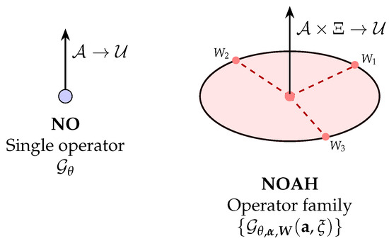
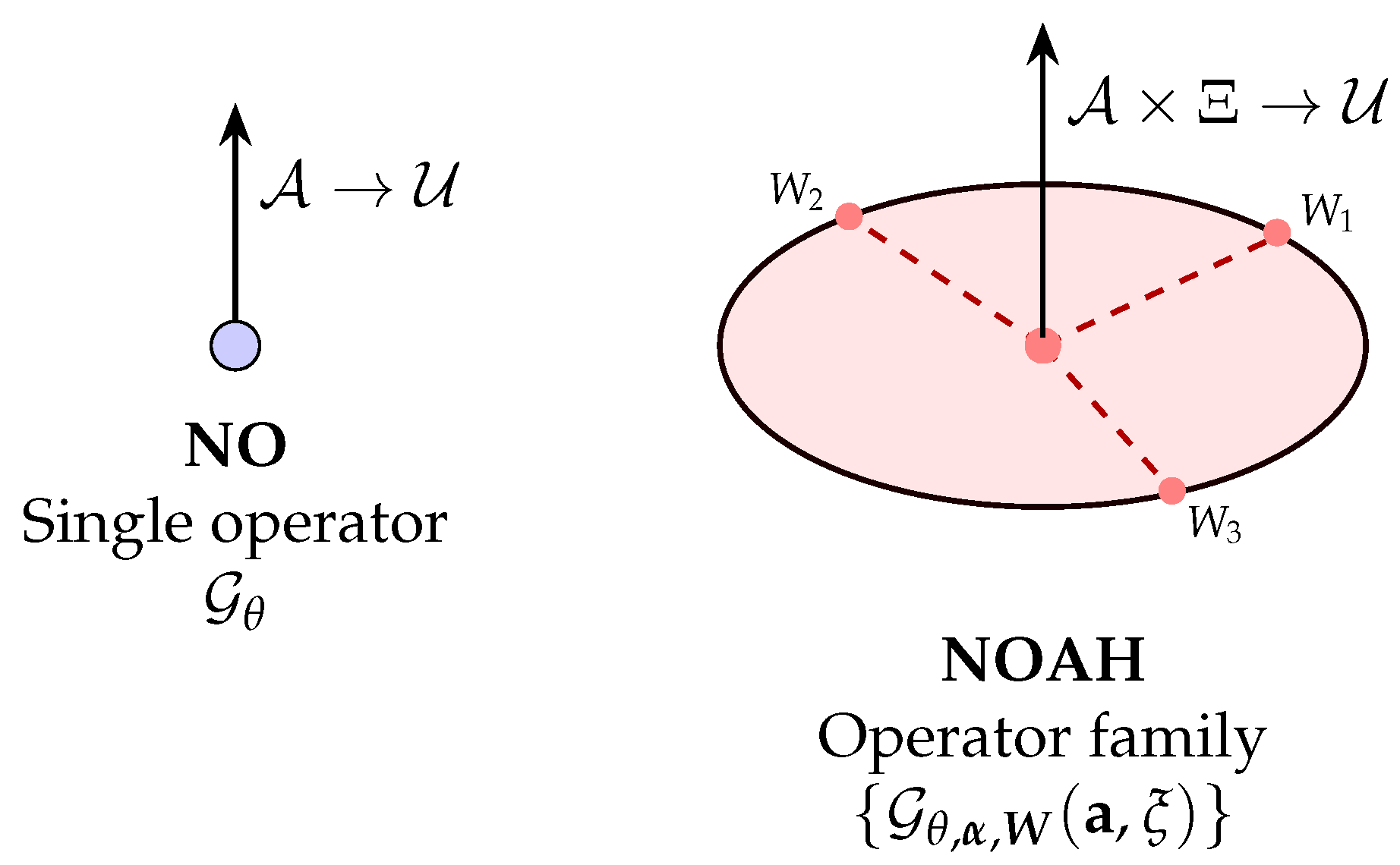
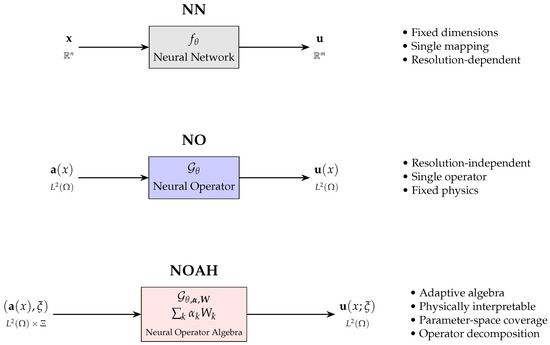
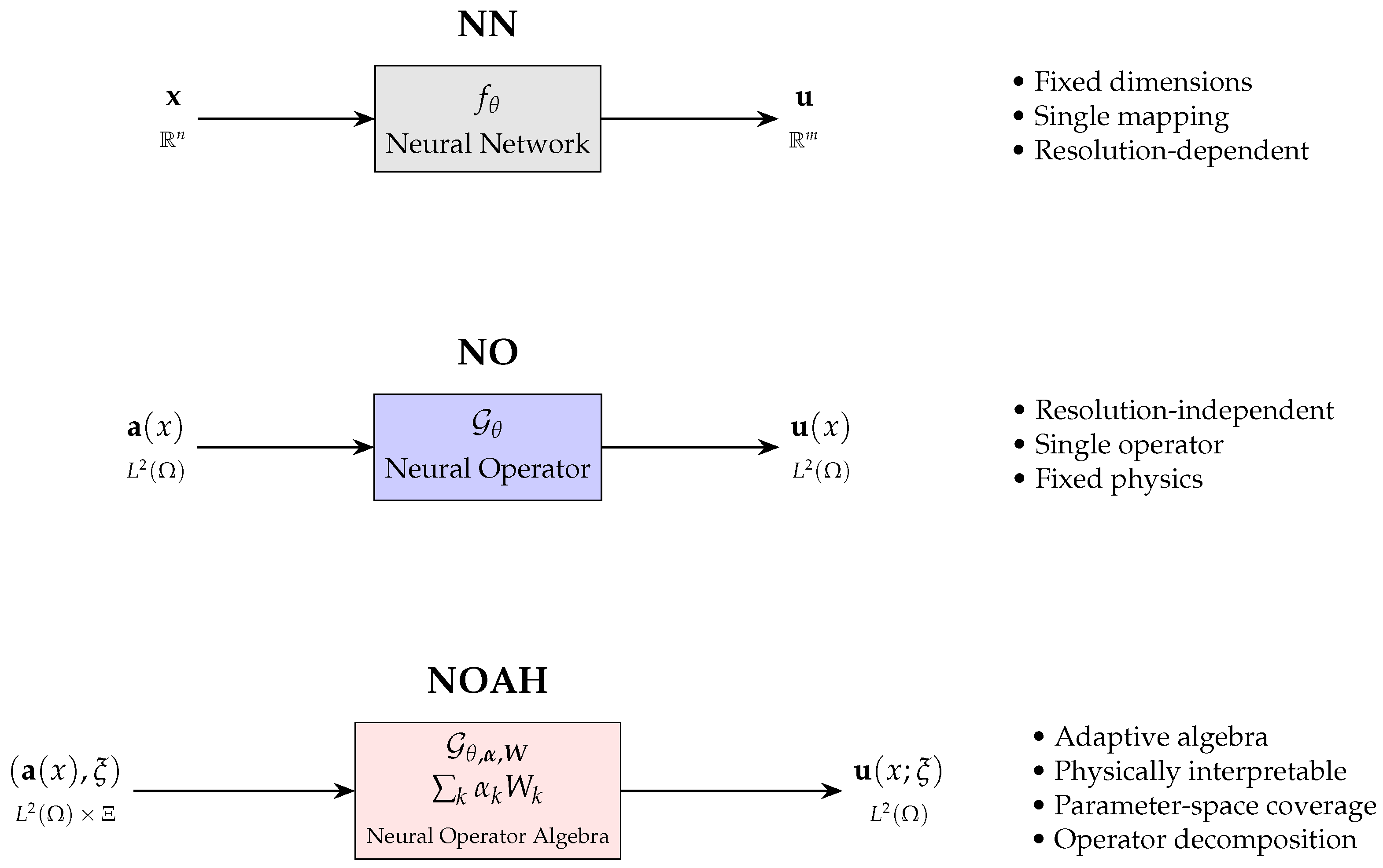
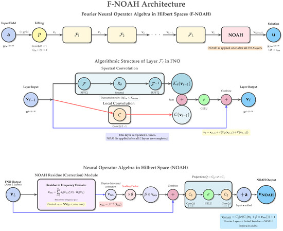
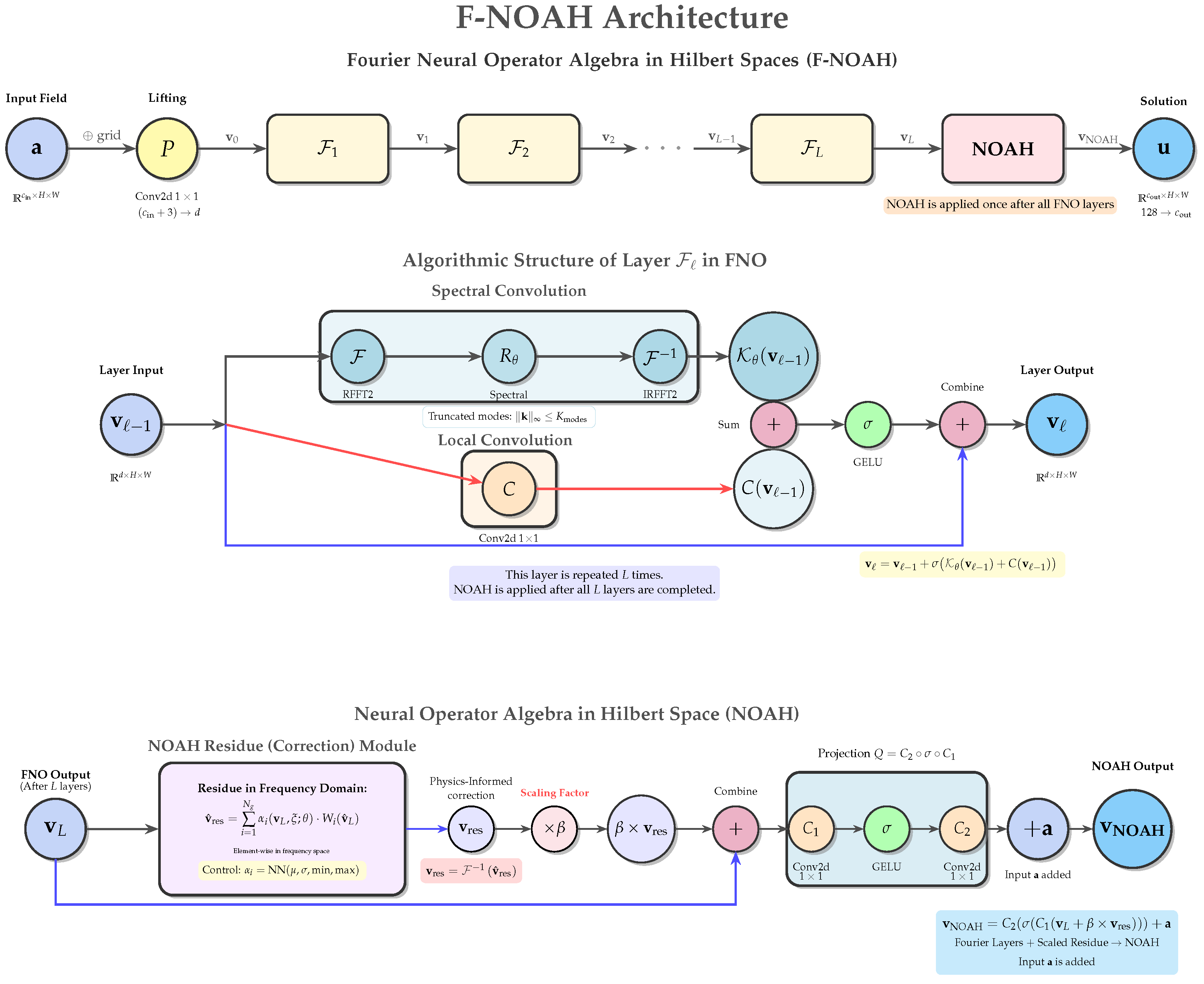
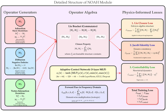
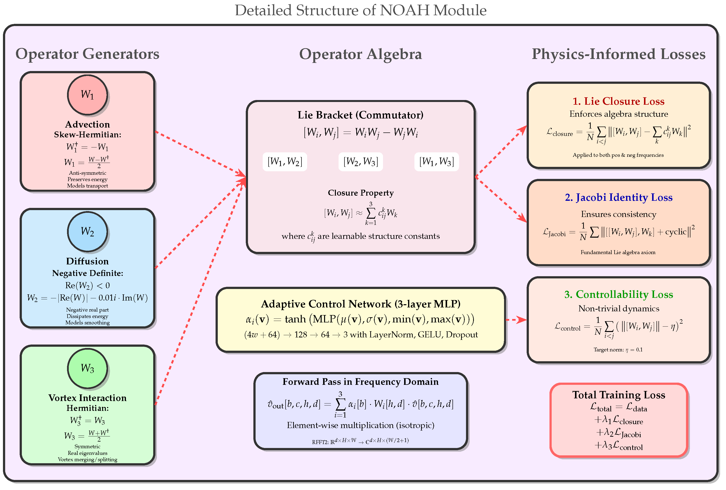
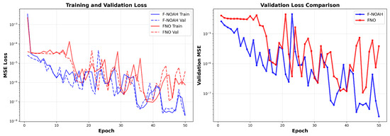
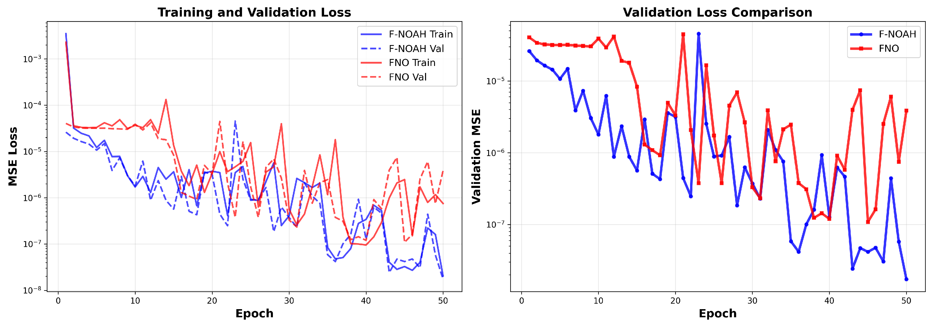
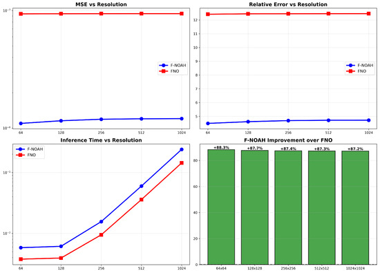
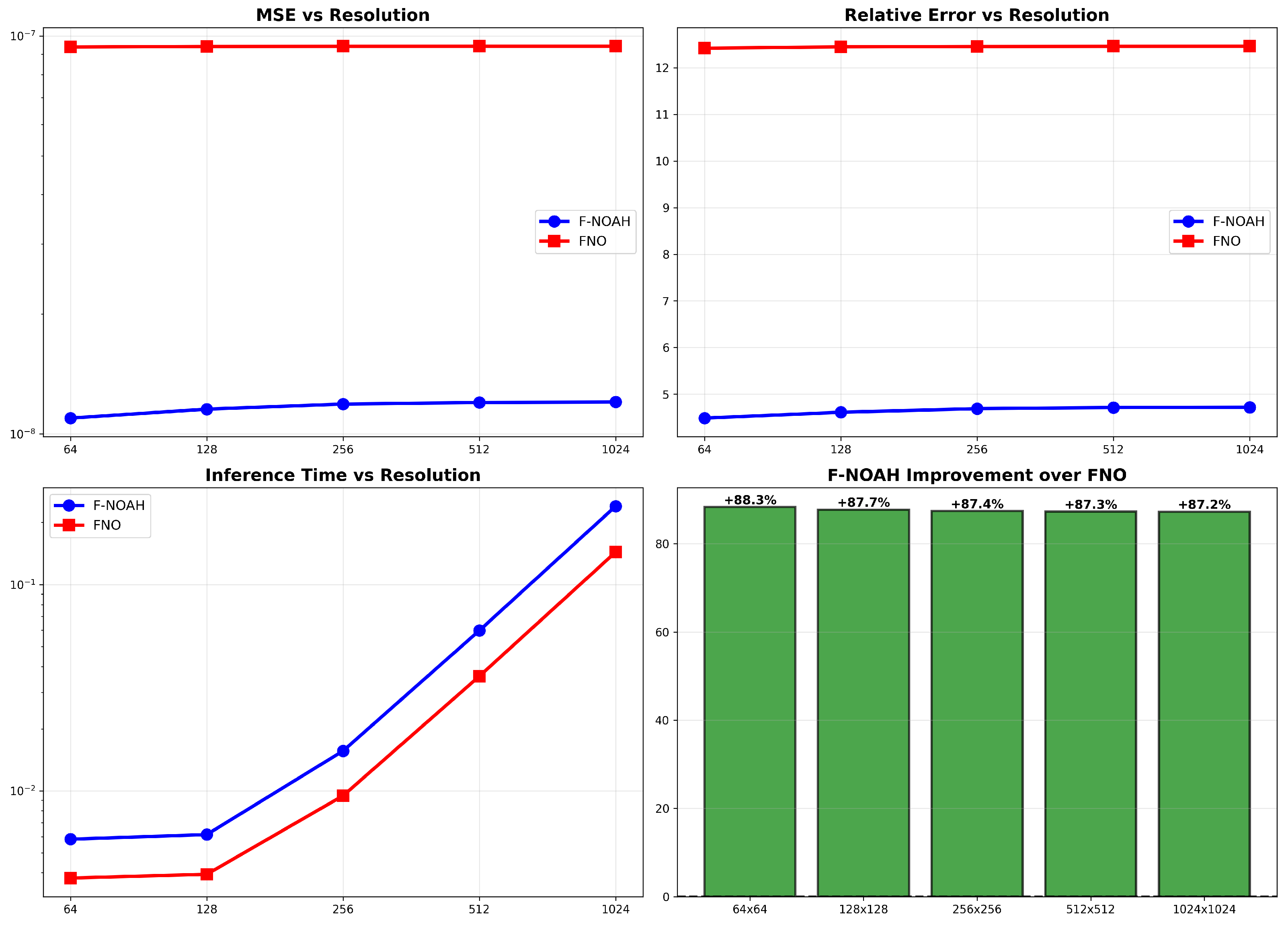
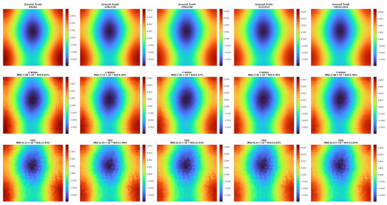
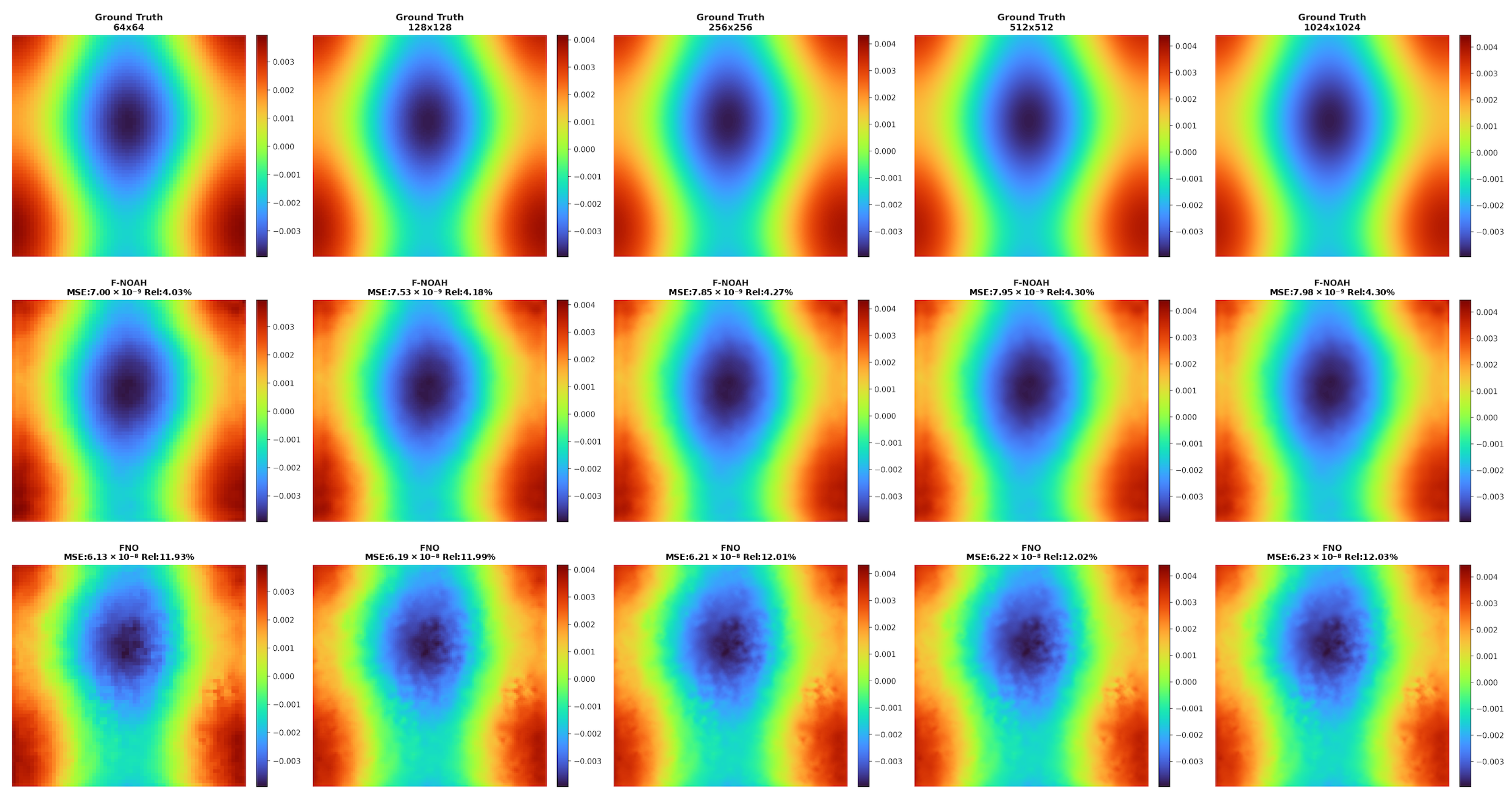
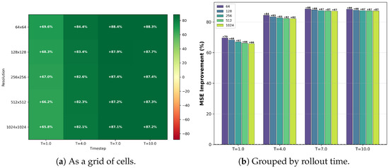
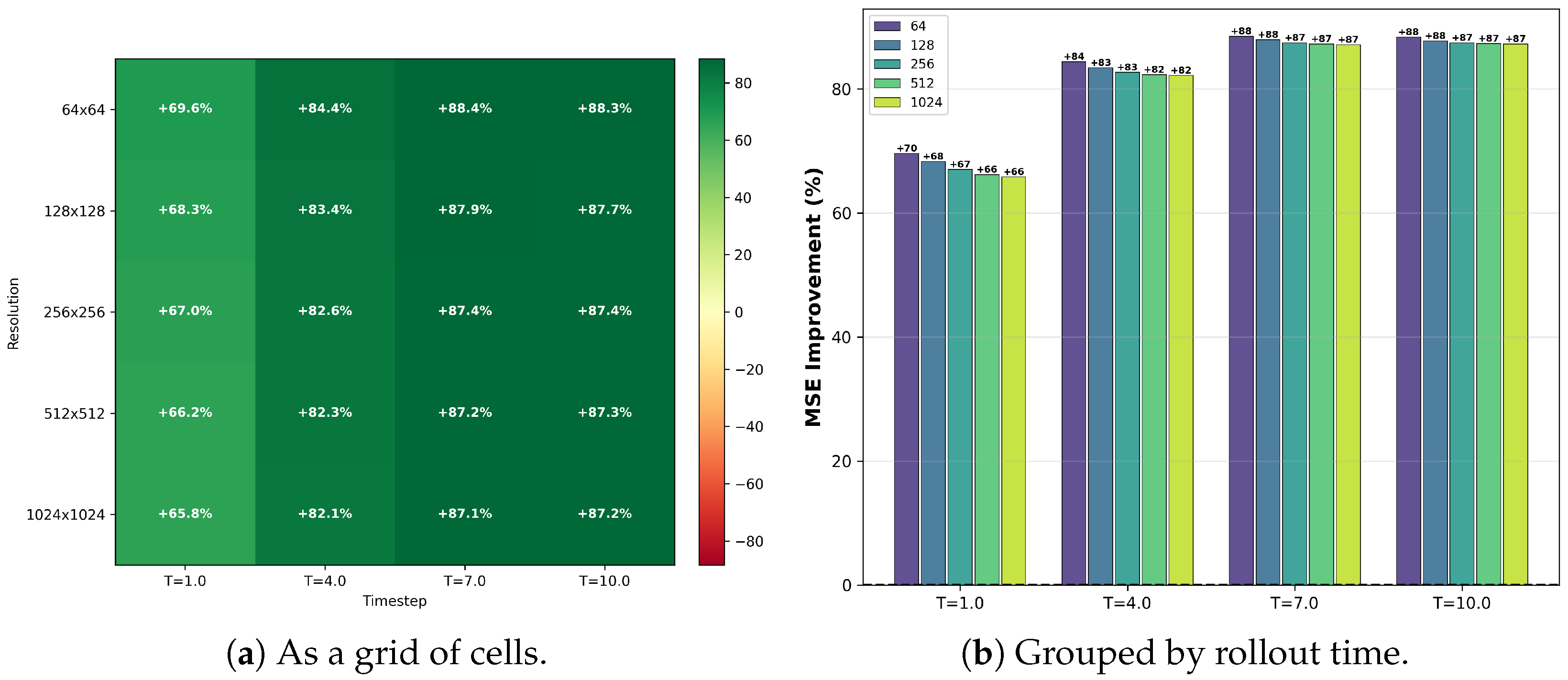
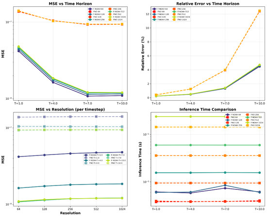
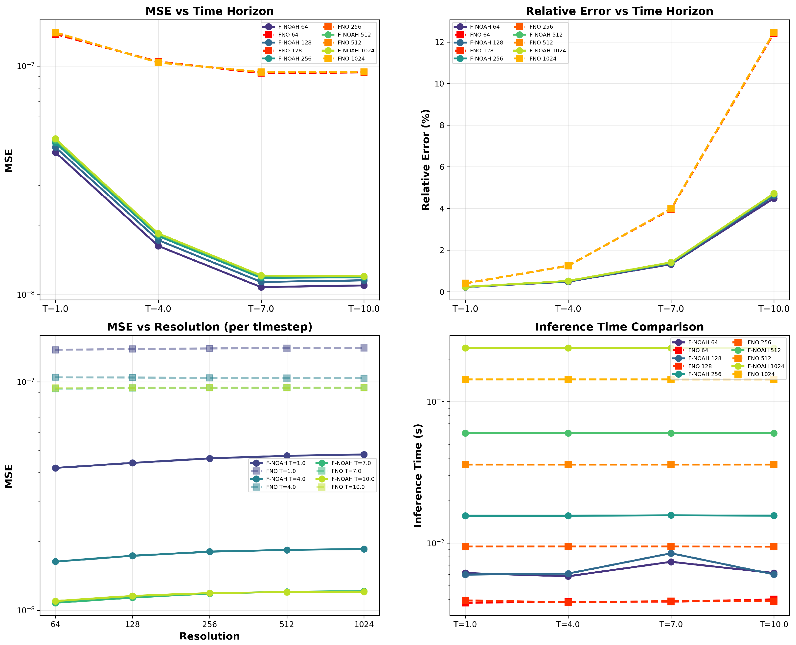
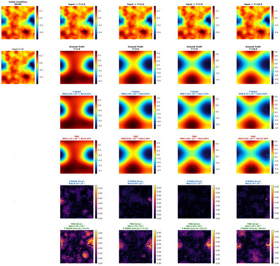
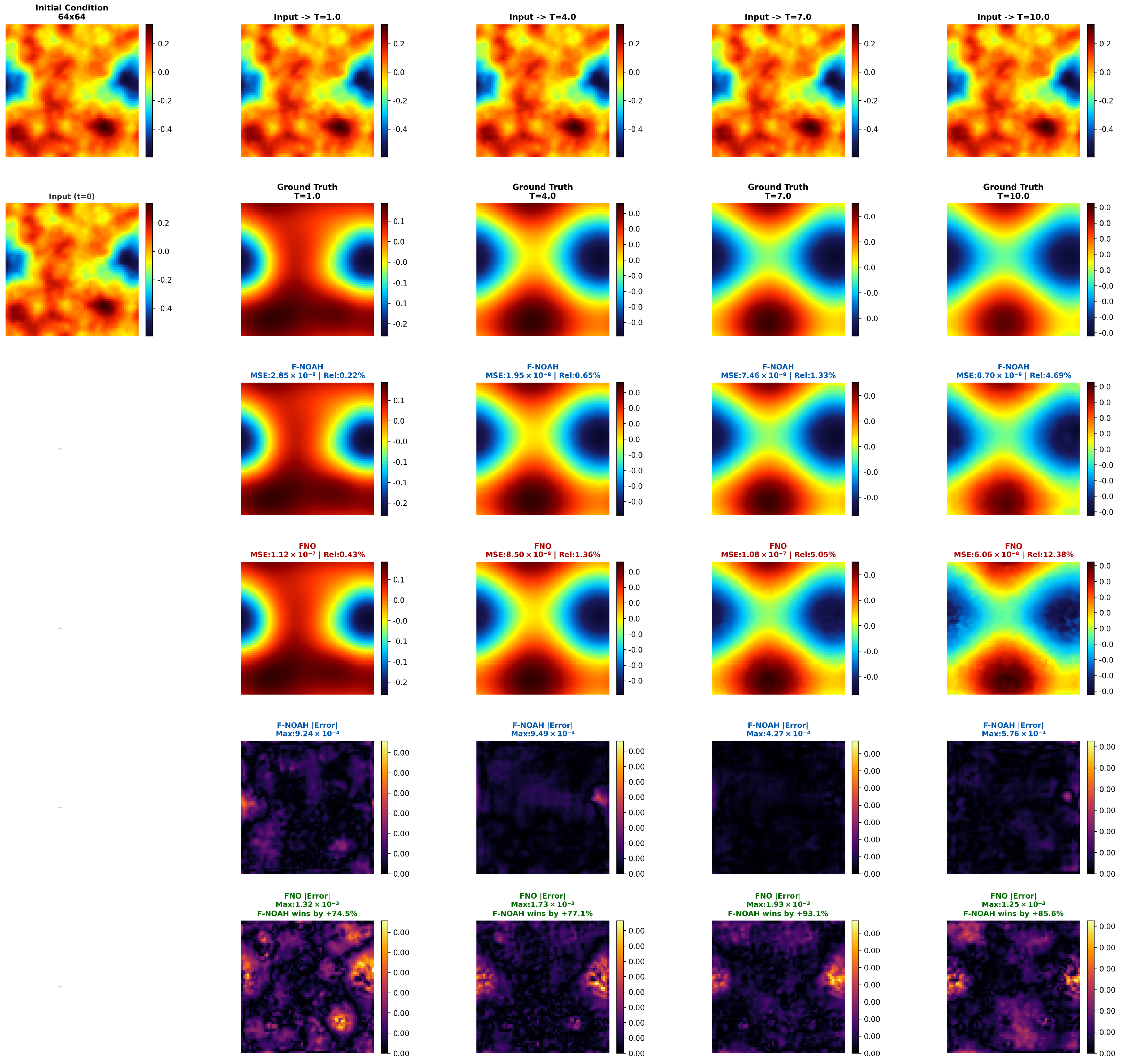
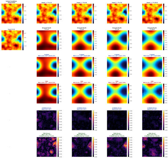
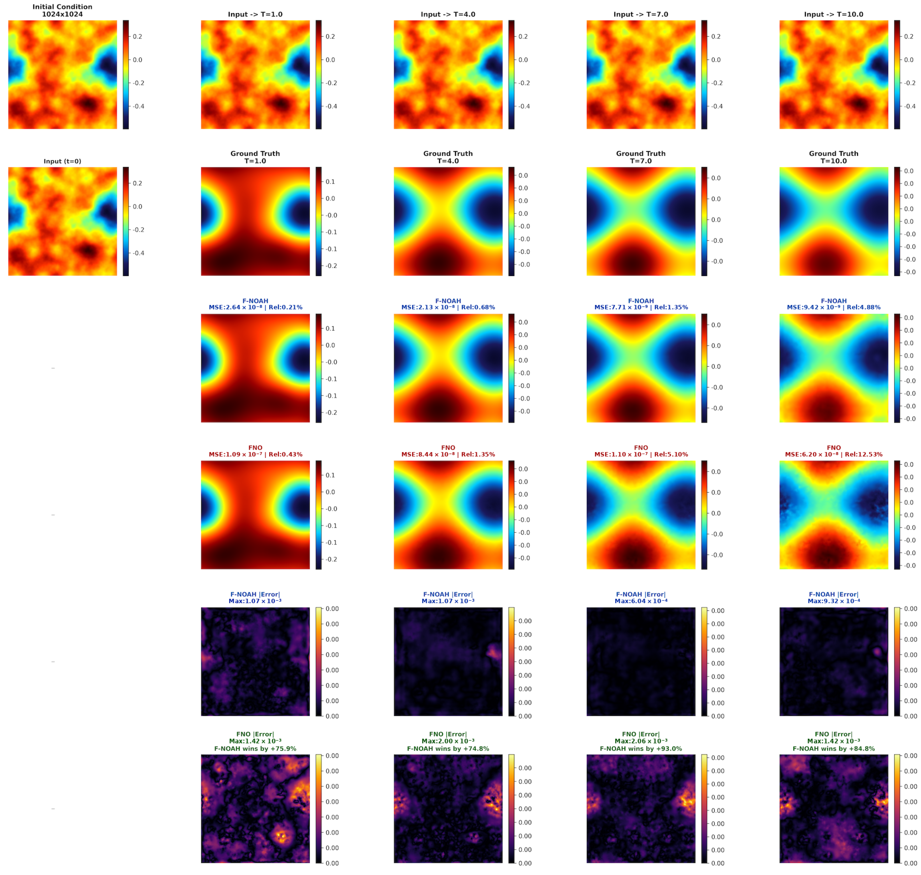
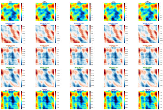
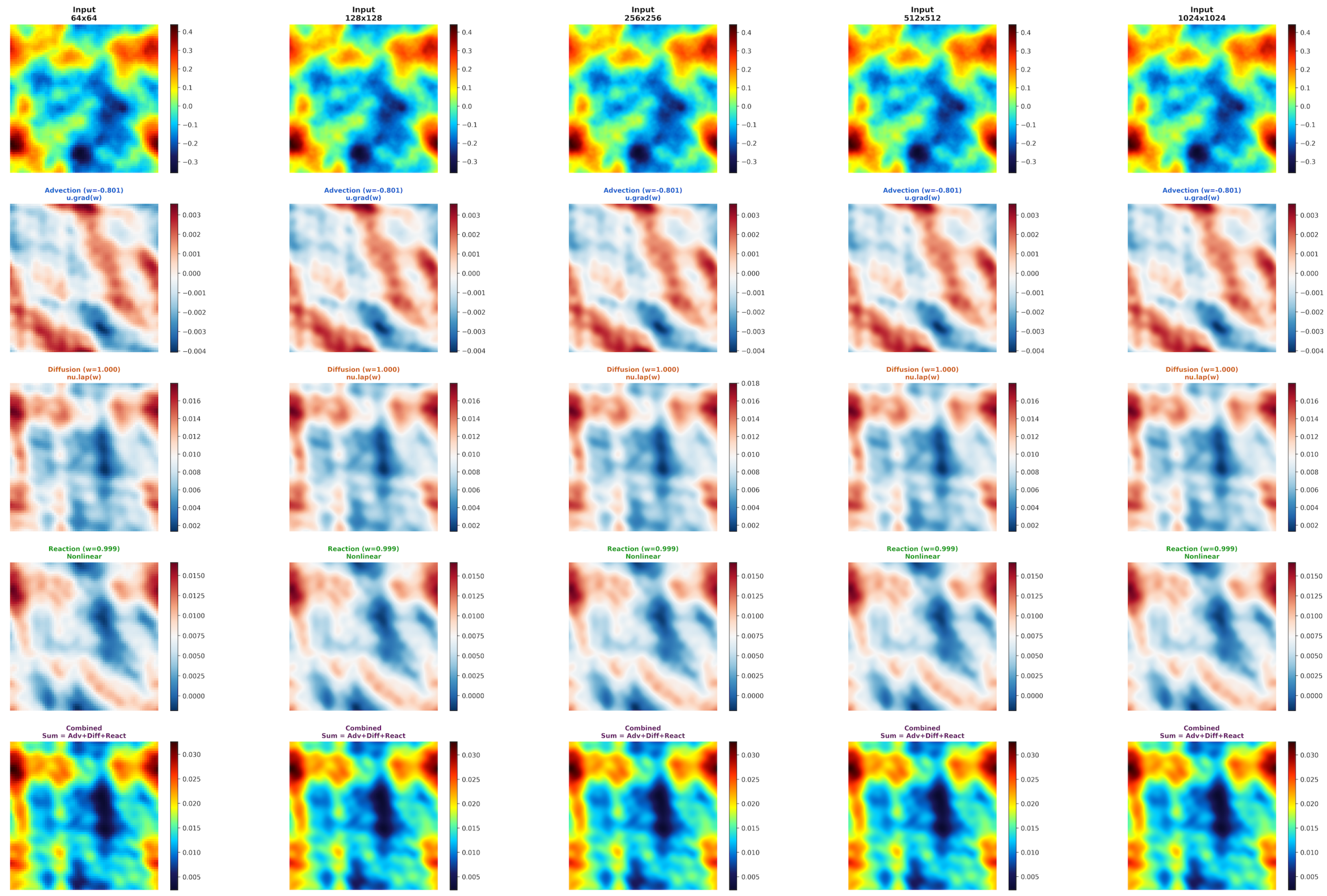
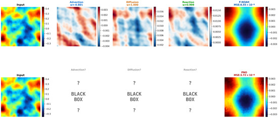
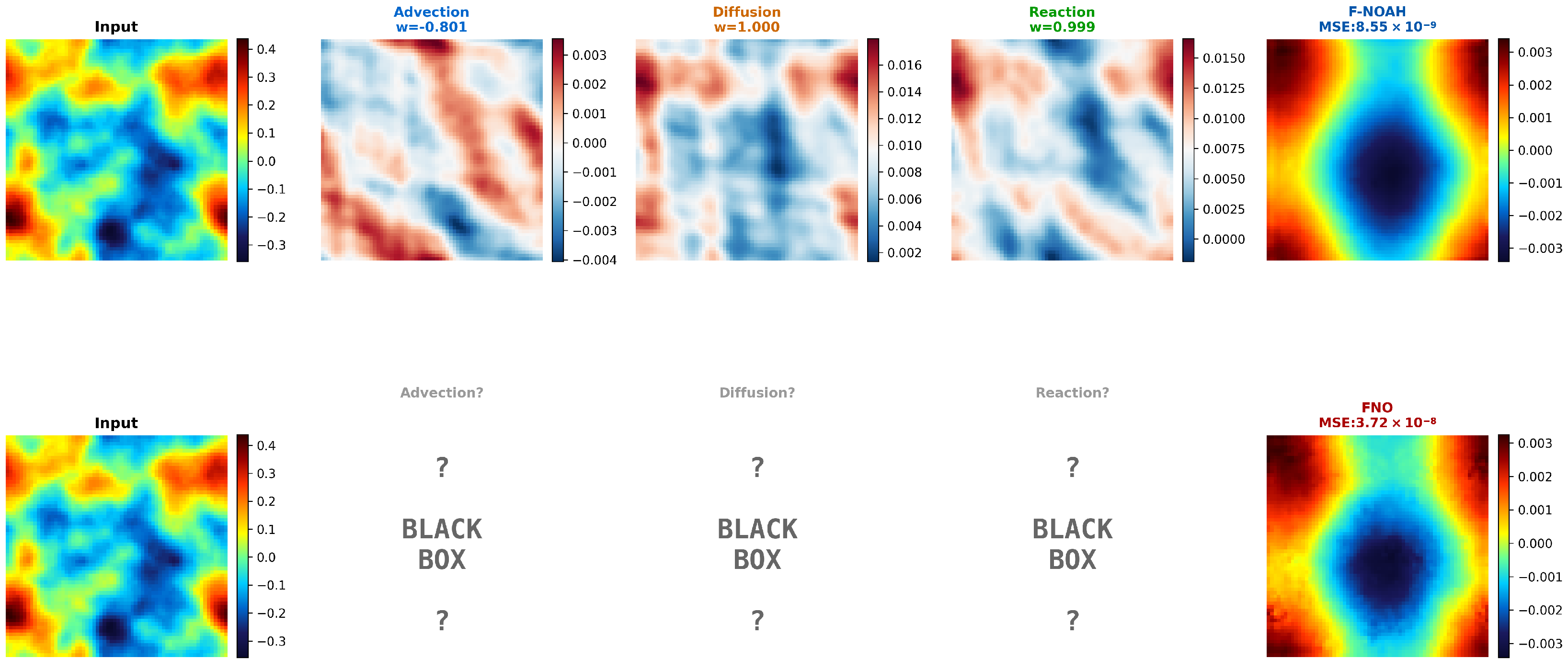
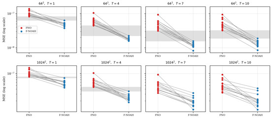
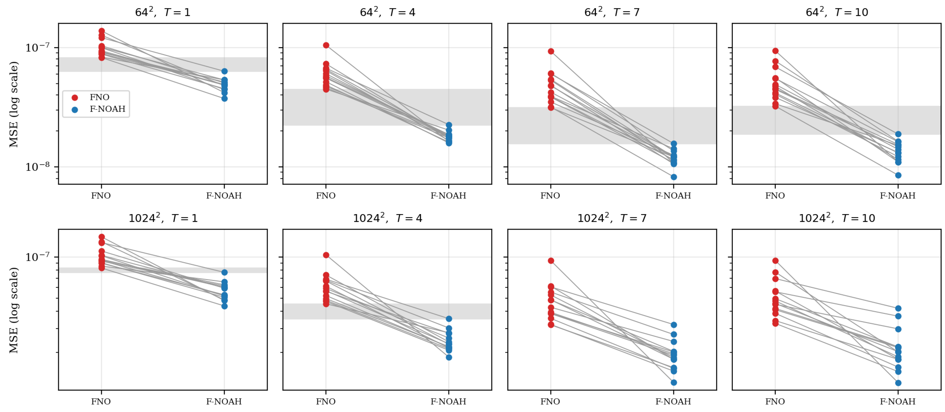
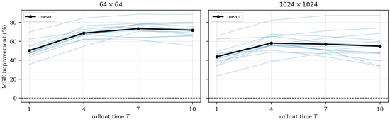
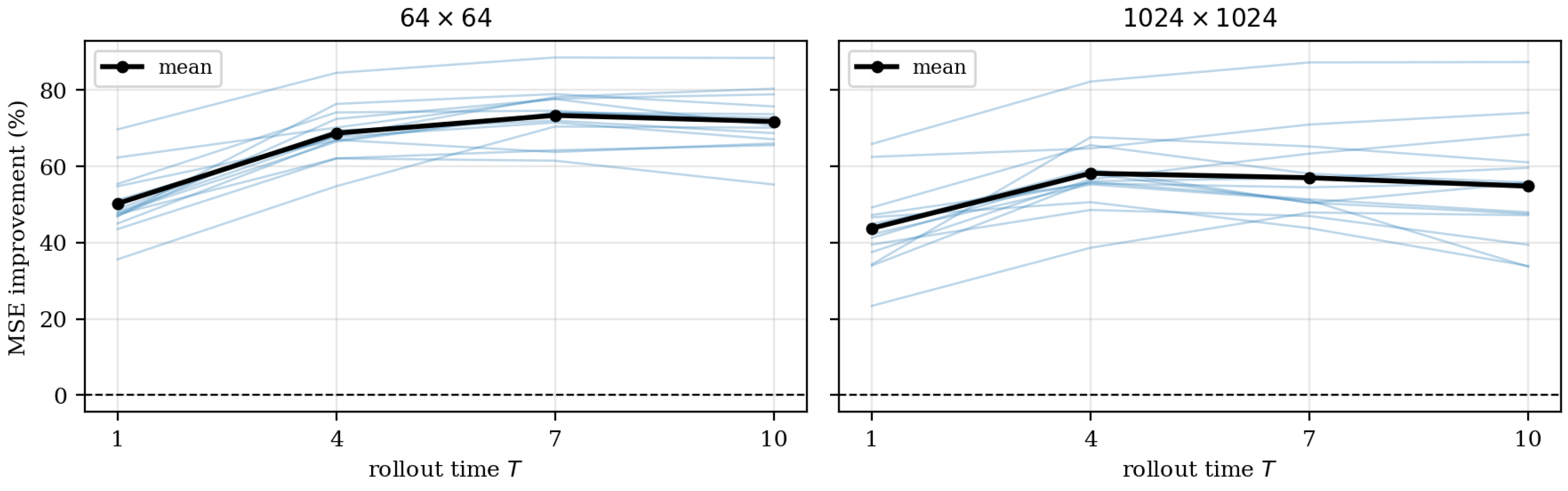
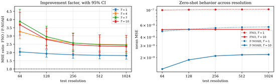
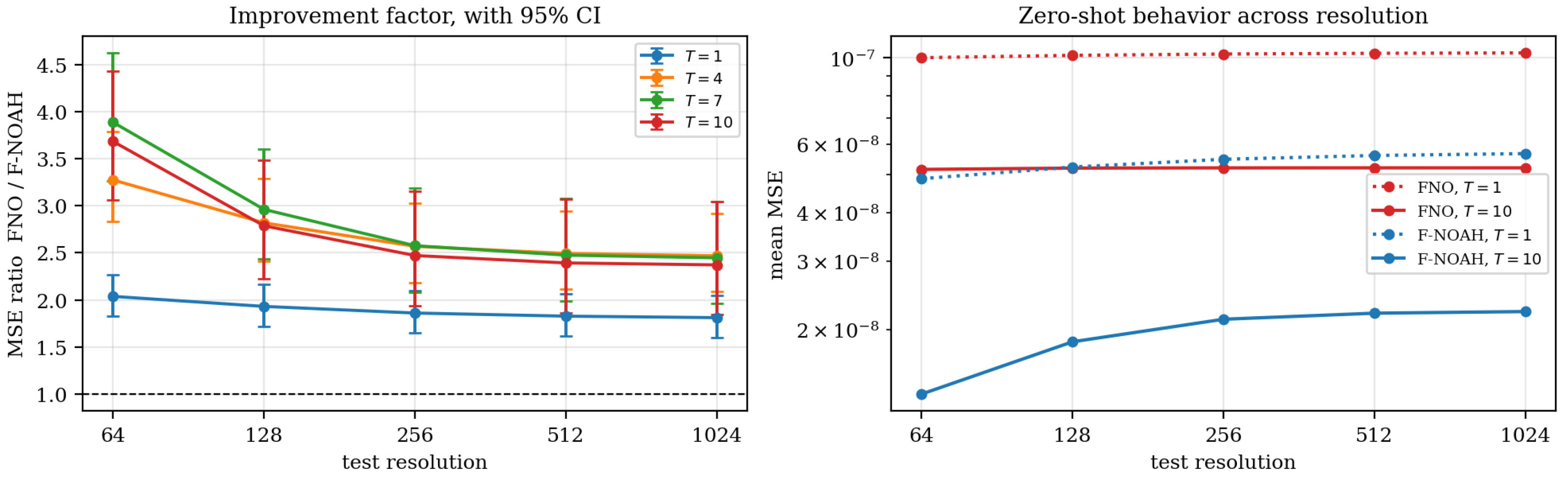
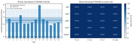
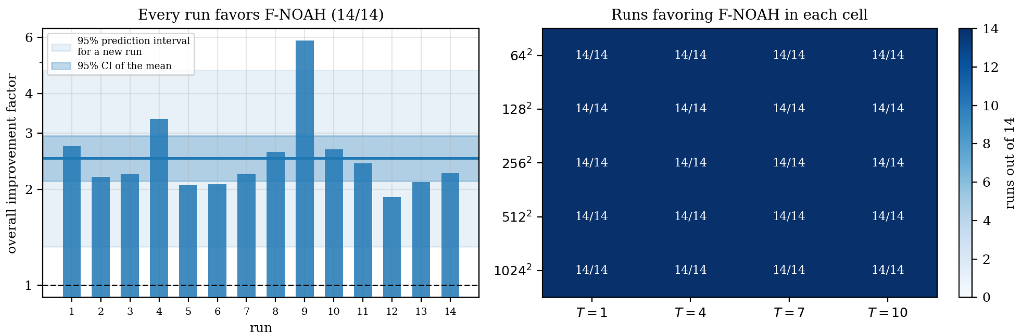

Disclaimer/Publisher’s Note: The statements, opinions and data contained in all publications are solely those of the individual author(s) and contributor(s) and not of MDPI and/or the editor(s). MDPI and/or the editor(s) disclaim responsibility for any injury to people or property resulting from any ideas, methods, instructions or products referred to in the content. |
© 2026 by the authors. Licensee MDPI, Basel, Switzerland. This article is an open access article distributed under the terms and conditions of the Creative Commons Attribution (CC BY) license.