


Abstract
Reliable wearable motion tracking depends not only on nominal sensor precision but on whether calibration remains valid after re-donning, anatomical misalignment, magnetic disturbance, temperature change, and prolonged operation. This structured critical review treats calibration as a system-level engineering decision spanning intrinsic inertial measurement unit (IMU) correction, sensor-to-segment alignment, flexible-sensor calibration, drift management, and complementary or external references. A reproducible Scopus core search conducted in May 2026 identified 807 records. Three co-authors screened titles, abstracts, and keywords using explicit eligibility criteria, with full-text inspection when required; the final 110-source reference corpus combines eligible core records with supplementary and contextual sources identified through coverage checks in IEEE Xplore, Web of Science, ScienceDirect, and the MDPI database. Unlike prior reviews that mainly treat individual calibration layers or inertial-error mechanisms, this review jointly compares sensor-level, anatomical, multimodal, adaptive, and external-reference routes within a common deployment-oriented framework. Evidence is coded by failure mechanism, calibration route, sensing modality, application context, validation context, and deployment constraint. No universally superior route is supported: static and functional alignment differ in burden and anatomical sensitivity; magnetometer use depends on field reliability; vision and ultra-wideband (UWB) references can restore absolute observability but add infrastructure dependence; and direct IMU–flex calibration remains comparatively sparse. The resulting decision framework prioritizes reproducibility, robustness, calibration stability, and fitness for real-world deployment over isolated best-case accuracy.
1. Introduction
1.1. Calibration as a Reliability Bottleneck in Wearable Electronics
The practical value of a wearable motion-sensing system is determined by the stability of its measurement chain after deployment, not only by the nominal specifications of its sensors. IMUs, flexible sensing elements, and multimodal wearable nodes are now used in rehabilitation, biomechanics, sports, industrial human–robot interaction, and mobile human–machine interfaces, where repeated donning, variable attachment, environmental interference, and long recording periods are routine rather than exceptional conditions [1,2,3,4,5,6]. Under these conditions, a calibration procedure that performs well in a controlled laboratory may not preserve the same accuracy once the sensing system is moved to everyday use.
Calibration must therefore be treated as a lifecycle function of the sensing system rather than a one-time preprocessing task. Intrinsic parameters, anatomical alignment, sensor attachment, magnetic conditions, temperature, motion dynamics, and the availability of external references can all alter the measurement model after deployment. A method that performs well in a short laboratory trial may consequently be unsuitable for an autonomous wearable operating for hours in an uncontrolled environment.
1.2. From Fragmented Calibration Methods to Application-Oriented Selection
Calibration errors arise at different levels of a wearable measurement chain. Bias and scale-factor errors distort the raw sensor output; frame and sensor-to-segment misalignment rotate measurements into incorrect anatomical coordinates; stochastic errors accumulate during integration; and environmental or mounting disturbances can invalidate parameters that were correct at the start of a session [7,8,9,10,11,12,13]. These mechanisms cannot be addressed by a single calibration operation.
The review literature represented in the present corpus is strongest for intrinsic calibration of microelectromechanical systems (MEMS)-based IMUs and inertial error modeling [14,15,16,17], with additional application-oriented reviews of wearable inertial sensing [3,5,18]. These syntheses are valuable, but they do not jointly compare, under the same deployment criteria, intrinsic sensor calibration, sensor-to-segment alignment, flexible-sensor nonlinearity and hysteresis, direct IMU–flex cross-modal calibration, adaptive or re-donning-aware recalibration, and external-reference routes based on vision or UWB. The novelty of the present review is therefore not another catalogue of calibration algorithms; it is a cross-layer engineering synthesis that links failure mechanisms to method selection through common constraints: observability, calibration burden, environmental sensitivity, infrastructure, operating duration, computational/power cost, and maturity of validation evidence.
IMUs and flexible sensors are considered together here because they expose complementary calibration problems, not because direct IMU–flex calibration already constitutes a mature standalone field. IMUs provide high-bandwidth inertial information but remain vulnerable to integration drift, magnetic disturbance, and frame-alignment errors; flexible sensors provide local deformation information without numerical integration but introduce nonlinearity, hysteresis, mounting dependence, and cross-joint coupling [2,19,20]. Direct cross-modal calibration is consequently treated as an emerging multisensor route within a broader calibration landscape. In this review, reliability is used as the deployment-level ability to preserve valid tracking performance under relevant operating conditions. To avoid conflating distinct performance concepts, Table 1 separates the five terms most frequently used in the comparative synthesis.
Table 1.
Operational distinctions among core performance terms used in this review.
The purpose of this review is to connect dominant failure mechanisms with defensible calibration choices. Four questions organize the synthesis: (RQ1) which calibration-relevant error mechanisms are represented in the literature; (RQ2) which sensor-level, anatomical, adaptive, multisensor, and external-reference routes are used to address them; (RQ3) how do validation context, infrastructure, magnetic conditions, calibration burden, and operating duration alter method selection; and (RQ4) where is the evidence sufficiently mature to support practical guidance and where should conclusions remain cautious?
The remainder of the paper follows an engineering decision sequence. Section 2 defines the review protocol and evidence base; Section 3 identifies failure modes that determine calibration requirements; Section 4 compares calibration and error-compensation routes; Section 5 converts the evidence into application-specific selection rules; Section 6 discusses design conflicts, evidence maturity, and research priorities; and Section 7 summarizes the resulting engineering guidance.
2. Review Approach and Evidence Base
This review uses a structured critical-review design to compare calibration choices across heterogeneous wearable-motion applications. Its purpose is not to estimate a pooled treatment effect. Traceability is instead supported by a reproducible core search, explicit eligibility rules, independent screening, structured evidence coding, and claim-specific interpretation of evidence strength.
2.1. Structured Search and Eligibility Criteria
The structured core search was executed in Scopus in May 2026 because of its broad coverage of engineering, instrumentation, computer science, and biomechanics. The search combined three concept blocks: wearable human-motion applications, calibration or compensation processes, and sensing modalities. The exact Scopus query was TITLE-ABS-KEY((“wearable” OR “motion capture” OR “human motion tracking” OR “human–machine interface” OR “HMI”) AND (“calibration” OR “drift compensation” OR “sensor fusion”) AND (“IMU” OR “inertial measurement unit” OR “flex sensor” OR “flexible sensor” OR “resistive flex sensor”)). With document type restricted to journal articles and conference papers, the Scopus search returned 807 records. The detailed review emphasized publications from 2015 to May 2026, while earlier foundational studies were retained when necessary to explain established calibration principles.
IEEE Xplore, Web of Science, ScienceDirect, and the MDPI database were used as complementary coverage checks rather than as independent bibliometric datasets. For reproducibility, the same three Boolean concept blocks were applied in each interface using its closest equivalent of title/abstract/keyword or topic/all-metadata search fields: (wearable OR “motion capture” OR “human motion tracking” OR “human–machine interface” OR HMI) AND (calibration OR “drift compensation” OR “sensor fusion”) AND (IMU OR “inertial measurement unit” OR “flex sensor” OR “flexible sensor” OR “resistive flex sensor”). The detailed review emphasized 2015 to May 2026, while earlier foundational studies were retained when required to explain established calibration mechanisms. Database-specific result counts for these supplementary coverage checks were not preserved in the archived review materials, so a combined five-database retrieval count is not retrospectively reconstructed. This distinction is important: the 807-record Scopus set is the original May 2026 bibliometric core dataset, whereas the other databases were used to reduce coverage gaps and identify additional relevant or contextual sources.
2.2. Screening and Reference Corpus
All 807 records in the Scopus core set were assessed using title, abstract, and keywords, with full-text inspection when relevance could not be determined from bibliographic information alone. Eligible publications addressed wearable human-motion sensing and at least one calibration-relevant problem, including intrinsic sensor errors, sensor-to-segment alignment, drift compensation, sensor fusion, flexible-sensor calibration, temporal synchronization, or multisensor calibration. Non-wearable navigation studies were retained only when they provided transferable calibration methodology or foundational evidence on physical error mechanisms. Material- or device-only flexible-electronics studies without motion-calibration relevance, non-human applications without transferable methodology, activity-recognition or classification studies without a calibration or motion-reconstruction contribution, non-peer-reviewed material, duplicates, and sources lacking sufficient methodological information were not retained in the calibration-focused evidence corpus.
Three co-authors screened the Scopus core using the same eligibility criteria, and borderline records were resolved by consensus. Sources identified through the complementary coverage checks in IEEE Xplore, Web of Science, ScienceDirect, and the MDPI database were assessed using the same relevance logic and reconciled against the existing reference corpus to avoid duplicate citation of the same study. These complementary databases were used to improve topical coverage rather than to define a pooled five-database bibliometric denominator.
To improve source-level traceability, a record-level provenance audit was performed between the 807-record Scopus core dataset and the final 110-reference manuscript corpus. Matching used exact DOI correspondence where available, followed by normalized publication-title matching. The audit identified 23 final references directly retrieved by the Scopus core query. Consequently, 784 records from the Scopus core are not represented in the final manuscript reference corpus. No duplicate DOI records were identified within the audited 807-record Scopus dataset. The remaining 87 references in the final corpus were not directly retrieved by the core Scopus query and represent complementary, contextual, or foundational sources identified through the additional database coverage or retained to support transferable calibration principles.
The 784 Scopus-core records not represented in the final corpus should not be interpreted as a single-stage title/abstract exclusion count. The original review workflow did not archive separate numerical counters for title/abstract exclusions, subsequent full-text exclusions, or database-of-first-discovery counts for supplementary sources. Because this study was designed as a structured critical review rather than as a prospectively registered systematic review, these unrecorded stage-specific values were not retrospectively reconstructed. Figure 1 therefore presents a PRISMA-style transparency flow that reports only verifiable counts while making the screening logic, complementary-source role, and final corpus assembly explicit.
Figure 1.
PRISMA-style flow diagram of literature identification, screening, eligibility assessment, and construction of the final reference corpus. Dashed arrows indicate the complementary/manual coverage pathway (sources identified outside the core Scopus query), as distinct from the solid-line systematic screening pathway.
2.3. Evidence Coding and Interpretation
During synthesis, each source received non-exclusive codes for sensing modality, calibration or error domain, application context, validation/reference context, deployment constraints, and its role in the review. Deployment codes captured factors that materially affect engineering selection, including infrastructure dependence, magnetic environment, re-donning sensitivity, operating duration, and computational or power burden. Multiple labels were allowed because one source can support more than one calibration problem.
Strength of support is interpreted at the level of individual claims rather than through a single numerical quality score across non-equivalent study designs. Greater weight is given to conclusions supported by multiple independent studies, quantitative validation against an external or clearly defined reference, realistic movement conditions, and longer or repeated testing. Findings supported mainly by proof-of-concept or sparsely replicated studies are explicitly described as emerging. The ‘first-line’ routes in the deployment-oriented comparison tables presented in Section 4 were derived from this coding: a route is presented as first-line only when it directly addresses the dominant failure mechanism for the stated application and is supported by convergent evidence from multiple studies or by repeated application-level validation. Where direct evidence is limited, the tables use qualified language such as ‘candidate’, ‘emerging’, or ‘limited direct evidence’ rather than implying a universal recommendation.
2.4. Database Coverage, Bias, and Reproducibility Limits
Database coverage is not interchangeable. Scopus provides broad multidisciplinary indexing and a substantial conference-paper component; IEEE Xplore is especially strong in engineering conference and standards-adjacent literature; Web of Science is more selective and journal-oriented; ScienceDirect is publisher-specific; and the MDPI database is publisher-specific. The supplementary databases were therefore used to check topical coverage rather than to create a single pooled bibliometric denominator. The documented core query contains no language term, but the accessible literature and the final corpus are dominated by English-language sources, so language-access bias cannot be excluded.
Further review-level biases are also relevant. Positive or successful calibration results are more likely to be published than null or negative findings; methods supported by widely used benchmark datasets may be overrepresented; short conference papers can provide less complete validation detail than full journal articles; and emerging methods may appear promising because they have been tested by only a small number of groups. These limitations are explicitly considered when using terms such as ‘promising’, ‘emerging’, or ‘well established’ and when formulating the application-oriented recommendations in Section 5.
2.5. Descriptive Scope and Bibliometric Context
Figure 2, Figure 3, Figure 4, Figure 5 and Figure 6 provide descriptive context for the original May 2026 807-record Scopus core query by showing publication output, geographic distribution, document type, subject area, and leading source titles. These plots are used only to characterize the search landscape and are not interpreted as evidence of calibration effectiveness. Figure 7 provides a keyword co-occurrence map used as a topical scope check. Retaining these plots makes the composition and disciplinary coverage of the core dataset transparent, while the method-selection conclusions in Section 4, Section 5 and Section 6 are based on the source-level qualitative synthesis rather than bibliometric frequency.
Figure 2.
Annual publication output returned by the Scopus core query (807 records). The 2026 value is partial because the search was conducted in May 2026. Source: Scopus (Elsevier), Analyze Results.
Figure 3.
Top ten countries/territories represented in the Scopus core-query results. Source: Scopus (Elsevier), Analyze Results.
Figure 4.
Distribution of document types in the Scopus core-query results. Source: Scopus (Elsevier), Analyze Results.
Figure 5.
Distribution of subject areas in the Scopus core-query results. Source: Scopus (Elsevier), Analyze Results.
Figure 6.
Annual publication output for the five most represented source titles in the Scopus core-query results. Source: Scopus (Elsevier), Analyze Results.
Figure 7.
Keyword co-occurrence network derived from the Scopus core-search export using VOSviewer 1.6.21 (full counting). Node size represents occurrence frequency, node color indicates cluster membership, and edge thickness represents co-occurrence strength. Source: authors’ analysis of the Scopus export.
The temporal profile is descriptive and shows increased publication activity in the later years of the search window, particularly after 2019. No causal analysis was performed, so the trend is not attributed here to COVID-19 restrictions, artificial-intelligence adoption, or any other specific driver. The 2026 count is necessarily partial because the original Scopus search was performed in May 2026.
The record-count distribution is descriptively led by China and the United States, followed by contributions from several European and Asian countries. No inferential statistical test was applied to country differences; Figure 3 is a descriptive ranking of Scopus record counts rather than evidence of a statistically significant geographic effect.
Journal articles and conference papers account for the great majority of the retrieved records, whereas review papers constitute only a small share of the dataset. The document-type profile is therefore used here only to describe the structure of the search corpus.
Engineering and computer science constitute the largest subject-area contributions, with additional representation from biomedical, medical, physical, and materials-related fields. This breadth reflects the combined sensor, algorithmic, and human-motion focus of the literature.
The leading source titles similarly span sensor engineering, instrumentation, and biomechanics. Keyword co-occurrence was therefore examined separately to characterize the internal thematic structure of this multidisciplinary corpus (Figure 7).
The map is used only as a descriptive scope check. It indicates that inertial and flexible sensing are connected within the wearable-motion literature but does not establish a mature joint IMU–flex calibration field. The review therefore evaluates direct IMU–flex work as one emerging multisensor route and places it alongside better-established IMU, sensor-to-segment, adaptive, and external-reference strategies.
3. Calibration Failure Modes in Wearable Motion Tracking
The relevant question for calibration design is not simply which sensor is used but which failure mechanism remains observable and correctable during operation. The error evidence is therefore organized by correction requirement: intrinsic deterministic errors that can be identified through calibration, stochastic errors that require dynamic compensation, and context-dependent disturbances that can invalidate an otherwise correct calibration (Figure 8).
Figure 8.
Calibration-relevant failure modes in wearable motion sensing, grouped into systematic (deterministic) errors, random/stochastic errors, and environmental disturbances. The categories overlap in practice because environmental and mounting effects can modify intrinsic parameters and propagate into orientation and joint-angle estimates. Source: authors’ own elaboration. Dashed arrows indicate the combined, overlapping contribution of all three error categories to the downstream impact on orientation, joint-angle estimation, drift, and motion reconstruction, as distinct from the solid arrows above, which denote categorical decomposition.
Where quantitative examples are drawn from navigation or other non-wearable inertial studies, they are used only to illustrate transferable physical error mechanisms and calibration principles; their numerical performance should not be interpreted as directly transferable to wearable joint-angle accuracy or deployment performance.
3.1. Intrinsic Errors Addressable by Sensor-Level Calibration
Systematic errors represent deterministic deviations from true values that remain consistent under fixed conditions and are typically associated with sensor imperfections such as bias, scale factor errors, and axis misalignment arising from manufacturing limitations and calibration inaccuracies. In addition, these deterministic errors propagate through integration processes, contributing to drift in orientation and position estimates during operation [21,22,23].
3.1.1. Bias and Bias-Driven Drift
Bias errors are a major source of inaccuracy in inertial measurement units (IMUs), defined as constant or slowly varying offsets present even under zero input conditions. These errors may consist of a constant component and a time-varying drift influenced by factors such as temperature and stochastic processes [24]. Due to integration in inertial navigation systems, even small bias values lead to accumulating drift, particularly in orientation, which further propagates to velocity and position estimates. This effect is directly related to inaccuracies in angular rate measurements, which introduce errors in the numerical integration used for orientation estimation [25].
Unlike scale factor and misalignment errors, bias introduces systematic drift independent of motion dynamics, making it especially critical in both static and low-dynamic applications. Gyroscope bias is typically the dominant contributor to overall navigation error, and its compensation is essential for maintaining system accuracy.
Effective bias calibration significantly improves navigation performance, even when simple calibration procedures are applied [26]. For instance, the study in [26] demonstrated that a two-position calibration scheme completed in approximately 20.5 min can calibrate gyroscope bias on the order of 5 × 10⁻³°/h, improving position accuracy by 72.68% and heading accuracy by 79.65% over a 12-h navigation experiment [26]. Their comparative analysis further showed that gyro bias alone contributed a 6.75′ heading error over 24 h—substantially larger than the contribution from scale factor error (0.03′) or installation misalignment (2.08′)—confirming bias as the dominant error source in low-dynamic applications [26]. Recent studies also demonstrate that advanced data-driven methods, such as adaptive neuro-fuzzy inference system (ANFIS), can effectively estimate and compensate both bias and stochastic errors, leading to substantial improvements in navigation accuracy [27].
3.1.2. Scale-Factor and Gain Errors
Scale-factor error is a proportional gain deviation that propagates into integrated orientation estimates [25]. Even small uncorrected gains can matter during long operation: in the simulation reported in [26], a 0.01% error on the rapid-rotation axis produced 90 arc min of orientation error over 30 min, whereas periodic refinement reduced the error below 3.5 arc s. The example illustrates why scale-factor calibration remains relevant even when the nominal gain error appears small.
In modern inertial sensors, particularly high-performance MEMS gyroscopes, scale factor errors are often dominated by nonlinear effects rather than simple linear deviations. These nonlinearities arise from internal coupling mechanisms, such as parasitic capacitance, which introduce higher-order dependencies on angular rate and distort the sensor output characteristics [28].
Although scale factor errors are typically less dominant than bias in low-dynamic conditions, their impact increases significantly in dynamic scenarios, where motion-dependent effects amplify measurement inaccuracies. Therefore, accurate modeling and calibration of both linear and nonlinear components of scale factor errors are essential for ensuring high-precision navigation performance, particularly in advanced or high-speed applications [29].
3.1.3. Axis and Frame Misalignment
Axis misalignment errors arise from non-orthogonality and imperfect alignment between sensor axes, as well as from installation inaccuracies between different coordinate frames within the IMU [26,30]. These errors lead to cross-axis coupling, where motion along one axis produces spurious outputs in others, significantly degrading measurement accuracy.
The magnitude of this effect has been quantified experimentally: for a strapdown IMU with installation misalignment of 30 arcseconds on off-diagonal axis terms, a 24-h navigation simulation showed that gyroscope misalignment alone produced a heading error of 2.08′ and a position error of 4.34 km, while accelerometer misalignment produced a position error of 2.77 km—smaller than the corresponding contribution from bias error (26.27 km for gyro bias) but larger than the contribution from scale factor error alone (1.67 km) [26]. This confirms that, while less dominant than bias, installation misalignment remains a non-negligible contributor to overall system error, particularly under dynamic motion conditions where the coupling between misaligned axes and vigorous carrier motion amplifies the resulting error, as shown in Equations (9) and (10) of [26].
In practical systems, misalignment occurs at multiple levels, including internal sensor misalignment (e.g., between accelerometer and gyroscope frames) and installation errors between the IMU and the host platform or gimbal mechanism. These effects are commonly modeled using small-angle approximations, where misalignment is represented as a skew-symmetric perturbation of the identity transformation matrix [30].
Moreover, in wearable and biomechanical applications, sensor-to-segment misalignment has been shown to significantly affect the accuracy of joint angle estimation, highlighting the sensitivity of kinematic reconstruction to orientation errors [31].
Additionally, misalignment errors may evolve over time due to mechanical deformation, thermal effects, or mounting inaccuracies, making periodic calibration necessary to maintain system performance. Advanced calibration approaches, including system-level and self-calibration methods, aim to estimate both sensor and installation misalignment parameters simultaneously, improving overall navigation accuracy [25,32].
3.2. Stochastic Errors Requiring Dynamic Compensation
Random errors exhibit stochastic characteristics, varying unpredictably over time and requiring statistical modeling for effective compensation [33,34].
3.2.1. White Noise and Angle Random Walk
In addition to deterministic errors, inertial sensors are affected by stochastic noise components that degrade measurement accuracy. This noise is typically modeled as a zero-mean high-frequency process, often referred to as angle random walk (ARW), which represents the white noise behavior of gyroscope measurements [35].
Typical values reported for consumer-grade MEMS gyroscopes are on the order of a few °/√h; for example, a Coriolis-based MEMS IMU used in a foot-mounted personal dead-reckoning system was specified with an ARW of 4.4°/√h and a bias drift of 80°/h [35], illustrating that even relatively low ARW values can be substantially outweighed in practice by bias-drift and acceleration-sensitivity effects unless actively compensated.
Such noise does not accumulate as rapidly as bias-induced drift; however, it introduces uncertainty in short-term measurements and affects the stability of numerical integration. In low-cost MEMS sensors, measurement noise is particularly significant and constitutes a fundamental limitation of achievable accuracy [36,37].
Moreover, in practical applications such as inertial motion capture, measurement uncertainty is further compounded by time-varying disturbances and dynamic changes in sensor readings, which necessitate robust calibration and estimation strategies [22].
3.2.2. Bias Instability
Bias instability represents the low-frequency stochastic variation in the sensor bias over time, often caused by temperature changes, aging, and internal sensor dynamics. Unlike constant bias, this component cannot be fully eliminated through simple calibration (Figure 9) and leads to slowly varying drift in inertial measurements [35].
Figure 9.
Mean heading error across five closed-loop walking trials before and after Heuristic Drift Reduction (HDR). Data replotted by the authors from [35].
The practical severity of this effect has been demonstrated experimentally: a foot-mounted MEMS IMU with a specified bias drift of 80°/h and ARW of 4.4°/√h produced an average heading error of 85° over five closed-loop pedestrian walks of approximately 1800 m each when left uncorrected—an order of magnitude larger than what the nominal bias-drift specification alone would suggest, reflecting the compounding effect of temperature sensitivity and acceleration-induced errors. A heuristic drift-correction approach reduced the average heading error to 12° (a 7.1× improvement) and the final heading error from 197° to 21° (a 9.4× improvement), illustrating both the practical magnitude of uncompensated bias instability and the substantial gains achievable through targeted drift correction [35,38].
In practical applications, especially in portable and wearable systems, bias instability is further influenced by environmental conditions and operational factors, making its compensation particularly challenging [39].
As a result, uncompensated bias variations accumulate during integration, significantly degrading the accuracy of attitude, velocity, and position estimation over time [14].
3.2.3. Quantization and Sampling Effects
Quantization noise arises from the finite resolution of the analog-to-digital conversion process and constitutes one of the fundamental stochastic error sources in MEMS inertial sensors. In Sigma–Delta (ΣΔ) MEMS accelerometers, it originates from the nonlinear behavior of the quantizer and the discretization of continuous signals during digital conversion [40].
In classical models, quantization noise is often approximated as a white noise component added at the quantizer output, independent of the input signal. However, more accurate descriptions indicate that its characteristics are influenced by system nonlinearity, feedback structure, and sensor parameters, particularly in closed-loop ΣΔ architectures [40].
This has a significant practical consequence: unlike a purely electronic ΣΔ modulator, where quantization noise in the signal band can be reduced substantially by increasing the sampling frequency (a 15 dB reduction per doubling of sampling rate for a second-order modulator), a second-order ΣΔ MEMS accelerometer shows almost no improvement in noise-shaping ability when the sampling frequency is increased from 250 kHz to 1 MHz, because the mechanical sensing element—rather than an electronic integrator—provides the low-frequency loop gain and cannot be sped up in the same way. Instead, the output quantization noise density declines only at a shallow slope of −3 dB/octave with sampling frequency, meaning that a designer cannot rely on oversampling alone to suppress quantization noise in a mechanical Σ∆ sensing loop, and must instead consider higher-order electronic noise-shaping architectures [40].
Moreover, the impact of quantization noise cannot be effectively reduced solely by increasing the sampling frequency, as previously assumed. Instead, its behavior depends on complex interactions between electronic noise, system dynamics, and noise-shaping mechanisms [40].
From a broader calibration perspective, quantization effects are typically considered part of the overall noise model of MEMS inertial sensors, alongside bias instability, scale factor errors, and thermal noise, all of which contribute to the degradation of measurement accuracy [15].
3.3. Context-Dependent Disturbances During Wearable Operation
Environmental factors introduce time-varying errors that depend on operational conditions rather than inherent sensor characteristics [41,42].
3.3.1. Magnetic-Field Disturbance
Magnetic disturbances are a significant source of environmental error in IMU-based orientation estimation, particularly in wearable and HMI systems. Magnetometers, used for heading estimation, are highly sensitive to external interference, which limits their reliability in real-world conditions.
These disturbances originate from ferromagnetic materials and electromagnetic sources and are typically classified as hard-iron effects (constant bias) and soft-iron effects (field deformation), both leading to incorrect magnetic field measurements and heading errors [43] (Figure 10).
Figure 10.
Hard-iron and soft-iron magnetic disturbances relevant to magnetometer-assisted orientation estimation: hard-iron effects shift the measured field, whereas soft-iron effects distort its geometry. Source: authors’ own illustration based on the error mechanisms discussed in [43].
Accelerometer-gyroscope fusion does not provide an absolute yaw reference, so heading drift must be bounded by an additional source of information. A magnetometer is one option, but it is not universally required: kinematic constraints, inter-segment relations, vision, UWB, or other external references can provide alternative observability depending on the application [7,42,44,45]. In magnetically disturbed environments, uncritical use of the magnetometer can introduce systematic heading error instead of correcting it. The relevant design question is therefore not whether a magnetometer should always be used but whether the local magnetic field is sufficiently reliable for the intended calibration and estimation task.
Magnetic disturbance can remain visible even after multisensor fusion. In the controlled experiment of [43], an intentionally generated electromagnetic disturbance increased yaw root mean square error (RMSE) from 5.19° to 5.93° and pitch RMSE from 1.91° to 3.24° despite nine-axis extended Kalman filter (EKF) fusion. Magnetometers can therefore provide useful absolute heading information, but their measurements should be reliability-gated or replaced by alternative constraints when local magnetic conditions are unstable [43,46].
From a system perspective, disturbances—both magnetic and inertial—propagate through estimation algorithms and degrade performance, requiring robust modeling of sensor errors and noise characteristics [47]. Moreover, low-cost IMU signals are inherently noisy and biased, making them particularly sensitive to environmental perturbations, including magnetic interference [43].
3.3.2. Temperature and Parameter Drift
Temperature variations constitute an important environmental factor affecting the accuracy and stability of IMU-based motion tracking systems. In low-cost MEMS sensors, changes in temperature influence sensor parameters such as bias, scale factor, and noise characteristics, leading to time-varying measurement errors.
In particular, sensor bias is known to be temperature-dependent and may change over time due to environmental conditions and device operation. These variations contribute directly to drift in orientation estimation, especially when angular velocity measurements are integrated over time [42].
Additionally, calibration parameters obtained under specific conditions may become invalid when temperature changes, reducing the effectiveness of previously applied compensation procedures. This is especially relevant in low-cost IMU systems, where sensor imperfections such as bias instability and non-linearities significantly affect measurement accuracy [48].
From a system perspective, temperature-induced errors propagate through sensor fusion algorithms and degrade overall estimation performance. Since these errors are often slow-varying but persistent, they can lead to cumulative inaccuracies in motion tracking applications, particularly in long-duration measurements [47].
In wearable systems and HMI applications, temperature effects are further amplified due to close contact with the human body and changing environmental conditions. As a result, temperature variability represents a non-negligible source of uncertainty that must be considered when designing robust motion tracking systems.
3.3.3. Vibration, Shock, and Mounting Compliance
Mechanical vibrations and shocks represent an important source of dynamic measurement errors in IMU-based systems, particularly in wearable and motion capture applications. These disturbances introduce high-frequency components into sensor signals, which may degrade the accuracy of orientation and position estimation.
In practical applications, IMUs are often mounted on the human body using flexible attachments such as straps or clothing. As a result, dynamic movements, impacts, and soft-tissue artefacts can cause relative displacement between the sensor and the body segment. This effect leads to inconsistencies between the measured motion and the actual kinematics of the segment [49].
Additionally, external vibrations and shocks influence accelerometer and gyroscope readings by introducing transient disturbances and increasing noise levels. These effects are particularly significant during fast or abrupt motions, where dynamic forces dominate the sensor measurements and reduce the reliability of calibration parameters.
From a modeling perspective, vibration-induced errors are difficult to separate from true motion signals, as they are inherently coupled with the dynamics of the system. This makes them especially challenging to compensate using static calibration approaches.
Furthermore, in real-world environments, motion capture accuracy is affected by multiple interacting factors, including sensor misalignment, magnetic disturbances, and dynamic artefacts, which together contribute to overall estimation error [31,43,49].
3.3.4. Dynamic Acceleration and Motion Artefacts
Body acceleration constitutes a fundamental source of error in IMU-based motion tracking, as accelerometers measure both gravitational and dynamic components of motion. During dynamic activities, these components become indistinguishable, leading to significant inaccuracies in orientation estimation.
In static or quasi-static conditions, accelerometer measurements can be reliably used to estimate inclination by assuming that the measured acceleration corresponds to gravity. However, during movement, additional inertial forces caused by body acceleration violate this assumption, resulting in incorrect orientation estimation and increased drift in sensor fusion algorithms.
This issue becomes particularly evident in wearable systems, where dynamic human motion introduces complex acceleration patterns. As shown in motion capture systems using IMUs, accurate estimation depends on the ability to distinguish between gravitational and motion-induced accelerations, which is inherently challenging during rapid or non-periodic movements [50].
Moreover, real-world wearable setups introduce additional disturbances such as sensor displacement and movement artefacts, further complicating the interpretation of acceleration signals. In loose or flexible mounting conditions, these effects are amplified, as sensors may experience additional relative motion with respect to the body segment [20].
From a system perspective, body acceleration not only degrades instantaneous orientation estimation but also affects calibration procedures. Many calibration methods rely on assumptions of static poses or controlled motion, which are violated in real-world dynamic conditions, reducing their robustness and repeatability.
Consequently, body acceleration is one of the key challenges in IMU-based systems, requiring advanced filtering, sensor fusion strategies, or constraint-based modeling to ensure reliable motion reconstruction [51].
Across the error literature, the most important engineering conclusion is that no single calibration action removes all dominant uncertainty sources. Stable deterministic bias, gain, and axis errors are amenable to pre-deployment identification, whereas stochastic drift and context-dependent effects require continued estimation, reliability gating, kinematic constraints, or additional observations. Failure commonly occurs when the assumptions that make a parameter observable at calibration time are violated during use—for example by re-donning, dynamic acceleration, magnetic disturbance, temperature change, or compliant mounting.
Accordingly, each calibration family is evaluated in the remainder of the review not only by reported error reduction but also by calibration burden, observability requirements, failure modes, validation quality, generalizability across users/tasks, re-donning sensitivity, long-term stability, computational/power burden, and evidence maturity. This cross-cutting interpretation is the basis for the deployment-oriented comparisons presented in Section 4.
A comparative summary of the major error sources affecting wearable motion sensing systems, together with their physical origins, measurement impact, and typical mitigation strategies, is presented in Table 2.
Table 2.
Summary of major error sources affecting wearable inertial motion sensing systems and their typical mitigation strategies.
The error taxonomy leads directly to the calibration strategy. Deterministic bias, gain, and axis errors can be estimated before or during use, whereas stochastic noise and bias instability require dynamic models, and environmental or mounting disturbances require reliability checks, constraints, or additional measurements. Temperature can perturb both bias and scale factor; body acceleration interacts with frame misalignment; and magnetic disturbance can turn an otherwise useful heading reference into a source of systematic error. These interactions explain why Section 4 separates intrinsic calibration from anatomical alignment, multisensor correction, and adaptive or external-reference methods rather than treating calibration as a single procedure.
4. Calibration and Error-Compensation Strategies
The strategy comparison is organized by where information for calibration comes from. Sensor-level methods identify intrinsic parameters; anatomical methods exploit known body geometry or functional motion; flexible and multimodal methods align heterogeneous signals; adaptive methods update parameters during use; and external-reference methods introduce independent measurements to bound drift. This organization makes the assumptions and deployment cost of each route explicit.
The calibration-strategy synthesis spans intrinsic IMU, sensor-to-segment, flexible-sensor, adaptive, multisensor, and external-reference routes. Because a single publication can contribute to multiple routes, these categories are intentionally non-exclusive. Direct IMU–flex cross-modal calibration is represented by [19,20,52] and is therefore discussed as an emerging route, whereas intrinsic IMU, sensor-to-segment, adaptive, and external-reference methods are supported by broader bodies of work.
4.1. Intrinsic IMU Calibration: From Offline Identification to Online Compensation
Intrinsic IMU calibration addresses the measurement parameters that belong to the sensor itself: bias, scale factor, non-orthogonality, and stochastic error characteristics. These corrections are necessary before anatomical alignment or multisensor fusion can be interpreted reliably, but they do not by themselves solve sensor-to-segment misalignment, magnetic disturbance, or long-term context-dependent drift [16].
In general, the measurement model of an IMU sensor can be expressed as:
where y is the measured signal, x is the true physical quantity (acceleration or angular velocity), S is the scale-factor matrix, R is the axis-misalignment matrix, b is the bias vector, and n is measurement noise.
Equation (1) summarizes the principal intrinsic IMU error terms [16]. Their consequences differ after integration: a constant gyroscope bias produces orientation error that grows approximately linearly with time; scale-factor error is motion-dependent and scales with signal amplitude; and stochastic noise contributes random-walk uncertainty. Deterministic parameters therefore require identification procedures such as multi-position calibration, whereas stochastic components require statistical modeling and filtering. This distinction is central to method selection in wearable motion tracking because sensor-level calibration alone cannot remove all time-varying error mechanisms.
Deterministic errors originate from manufacturing imperfections and can be estimated through controlled calibration procedures. The most common parameters include:
- bias error,
- scale factor error,
- non-orthogonality (misalignment between axes).
For triaxial accelerometers, calibration is often based on the assumption that the norm of the measured acceleration equals gravitational acceleration:
where is the true acceleration vector and g is gravitational acceleration.
This constraint enables parameter identification using multi-position calibration methods, such as the six-position technique [53,54].
In practice, calibration parameters are estimated using least squares:
where is the estimated calibration-parameter vector; contains the parameters to be identified, including bias, scale factors, and axis misalignment; N is the number of calibration samples; is the measured sensor output for sample i; and is the corresponding reference input.
This formulation corresponds to a nonlinear parameter estimation problem, in which the objective is to minimize the discrepancy between measured and model-predicted signals, as widely adopted in IMU calibration methods [17]. Such approaches are widely employed in automated calibration systems, where measurement data is acquired under controlled rotational conditions and processed using numerical optimization techniques [55,56].
Traditional calibration methods rely on high-precision equipment (e.g., turntables) to generate known reference inputs. These laboratory-based approaches provide high accuracy but are costly and time-consuming [16]. An alternative approach is in-field calibration, which avoids external equipment. For example:
- multi-position calibration (gravity as reference),
- magnetometer-assisted calibration (magnetic field as reference),
- motion-based calibration using natural excitation.
In gyroscope calibration, the lack of a direct reference signal is a key challenge. To overcome this, auxiliary sensors such as magnetometers can be used:
where is the calibrated angular velocity, is the raw gyroscope measurement, and m is the magnetic-field vector used as a reference [57].
In modern applications, especially in Visual–Inertial Navigation Systems (VINS), calibration must be performed online due to time-varying sensor characteristics. The intrinsic parameters of MEMS IMUs (bias, scale factors, misalignment) are sensitive to environmental conditions such as temperature and vibrations [58].
Online calibration can be formulated as a state estimation problem:
where is the system state at time step k, is the predicted next state, is the input vector, is the measurement vector, denotes the calibration parameters estimated jointly with the state, and represents measurement noise.
Extended Kalman Filters (EKF) and optimization-based methods are commonly used for online calibration because they can refine selected sensor parameters during operation [59]. Their main limitation is observability: the motion must sufficiently excite the states being estimated. A representative closed-loop calibration structure is shown in Figure 11.
Figure 11.
Closed-loop online calibration of IMU parameters using an Extended Kalman Filter, illustrating the iterative relation between state prediction, measurement update, and calibration-parameter estimation. Source: authors’ own elaboration based on the online-calibration approaches discussed in [58,59].
In addition to deterministic errors, IMU signals are affected by stochastic errors such as noise and bias instability. These errors cannot be removed through static calibration and must be modeled dynamically.
The stochastic error characteristics of MEMS gyroscopes can be effectively modeled using autoregressive moving average (ARMA) processes. In general form, the ARMA model describing the error signal can be expressed as:
where p and q are the autoregressive and moving-average orders, and are the corresponding model coefficients, and is white noise. This formulation is widely used for stochastic IMU error modeling [17].
In practical implementations, the model parameters are identified using experimental data, typically through optimization techniques such as least squares estimation. The general ARMA formulation (7) provides a flexible representation capable of capturing both deterministic and stochastic components of sensor errors, including bias instability and correlated noise.
A representative application of this approach is presented in [55,60], where ARMA-based models are employed to characterize gyroscope random errors. In this study, specific low-order models such as ARMA(1,1) and ARMA(2,1) are identified, with experimentally derived coefficients fitted to measured sensor data. The results demonstrate that ARMA models can accurately approximate the temporal correlation structure of gyroscope noise, enabling effective error compensation.
ARMA-based compensation depends on representative calibration data and appropriate model order. Deterministic bias correction does not remove correlated stochastic error; the latter continues to accumulate in integrated orientation estimates and therefore requires a stochastic model or filtering strategy. ARMA modeling should thus complement, rather than replace, deterministic calibration.
ARMA modeling is therefore most useful as a complement to deterministic calibration, particularly when stochastic error structure is incorporated into Kalman filtering or another sensor-fusion framework. A representative model-order selection workflow is shown in Figure 12.
Figure 12.
ARMA model-order determination using a Genetic Algorithm (GA): (a) preprocessing, stationarity testing, order determination, parameter estimation, and model validation; (b) GA optimization loop used to select model order. Adapted from [55].
Kalman filtering is widely used for both calibration and error compensation:
where is the updated state estimate, is the predicted state estimate, is the Kalman gain, is the measurement vector, and H is the observation matrix. The filter can therefore update orientation and selected sensor-error parameters jointly [57,61,62].
Auxiliary references can improve parameter observability when dedicated laboratory equipment is unavailable. In ref. [44], the Earth’s magnetic field is used as a natural reference for gyroscope calibration, enabling estimation of bias, scale factors, and inter-axis misalignment. The approach supports in-field use but inherits sensitivity to magnetic disturbance.
Higher-grade inertial references provide another route. The MEMS–fiber-optic gyroscope (FOG) calibration method in [63] uses the higher-precision gyroscope as a reference for low-cost IMU imperfections, improving parameter estimation at the expense of additional hardware and cost.
For wearable motion tracking, intrinsic calibration should be selected according to reference availability, expected motion excitation, and autonomy requirements. Controlled multi-position or turntable procedures suit pre-deployment identification; auxiliary-reference methods trade equipment for reference dependence; and online estimation can update parameters during use when the motion is sufficiently informative. Stochastic modeling remains complementary because a one-time deterministic calibration cannot remove time-varying error components.
4.2. Flexible-Sensor Calibration: Nonlinearity, Hysteresis, and Coupling
Flexible sensors pose a different calibration problem from IMUs because their dominant errors arise from nonlinear electromechanical transduction, hysteresis, mounting geometry, and multi-joint coupling rather than numerical integration. Calibration therefore maps resistance or divider voltage to joint deformation while controlling for loading direction, curvature distribution, and session-to-session variation.
or, when using voltage-based measurements:
Equations (9) and (10) represent the general calibration framework commonly adopted in flex sensor applications (general formulation consistent with [53,64]). The choice between resistance-based (9) and voltage-based (10) formulations is not merely notational: in practice, resistance cannot be sampled directly by a microcontroller analog-to-digital converter, so essentially all embedded implementations measure and only recover analytically or implicitly through Equation (11) below. Equation (9) is therefore primarily a conceptual/laboratory formulation (e.g., bench characterization with a precision ohmmeter), whereas Equation (10) reflects the formulation actually deployed in wearable HMI hardware such as sensorized gloves [65].
In practical embedded systems, flex sensors are typically used in a voltage divider configuration, where the output voltage is defined as:
where is the measured divider voltage, is the supply voltage, is the flex-sensor resistance, and is the reference resistor.
Equation (11) corresponds to the voltage-divider measurement circuit used in flex-sensor systems [64]. The electrical transfer function adds nonlinearity because depends on both and ; consequently, the choice of directly affects sensitivity, particularly at small bending angles.
To approximate the mapping between resistance and bending angle, polynomial models are widely used:
Equation (12) represents a cubic polynomial model applied in calibration procedures described in [64].
Although simple, such models may exhibit non-monotonic behavior, particularly at low bending angles. An alternative and often more accurate approach is the exponential model:
where a, b, and c are experimentally identified model parameters.
Equation (13) is retained as a representative exponential calibration form consistent with the model families evaluated for resistive bend sensors in [66].
Polynomial, exponential, sigmoid, and piecewise interpolation models should be compared on the measured calibration data rather than ranked a priori. Low-order polynomials are computationally inexpensive but can extrapolate poorly or become non-monotonic outside the calibrated range; exponential and sigmoid forms can better represent monotonic nonlinear responses for some sensors but impose their own fixed response shapes. The comparative studies in [53,64,66] therefore support selecting a model from fit residuals, monotonicity, repeatability across bending/unbending cycles, and the computational/memory constraints of the wearable implementation, rather than assuming universal superiority of one family.
where denotes the inverse calibration function used to estimate bending angle from the measured sensor resistance.
Such inverse modeling approaches are discussed in [53], where fast estimation of bending angle from sensor response is required for real-time applications.
A critical issue in flex sensor calibration is hysteresis, defined as the difference in sensor response during bending and unbending phases. This effect introduces systematic errors that can reach approximately 9% of the full-scale output, as reported in [64]. To compensate for this, separate calibration models can be defined:
Alternatively, hysteresis can be incorporated into a dynamic model:
where represents the bending/unbending motion direction and rate, allowing loading and unloading behavior to be modeled separately.
This distinction between the two compensation strategies is not merely formal: the piecewise model (15) requires reliably detecting the direction reversal in real time (itself a nontrivial signal-processing problem in the presence of noise), whereas the dynamic model (16) folds direction directly into the mapping at the cost of requiring a reliable estimate of . In terms of consequence for human motion analysis, an uncompensated 9% full-scale hysteresis error on a flex sensor spanning a typical 0–90° finger flexion range corresponds to an angular uncertainty of approximately 8°, which is large enough to alter grasp classification outcomes and joint-angle-based kinematic reconstruction in a sensor glove, motivating the hysteresis compensation strategies described above rather than treating hysteresis as a negligible second-order effect.
Beyond electrical modeling, calibration must also consider the mechanical characteristics of the sensor. The resistance depends not only on the bending angle but also on the curvature distribution along the sensor:
where is the local curvature and L is the active sensor length. Equation (17) captures the geometry dependence discussed in [53].
In wearable applications such as smart gloves, a single flex sensor may span multiple joints. In this case, the measured resistance becomes a function of several joint angles:
This multi-variable relationship complicates inverse mapping and requires dedicated calibration procedures. Experimental setups based on artificial fingers, replicating anatomical motion, have been proposed to address this issue, as described in [67]. Critically, Equation (18) implies that the calibration burden does not scale linearly with the number of joints spanned by a single sensor: fully characterizing an n-joint coupling requires sampling a combinatorial space of joint angle configurations rather than n independent single-joint sweeps, which is impractical to perform on a living subject and motivates the use of mechanical surrogates (artificial fingers) or, alternatively, the constraint-based and learning-based calibration approaches discussed in Section 4.3.5 that avoid exhaustive multi-joint enumeration altogether.
An important aspect of flex sensor calibration is the evaluation of static accuracy and model selection, which has been systematically investigated in [66]. In this study, multiple calibration models—including quadratic, cubic, exponential, sigmoid, and Piecewise Cubic Hermite Interpolating Polynomial (PCHIP)—were fitted to experimental data obtained from controlled bending cycles.
The exponential and sigmoid calibration models are defined as:
where a, b, c, and d are calibration coefficients identified from the experimental bending data.
The calibration families evaluated in [66] expose a practical embedded-system trade-off. Polynomial, exponential, and sigmoid models require only a small set of coefficients but impose a fixed response shape; piecewise cubic Hermite interpolation (PCHIP) can follow sensor-specific nonlinearities more closely but requires a stored calibration curve and can be more sensitive to calibration-sample noise. Model selection should therefore reflect both fit quality and the memory, computation, and robustness requirements of the wearable platform. To improve robustness, measurement normalization was proposed:
where is the normalized value, is the raw reading, and are the global calibration extrema, and and are the corresponding extrema for measurement session i.
Equation (21) enables consistent scaling across different sensors and measurement sessions, reducing variability introduced by manufacturing differences and initial offsets. However, purely data-driven calibration models remain sensitive to noise, sensor aging, and environmental conditions, which limits their generalization capability outside calibrated regimes (Figure 13).
Figure 13.
Flex-sensor calibration workflow comparing quadratic, cubic, exponential, sigmoid, and piecewise cubic Hermite interpolation (PCHIP) models, followed by accuracy evaluation. Adapted from [66].
In summary, accurate calibration of flex sensors requires non-linear modeling, proper selection of measurement circuit parameters, compensation of hysteresis effects, and calibration under realistic mechanical conditions. These elements are essential for reliable joint angle reconstruction in human–machine interface systems, particularly in wearable applications such as sensorized gloves. Despite their advantages, flex sensors alone are insufficient for high-precision motion capture due to hysteresis, drift, and multi-joint coupling effects. Therefore, they are often combined with inertial sensors (IMUs) within sensor fusion frameworks to improve robustness and accuracy.
4.3. Anatomical and Multisensor Calibration
After intrinsic IMU calibration (Section 4.1) and flexible-sensor calibration (Section 4.2), wearable systems still require calibration of relationships between sensors, body segments, and time bases. Anatomical and multisensor calibration therefore addresses sensor-to-segment alignment, soft-tissue-induced motion, cross-modal alignment, and spatial/temporal consistency across distributed sensors.
where and denote the modality-specific calibration parameters, is the relative rotation between sensor coordinate frames, and is the temporal offset between sensing modalities. The unified parameter vector therefore links intrinsic calibration, cross-modal alignment, and synchronization; uncertainty in any of these terms propagates into the reconstructed joint kinematics.
4.3.1. Sensor-to-Segment Alignment
A fundamental requirement in wearable motion capture is accurate alignment between IMU measurement frames and anatomical body segments—this process is known as sensor-to-segment (S2S) calibration. Even when individual sensors are internally well-calibrated, errors in S2S alignment introduce systematic biases in joint angle estimation that persist throughout an entire recording session [31]. The relationship between the IMU sensor frame {S} and the anatomical body segment frame {B} is described by a rotation matrix, such that:
where is the measured acceleration in the sensor frame, is the same vector expressed in the anatomical body-segment frame, and is the sensor-to-segment rotation. Because is not directly observed, it must be estimated by a calibration procedure.
Three main categories of S2S calibration methods (Figure 14) have been established in the literature:
Figure 14.
Sensor-to-segment (S2S) calibration routes for wearable IMUs: (a) static-pose alignment, (b) functional calibration using reference movement, and (c) constraint-based calibration using kinematic relationships during natural motion.
Static pose (N-pose) calibration proceeds in three steps (Figure 14a): (1) the subject assumes a single predefined reference posture; (2) the accelerometer reading during this static phase is used to align the sensor frame to the gravity vector; and (3) the known anatomical configuration of the pose yields the sensor-to-segment rotation R_BS directly, without further motion, with the overall body pose providing a reference for inter-segment alignment [68]. Although simple to implement, static pose calibration is susceptible to placement imprecision and soft-tissue artefact (STA), which can introduce interquartile errors as large as 24.6° at the elbow joint [68].
Functional calibration (FC) (Figure 14b) avoids reliance on precise sensor placement by identifying anatomical axes from a prescribed reference movement, in three steps: (1) the subject performs a prescribed single-plane motion (e.g., elbow flexion–extension); (2) angular velocity is recorded throughout the movement; and (3) the joint rotation axis is estimated by minimizing the angular velocity component perpendicular to the assumed axis, from which the sensor-to-segment rotation is derived without requiring a static reference pose [49]:
where is the measured angular velocity at time t and is the estimated unit vector of the anatomical joint axis. In the comparative elbow study [68], functional calibration achieved an RMSE of approximately 7.2°, but this value should be interpreted within that specific joint and protocol rather than as a universal performance level.
Constraint-based calibration (Figure 14c) does not require a predefined calibration motion: (1) the subject performs unconstrained, arbitrary movement, with no prescribed pose or reference motion; (2) rigid-link and joint-axis kinematic invariants—such as the fixed inter-segment distance—are applied continuously to the streaming IMU data; and (3) alignment parameters are refined incrementally as data accumulates, allowing the sensor-to-segment alignment to be estimated and continuously updated during normal use rather than in a dedicated calibration phase. For a hinge joint, the constraint can be expressed as:
where and are adjacent segment endpoints and L is the fixed link length. For a hinge joint, an additional angular-velocity constraint restricts relative rotation to the estimated joint axis.
meaning that all relative angular velocity must lie along the joint axis. This approach was demonstrated in [7] for magnetometer-free inertial motion tracking of two-degree-of-freedom (2-DoF) joints, achieving accuracy comparable to conventional 9D sensor fusion without requiring any defined calibration pose. Similarly, ref. [68] propose dynamic calibration using joint constraints during arbitrary locomotion movements, enabling continuous refinement of IMU placement parameters without interrupting data acquisition.
A comprehensive evaluation of seven S2S methods for sport-specific lower-limb motion analysis found that accuracy varied widely across joints and tasks, with absolute mean differences between IMU measurement and optical motion capture ranging from under 0.1° to 24.1° depending on calibration method and joint [69]. The pelvis showed fewer significant differences than the hip, knee, or ankle across all tasks, reflecting the greater challenge of distal joint calibration.
4.3.2. Soft-Tissue Artefact and Time-Varying Alignment
A major source of error specific to wearable systems is soft-tissue artefact (STA), defined as relative displacement between the sensor and the underlying bone during movement. STA introduces a time-varying component into the apparent S2S transformation, violating the rigid-body assumption that underlies most calibration models [31,70]:
where is the nominal sensor-to-segment alignment and is the time-varying perturbation caused by soft-tissue motion. The practical consequence is that a calibration obtained in one posture or loading state may not remain valid throughout dynamic movement [31,70].
A multiple-calibration procedure has been proposed to mitigate soft-tissue artefact by estimating sensor-to-segment alignment at several reference postures spanning the motion range [71]. Interpolation between calibration rotations must preserve the mathematical properties of a valid rotation; element-wise interpolation of rotation matrices does not generally satisfy this requirement. When an intermediate orientation is required, a rotation-preserving representation, such as quaternion interpolation or interpolation on the special orthogonal group in three dimensions (SO(3)), should be used, with the exact implementation tied to the original calibration method rather than treated as a universal formula.
In the proof-of-concept evaluation reported in [71], multiple calibration reduced the maximal shoulder internal-external rotation error by more than 50% relative to single-pose calibration. This result supports the value of posture-dependent calibration under the tested protocol, but it should not be generalized to other joints or interpolation implementations without independent validation.
In hybrid IMU–flex systems, flexible sensors can provide complementary information about local deformation while the IMU measures segment orientation. This complementarity can be used to reduce sensitivity to magnetic disturbance and placement changes; for example, ref. [19] incorporates flexible-sensor information within adaptive Kalman filtering. The available evidence is nevertheless limited, so this route is treated as an emerging multisensor strategy rather than a generally established solution to soft-tissue artefact.
4.3.3. IMU–Flexible-Sensor Cross-Modal Calibration
In the comparatively small set of sources that directly combine inertial and flexible/strain sensing, calibration is typically decomposed into modality-specific calibration followed by cross-modal alignment or joint estimation. This pattern is represented in the present corpus by [19,20,52]. The two-stage scheme in Figure 15 should therefore be interpreted as a generalized synthesis of these reported design patterns rather than as a universally established IMU–flex calibration standard.
Figure 15.
Generalized two-stage calibration architecture for hybrid IMU–flex systems. Sensor-specific calibration and synchronization are followed by cross-modal alignment or joint estimation, after which the calibrated parameters are propagated to the kinematic model. The outward arrow denotes the output of the calibration pipeline (the calibrated kinematic model) to downstream motion-tracking use. The diagram summarizes design patterns reported in [19,20,52] and should not be interpreted as a universal field standard.
The direct IMU–flex literature does not support a single universal cross-modal objective function. Across the studies represented by [19,20,52], calibration instead follows a study-specific sequence of modality-specific sensor calibration, temporal synchronization, cross-modal mapping or fusion, and validation against a kinematic reference. Cross-modal calibration should therefore be represented using study-specific formulations rather than a single generic mathematical objective.
For critical comparison, the relevant questions are whether the two modalities provide complementary observability, how strongly the mapping depends on placement and re-donning, what reference data are required to identify the mapping, and whether the calibration remains stable during extended use. These criteria are directly traceable to the evidence-coding framework in Section 2.3.
State-estimation and learning-based implementations remain method-specific. Consequently, the review compares their calibration burden, disturbance rejection, validation context, and generalization evidence rather than imposing a common mathematical formulation that is not consistently used across the cited studies.
A particularly advanced realization of this principle is presented in [20], where a garment-integrated system (FIP) combining IMUs and flex sensors is calibrated using only a brief reference recording of unconstrained movements. The system exploits the complementary properties of both modalities: IMUs provide accurate short-term orientation estimates but accumulate drift over time, while flex sensors are drift-free but sensitive to placement variations and exhibit hysteresis. By jointly calibrating both modalities, the system achieves robust full-body motion capture in loose everyday clothing.
A recent study [52] presented a sensing shirt equipped with both IMUs and soft strain sensors that was calibrated using only a few minutes of unconstrained arm movements without laboratory equipment. The reported system achieved tracking errors below 5° across all degrees of freedom during more than one hour of continuous functional activity, providing evidence that minimal-calibration multisensor frameworks can support extended functional monitoring under the tested conditions. These findings are encouraging, although broader independent validation across users, sessions, garments, and activities is still required before they can be generalized.
4.3.4. Multi-IMU Spatial and Temporal Calibration
Systems employing multiple IMUs distributed across body segments face two distinct calibration challenges beyond individual sensor error modeling: spatial alignment between consecutive IMU coordinate frames along the kinematic chain, and temporal synchronization of measurements acquired by independent sensor nodes.
Temporal synchronization must be addressed first, as unsynchronized IMU measurements introduce apparent relative motion that corrupts all subsequent spatial calibration. The temporal offset Δt between sensor nodes is typically estimated by maximizing the cross-correlation of a shared reference motion signal:
where and are angular-velocity measurements from two sensor nodes observing the same synchronization motion and is their relative time offset [72]. Hardware timestamping can instead synchronize all nodes to a master clock; any residual offset may then be included in the estimator state.
Spatial calibration of the inter-segment rotation between adjacent IMUs is performed using kinematic constraints. For a revolute (hinge) joint, the constraint enforces that the angular velocity components perpendicular to the joint axis must be equal in both adjacent frames:
This constraint can be solved using singular value decomposition (SVD) of the accumulated constraint matrix, yielding a closed-form estimate of the inter-sensor rotation from a calibration sequence [70]. In multi-segment systems, alignment errors at proximal segments can propagate toward distal segments through sequential rotation transforms.
For redundant IMU configurations, as in inertial sensor arrays, the redundancy can be exploited [73,74] to perform cross-calibration between sensors: bias and scale-factor errors of individual sensors are simultaneously estimated through a least-squares optimization over the overdetermined system:
where and are measurements from sensors and , is the known geometric transform between their mounting positions, and b contains the sensor-specific bias terms. Redundant sensing can therefore support cross-calibration through an overdetermined least-squares problem, as demonstrated for a low-cost inertial sensor array in [21].
4.3.5. Learning-Based Calibration and Transfer Across Users or Sessions
Recent advances have introduced data-driven methods that can substantially reduce the need for explicit calibration procedures in wearable multisensor systems. Rather than relying solely on predefined static postures, functional calibration movements, or manually identified sensor-to-segment transformations, these approaches learn the relationship between raw or minimally processed sensor signals and the desired kinematic output directly from data. In this context, calibration is not necessarily eliminated; instead, part of the calibration process is transferred into the learned model, which can implicitly compensate for sensor placement variability, signal drift, nonlinear sensor response, and subject-specific motion patterns.
The general framework learns a mapping from raw multisensor observations directly to calibrated kinematic quantities:
where is the estimated joint configuration, is a sliding window of multisensor observations, and W denotes the learned model parameters. The input window may contain accelerometer, gyroscope, magnetometer, and flexible-sensor signals. Temporal context is important because drift, hysteresis, sensor displacement, and soft-tissue artefact may be weakly observable in an individual sample but identifiable from their evolution over time.
Several architectures have been proposed for this purpose. Convolutional neural networks (CNNs) exploit local temporal patterns in IMU signals and can learn repeatable relationships between short-term motion features and calibration-related errors. Calib-Net [12], for example, demonstrated that a CNN-based model can be used to compensate raw low-cost IMU measurements, particularly gyroscope measurements, by learning dynamic correction terms from motion data. Therefore, this approach should be interpreted primarily as learned sensor-level compensation rather than complete anatomical sensor-to-segment calibration. Its main relevance for wearable motion analysis lies in reducing the effect of low-cost IMU imperfections before orientation estimation or sensor fusion is performed.
Recurrent architectures, including long short-term memory (LSTM) and bidirectional long short-term memory (Bi-LSTM) networks, are well suited to the sequential nature of wearable-sensor signals. Since human movement is continuous and joint configurations depend on previous motion states, recurrent models can capture temporal dependencies that are relevant for drift reduction, motion-phase recognition, and robust joint-angle estimation. A recent study demonstrated CNN-LSTM and bidirectional LSTM architectures for estimating shoulder and elbow joint angles from only three IMUs positioned on the chest and wrists, validated against an optical motion capture reference system [75]. This type of method is particularly relevant for reduced-sensor configurations, where explicit anatomical calibration may be difficult or insufficient because not all segment orientations are directly measured. However, such approaches should be understood as calibration-reduced or calibration-implicit kinematic estimation methods rather than as explicit estimation of all calibration parameters.
Transformer-based models can exploit long-range dependencies across time and sensor channels, making them attractive for online multisensor calibration. The Transformer IMU Calibrator [22], for example, estimates calibration-related parameters from raw on-body sequences without a dedicated reference motion. Such methods may adapt to re-donning and mounting changes, but reliable identification still depends on motion diversity and sufficient excitation.
Transfer learning further improves the generalization of learned calibration models across users, sensor placements, and recording sessions. A model can first be pre-trained on a large multi-user dataset and then fine-tuned using a small number of subject-specific recordings. This strategy reduces the need for long individual calibration sessions while still allowing the model to adapt to anthropometric variability, differences in movement style, and small changes in sensor mounting [76]. In wearable hand-motion systems, this is particularly relevant because finger length, joint range of motion, glove fit, flex-sensor positioning, and local bending profiles may vary substantially between users.
For hybrid IMU–flex sensor systems, learning-based calibration is especially attractive because both sensor modalities introduce different and partly complementary error sources. IMUs are affected by bias, integration drift, magnetic disturbances, and sensor-to-segment misalignment, whereas resistive flex sensors are affected by hysteresis, nonlinear voltage–angle characteristics, temperature sensitivity, material fatigue, and mounting-dependent bending behavior. A data-driven model can learn how these errors interact during real movement and can use one modality to compensate for limitations of the other. For example, flex sensors may provide stable information about local joint bending, while IMUs provide dynamic orientation information for larger segment motion. This makes learning-based fusion particularly useful in complex hand and upper-limb systems, where analytical calibration of every sensor and every joint coupling relationship becomes increasingly burdensome.
Learning-based calibration can represent effects that are difficult to model analytically, including soft-tissue artefact, mounting variability, and nonlinear cross-joint coupling. Its main limitation is generalization: robust deployment requires diverse, well-annotated data spanning users, placements, sensors, and tasks. Limited interpretability also makes it harder to distinguish physically meaningful calibration from dataset-specific correlations. These methods are therefore best treated as complements to analytical or reference-based calibration when explicit calibration motions are impractical.
In summary, multisensor calibration frameworks represent a hierarchical challenge spanning individual sensor error modeling, inter-sensor geometric alignment, temporal synchronization, and kinematic constraint exploitation. Classical model-based approaches offer interpretability and low computational overhead but require either precise sensor placement or prescribed calibration motions. Learning-based methods increasingly overcome these limitations by implicitly learning calibration mappings from data, at the cost of requiring representative training datasets. The integration of physics-based kinematic models with data-driven adaptation therefore represents a promising direction for robust, generalizable multisensor calibration in practical HMI applications, but its cross-user and cross-session generalization still requires broader validation.
4.4. Magnetometer-Free, Adaptive, and Minimal-Reference Calibration
A separate family of methods reduces dependence on fixed calibration poses, stable magnetic fields, or repeated laboratory procedures. Magnetometer-free estimation, online adaptive calibration, and minimal-reference approaches differ algorithmically, but all seek to preserve observability while the wearable operates under changing conditions.
Magnetometer-free calibration addresses the well-documented sensitivity of magnetometer-based heading estimation to environmental magnetic disturbances (Section 3.3.1). Rather than relying on the Earth’s magnetic field as an absolute heading reference, magnetometer-free approaches exploit kinematic constraints between adjacent body segments to estimate orientation without magnetic input. This principle underlies the constraint-based sensor-to-segment calibration method of Laidig et al. [7] (Section 4.3.1), which achieves accuracy comparable to conventional 9D sensor fusion while remaining immune to magnetic interference. A complementary strategy, proposed by Wu and Pei [44] (Section 4.1), instead uses the magnetic field constructively as a stable reference for gyroscope calibration rather than for direct heading estimation, illustrating two distinct philosophies for handling magnetic information.
Online adaptive calibration reformulates calibration as a continuous state-estimation problem (Equations (5) and (6), Section 4.1), in which parameters such as bias, scale factor, and misalignment are updated in real time using filtering techniques such as the Extended Kalman Filter [58,59]. Unlike traditional factory or laboratory calibration, this approach adapts to time-varying sensor characteristics caused by temperature drift, aging, and mechanical disturbances (Section 3.3.2), at the cost of requiring sufficient motion excitation to maintain parameter observability.
Minimal-reference calibration further reduces the operational burden by eliminating the need for dedicated calibration poses or external reference systems altogether. Representative examples include the garment-integrated IMU–flex system of Zheng et al. [20] and the sensing shirt of Jin et al. [52] (Section 4.3.3), both of which achieve robust calibration from only a brief recording of unconstrained natural movement. This paradigm is closely related to, but distinct from, the learning-based approaches discussed in Section 4.3.5, which similarly minimize calibration overhead but rely on data-driven models rather than explicit kinematic formulations.
Collectively, these three paradigms reflect a broader shift in wearable sensor calibration: away from static, infrastructure-dependent procedures and toward adaptive, self-sufficient methods capable of operating reliably in unconstrained, real-world HMI environments.
4.5. External-Reference Drift Bounding with UWB and Vision
When internal sensing and kinematic constraints cannot bound accumulated drift, an external reference can restore absolute observability. UWB and vision provide two contrasting solutions: radio-based ranging can operate without optical line-of-sight but requires anchor geometry and ranging calibration, whereas vision provides rich geometric information but introduces visibility, lighting, and computational constraints.
In this review, UWB is relevant specifically as an external reference that can add absolute position information and thereby bound inertial drift. Its value depends on the quality of the ranging reference itself: non-line-of-sight propagation, multipath, antenna-delay bias, and anchor-geometry errors can contaminate UWB observations and in turn bias the fused wearable-state estimate. Representative studies in [77,78,79,80,81,82,83,84,85,86,87,88,89,90,91] address these ranging and calibration limitations, while [89,92,93] illustrate integration of UWB with inertial sensing.
In multisensor systems, UWB is commonly integrated with IMU measurements using sensor fusion algorithms such as Extended Kalman Filters [94] (Figure 16). In such configurations, UWB provides absolute position updates that compensate for IMU drift, while IMUs deliver high-frequency motion information. This complementary integration significantly improves both short-term responsiveness and long-term accuracy of motion tracking systems, particularly in indoor environments where standalone IMU or UWB solutions are insufficient [83].
Figure 16.
Complementary roles of IMU and UWB measurements in drift-bounded tracking. High-rate inertial estimates provide temporal resolution, while lower-rate UWB observations supply absolute information that can constrain accumulated drift through state estimation. The dashed red curve indicates the accumulating IMU drift over time, and the dashed green lines mark the points at which UWB updates correct the fused (EKF) estimate.
Similarly, vision-based systems can serve as external references by providing highly accurate position or orientation measurements under controlled conditions. However, their performance is inherently limited by occlusions, sensitivity to lighting conditions, and the requirement for carefully calibrated camera setups. Consequently, recent research increasingly focuses on hybrid architectures that integrate IMU, UWB, and vision modalities in order to exploit their complementary characteristics and mitigate individual sensor limitations.
These trends are systematically illustrated in Table 3, which presents a comparative analysis of selected IMU-based motion tracking systems with respect to their calibration strategies and drift compensation mechanisms. The reviewed approaches span a broad spectrum—from purely algorithmic methods based on model-driven filtering techniques to hybrid solutions incorporating external reference sources such as Global Positioning System (GPS) or vision systems. As shown in the table, external-reference-based methods generally provide improved accuracy and drift suppression, albeit at the cost of increased system complexity and environmental dependency. In contrast, internal and algorithmic calibration techniques offer simpler implementation and greater autonomy but remain more susceptible to long-term drift effects.
Table 3.
Comparative overview of representative calibration approaches for wearable IMU-based motion tracking systems.
Overall, the comparison highlights a clear trade-off between accuracy, robustness, and system complexity, thereby justifying the growing interest in multisensor fusion frameworks that aim to balance these competing requirements.
The analysis presented in Table 4 reveals a clear distinction between external and internal drift compensation strategies. External approaches, such as UWB–IMU and vision–IMU fusion, provide effective long-term drift correction by introducing absolute reference measurements, thereby mitigating error accumulation over time. However, these methods remain constrained by environmental factors, including signal occlusion and infrastructure requirements.
Table 4.
Comparative overview of drift compensation and sensor fusion strategies in wearable motion tracking systems.
In contrast, internal methods—including Kalman filtering, adaptive recalibration, and time-series modeling techniques such as ARMA—offer greater flexibility and independence from external systems. Nevertheless, these approaches are generally insufficient for complete drift elimination, particularly during long-duration measurements.
Across the reviewed studies, hybrid and multisensor configurations are used when a single sensing modality cannot maintain the required observability or robustness. IMU arrays exploit redundancy, external references bound accumulated drift, and IMU–flex systems combine inertial and deformation information. These routes solve different problems and should not be interpreted as a single maturity hierarchy; their usefulness depends on the application constraints summarized in Section 5.
5. Comparative Evidence and Application-Oriented Method Selection
5.1. Deployment Trade-Offs Across Calibration Routes
A useful comparison must answer a deployment question rather than identify a universal winner. Calibration routes differ in setup time, observability, drift control, infrastructure, computation, power demand, magnetic sensitivity, and repeatability after re-donning. The comparison therefore evaluates operational trade-offs and strength of support instead of assigning global accuracy labels to non-equivalent studies.
The comparison deliberately avoids assigning global labels such as “High”, “Medium”, or “Very High” accuracy. Such labels would imply comparability across studies that differ in anatomical joint, reference system, movement task, duration, sensor placement, and error metric. Instead, Table 5 summarizes the direct evidence represented in the corpus and the principal deployment trade-offs. IMU-only approaches minimize hardware and infrastructure but require explicit drift and disturbance management [23,46,102,103,104]. Vision and UWB can provide absolute references that bound long-term drift but add line-of-sight, anchor, power, or environmental constraints [77,78,79,80,81,82,83,84,85,86,87,88,89,90,91,93,95,96,97,101]. Direct IMU–flex systems avoid external infrastructure and are promising for wearable joint-level sensing, but the direct calibration evidence base is still small [19,20,52]. Learning-based and adaptive approaches offer flexibility but remain constrained by training-data coverage, transferability, and computational requirements [12,22,75,76,104].
Table 5.
Evidence-grounded comparison of wearable motion calibration routes across non-equivalent joints, metrics, reference systems, and validation protocols.
5.2. Application-Specific Decision Framework
The practical value of a calibration method depends on the task in which it is deployed. Clinical range-of-motion assessment, ambulatory gait, sports biomechanics, wearable HMI, industrial ergonomics, and long-duration home monitoring differ in allowable setup time, magnetic conditions, infrastructure, power budget, motion diversity, and tolerance to drift. These differences are used in Table 6 to convert the technical comparison into deployment-specific guidance.
Table 6.
Application-oriented decision framework for calibration-route selection. Recommendations are conditional and reflect evidence represented in the present corpus rather than universal performance rankings.
Table 6 is intentionally conditional: it does not designate a universally best method. Instead, it links each application to its dominant calibration risk, a defensible calibration route supported by the reviewed evidence, the role of magnetometer or external-reference information, and the principal trade-off that should govern selection.
5.3. Strength of Evidence and Limits of Cross-Study Ranking
The strength and breadth of evidence differ across calibration families. Intrinsic IMU calibration, sensor-to-segment alignment, and external-reference correction are supported by multiple independent methodological and application studies, whereas direct IMU–flex cross-calibration is represented by a much smaller set [19,20,52]. Promising results from the latter should therefore be interpreted as emerging evidence rather than as proof of general superiority.
For the same reason, reported angular errors, drift reductions, and tracking metrics are not arranged into a single performance ladder. Differences in anatomical joint, reference system, movement protocol, sensor placement, duration, and error definition make such rankings potentially misleading. The decision framework therefore gives greater weight to validation context and to the breadth and directness of the supporting evidence than to isolated best-case numbers.
6. Discussion: Design Conflicts, Evidence Gaps, and Research Priorities
The combined evidence points to a design space rather than a hierarchy of methods, and the maturity of that evidence is uneven. Intrinsic IMU calibration, sensor-to-segment alignment, magnetometer-aware or constraint-based orientation estimation, and external-reference drift bounding are supported by multiple independent methodological or application studies. Direct IMU–flex cross-calibration, learning-based recalibration across re-donning or users, and long-duration infrastructure-free hybrid calibration are comparatively less replicated and are therefore treated as emerging. Additional sensing modalities can improve observability and drift control, but they also increase synchronization, calibration burden, power demand, and failure modes.
This perspective changes how reported performance should be interpreted. A low angular RMSE obtained during a short laboratory task does not automatically imply superior long-duration field performance, just as a drift-free external-reference solution may be unsuitable for an all-day wearable if it depends on cameras or fixed anchors. Evidence should therefore be read together with the validation duration, anatomical joint, reference system, motion diversity, environmental conditions, and calibration burden reported by each study.
6.1. Calibration as a Continual System Function
A clear methodological shift is visible from one-time parameter identification toward calibration that continues during operation. Adaptive filters, disturbance-aware weighting, self-calibration, transfer learning, and edge artificial intelligence (AI) methods increasingly treat calibration parameters as time-varying states rather than fixed constants [12,22,41,75,76]. This is particularly relevant when sensor placement changes between sessions, temperature varies, or the wearer cannot perform a dedicated calibration routine.
The transition should not, however, be interpreted as evidence that learning-based calibration has replaced model-based methods. Data-driven approaches offer flexibility when analytical error mechanisms are difficult to model, but they add dataset dependence, transferability concerns, and computational cost. A defensible near-term direction is therefore hybrid: physical constraints and interpretable sensor models provide structure, while adaptive or learned components compensate for residual, context-dependent errors.
6.2. Where the Literature Supports Different Design Choices
Three unresolved design choices are more informative than a simple list of calibration techniques. The first concerns sensor-to-segment alignment: static poses minimize burden but can be sensitive to placement and anatomy; functional methods improve anatomical specificity but require executable reference movements; constraint-based methods reduce explicit calibration burden but depend on motion observability and model validity. The evidence therefore supports task- and joint-dependent selection rather than a universal S2S procedure.
The second choice concerns magnetic information. Magnetometers improve heading observability when the local field is sufficiently stable, yet the same measurement can become a dominant error source near ferromagnetic structures or electrical equipment. Magnetometer-free constraints, adaptive rejection, and external references should therefore be viewed as context-dependent alternatives rather than competing methods that can be ranked independently of environment.
The third choice concerns multisensor complexity. Vision and UWB can bound drift using external information, whereas IMU–flex and other wearable-only combinations preserve mobility and low infrastructure burden. Direct IMU–flex calibration remains comparatively under-represented, and learning-based methods remain sensitive to dataset coverage. These areas should be described as promising but not yet sufficiently replicated to support general superiority claims.
6.3. Priorities for Reproducible Real-World Validation
Future work should prioritize validation problems that are underrepresented in short laboratory studies: re-donning, sensor migration, magnetic variability, temperature changes, user-to-user transfer, long-duration drift, and calibration recovery after partial sensor failure. Shared datasets and protocols that report both accuracy and deployment burden would make cross-study comparison substantially more meaningful.
A second priority is integration across modeling levels. Physics-based sensor models, anatomical constraints, adaptive filtering, smart textiles, and data-driven calibration should be evaluated as composable elements rather than isolated alternatives. For wearable systems, the most useful future benchmarks will therefore measure not only instantaneous error but also calibration time, repeatability, autonomy, computational cost, power demand, and robustness over realistic operating periods.
6.4. Boundaries of the Review
The conclusions should be interpreted within the heterogeneity of the reviewed literature. Scopus provides the structured core search, while the other databases serve as supplementary coverage sources; consequently, bibliometric statistics are reported only for the Scopus dataset. Study designs also differ substantially in anatomical target, movement protocol, sensor grade, reference system, test duration, and error metric, so pooled effect sizes and universal accuracy rankings are not attempted. The evidence coding is intended to support transparent critical comparison rather than to replace study-specific risk-of-bias instruments. Recommendations are therefore strongest where independent validations converge and deliberately more cautious for direct IMU–flex calibration, learning-based calibration, and other routes represented by comparatively sparse or heterogeneous evidence.
7. Conclusions
Reliable wearable motion tracking requires calibration to be designed around the dominant source of uncertainty rather than around the sensor label alone. Intrinsic IMU correction is essential for bias, gain, and axis errors, but anatomical misalignment, soft-tissue motion, magnetic disturbance, and long-term drift require additional information from kinematic constraints, adaptive estimation, complementary sensors, or external references.
The reviewed evidence supports conditional rather than universal method selection. Functional or constraint-based sensor-to-segment procedures are defensible when anatomical accuracy is critical and the required motion can be executed reliably; magnetometer-free or reliability-gated fusion is better matched to magnetically disturbed environments; vision and UWB are justified when absolute observability outweighs infrastructure dependence; and low-burden multimodal wearables are attractive when autonomy, repeated use, and power constraints dominate the design.
Cross-study performance should not be reduced to a single accuracy ranking because joints, protocols, reference systems, test durations, and error definitions are not equivalent. The decision framework developed here therefore combines failure mechanism, validation context, deployment constraints, and evidence strength. Direct IMU–flex calibration and learning-assisted approaches are treated as emerging routes: existing demonstrations are encouraging, but broader claims require independent, multi-session, and long-duration validation.
Future progress depends on evaluation protocols that report not only instantaneous error but also calibration time, re-donning sensitivity, environmental robustness, drift over realistic operating periods, computational and power burden, and recovery after sensor or reference degradation. Such reporting would make calibration methods more comparable and would support stronger engineering guidance for wearable systems deployed beyond controlled laboratory settings.
Author Contributions
Conceptualization, J.K. and P.K.; methodology, J.K., P.K., T.T., A.B. and R.R.; investigation, J.K., P.K., T.T., A.B. and R.R.; formal analysis, J.K., P.K., T.T., A.B. and R.R.; data curation, J.K., P.K. and A.B.; visualization, J.K. and P.K.; writing—original draft preparation, J.K. and P.K.; writing—review and editing, J.K., P.K., T.T., A.B. and R.R.; supervision, T.T. and R.R. J.K. and P.K. made the leading contributions to the preparation and synthesis of the review, while all authors contributed substantially to its methodological development, interpretation, and final revision. All authors have read and agreed to the published version of the manuscript.
Funding
This research received no external funding.
Data Availability Statement
No new data were created or analyzed in this study. Data sharing is not applicable to this article, as it is a literature review based on publicly available, previously published sources cited in the reference list.
Conflicts of Interest
The authors declare no conflicts of interest.
Abbreviations
Abbreviations are listed below; the operational distinctions among accuracy, error, drift, robustness, and calibration stability are defined in Table 1, while reliability is used as the deployment-level umbrella concept defined in Section 1.2.
| AI | Artificial Intelligence |
| ANFIS | Adaptive Neuro-Fuzzy Inference System |
| ARMA | Autoregressive Moving Average |
| ARW | Angle Random Walk |
| Bi-LSTM | Bidirectional Long Short-Term Memory |
| BLE | Bluetooth Low Energy |
| CIR | Channel Impulse Response |
| CNN | Convolutional Neural Network |
| DoF | Degree(s) of Freedom |
| EKF | Extended Kalman Filter |
| FC | Functional Calibration |
| FOG | Fiber Optic Gyroscope |
| GA | Genetic Algorithm |
| GNSS | Global Navigation Satellite System |
| GPS | Global Positioning System |
| HDR | Heuristic Drift Reduction |
| HMI | Human–Machine Interface |
| IMU | Inertial Measurement Unit |
| LSTM | Long Short-Term Memory |
| MEMS | Microelectromechanical Systems |
| MIMU | Magnetic and Inertial Measurement Unit |
| MoCap | Motion Capture |
| NLOS | Non-Line-of-Sight |
| OWR | One-Way Ranging |
| PCHIP | Piecewise Cubic Hermite Interpolating Polynomial |
| RF | Radio Frequency |
| RMSE | Root Mean Square Error |
| ROM | Range of Motion |
| S2S | Sensor-to-Segment |
| SO(3) | Special Orthogonal Group (in three dimensions) |
| SoC | System-on-Chip |
| STA | Soft-Tissue Artefact |
| SVD | Singular Value Decomposition |
| TDoA | Time Difference of Arrival |
| TinyML | Tiny Machine Learning |
| ToF | Time of Flight |
| TWR | Two-Way Ranging |
| UKF | Unscented Kalman Filter |
| UWB | Ultra-Wideband |
| VINS | Visual–Inertial Navigation System |
| VR | Virtual Reality |
| XR | Extended Reality |
| ZUPT | Zero-Velocity Update |
References
- Ometov, A.; Shubina, V.; Klus, L.; Skibińska, J.; Saafi, S.; Pascacio, P.; Flueratoru, L.; Gaibor, D.Q.; Chukhno, N.; Chukhno, O.; et al. A Survey on Wearable Technology: History, State-of-the-Art and Current Challenges. Comput. Netw. 2021, 193, 108074. [Google Scholar] [CrossRef] [Scilit]
- Razavi, H.; Salarieh, H.; Alasty, A. Towards Real-Time Partially Self-Calibrating Pedestrian Navigation With an Inertial Sensor Array. IEEE Sens. J. 2020, 20, 6634–6641. [Google Scholar] [CrossRef] [Scilit]
- Digo, E.; Pastorelli, S.; Gastaldi, L. A Narrative Review on Wearable Inertial Sensors for Human Motion Tracking in Industrial Scenarios. Robotics 2022, 11, 138. [Google Scholar] [CrossRef] [Scilit]
- Abadade, Y.; Temouden, A.; Bamoumen, H.; Benamar, N.; Chtouki, Y.; Hafid, A.S. A Comprehensive Survey on TinyML. IEEE Access 2023, 11, 96892–96922. [Google Scholar] [CrossRef] [Scilit]
- Gastaldi, L.; Digo, E. Recent Advance and Application of Wearable Inertial Sensors in Motion Analysis. Sensors 2025, 25, 818. [Google Scholar] [CrossRef] [Scilit] [PubMed]
- González-Vargas, J.; Ibáñez, J.; Contreras-Vidal, J.L.; Van Der Kooij, H.; Pons, J.L. (Eds.) Wearable Robotics: Challenges and Trends: Proceedings of the 2nd International Symposium on Wearable Robotics, WeRob2016, October 18-21, 2016, Segovia, Spain, Biosystems & Biorobotics; Springer International Publishing: Cham, Switzerland, 2017; Volume 16. [Google Scholar]
- Laidig, D.; Weygers, I.; Seel, T. Self-Calibrating Magnetometer-Free Inertial Motion Tracking of 2-DoF Joints. Sensors 2022, 22, 9850. [Google Scholar] [CrossRef] [Scilit] [PubMed]
- Zhou, H.; Hu, H. Reducing Drifts in the Inertial Measurements of Wrist and Elbow Positions. IEEE Trans. Instrum. Meas. 2010, 59, 575–585. [Google Scholar] [CrossRef] [Scilit]
- Miezal, M.; Taetz, B.; Bleser, G. On Inertial Body Tracking in the Presence of Model Calibration Errors. Sensors 2016, 16, 1132. [Google Scholar] [CrossRef] [Scilit] [PubMed]
- Das, S.S. Simple, Inexpensive, Accurate Calibration of 9 Axis Inertial Motion Unit. In Proceedings of the 2019 28th IEEE International Conference on Robot and Human Interactive Communication (RO-MAN); IEEE: Piscataway, NJ, USA, 2019; pp. 1–6. [Google Scholar]
- Beravs, T.; Rebersek, P.; Novak, D.; Podobnik, J.; Munih, M. Development and Validation of a Wearable Inertial Measurement System for Use with Lower Limb Exoskeletons. In Proceedings of the 2011 11th IEEE-RAS International Conference on Humanoid Robots; IEEE: Piscataway, NJ, USA, 2011; pp. 212–217. [Google Scholar]
- Li, R.; Fu, C.; Yi, W.; Yi, X. Calib-Net: Calibrating the Low-Cost IMU via Deep Convolutional Neural Network. Front. Robot. AI 2022, 8, 772583. [Google Scholar] [CrossRef] [Scilit] [PubMed]
- Nemec, D.; Andel, J.; Simak, V.; Hrbcek, J. Homogeneous Sensor Fusion Optimization for Low-Cost Inertial Sensors. Sensors 2023, 23, 6431. [Google Scholar] [CrossRef] [Scilit] [PubMed]
- Fu, Z.; Zhang, G.; Lin, Y.; Liu, Y.; Tan, J. Calibration and Compensation of Inertial Sensor Errors in Portable Applications—A Review. In Proceedings of the 2016 UKACC 11th International Conference on Control (CONTROL); IEEE: Piscataway, NJ, USA, 2016; pp. 1–4. [Google Scholar]
- Ru, X.; Gu, N.; Shang, H.; Zhang, H. MEMS Inertial Sensor Calibration Technology: Current Status and Future Trends. Micromachines 2022, 13, 879. [Google Scholar] [CrossRef] [Scilit] [PubMed]
- Poddar, S.; Kumar, V.; Kumar, A. A Comprehensive Overview of Inertial Sensor Calibration Techniques. J. Dyn. Syst. Meas. Control 2016, 139, 011006. [Google Scholar] [CrossRef] [Scilit]
- Harindranath, A.; Arora, M. A Systematic Review of User–Conducted Calibration Methods for MEMS-Based IMUs. Measurement 2024, 225, 114001. [Google Scholar] [CrossRef] [Scilit]
- Li, J.; Liu, X.; Wang, Z.; Zhao, H.; Zhang, T.; Qiu, S.; Zhou, X.; Cai, H.; Ni, R.; Cangelosi, A. Real-Time Human Motion Capture Based on Wearable Inertial Sensor Networks. IEEE Internet Things J. 2022, 9, 8953–8966. [Google Scholar] [CrossRef] [Scilit]
- Gu, Y.; Han, Y.; Liu, X.; Zhang, N.; Zhang, X.; Pan, M.; Wang, S.; Dong, W.; Liu, T. A Flexible Sensor and MIMU-Based Multisensor Wearable System for Human Motion Analysis. IEEE Sens. J. 2023, 23, 4107–4117. [Google Scholar] [CrossRef] [Scilit]
- Zheng, R.; Fang, J.; Yao, Y.; Gao, X.; Zuo, C.; Guo, S.; Luo, Y. FIP: Endowing Robust Motion Capture on Daily Garment by Fusing Flex and Inertial Sensors. In Proceedings of the 2025 CHI Conference on Human Factors in Computing Systems; Association for Computing Machinery: New York, NY, USA, 2025; pp. 1–21. [Google Scholar]
- Cao, L.; Luo, X.; Liu, L.; Wang, G.; Zhou, J. Error Compensation Method for Pedestrian Navigation System Based on Low-Cost Inertial Sensor Array. Sensors 2024, 24, 2234. [Google Scholar] [CrossRef] [Scilit] [PubMed]
- Zuo, C.; Huang, J.; Jiang, X.; Yao, Y.; Shi, X.; Cao, R.; Yi, X.; Xu, F.; Guo, S.; Qin, Y. Transformer IMU Calibrator: Dynamic On-Body IMU Calibration for Inertial Motion Capture. ACM Trans. Graph. 2025, 44, 45. [Google Scholar] [CrossRef] [Scilit]
- Salicone, S.; Corbellini, S.; Jetti, H.V.; Ronaghi, S. Low-Cost Real-Time Motion Capturing System Using Inertial Measurement Units. ACTA IMEKO 2022, 11, 1–9. [Google Scholar] [CrossRef] [Scilit]
- Sun, P.; Li, G.D.; Zhang, Z.L.; Wang, X.J. Numerical Simulation on Inertial Measurement Unit Errors. In Proceedings of the 2015 International Conference on Industrial Technology and Management Science; Atlantis Press: Dordrecht, The Netherlands, 2015. [Google Scholar][Green Version]
- Zhbanov, Y.K.; Klimov, D.M.; Alekhova, E.Y.; Petelin, V.L.; Slezkin, L.N.; Tereshkin, A.I. Scale Factor Correction of a Strapdown Angular Rate Sensor of a Fast Rotating Object. Gyroscopy Navig. 2012, 3, 275–279. [Google Scholar] [CrossRef] [Scilit]
- Zheng, T.; Xu, A.; Xu, X.; Liu, M. Modeling and Compensation of Inertial Sensor Errors in Measurement Systems. Electronics 2023, 12, 2458. [Google Scholar] [CrossRef] [Scilit]
- Mahdi, A.E.; Azouz, A.; Abdalla, A.; Abosekeen, A. IMU-Error Estimation and Cancellation Using ANFIS for Improved UAV Navigation. In Proceedings of the 2022 13th International Conference on Electrical Engineering (ICEENG); IEEE: Piscataway, NJ, USA; pp. 120–124.
- Wang, P.; Li, Q.; Xu, Y.; Zhang, Y.; Xi, X.; Wu, Y.; Wu, X.; Xiao, D. Calibration of Coupling Errors for Scale Factor Nonlinearity Improvement in Navigation-Grade Honeycomb Disk Resonator Gyroscope. IEEE Trans. Ind. Electron. 2023, 70, 5347–5355. [Google Scholar] [CrossRef] [Scilit]
- Guo, J.; Zhong, M. Calibration and Compensation of the Scale Factor Errors in DTG POS. IEEE Trans. Instrum. Meas. 2013, 62, 2784–2794. [Google Scholar] [CrossRef] [Scilit]
- Zhao, G.; Tan, M.; Wang, X.; Liang, W.; Gao, S.; Chen, Z. Research on IMU Calibration Model Based on Polar Decomposition. Micromachines 2023, 14, 697. [Google Scholar] [CrossRef] [Scilit] [PubMed]
- Fan, B.; Li, Q.; Tan, T.; Kang, P.; Shull, P.B. Effects of IMU Sensor-to-Segment Misalignment and Orientation Error on 3-D Knee Joint Angle Estimation. IEEE Sens. J. 2022, 22, 2543–2552. [Google Scholar] [CrossRef] [Scilit]
- Sun, X.; Lai, J.; Lyu, P.; Liu, R.; Gao, W. A Fast Self-Calibration Method for Dual-Axis Rotational Inertial Navigation Systems Based on Invariant Errors. Sensors 2024, 24, 597. [Google Scholar] [CrossRef] [Scilit] [PubMed]
- Ye, L.; Cao, K.; Guo, Y.J.; Huang, X.; Beadle, P.; Argha, A.; Piccardi, M.; Zhang, G.; Su, S.W. Inertial Sensor Based Post Fall Analysis for False Alarming Reduction. In Proceedings of the Telehealth and Assistive Technology/847: Intelligent Systems and Robotics; ACTA Press: Calgary, AB, Canada, 2016. [Google Scholar]
- Widagdo, P.A.C.; Lee, H.-H.; Kuo, C.-H. Limb Motion Tracking with Inertial Measurement Units. In Proceedings of the 2017 IEEE International Conference on Systems, Man, and Cybernetics (SMC); IEEE: Piscataway, NJ, USA, 2017; pp. 582–587. [Google Scholar]
- Borenstein, J.; Ojeda, L.; Kwanmuang, S. Heuristic Reduction of Gyro Drift in IMU-Based Personnel Tracking Systems; Halvorson, C.S., Southern, Š.O., Kumar, V., Prabhakar, B.V.K., Ross, S., Eds.; SPIE: Bellingham, WA, USA, 2009; p. 73061H. [Google Scholar]
- Qureshi, U.; Golnaraghi, F. An Algorithm for the In-Field Calibration of a MEMS IMU. IEEE Sens. J. 2017, 17, 7479–7486. [Google Scholar] [CrossRef] [Scilit]
- Al Jlailaty, H.; Celik, A.; Mansour, M.M.; Eltawil, A.M. IMU Hand Calibration for Low-Cost MEMS Inertial Sensors. IEEE Trans. Instrum. Meas. 2023, 72, 7505516. [Google Scholar] [CrossRef] [Scilit]
- Butt, H.T.; Pancholi, M.; Musahl, M.; Murthy, P.; Sanchez, M.A.; Stricker, D. Inertial Motion Capture Using Adaptive Sensor Fusion and Joint Angle Drift Correction. In Proceedings of the 2019 22th International Conference on Information Fusion (FUSION); IEEE: Piscataway, NJ, USA, 2019; pp. 1–8. [Google Scholar]
- Chen, S.; Brantley, J.S.; Kim, T.; Ridenour, S.A.; Lach, J. Characterising and Minimising Sources of Error in Inertial Body Sensor Networks. Int. J. Auton. Adapt. Commun. Syst. 2013, 6, 253. [Google Scholar] [CrossRef] [Scilit]
- Liu, Y.-T.; Wang, Y.; Shao, L. Quantization Noise Consideration and Characterization in Sigma-Delta MEMS Accelerometer. Microelectron. J. 2016, 47, 53–60. [Google Scholar] [CrossRef] [Scilit]
- Shoushtari, H.; Kassawat, F.; Sternberg, H. Context Aware Transformer Network and In-Situ IMU Calibration For Accurate Positioning. In Proceedings of the 2024 14th International Conference on Indoor Positioning and Indoor Navigation (IPIN); IEEE: Piscataway, NJ, USA, 2024; pp. 1–6. [Google Scholar]
- Truppa, L.; Bergamini, E.; Garofalo, P.; Vannozzi, G.; Sabatini, A.M.; Mannini, A. Magnetic-Free Quaternion-Based Robust Unscented Kalman Filter for Upper Limb Kinematic Analysis. IEEE Sens. J. 2023, 23, 3212–3219. [Google Scholar] [CrossRef] [Scilit]
- Cavallo, A.; Cirillo, A.; Cirillo, P.; De Maria, G.; Falco, P.; Natale, C.; Pirozzi, S. Experimental Comparison of Sensor Fusion Algorithms for Attitude Estimation. IFAC Proc. Vol. 2014, 47, 7585–7591. [Google Scholar] [CrossRef] [Scilit]
- Wu, Y.; Pei, L. Gyroscope Calibration via Magnetometer. IEEE Sens. J. 2017, 17, 5269–5275. [Google Scholar] [CrossRef] [Scilit]
- Zhang, L.; Liu, Y.; Sun, J. A Hybrid Framework for Mitigating Heading Drift for a Wearable Pedestrian Navigation System through Adaptive Fusion of Inertial and Magnetic Measurements. Appl. Sci. 2021, 11, 1902. [Google Scholar] [CrossRef] [Scilit]
- Rigoni, M.; Gill, S.; Babazadeh, S.; Elsewaisy, O.; Gillies, H.; Nguyen, N.; Pathirana, P.N.; Page, R. Assessment of Shoulder Range of Motion Using a Wireless Inertial Motion Capture Device—A Validation Study. Sensors 2019, 19, 1781. [Google Scholar] [CrossRef] [Scilit] [PubMed]
- Dai, X.Q.; Zhao, L.; Shi, Z. Optimal Sensor Fusion in Redundant Inertial Measurement Unit. Appl. Mech. Mater. 2013, 433–435, 250–253. [Google Scholar] [CrossRef] [Scilit]
- Johnson, E.A. Towards Low–Cost Mems Imu Gait Analysis: Improvements Using Calibration and State Estimation. J. Bioeng. Biomed. Sci. 2013, 1, 2011. [Google Scholar] [CrossRef]
- Hu, Q.; Liu, L.; Mei, F.; Yang, C. Joint Constraints Based Dynamic Calibration of IMU Position on Lower Limbs in IMU-MoCap. Sensors 2021, 21, 7161. [Google Scholar] [CrossRef] [Scilit] [PubMed]
- Jin, Y.; Zhou, Y.M.; McCann, C.M.; Proietti, T.; Rycroft, C.H.; Walsh, C.J. A Data-Based Approach to Simultaneously Align Local and Global Frames between an Inertial Measurement Unit (IMU) and an Optical Motion Capture System. In Proceedings of the 2022 9th IEEE RAS/EMBS International Conference for Biomedical Robotics and Biomechatronics (BioRob); IEEE: Piscataway, NJ, USA, 2022; pp. 1–8. [Google Scholar]
- Lambrecht, S.; Nogueira, S.; Bortole, M.; Siqueira, A.; Terra, M.; Rocon, E.; Pons, J. Inertial Sensor Error Reduction through Calibration and Sensor Fusion. Sensors 2016, 16, 235. [Google Scholar] [CrossRef] [Scilit] [PubMed]
- Jin, Y.; Zhou, Y.M.; Pathak, P.; Wood, R.J.; Walsh, C.J. Minimal-Calibration Multimodal Wearable Sensing for Long-Duration Three-Dimensional Shoulder Kinematics. Nat. Sens. 2026, 1, 502–512. [Google Scholar] [CrossRef] [Scilit]
- Saggio, G.; Orengo, G. Flex Sensor Characterization against Shape and Curvature Changes. Sens. Actuators A Phys. 2018, 273, 221–231. [Google Scholar] [CrossRef] [Scilit]
- Xu, T.; Xu, X.; Xu, D.; Zhao, H. A Novel Calibration Method Using Six Positions for MEMS Triaxial Accelerometer. IEEE Trans. Instrum. Meas. 2021, 70, 1002211. [Google Scholar] [CrossRef] [Scilit]
- Wang, J.; Liu, N. MEMS-IMU Automatic Calibration System Design and Implementation. J. Phys. Conf. Ser. 2023, 2492, 012005. [Google Scholar] [CrossRef] [Scilit]
- Anthony, S.T.; Olawale, A.L.; Olaide, L.A. Biomedical Devices Calibration Using an Improved Hybridized Algorithm. Int. J. Comput. Artif. Intell. 2022, 3, 66–70. [Google Scholar] [CrossRef] [Scilit]
- Sabatelli, S.; Galgani, M.; Fanucci, L.; Rocchi, A. A Double-Stage Kalman Filter for Orientation Tracking With an Integrated Processor in 9-D IMU. IEEE Trans. Instrum. Meas. 2013, 62, 590–598. [Google Scholar] [CrossRef] [Scilit]
- Wang, Z.; Cheng, X. Adaptive Optimization Online IMU Self-Calibration Method for Visual-Inertial Navigation Systems. Measurement 2021, 180, 109478. [Google Scholar] [CrossRef] [Scilit]
- Yadav, N.; Bleakley, C. Fast Calibration of a 9-DOF IMU Using a 3 DOF Position Tracker and a Semi-Random Motion Sequence. Measurement 2016, 90, 192–198. [Google Scholar] [CrossRef] [Scilit]
- Ding, M.; Shi, Z.; Du, B.; Wang, H.; Han, L.; Cheng, Z. The Method of MEMS Gyroscope Random Error Compensation Based on ARMA. Meas. Sci. Technol. 2021, 32, 125109. [Google Scholar] [CrossRef] [Scilit]
- Alfonso, M.R.; Frizera, A.; Coco, K.F. Magnetic, Angular Rate and Gravity Sensor System Fusion for Orientation Estimation. Assist. Technol. Build. Bridges 2015, 217, 261. [Google Scholar] [CrossRef] [Scilit]
- Hostettler, R.; Garcia-Fernandez, A.F.; Tronarp, F.; Sarkka, S. Joint Calibration of Inertial Sensors and Magnetometers Using von Mises-Fisher Filtering and Expectation Maximization. In Proceedings of the 2019 22th International Conference on Information Fusion (FUSION); IEEE: Piscataway, NJ, USA, 2019; pp. 1–8. [Google Scholar]
- Lu, J.; Ye, L.; Zhang, J.; Luo, W.; Liu, H. A New Calibration Method of MEMS IMU Plus FOG IMU. IEEE Sens. J. 2022, 22, 8728–8737. [Google Scholar] [CrossRef] [Scilit]
- Hollingshead, R.L.; Henry-Etesse, L.; Tankere, E.; Kamper, D.; Tan, T. Characterization of Hysteresis in Resistive Bend Sensors. In Proceedings of the 2017 International Symposium on Wearable Robotics and Rehabilitation (WeRob); IEEE: Piscataway, NJ, USA, 2017. [Google Scholar] [CrossRef] [Scilit]
- Lu, C.; Dai, Z.; Jing, L. Measurement of Hand Joint Angle Using Inertial-Based Motion Capture System. IEEE Trans. Instrum. Meas. 2023, 72, 9503211. [Google Scholar] [CrossRef] [Scilit]
- Hollingshead, R.L.; Henry-Etesse, L.; Tankere, E.; Kamper, D.; Tan, T. Static Accuracy of Resistive Bend Sensors. In Proceedings of the 2020 42nd Annual International Conference of the IEEE Engineering in Medicine & Biology Society (EMBC); IEEE: Piscataway, NJ, USA, 2020. [Google Scholar] [CrossRef] [Scilit] [PubMed]
- Borghetti, M.; Lopomo, N.F.; Serpelloni, M. Characterization Method for Bending Sensor Applied for Smart Glove. In Proceedings of the 2024 IEEE International Workshop on Metrology for Industry 4.0 & IoT (MetroInd4.0 & IoT); IEEE: Piscataway, NJ, USA, 2024; pp. 524–529. [Google Scholar]
- Bonfiglio, A.; Tacconi, D.; Bongers, R.M.; Farella, E. Effects of IMU Sensor-to-Segment Calibration on Clinical 3D Elbow Joint Angles Estimation. Front. Bioeng. Biotechnol. 2024, 12, 1385750. [Google Scholar] [CrossRef] [Scilit] [PubMed]
- Ekdahl, M.; Loewen, A.; Erdman, A.; Sahin, S.; Ulman, S. Inertial Measurement Unit Sensor-to-Segment Calibration Comparison for Sport-Specific Motion Analysis. Sensors 2023, 23, 7987. [Google Scholar] [CrossRef] [Scilit] [PubMed]
- Maruyama, T.; Toda, H.; Ishii, W.; Tada, M. Inertial Measurement Unit to Segment Calibration Based on Physically Constrained Pose Generation. SICE J. Control Meas. Syst. Integr. 2020, 13, 122–130. [Google Scholar] [CrossRef] [Scilit]
- Zabat, M.; Ababou, A.; Ababou, N.; Dumas, R. IMU-Based Sensor-to-Segment Multiple Calibration for Upper Limb Joint Angle Measurement—A Proof of Concept. Med. Biol. Eng. Comput. 2019, 57, 2449–2460. [Google Scholar] [CrossRef] [Scilit]
- Chen, S.; Brantley, J.S.; Kim, T.; Lach, J. Characterizing and Minimizing Synchronization and Calibration Errors in Inertial Body Sensor Networks. In Proceedings of the Fifth International Conference on Body Area Networks; ACM: New York, NY, USA, 2010; pp. 138–144. [Google Scholar]
- Tsai, Y.-L.; Tu, T.-T.; Bae, H.; Chou, P.H. EcoIMU: A Dual Triaxial-Accelerometer Inertial Measurement Unit for Wearable Applications. In Proceedings of the 2010 International Conference on Body Sensor Networks; IEEE: Piscataway, NJ, USA, 2010; pp. 207–212. [Google Scholar]
- Faizullin, M.; Ferrer, G. Best Axes Composition: Multiple Gyroscopes IMU Sensor Fusion to Reduce Systematic Error. In Proceedings of the 2021 European Conference on Mobile Robots (ECMR); IEEE: Piscataway, NJ, USA, 2021; pp. 1–7. [Google Scholar]
- Niño-Tejada, K.; Saldaña-Aristizábal, L.; Rivas-Caicedo, J.L.; Patarroyo-Montenegro, J.F. Upper Limb Joint Angle Estimation Using a Reduced Number of IMU Sensors and Recurrent Neural Networks. Electronics 2025, 14, 3039. [Google Scholar] [CrossRef] [Scilit]
- Hur, B.; Baek, S.; Kang, I.; Kim, D. Learning Based Lower Limb Joint Kinematic Estimation Using Open Source IMU Data. Sci. Rep. 2025, 15, 5287. [Google Scholar] [CrossRef] [Scilit] [PubMed]
- Sung, S.; Kim, H.; Jung, J.-I. Accurate Indoor Positioning for UWB-Based Personal Devices Using Deep Learning. IEEE Access 2023, 11, 20095–20113. [Google Scholar] [CrossRef] [Scilit]
- Li, X.; Gao, Y.; Yang, Y.; Xiang, W.; Jiang, X.; Yang, Y.; Zhang, X. Human Body Impact and Error Correction for Indoor UWB Ranging. IEEE Trans. Consum. Electron. 2024, 70, 2480–2491. [Google Scholar] [CrossRef] [Scilit]
- Schrive, J.; Van Den Bossche, A.; Dalcé, R.; Val, T. A Genetic Algorithm Approach for Antenna Delay Calibration in UWB Ranging. In Proceedings of the 2024 IEEE 100th Vehicular Technology Conference (VTC2024-Fall); IEEE: Piscataway, NJ, USA, 2024; pp. 1–8. [Google Scholar]
- Zhou, J.; Li, W.; Jiang, S. NLOS Identification and Ranging Error Mitigation for UWB Signal. In Proceedings of the 2022 IEEE International Conference on Networking, Sensing and Control (ICNSC); IEEE: Piscataway, NJ, USA, 2022; pp. 1–5. [Google Scholar]
- He, X.; Mo, L.; Wang, Q. An Attention-Assisted UWB Ranging Error Compensation Algorithm. IEEE Wirel. Commun. Lett. 2023, 12, 421–425. [Google Scholar] [CrossRef] [Scilit]
- Meghani, S.K.; Asif, M.; Awin, F.; Tepe, K. Empirical Based Ranging Error Mitigation in IR-UWB: A Fuzzy Approach. IEEE Access 2019, 7, 33686–33697. [Google Scholar] [CrossRef] [Scilit]
- Wang, Q.; Chen, M.-S.; Wang, G.-Q.; Li, K.; Lin, Y.-C.; Li, Z.-H.; Zhang, C.-Z. A Novel NLOS Identification and Error Mitigation Method for UWB Ranging and Positioning. IEEE Commun. Lett. 2024, 28, 48–52. [Google Scholar] [CrossRef] [Scilit]
- Yang, P.; Wu, L.; Huang, D. NLOS Error Suppression Method for UWB Indoor Positioning Based on TDOA. In Proceedings of the 2024 4th International Conference on Industrial Automation, Robotics and Control Engineering (IARCE); IEEE: Piscataway, NJ, USA, 2024; pp. 30–34. [Google Scholar]
- Horvath, K.A.; Ill, G.; Milankovich, A. Calibration Method of Antenna Delays for UWB-Based Localization Systems. In Proceedings of the 2017 IEEE 17th International Conference on Ubiquitous Wireless Broadband (ICUWB); IEEE: Piscataway, NJ, USA, 2017; pp. 1–5. [Google Scholar]
- Lv, P.; Chen, Y.; Ma, X.; Zhao, Y. A UWB Ranging Error Compensation Method Based on Grid Search and Ridge Regression. In Proceedings of the 2023 3rd International Conference on Electronic Information Engineering and Computer Science (EIECS); IEEE: Piscataway, NJ, USA, 2023; pp. 538–541. [Google Scholar]
- Schmid, L.; Salido-Monzu, D.; Wieser, A. Accuracy Assessment and Learned Error Mitigation of UWB ToF Ranging. In Proceedings of the 2019 International Conference on Indoor Positioning and Indoor Navigation (IPIN); IEEE: Piscataway, NJ, USA, 2019; pp. 1–8. [Google Scholar]
- Hu, Y.; Zhao, X. UWB Localization Algorithm Based on Kalman Filter and IPSO Algorithm. In Proceedings of the 2024 12th International Conference on Information Systems and Computing Technology (ISCTech); IEEE: Piscataway, NJ, USA, 2024; pp. 1–5. [Google Scholar]
- Sun, J.; Sun, W.; Zheng, J.; Fang, X.; Liu, J.; Mian, A. UWB–IMU–Odometer Fusion for Simultaneous Calibration and Localization. IEEE Internet Things J. 2025, 12, 950–963. [Google Scholar] [CrossRef] [Scilit]
- Piavanini, M.; Barbieri, L.; Brambilla, M.; Cerutti, M.; Ercoli, S.; Agili, A.; Nicoli, M. A Calibration Method for Antenna Delay Estimation and Anchor Self-Localization in UWB Systems. In Proceedings of the 2022 IEEE International Workshop on Metrology for Industry 4.0 & IoT (MetroInd4.0&IoT); IEEE: Piscataway, NJ, USA, 2022; pp. 173–177. [Google Scholar]
- Yuan, S.; Lou, B.; Nguyen, T.-M.; Yin, P.; Cao, M.; Xu, X.; Li, J.; Xu, J.; Chen, S.; Xie, L. Large-Scale UWB Anchor Calibration and One-Shot Localization Using Gaussian Process. In Proceedings of the 2025 IEEE International Conference on Robotics and Automation (ICRA), Atlanta, GA, USA, 19 May 2025; IEEE: Piscataway, NJ, USA; pp. 3132–3138.
- Liu, H.; Ota, H.; Wei, X.; Hirao, Y.; Perusquía-Hernández, M.; Uchiyama, H.; Kiyokawa, K. UMotion: Uncertainty-Driven Human Motion Estimation from Inertial and Ultra-Wideband Units. In Proceedings of the 2025 IEEE/CVF Conference on Computer Vision and Pattern Recognition (CVPR); IEEE: Piscataway, NJ, USA, 2025; pp. 7085–7094. [Google Scholar]
- Hol, J.D.; Dijkstra, F.; Luinge, H.; Schon, T.B. Tightly Coupled UWB/IMU Pose Estimation. In Proceedings of the 2009 IEEE International Conference on Ultra-Wideband; IEEE: Piscataway, NJ, USA, 2009; pp. 688–692. [Google Scholar]
- Chow, J.C.K. STATISTICAL SENSOR FUSION OF A 9-DOF MEMS IMU FOR INDOOR NAVIGATION. Int. Arch. Photogramm. Remote Sens. Spat. Inf. Sci. 2017, XLII–2/W7, 333–338. [Google Scholar] [CrossRef] [Scilit]
- Girardin, Y.; Walsh, M.; Torres, J.; Barton, J.; O’Flynn, B.; O’Mathuna, C. Accounting for Sensor Drift in Miniature, Wireless Inertial Measurement and Positioning Systems: An Extended Kalman Filtering Approach. In Proceedings of the IET Irish Signals and Systems Conference (ISSC 2010); IET: Hertfordshire, UK, 2010; pp. 255–260. [Google Scholar]
- Johnson, A.; Ramasubramanian, A.K.; Mathew, R.; Mulkeen, B.; Papakostas, N. Forward Kinematic Based Approach Using Sensor Fusion for Tracking the Human Limb. In Proceedings of the 2022 IEEE 28th International Conference on Engineering, Technology and Innovation (ICE/ITMC) & 31st International Association For Management of Technology (IAMOT) Joint Conference; IEEE: Piscataway, NJ, USA, 2022; pp. 1–6. [Google Scholar]
- Lim, K.Y.; Young Koon Goh, F.; Dong, W.; Nguyen, K.D.; Chen, I.-M.; Yeo, S.H.; Been Lirn Duh, H.; Kim, C.G. A Wearable, Self-Calibrating, Wireless Sensor Network for Body Motion Processing. In Proceedings of the 2008 IEEE International Conference on Robotics and Automation; IEEE: Piscataway, NJ, USA, 2008; pp. 1017–1022. [Google Scholar]
- Nazarahari, M.; Rouhani, H. Adaptive Gain Regulation of Sensor Fusion Algorithms for Orientation Estimation with Magnetic and Inertial Measurement Units. IEEE Trans. Instrum. Meas. 2021, 70, 4001613. [Google Scholar] [CrossRef] [Scilit]
- Truppa, L.; Bergamini, E.; Garofalo, P.; Costantini, M.; Fiorentino, C.; Vannozzi, G.; Sabatini, A.M.; Mannini, A. An Innovative Sensor Fusion Algorithm for Motion Tracking With On-Line Bias Compensation: Application to Joint Angles Estimation in Yoga. IEEE Sens. J. 2021, 21, 21285–21294. [Google Scholar] [CrossRef] [Scilit]
- Xu, C.; He, J.; Zhang, X.; Zhou, X.; Duan, S. Towards Human Motion Tracking: Multi-Sensory IMU/TOA Fusion Method and Fundamental Limits. Electronics 2019, 8, 142. [Google Scholar] [CrossRef] [Scilit]
- Zhou, S.; Fei, F.; Zhang, G.; Liu, Y.; Li, W. Hand-Writing Motion Tracking with Vision-Inertial Sensor Fusion: Calibration and Error Correction. Sensors 2014, 14, 15641–15657. [Google Scholar] [CrossRef] [Scilit] [PubMed]
- Duan, M.; Hu, Q.; Zang, T.; Tu, J.; Jiang, N.; Liu, L. Wavelet-ARMA-Based Short-Term Drift Calibration of IMU Position on Human Lower Limbs. IEEE Sens. J. 2023, 23, 15773–15785. [Google Scholar] [CrossRef] [Scilit]
- Obradović, S.; Stančin, S. Inertial Measurement Units’ Reliability for Measuring Knee Joint Angle during Road Cycling. Electronics 2023, 12, 751. [Google Scholar] [CrossRef] [Scilit]
- Kannan, R.; Jain, S. Adaptive Recalibration Algorithm for Removing Sensor Errors and Its Applications in Motion Tracking. IEEE Sens. J. 2018, 18, 2916–2924. [Google Scholar] [CrossRef] [Scilit]
- Li, T.; Yu, H. Upper Body Pose Estimation Using a Visual–Inertial Sensor System With Automatic Sensor-to-Segment Calibration. IEEE Sens. J. 2023, 23, 6292–6302. [Google Scholar] [CrossRef] [Scilit]
- Weygers, I.; Kok, M.; De Vroey, H.; Verbeerst, T.; Versteyhe, M.; Hallez, H.; Claeys, K. Drift-Free Inertial Sensor-Based Joint Kinematics for Long-Term Arbitrary Movements. IEEE Sens. J. 2020, 20, 7969–7979. [Google Scholar] [CrossRef] [Scilit]
- Martins, M.; Elias, A.; Cifuentes, C.; Alfonso, M.; Frizera, A.; Santos, C.; Ceres, R. Assessment of Walker-Assisted Gait Based on Principal Component Analysis and Wireless Inertial Sensors. Rev. Bras. Eng. Bioméd. 2014, 30, 220–231. [Google Scholar] [CrossRef] [Scilit]
- Fasel, B.; Sporri, J.; Chardonnens, J.; Kroll, J.; Muller, E.; Aminian, K. Joint Inertial Sensor Orientation Drift Reduction for Highly Dynamic Movements. IEEE J. Biomed. Health Inform. 2018, 22, 77–86. [Google Scholar] [CrossRef] [Scilit] [PubMed]
- Krzus, J.; Trawiński, T.; Kielan, P.; Szczygieł, M. Design and Implementation of a Tripod Robot Control System Using Hand Kinematics and a Sensory Glove. Electronics 2025, 14, 1150. [Google Scholar] [CrossRef] [Scilit]
- Kielan, P.; Krzus, J. The use of hand movement in space to control mechatronic devices-system design. Electrotech. Rev. 2023, 1, 198–201. [Google Scholar] [CrossRef] [Scilit]
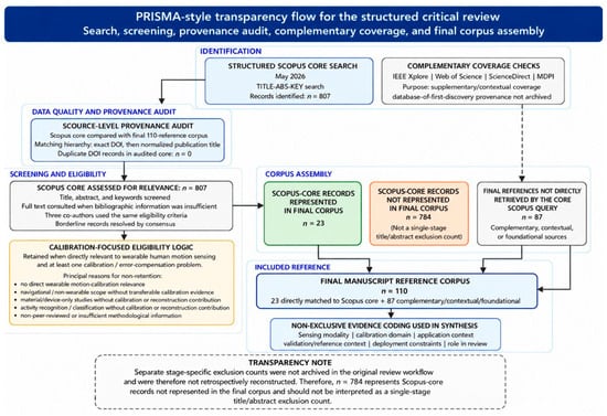
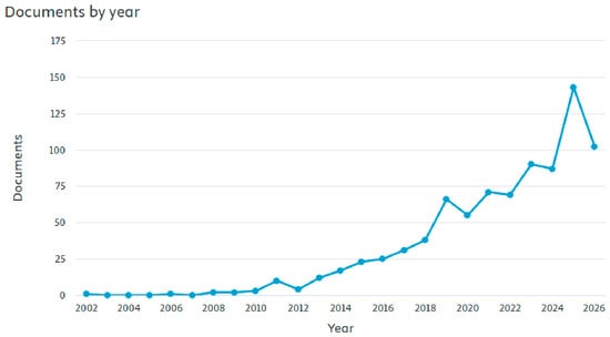
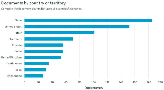
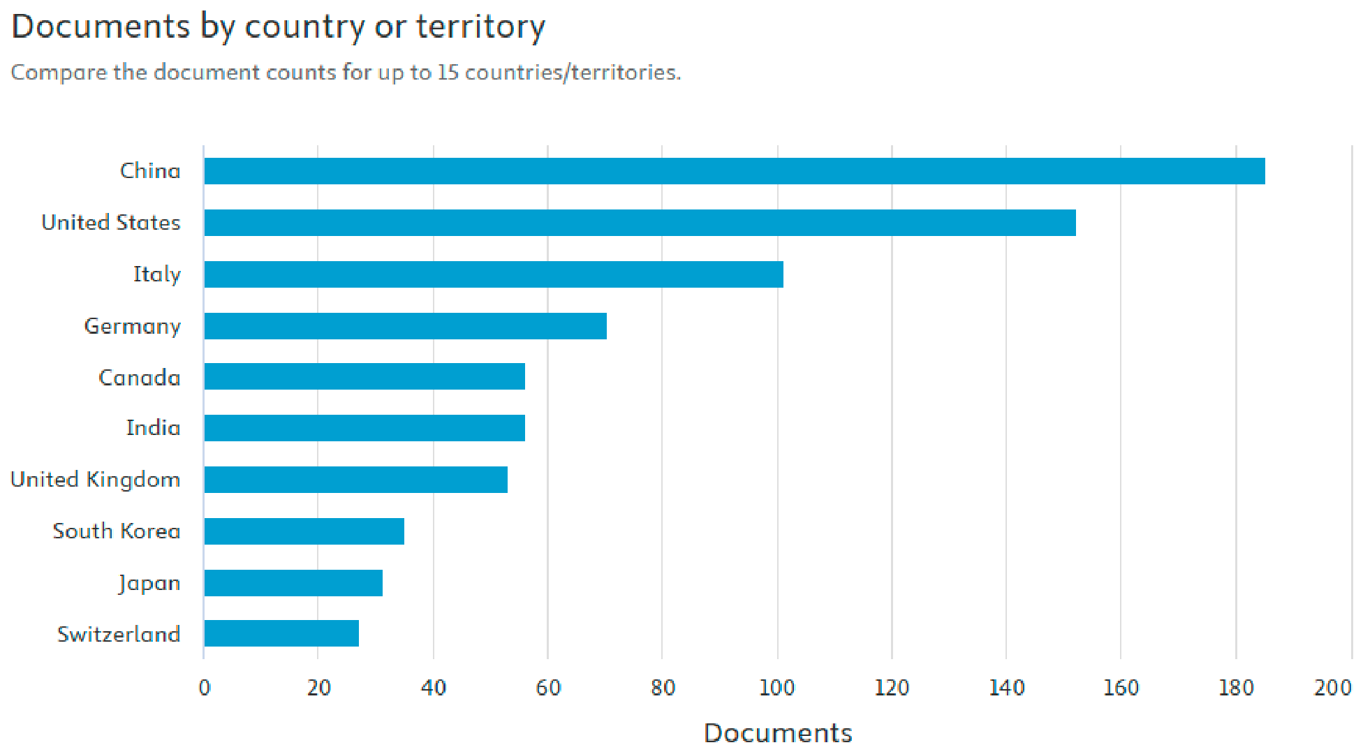
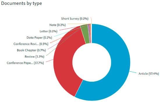
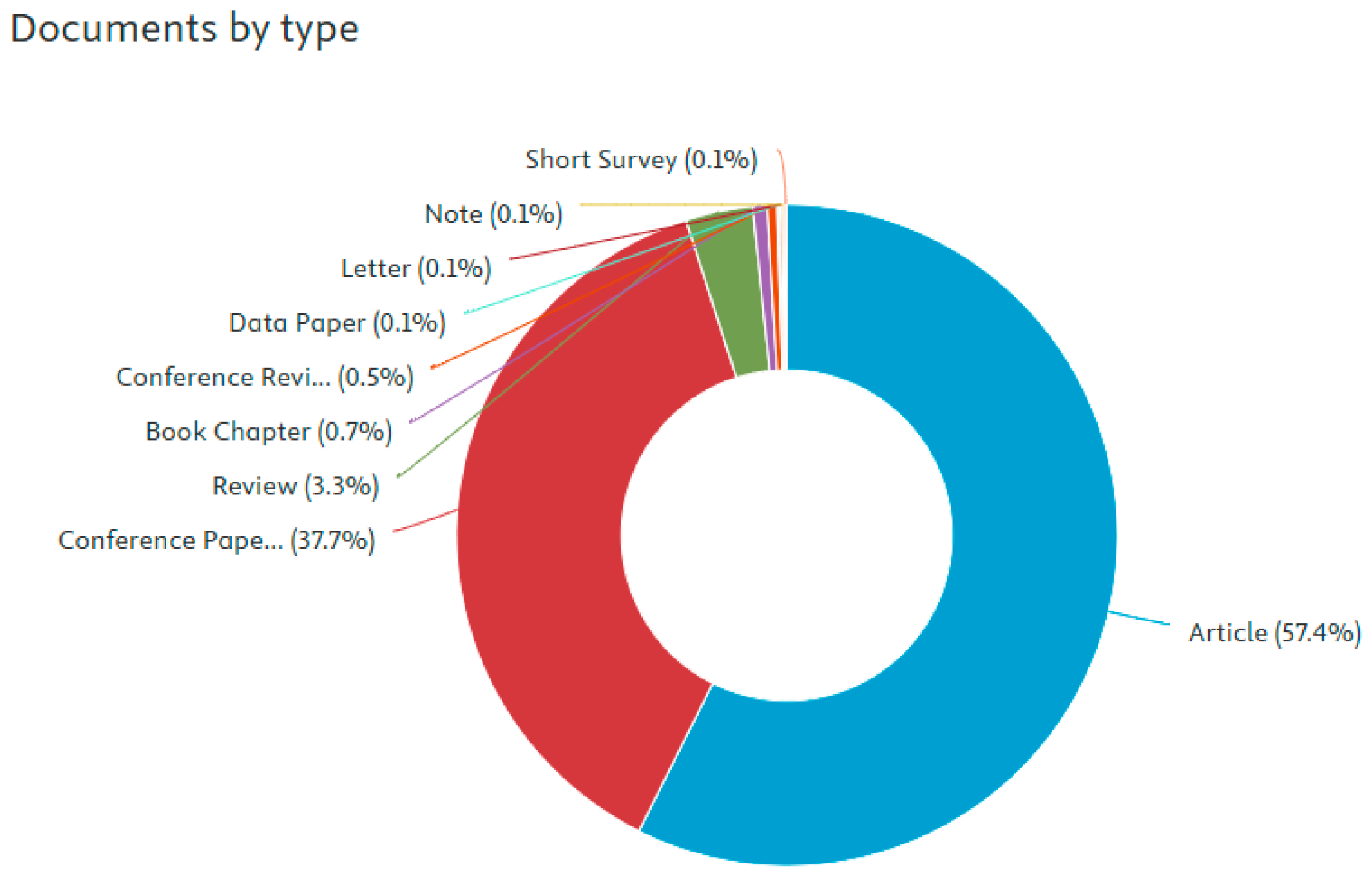
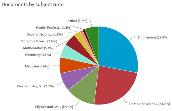
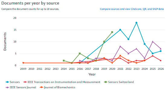
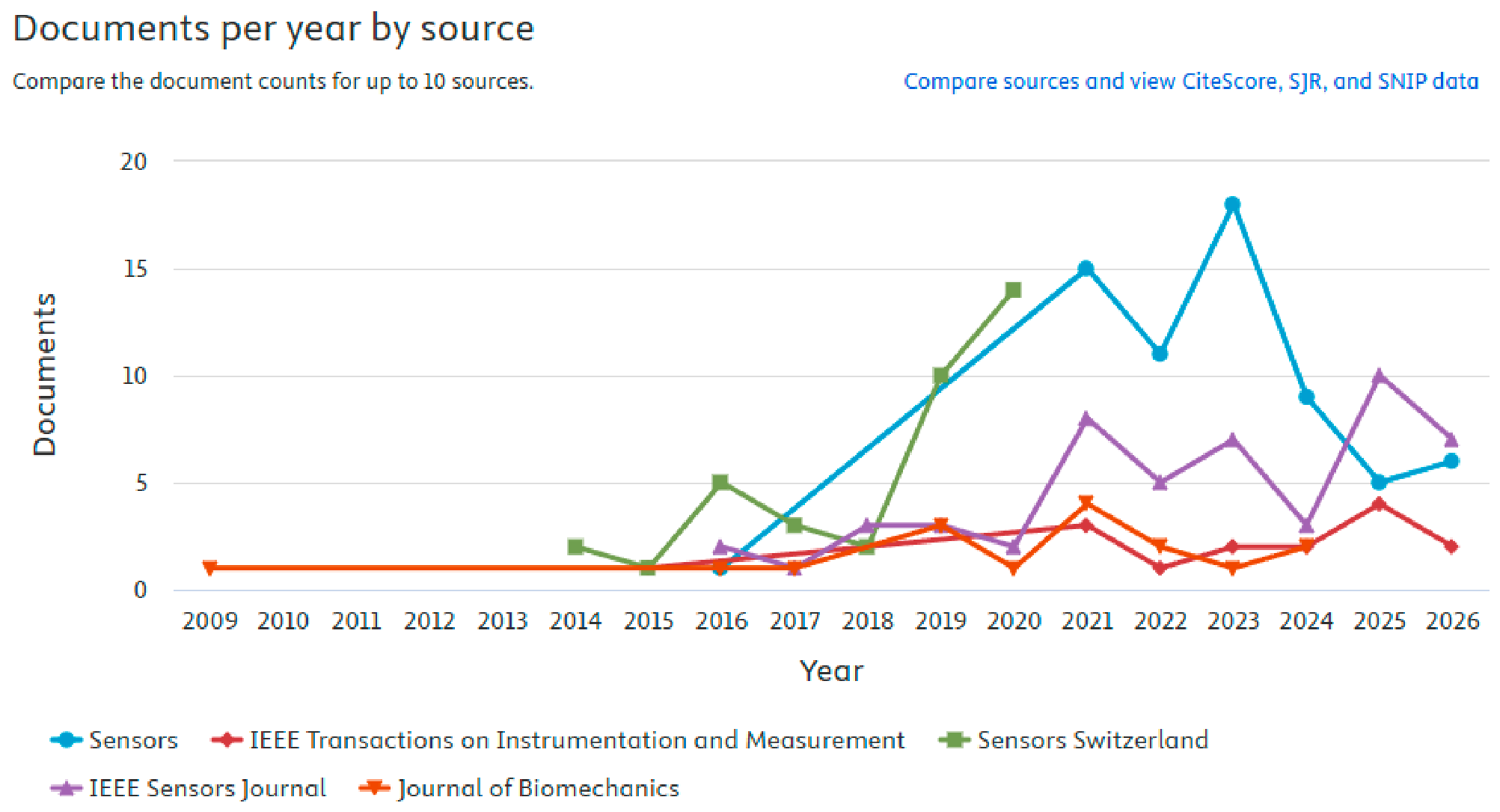
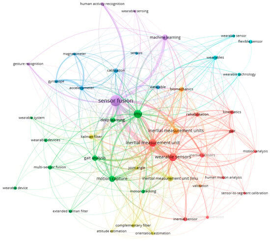
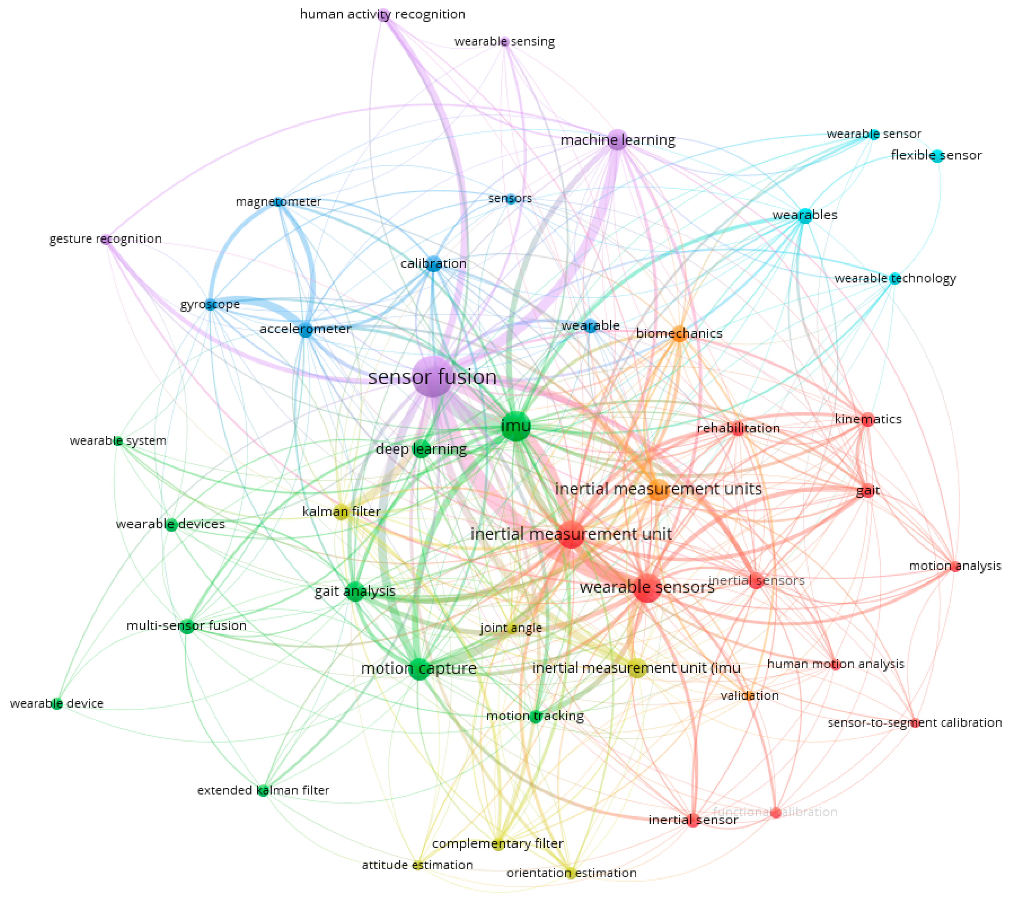
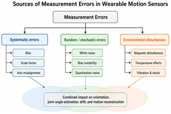
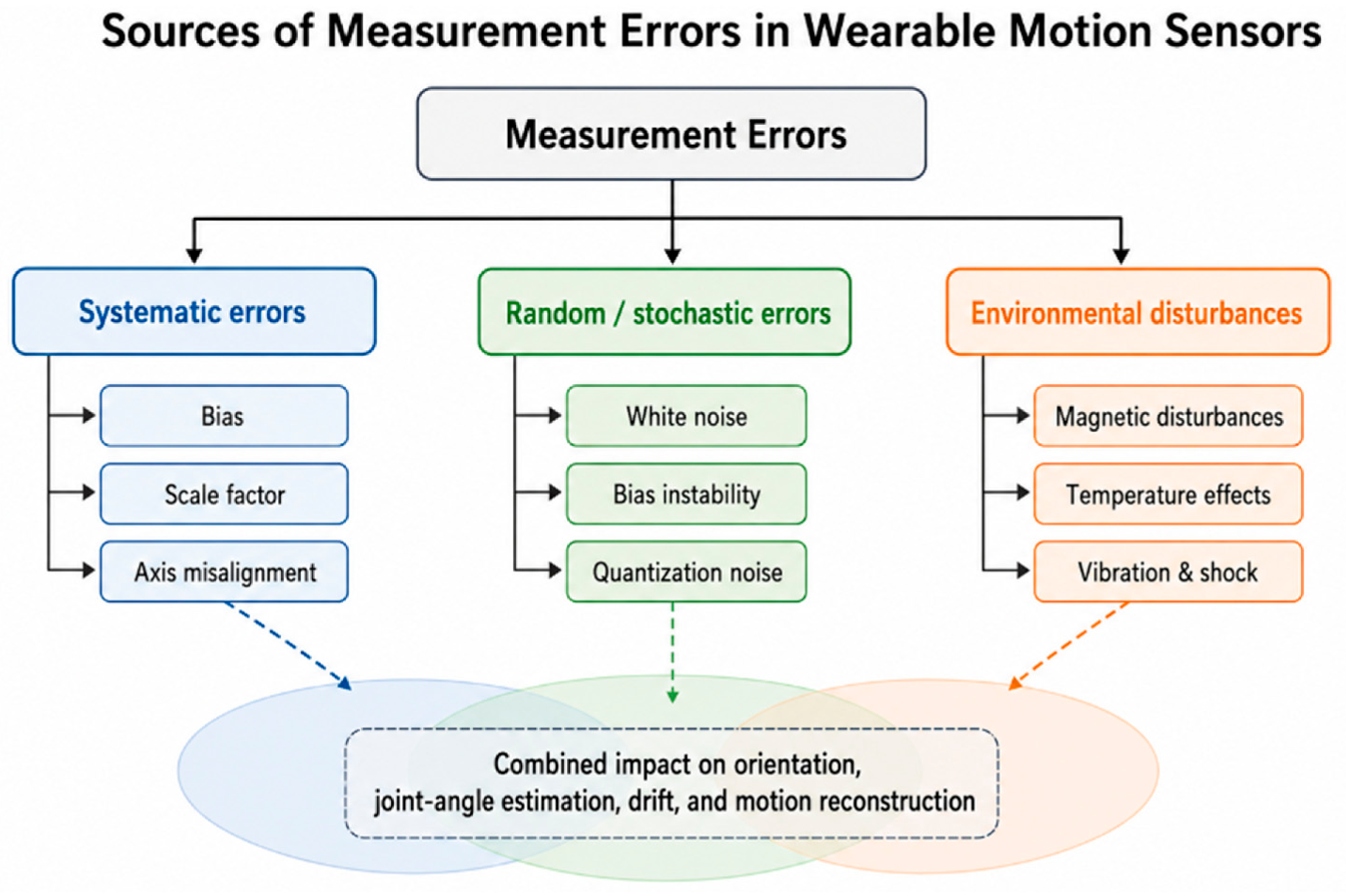
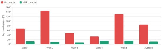
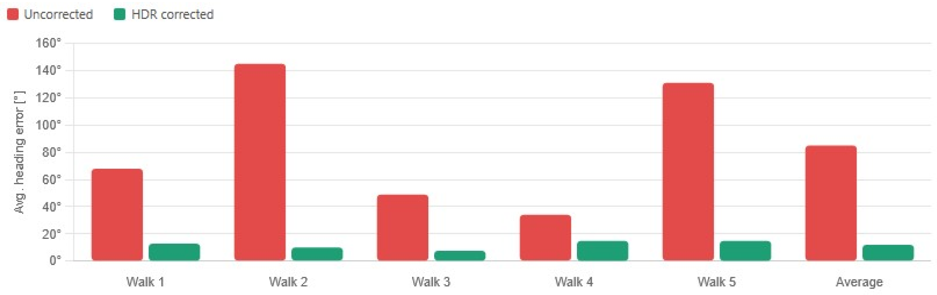
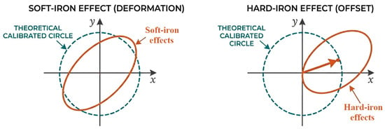
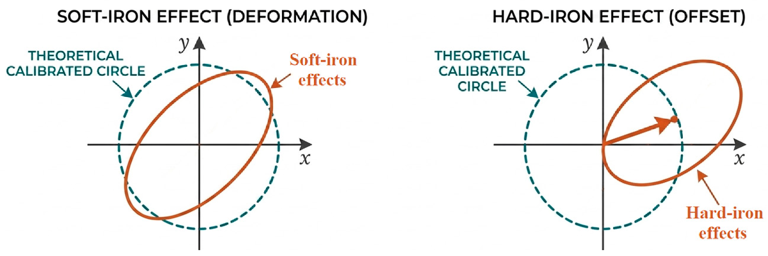
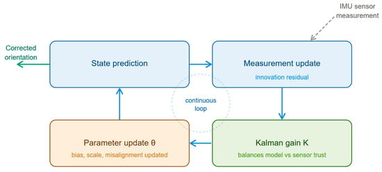
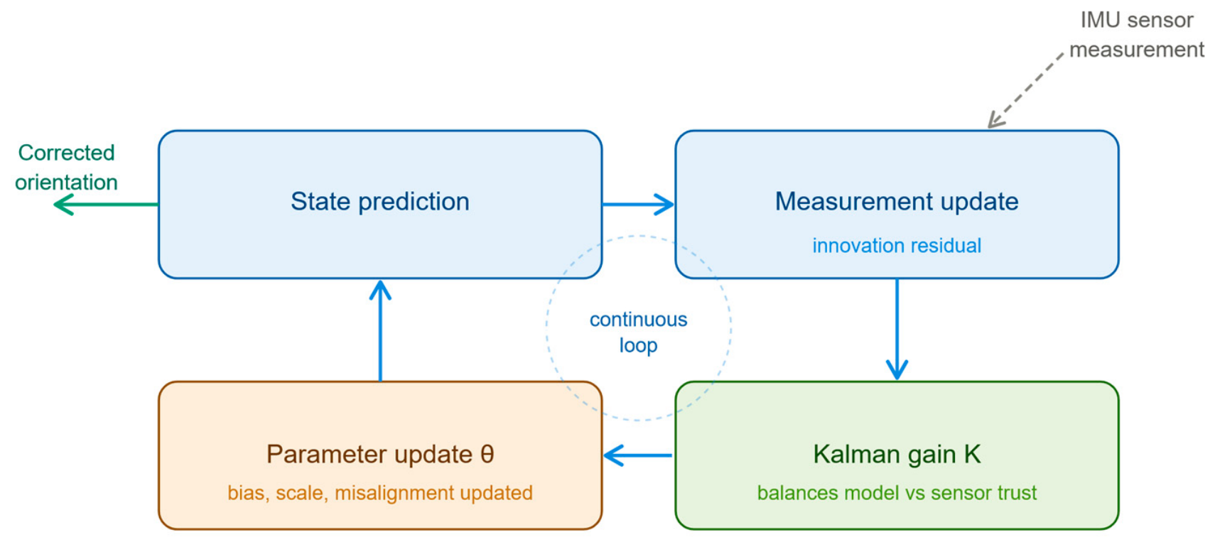
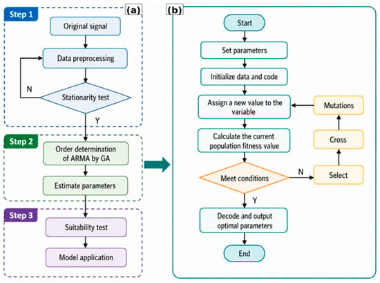
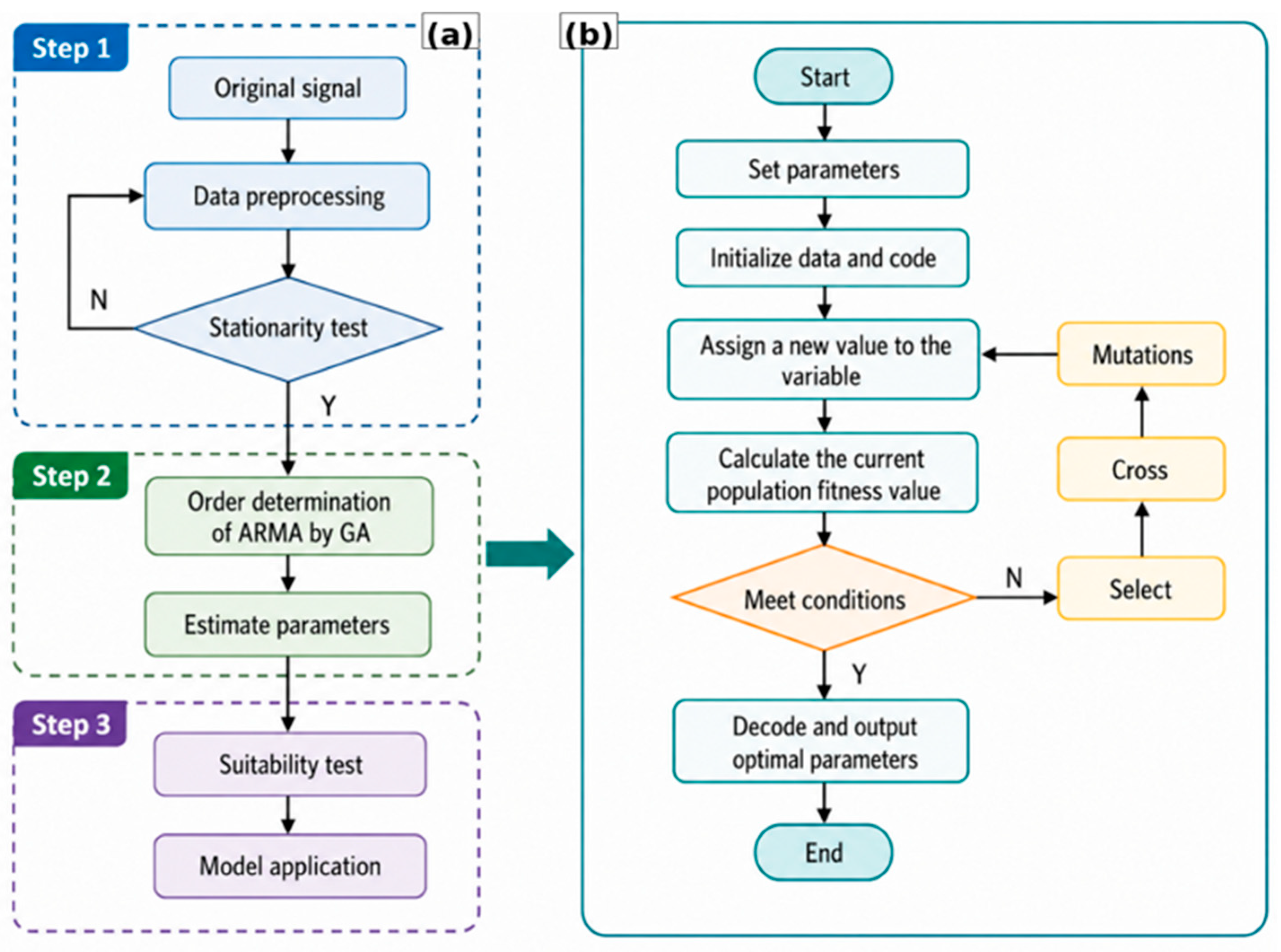
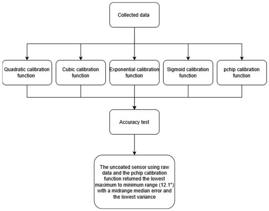
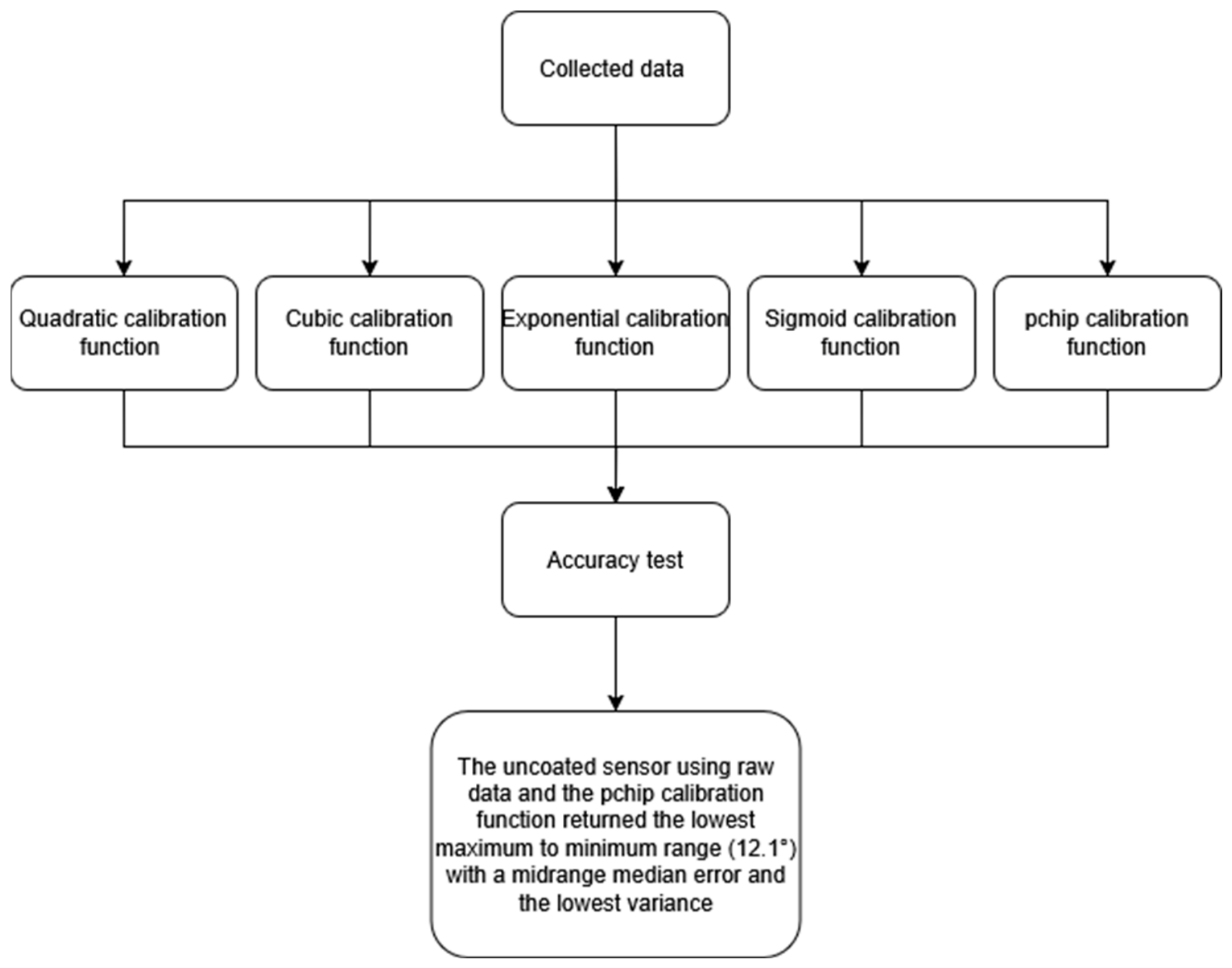
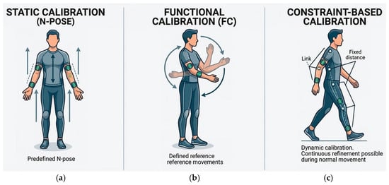
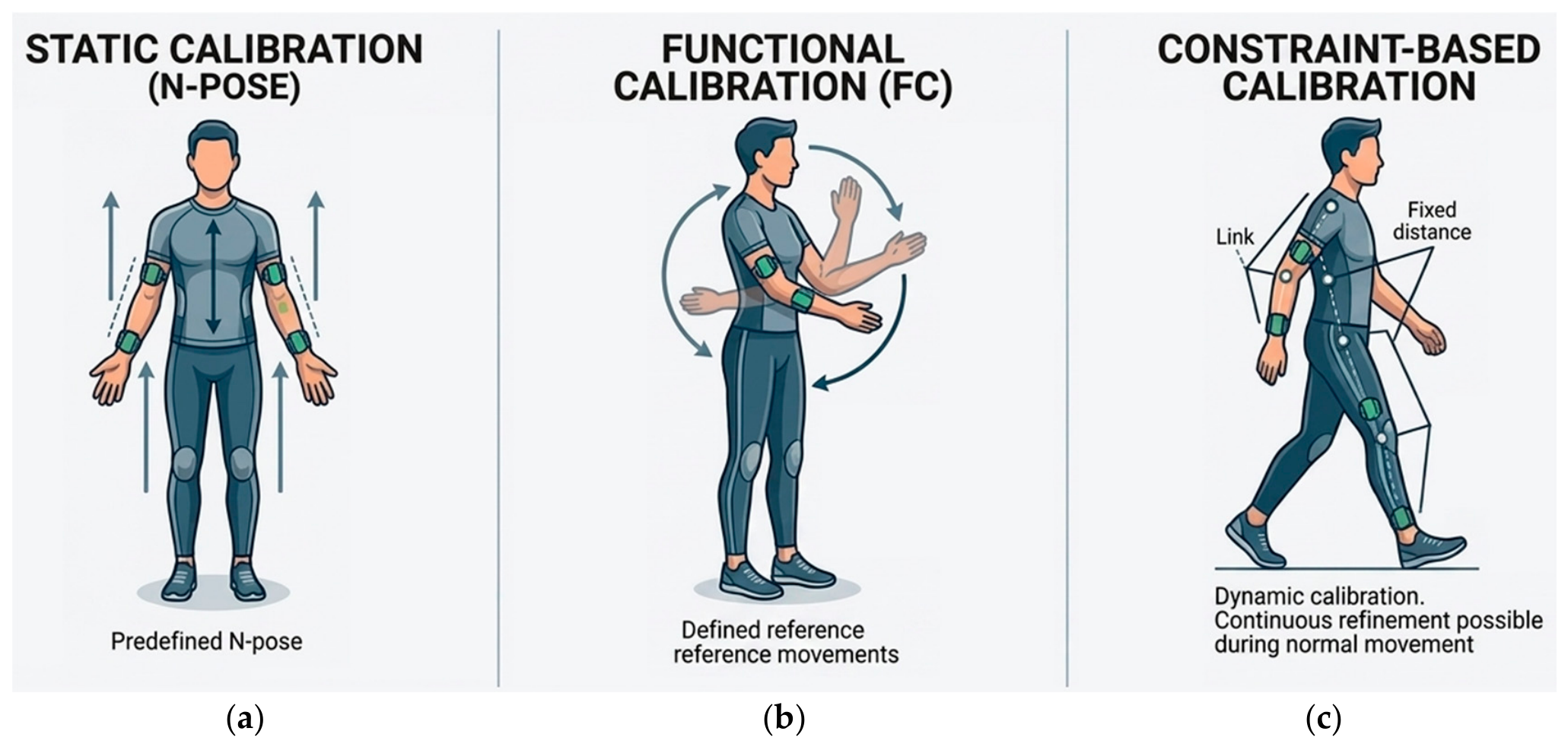
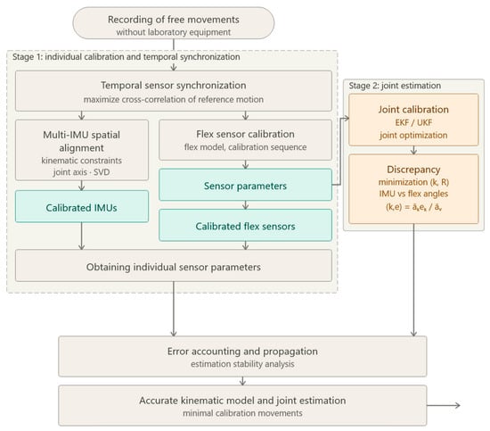
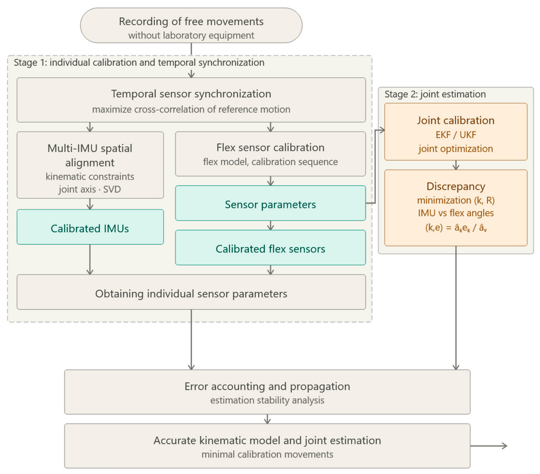
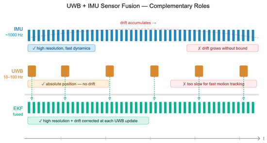
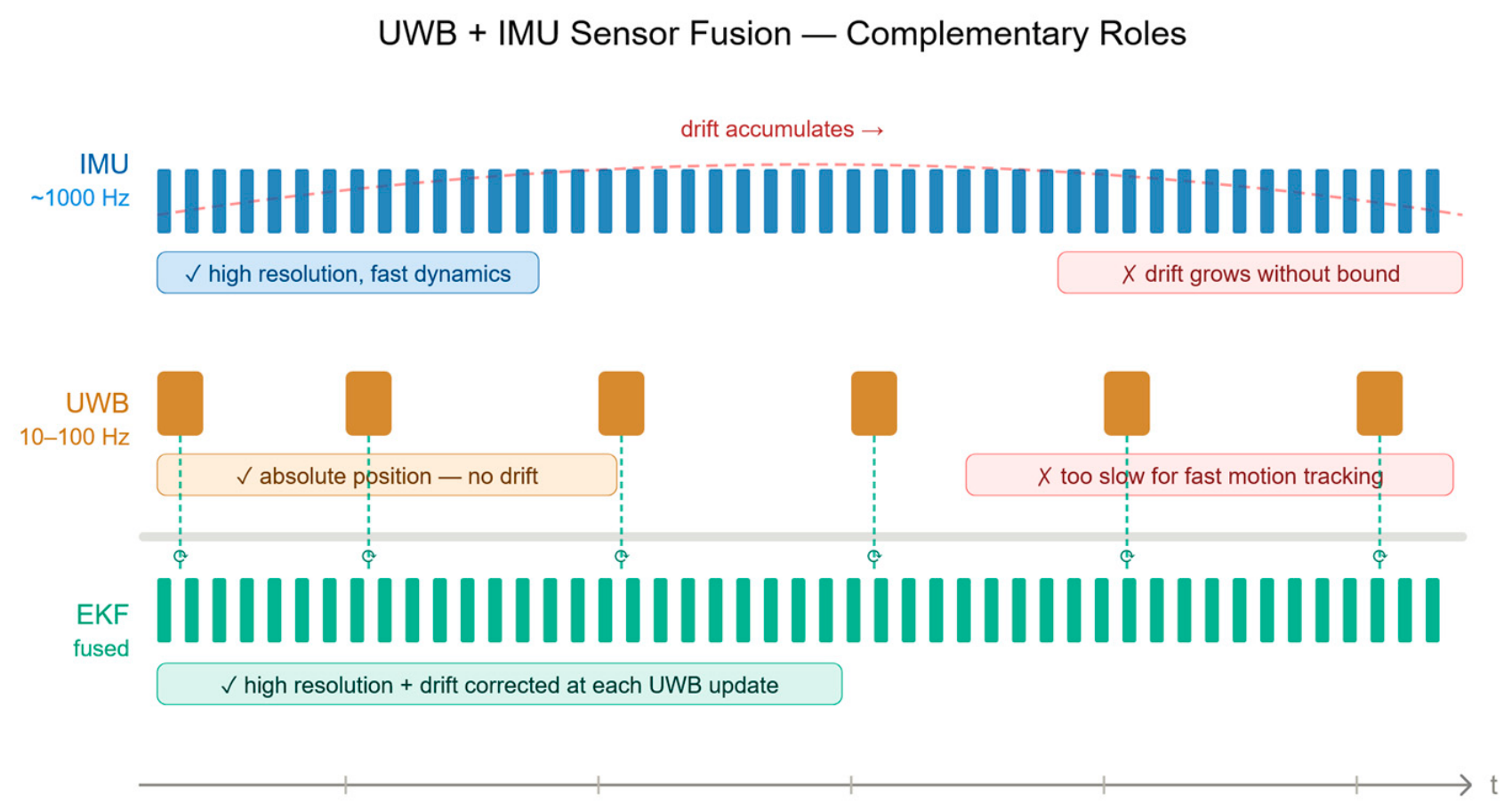

Disclaimer/Publisher’s Note: The statements, opinions and data contained in all publications are solely those of the individual author(s) and contributor(s) and not of MDPI and/or the editor(s). MDPI and/or the editor(s) disclaim responsibility for any injury to people or property resulting from any ideas, methods, instructions or products referred to in the content. |
© 2026 by the authors. Licensee MDPI, Basel, Switzerland. This article is an open access article distributed under the terms and conditions of the Creative Commons Attribution (CC BY) license.