


Abstract
This work proposes a comparative framework for malware classification that evaluates the synergy between traditional feature engineering and modern deep learning architectures. Our methodology follows two primary paths: first, we integrate opcode n-grams with word-embedding techniques (Word2Vec, Doc2Vec, and FastText) to capture local execution patterns in dense vector spaces. Second, we evaluate end-to-end representations using transformer-based models (BERT and ViT) and a raw opcode-based 1D Convolutional Neural Network (1D-CNN) to determine if effective features can be learned without explicit n-gram engineering. Both pathways are rigorously tested across a suite of classifiers, including Support Vector Machine (SVM), Random Forest (RF), k-Nearest Neighbor (k-NN), and CNNs. Experimental results for multi-class classification demonstrate that while transformer-based models offer high automated feature extraction capabilities, the combination of opcode n-grams with word embeddings remains a highly effective and interpretable approach for detecting real-world malware.
1. Introduction
In this digitally connected world, malware poses a serious and evolving threat to every computer system, as well as to the secure storage of data. Hackers design sophisticated software that appears harmless to gain access, cause disruption, and steal resources and sensitive information from computer systems [1]. The process of classifying such malicious software into distinct categories or families is known as malware classification. As malware continues to grow in complexity and diversity, effective techniques for its detection and classification have become increasingly important. Grouping malware into families helps us better understand the behavior and traits of each group. This understanding can aid in building threat detection and intelligence systems, conducting effective incident management, monitoring alerts, and developing defense strategies. For example, viruses, worms, and trojans are different malware categories. A virus attaches itself to a program or application, and when it runs, the virus activates and spreads further. A worm replicates itself and spreads over a network by exploiting security flaws. A trojan, on the other hand, appears to be a harmless program and uses social engineering to deceive users [2]. In addition to these categories, each malware family shares common attack patterns. For instance, Zbot operates on the Windows operating system and attempts to extract banking and credit card information [3].
Initially, malware was primarily detected using signature-based methods. These techniques rely on the unique signatures of objects, matching them to the signatures of known malware. If a match is found, it is added to the malware database [2]. However, due to the evolving nature of malware, newer methods for its detection have been introduced. The use of machine learning and artificial intelligence has shown promising results. This paper employs a combination of techniques to classify malware into families. We explore the integration of opcode n-grams and word-embedding techniques to classify malware. When malware executable files are disassembled, we can extract assembly-level instructions. These instructions consist of opcodes, which are acronyms that direct the CPU to perform specific operations. These opcodes are specific to a microprocessor’s architecture. Treating opcodes as words allows embedding techniques to capture sequential relationships between instructions, enabling the model to learn execution patterns characteristic of specific malware families.
In this work, we create n-grams from opcode sequences, ranging from bigrams to heptagrams. These opcode n-grams provide insights into local patterns exhibited by malware families. Using opcode n-grams as the foundation, we then generate word embeddings to transform opcode n-grams into dense vectors. In this way, we map discrete opcode n-grams into continuous numerical vectors, capturing context and semantics, which serve as feature vectors for our classification models. The word-embedding techniques explored include Word2Vec, Doc2Vec, and FastText. We employ a diverse set of classifiers such as Support Vector Machines (SVMs), Random Forest (RF), k-Nearest Neighbors (KNNs), and Convolutional Neural Networks (CNNs). Since each classifier has unique strengths, we conduct a comparative analysis of their performance across various embedding techniques. All experiments are carried out on a set of 10 malware families. Figure 1 summarizes the overall experimental framework. Starting from the malware binary dataset, opcodes are first extracted from each sample. From this common opcode representation, three parallel pathways are explored: (1) opcodes are grouped into n-grams and converted into embedded vectors using Word2Vec, Doc2Vec, and FastText; (2) the same opcode sequences are passed to transformer-based models, BERT and ViT, which learn representations directly; and (3) raw opcode sequences are fed to a 1D-CNN without any explicit feature engineering. The outputs of all three pathways are ultimately passed to the same classification framework (SVM, RF, k-NN, and CNN), allowing a direct comparison between explicit n-gram/embedding features and end-to-end learned representations.
Figure 1.
Layout of the experiments.
The remainder of this paper is organized as follows. Section 2 presents a detailed review of existing malware classification techniques and related literature. Section 3 explains the concepts and terminologies utilized in this work. In Section 4, we examine the dataset and briefly introduce the models implemented. In Section 5, we describe the experiments carried out, demonstrating that the proposed techniques are robust and effective in the classification of malware. Finally, Section 6 summarizes the paper’s findings and outlines potential future improvements.
2. Related Work
As malware classification has gained importance over the years, many different techniques have been researched. Broadly, this is achieved using static or dynamic analysis or even a combination of both [4]. Static analysis focuses on the source program or binary-level representation to understand the control flows and possible malicious patterns. There is no need to execute the program. In contrast, dynamic analysis focuses on executing the program in a virtual or controlled environment. During execution, various activities, such as network traffic, API calls, and other system activities, are monitored. The advantage of static analysis is that it is less resource-intensive, fast, and efficient. In the past, signature-based detection techniques have been used to identify risks. However, the shortcoming of this approach is that it is only useful for detecting known malware.
The authors of [5] extract opcodes from Portable Executable (PE) files and use TF-IDF weighting for n-grams by selecting the top 1000 opcode n-grams. They then use XGBoost, SVM, and DNN classifiers, achieving 96% precision and recall for XGBoost. Additionally, the authors of [6] create features from n-gram sequences of API calls and opcodes using TF-IDF for feature scaling. This framework achieved a high F1-score of 99%. In [7], the authors use n-grams of byte codes and sort them in descending order based on the information gain from byte codes. They use the top N n-grams as feature vectors and calculate attribute similarity by averaging feature vectors from malware and benign data separately. They conclude that 3-gram byte opcodes were the most efficient. In [8], the authors use byte unigrams with hex n-grams to obtain more information from the executable file. Models such as Random Forest and LightGBM were used, and the average accuracy was 99%. Along similar lines, the authors in [9] use the frequency of opcode sequences. The relevance of each opcode is determined by its occurrence in both malware and benign executable files. Classifiers such as SVM, Decision Trees, and Bayesian Networks were used, with SVM achieving the best result of 95.9%. These research approaches demonstrate that extracting n-grams from opcode sequences is a promising feature for malware classification.
Many studies have also used word-embedding techniques from natural language processing to represent features as multi-dimensional vectors. In [10], the authors reduce the length of opcode sequences by applying a Random Walk approach with edge and node selection to create a low-dimensional vector space. They discuss that this approach, along with Skip-Gram embedding, overcomes limitations caused by obfuscation techniques. Another study focuses on transformer architectures such as BERT, DistilBERT, ALBERT, and RoBERTa, as well as ELMo, to create contextualized word embeddings from opcodes [11]. The authors also compare these embeddings to the context-free embeddings generated from Word2Vec and HMM2Vec. Their research concludes that the DistilBERT model with CNN achieved a maximum accuracy of 97.85%. Another study takes a similar approach by focusing on opcode sequences for classification along with Word2Vec, HMM2Vec, BERT, and ELMo embedding techniques [12]. The authors compare and analyze the effects of different embeddings on classifiers such as SVM, RF, CNN, and k-NN. In another relevant study, the authors use opcode sequences and API call names to improve malware classification [13]. They employ the FastText model, which creates lower-dimensional vectors compared to one-hot encoding. The FastText model reduced the dimensionality by 80% and achieved a high accuracy of 98.14% when used with a Bi-LSTM model. In another interesting study, the authors define the Op2Vec embedding technique based on the Skip-Gram Word2Vec model to detect Android malware [14]. They create a dataset based on the trained Op2Vec model for end-to-end detection.
In [15], the author focuses on how classification can derive more insightful features from the data compared to using raw features directly. This research employs Hidden Markov Models (HMMs), Principal Component Analysis (PCA), and the neural network-based technique Word2Vec to generate embeddings from opcodes. The authors of [16] use opcodes containing CALL instructions to reduce the number of opcodes. Then, the Word2Vec model using CBOW (Continuous Bag-of-Words) is applied to generate embeddings. A Convolutional Neural Network (CNN) is then used to capture the semantic relationships between opcodes [16]. The proposed solution achieved an accuracy of 98.18%. In [17], the authors propose a framework called Instruc2Vec. The opcodes are extracted by disassembling software and are converted into vectors using the Skip-Gram model of Word2Vec. These vectors serve as inputs to deep learning algorithms such as CNN, LSTM, and Siamese networks, which can rapidly create and identify hidden features [17]. The experimental setup is then used to classify software as benign or malicious, demonstrating the potential to accelerate malware detection.
Recently, there has been a shift towards deep learning models for efficient malware classification. In one study, opcode sequences are extracted from binary files and passed to a Convolutional Recurrent Neural Network (CRNN) [18]. The model has two stages, that is, an Opcode-level Convolutional Autoencoder (OCAE) that is used to create compressed sequences from lengthy opcode sequences, and a Dynamic Recurrent Neural Network (DRNN) that is used as the classifier to detect malware. This experimental setup achieves an accuracy of 96%. Another study proposes a two-stage LSTM model to analyze opcode sequences [19]. This model includes two LSTM layers and a mean-pooling layer to extract feature representations of opcode sequences. The first layer processes opcode-embedded vectors, while the second layer generates hidden vectors representing different timesteps. The mean-pooling layer then averages them. The focus is to use LSTM to understand patterns in opcode sequences and reduce manual effort. An interesting study combines static and dynamic analysis to detect malware. The authors use opcode bi-grams and API call frequencies to capture the semantics and behaviors of malware [20]. The proposed solution implements two neural networks, CNN for opcode bi-grams and a Back-Propagation Neural Network (BPNN) for API features. These features are merged before classification, and this approach achieves around 90% accuracy for malware families.
The research suggests that opcodes and word embeddings are useful features for malware detection and classification. This forms the basis of our work, in which we experiment with different opcode n-gram ranges and word-embedding techniques to efficiently classify malware.
While the studies reviewed above establish that the opcode n-gram plus word-embedding paradigm is effective, each of them typically evaluates one embedding technique (most often only Word2Vec) paired with a small, fixed set of classifiers, on its own dataset. What is missing from the literature is a controlled study that varies the n-gram range, the embedding technique, and the classifier independently, under the same dataset and evaluation protocol, so that the effect of each choice can be isolated. Our work addresses this gap in four ways. First, we systematically sweep opcode n-gram sizes from 2 to 7, whereas most prior studies fix a single n-gram size a priori. Second, we compare three embedding families, Word2Vec, Doc2Vec, and FastText, each with both of their standard model variants (CBOW/Skip-Gram and PV-DM/PV-DBOW), rather than a single embedding choice. Third, we pair every embedding technique with the same four classifiers (SVM, RF, k-NN, CNN) using an extensive hyperparameter search (1116 combinations in total), enabling a like-for-like comparison across embeddings rather than across studies with different setups. Fourth, we extend the comparison beyond n-gram-based features to transformer-based representations (BERT, ViT) and a raw opcode 1D-CNN evaluated under the identical dataset and protocol, directly testing whether automated feature learning can match explicit opcode n-gram engineering. This combination of breadth and methodological control is what distinguishes our work from prior studies in this space.
3. Background
In this section, we discuss the methods, techniques, tools, and algorithms used in this research. The first part covers malware analysis, opcodes, and n-grams, including a discussion on malware families. We explain the importance of opcode n-grams and how different values of n affect the results. Following this, we briefly discuss statistical measures such as Term Frequency-Inverse Document Frequency (TF-IDF), and we explain the workings of various word-embedding techniques used in this research, including Word2Vec, Doc2Vec, and FastText. We then discuss the machine learning algorithms that we employed, such as Support Vector Machine (SVM), Random Forest (RF), k-Nearest Neighbor (KNN), and Convolutional Neural Network (CNN).
3.1. Malware Analysis
Malware is a piece of code or software created to damage systems or steal important data for financial gain or disruption [1]. Most of the time, such software appears benign and resembles legitimate software to users. Hence, there is an ever-increasing need to detect and classify malware. To better understand different types of malware, they are grouped into families. Collections of malware that share similar traits, behaviors, or origins are categorized into the same family. Malware belonging to the same family usually attacks in a similar manner and shares common vulnerabilities. These families also provide insights into how malware has evolved over the years [2]. In this research, we experiment with 10 malware families and perform multi-class classification. The details are covered in Section 4.
In static malware analysis, malware files are analyzed without execution. Opcodes are used to understand the execution flow in malware code. In machine language, an opcode is the initial byte of an instruction that tells the hardware what action to perform. Each processor type has a specific set of opcodes [21]. Opcodes can be represented in three formats:
- Byte grams: A sequence of raw byte values.
- Hex opcodes: Represented in hexadecimal format for better readability through debuggers or disassemblers.
- Text opcodes: Mnemonic representations such as “ADD,” “MOV,” and “SUB.”
Our experiments involve text opcodes. A single opcode considered in isolation carries little discriminative information, since the same instruction (e.g., MOV or PUSH) appears across almost all executables, benign and malicious alike. What tends to distinguish malware families is not individual opcodes but the sequence in which they occur, since this sequence reflects the underlying logic of the code. This motivates the use of n-grams, which group consecutive opcodes together so that short, recurring execution patterns can be captured and used as discriminative features. An n-gram is a continuous sequence of n elements from any text. Analogous to text data, we can extract n opcodes from malware files to create opcode n-grams. These n-grams can help identify characteristic patterns that indicate malicious behavior. In fact, different malware families exhibit distinct n-gram patterns, which can aid in classification. For example, malware that performs runtime unpacking or self-decryption often repeatedly executes a short loop such as XOR, INC, CMP, JNZ, which decrypts a block of code one byte at a time before it is executed; captured as a 4-gram, this exact sequence tends to recur many times within a single file and appears consistently across samples belonging to the same family, making it a strong discriminative signal even though none of the four opcodes is unusual on its own. Similarly, a sequence such as PUSH, PUSH, CALL commonly marks the point where arguments are set up immediately before an API call, and the specific opcodes surrounding this pattern tend to differ systematically between families that rely on different system services (e.g., network communication versus file encryption). This is the type of local, family-characteristic pattern that opcode n-grams are intended to capture. This approach could also help make systems more robust against obfuscation, since an attacker attempting to hide the true intent of their software may still leave the underlying local opcode patterns largely unchanged; however, we do not evaluate this robustness claim empirically in this study, as discussed further in Section 6. We experiment with n-gram sizes ranging from two to seven; we do not evaluate n = 1 (single opcodes in isolation) since, as noted above, individual opcodes carry very little discriminative information on their own and are shared across almost all executables, so a unigram representation would not be expected to capture the family-specific execution patterns that motivate this study. We start at n = 2 as the smallest window capable of capturing a local relationship between consecutive opcodes.
3.2. Statistical Measure
In this paper we use Term Frequency-Inverse Document Frequency (TF-IDF), which is a statistical measure primarily used in natural language processing to determine the importance of words in a document relative to the entire collection. It assigns a score to each word based on its frequency within a document, adjusted by its occurrence across the entire corpus. This adjustment accounts for the fact that some terms appear more frequently than others overall.
In this research, we begin by creating TF-IDF vectors for different n-gram ranges of opcode sequences. These vectors are then used as input for the SVM classifier, serving as our baseline model for classification. TF-IDF is particularly useful for identifying whether certain opcodes are indicative of malicious behavior.
3.3. Word-Embedding Techniques
While opcode n-grams are effective at capturing local, short-range patterns, they suffer from two well-known limitations. First, the number of possible n-grams grows exponentially with n, producing extremely sparse and high-dimensional TF-IDF vectors that discard information about how opcodes relate to one another. Second, TF-IDF treats every n-gram as an independent, unrelated token, so two opcode sequences that are functionally similar but not identical receive no credit for that similarity. Word-embedding techniques address both issues by learning dense, low-dimensional vector representations in which opcodes (or opcode sequences) that tend to occur in similar execution contexts are placed close together in the vector space. This provides a more compact and semantically meaningful representation than raw n-gram frequency counts, which is the primary motivation for exploring embedding-based features in this work.
Word-embedding techniques transform textual data into numerical vectors, capturing semantic relationships between words. These embeddings are widely used in Natural Language Processing (NLP) but can also be applied to malware analysis by treating opcodes as words. In this section, we discuss various word embedding methods such as Word2Vec, Doc2Vec, and FastText, which are used in this research.
3.3.1. Word2Vec
Word2Vec is a powerful technique for generating word embeddings, which are essentially vector representations of words. It was developed at Google, and the main idea is that similar words should have similar vector representations [22]. This is achieved using shallow neural networks, making it computationally efficient. Word2Vec generates dense vectors compared to one-hot encoding and captures semantic relationships. We can extend this technique from the field of natural language processing and apply it to opcodes. In the context of malware classification, we treat opcodes as words in a sentence. There are two models within Word2Vec, that is, Continuous Bag-of-Words (CBOW) and Skip-Gram (SG).
3.3.2. Continuous Bag-of-Words (CBOW)
CBOW predicts a word based on its context. Surrounding words within the window size form the context for the target word. For example, in the sentence “Malware classification with Word2Vec,” if the window size is 2 and the target word is “classification,” the context words are “Malware,” “with,” and “Word2Vec.” This model has three layers, that is, input, hidden, and output. The input layer receives the context words. The embeddings are then passed to the hidden layer, which averages them. These are finally passed to the output layer, a Softmax layer, which predicts the target word, yielding its probability distribution. CBOW typically performs better on larger datasets.
3.3.3. Skip-Gram
Skip-Gram is the inverse of CBOW. It predicts the surrounding context based on the target word. For example, in the sentence “Malware classification with Word2Vec,” for the target word “classification,” this model predicts context words like “Malware,” “with,” and “Word2Vec.” This model also has three layers. The first step obtains word embeddings for the target and context word pairs. The hidden layer computes the dot product of these embeddings. The output layer is a dense sigmoid layer. The output is compared with the real label, and the loss is determined using backpropagation [23]. It works well with smaller datasets.
3.3.4. Doc2Vec
Doc2Vec is an extension of Word2Vec. Its aim is to create vector representations of a document regardless of its length [24]. It overcomes the limitation of Word2Vec, which only creates individual word embeddings. Doc2Vec is useful for capturing the overall context and semantic meaning of the document. Its design is similar to Word2Vec, except that the authors added another vector known as the paragraph or document vector [25]. Like Word2Vec, Doc2Vec also has two models, PV-DM and PV-DBOW.
3.3.5. Distributed Memory Version of Paragraph Vector (PV-DM)
In this model, we have a document vector that is unique to every document. The prediction of the target word depends on both the context and the paragraph vector. This vector stores the paragraph’s context, which helps when the current data lacks previous context. The DM model is used when the order of words in the document is important.
3.3.6. Distributed Bag-of-Words Version of Paragraph Vector (PV-DBOW)
The DBOW model is similar to the Skip-Gram model in Word2Vec. Instead of using context word vectors, it uses a document vector to predict words randomly sampled from the document. DBOW is typically faster than the DM model and is used when word ordering is not crucial.
3.3.7. FastText
Word2Vec generates word representations by assigning vectors to each word. However, this method has limitations in the context of languages with a large number of rare words or extensive vocabularies [26]. FastText, developed at Facebook, was designed to overcome this limitation. It represents each word as a collection of character n-grams [26]. This enables the model to understand similar words based on internal characters, capturing the meaning of sub-words. Once the model trains on character n-grams, the resultant word embedding is the sum of all its n-gram vectors. FastText also has two models identical to Word2Vec: CBOW and Skip-Gram. A key advantage of FastText is that it can create embeddings for words it has never seen before. However, it requires more computational time since the model size increases due to sub-words. Another limitation is that it cannot capture the entire context, similar to Word2Vec.
3.4. Machine Learning Classifiers
After extracting opcodes, we experiment with different n-gram ranges. Using the word-embedding techniques, we obtain dense vectors. The next step is to train various machine learning algorithms to classify malware. Several studies have shown that classifiers such as SVM, RF, k-NN, and CNN have proven to be effective [5,8,9,12]. Our experimental results confirm that these classifiers are effective for multi-class classification, and here we give a brief description.
3.4.1. Support Vector Machines
Support Vector Machines (SVM) are used for both classification and regression tasks and can handle both linear and nonlinear data. SVM operates by creating a hyperplane that separates data points from different classes. The distance between the hyperplane and the nearest data point is called the margin. Support vectors are the data points closest to the hyperplane. The hyperparameter C controls the trade-off between maximizing the margin and minimizing classification errors. A kernel function is used to map the input data to a higher-dimensional space. We experiment with different types of kernel functions, such as linear, polynomial, and radial basis function (RBF). Further information about SVM, its applications, trends, and challenges can be found in [27].
3.4.2. Random Forest
Random Forest, originally introduced by Breiman [28], is well-suited for handling complex datasets and can be used for both classification and regression tasks. Random Forest uses multiple decision trees to determine the final output. In a decision tree, each node represents a decision, each branch represents an outcome for a test, and the leaf node provides the class label for classification tasks. Random Forest employs sampling with replacement to create subsets of data, resulting in each decision tree receiving a different subset. At each decision node, the algorithm uses only a random subset of the training features, which helps the trees to remain independent and less prone to noise. The advantages of Random Forest include higher accuracy and less susceptibility to overfitting. However, since it uses a large number of decision trees, it can become computationally expensive.
3.4.3. k-Nearest Neighbors
First proposed by Cover and Hart [29], KNN operates on the principle that similar data points will be close to each other in the feature space. Given a value of k, the algorithm identifies the k nearest data points to a target point and makes predictions based on their class labels. KNN offers different distance metrics such as Manhattan, Euclidean, and Minkowski to calculate distances between data points. Selecting the value of k is critical; in fact, a small k may make the model sensitive to noise, while a large k might overlook local patterns. One advantage of KNN is that it does not require a training phase. However, its limitations include sensitivity to the value of k and the choice of distance metric.
3.4.4. Convolutional Neural Network
A CNN is a deep learning model initially designed for computer vision tasks, such as detecting objects and classifying images. However, its applications have expanded to include language processing. CNN models consist of several layers, with the core concept being convolution. Convolution involves applying a filter to small sections of the input data and sliding it over the rest of the input, allowing the model to detect local features. Another key component is the pooling layer, which reduces the dimensionality while retaining essential information. After a combination of convolutional and pooling layers, CNN models include fully connected layers. These layers are used to make final predictions, with each neuron in the previous layer connected to a neuron in the next layer, enabling the model to take full context into account. Activation functions such as ReLU introduce nonlinearity, and loss functions measure the error between actual and predicted values. More details on the functioning of CNNs can be found in [30].
3.4.5. Bidirectional Encoder Representations from Transformers
BERT is a transformer-based model, built by Google, that learns contextual representations of text by processing input bidirectionally, considering both left and right context simultaneously. It is pre-trained on large corpora using two objectives: masked language modeling, where random tokens are masked and the model learns to predict them, and next sentence prediction, where the model learns relationships between sentence pairs. This pre-training allows BERT to capture deep semantic relationships, and the model can subsequently be fine-tuned for downstream classification tasks. However, BERT has notable limitations, including high computational cost due to its large number of parameters, and a fixed input length constraint that may cause truncation of longer sequences.
3.4.6. Vision Transformer
Vision Transformer (ViT) adapts the transformer architecture to image classification by dividing an image into fixed-size patches and treating them as sequential tokens. Each patch is linearly embedded and fed into a standard transformer encoder, where self-attention mechanisms allow the model to learn global relationships across patches. Unlike convolutional neural networks, ViT does not rely on local feature extraction, instead capturing long-range dependencies across the entire image. However, ViT has notable limitations, including a heavy reliance on large amounts of training data to perform effectively, and significant computational cost during both training and inference due to the quadratic complexity of self-attention.
4. Experimental Setup
This section provides details on the experimental setup used in this study, including the dataset and data preprocessing steps.
4.1. Dataset
The dataset used in this research consists of malware samples downloaded from VirusShare [31], and the ground-truth family label for each sample is taken directly from the VirusShare metadata under which the sample was collected. The executable files are disassembled using the objdump utility, and the opcodes are extracted from the resulting disassembly output [32]. We focus on 10 different malware families. The description of each malware family is as follows:
- Winwebsec: This family uses social engineering tactics to trick users into paying money for fake software or security updates. It generates fake popups and security messages claiming that the system is under a security threat.
- Zbot: Also known as Zeus, Zbot is designed for financial gain. It steals sensitive information, particularly banking, financial, and login details. It can also record keystrokes to capture critical data.
- Vundo: Virtumonde or Vundo spreads via malicious email attachments, unsafe downloads, or outdated software. It displays advertisements through pop-ups and banners and can direct users to malicious sites. Vundo is also capable of stealing data and causing identity theft.
- VBInject: VBInject is a packaging malware used to conceal other viruses. It uses compression and encryption to obfuscate its content [33].
- OnlineGames: OnlineGames targets gaming users through compromised game downloads. It can collect sensitive information and steal account credentials for fraudulent purposes.
- ZeroAccess: ZeroAccess spreads through compromised downloads and hides within the system using rootkit techniques. It creates a botnet by spreading across many systems, which attackers can then use for Denial of Service attacks.
- Injector: This malware injects harmful code into legitimate software, often targeting process memory or dynamic link libraries. Detecting it is challenging, as it typically operates within legitimate programs.
- FakeRean: FakeRean deceives users into thinking it is legitimate antivirus software by generating fake warnings and alerts. This tricks users into paying for fake software.
- Renos: Renos downloads malicious software that displays alerts claiming that the system is compromised, scaring users into paying money to “clean” their system [34].
- Zegost: Zegost is a backdoor malware that infiltrates systems via shady website downloads. It is capable of executing files, transferring information, and downloading other files [35].
The dataset consists of disassembled malware executable files. Each file contains all the opcodes from the code section. There were some duplicate files, and the preprocessing step involved selecting unique files using an MD5 hash. After this, the opcodes from each file were concatenated to form an opcode sequence. Each malware family contains a different number of samples, as shown in Figure 2. We randomly selected 500 samples from each family, resulting in a total of 5000 malware samples for all subsequent experiments.
Figure 2.
Count of samples per malware family.
4.2. Preprocessing
To establish a baseline for our experiments, we first use opcode sequences without applying n-grams. We extract a set of unique opcodes from the entire opcode sequence. In total, we identify 1704 unique opcodes. As these opcodes are mnemonic, we need to convert them into numerical vectors. For each malware sample in our dataset, we create a vector of length 1704. This vector is constructed by computing the frequency of occurrence of each unique opcode in each malware sample.
Next, we calculate the percentage of each unique opcode within the vector by dividing its frequency by the total number of opcodes in each malware file. Thus, the vector for each sample consists of the percentage of frequency of occurrence of each opcode. These vectors are then used to train machine learning algorithms for classification.
The dataset is split into 80% training data and 20% test data, using stratification to ensure equal class distribution. Specifically, we apply Support Vector Machine (SVM), Random Forest (RF), k-Nearest Neighbor (kNN), and Convolutional Neural Network (CNN) classifiers. The confusion matrices for SVM, RF, k-NN, and CNN classifiers are shown in Figure 3, Figure 4, Figure 5 and Figure 6, respectively. Table 1 provides a comparison of accuracy for all classifiers.
Figure 3.
Confusion matrix for opcode frequency-SVM.
Figure 4.
Confusion matrix for opcode frequency-RF.
Figure 5.
Confusion matrix for opcode frequency-KNN.
Figure 6.
Confusion matrix for opcode frequency-CNN.
Table 1.
Classifier accuracy comparison using opcode frequency.
After obtaining the opcode sequences, we create n-gram opcodes, with values of n ranging from 2 to 7. The primary goal of creating n-grams is to capture local patterns that may distinguish different malware families. Since the opcode sequence for each sample can be quite long, breaking it down into n-grams makes it more manageable. Additionally, instead of comparing the entire sequence when detecting similarities between malware samples, we can compare n-gram opcodes to identify recurring patterns. There is a trade-off when choosing values for n. If n is too small, we obtain highly granular features but lose contextual information. If n is too large, the context is captured, but the model may become prone to overfitting. Moreover, as n increases, the computational cost grows significantly.
We use the TF-IDF vectorizer from the sklearn Python (version 3.10.12) package to convert the n-gram opcodes into vectors [36]. Term Frequency (TF) calculates how often a term (or n-gram) appears in a given text, while Inverse Document Frequency (IDF) assesses how rarely the same term appears across the entire dataset. The IDF score increases when a term is rare in the dataset. The TF-IDF score is the product of TF and IDF values, highlighting terms that are important but not too frequent. We apply TF-IDF for all n-values in the range 2 to 7. For each of these values, we run SVM classification to predict the malware family, establishing a second base model for comparison.
Our results show that when n = 3, we achieve the best performance, with an accuracy of 92% and an F1 score of 92%. For other values of n, the accuracy and F1 score range between 89% and 91%. When we increase n beyond 3, there is no further improvement in these metrics, suggesting that tri-grams serve as the optimal feature for classification. Table 2, Table 3 and Table 4 present classification reports for n-values of 2, 3, and 6, respectively. Table 5 summarizes the accuracy for all n-gram opcodes tested with TF-IDF and SVM.
Table 2.
Classification report for n-gram = 2.
Table 3.
Classification report for n-gram = 3.
Table 4.
Classification report for n-gram = 6.
Table 5.
Accuracy comparison for opcode n-gram.
4.3. Word Embeddings Setup
To avoid data leakage, the 80/20 stratified train–test split described in Section 4 is performed before any embedding model is trained. All three embedding techniques, Word2Vec, Doc2Vec, and FastText, are fit exclusively on the training partition of the data. The resulting trained embedding models are then used to transform both the training and test samples into feature vectors; the test set itself is never used to fit any embedding model or classifier and is only used for final evaluation.
Word2Vec and FastText produce a single vector for each opcode tri-gram rather than for the malware file as a whole. To obtain one feature vector per malware sample, we average the vectors of all opcode tri-grams contained in that sample’s opcode sequence, producing a single fixed-length vector per file. Doc2Vec, by contrast, is trained directly at the document level, so each malware file is assigned its own document vector without requiring an additional averaging step. We repeated the embedding training and classification pipeline for n-gram sizes 2 through 7, consistent with the TF-IDF baseline; across all three embedding techniques, n = 3 again produced the best classification performance, mirroring the trend observed with TF-IDF and SVM. For this reason, the remainder of the embedding experiments reported in this section use opcode tri-grams (n = 3), which we adopt as the standard n-gram size for the rest of this work.
The first embedding technique applied to opcode tri-grams is Word2Vec. As previously discussed, we test both the Continuous Bag-of-Words (CBOW) and Skip-Gram models. The hyperparameters evaluated in this experiment are presented in Table 6. In total, we tested 24 combinations of Word2Vec embeddings. These embeddings are then passed to the SVM classifier to determine which combination of hyperparameters yields the best performance.
Table 6.
Hyperparameters tested for Word2Vec. A total of 24 parameter combinations were tested (2 models × 3 vector sizes × 4 window sizes).
One of the critical hyperparameters is the vector size, which defines the dimensionality of each word in the vector space. A smaller vector size might fail to capture detailed semantic information, while a larger vector size can model complex relationships but at the cost of higher computational resources and larger datasets. The window size, which controls the context considered around each word, is another crucial hyperparameter. Smaller window sizes capture local syntactic information, while larger windows capture broader semantic relationships. We use the Word2Vec model from the Gensim (version 4.4.0) Python library [37], and the tested hyperparameter combinations are detailed in Table 6.
From this experiment, we observe that the CBOW model outperforms the Skip-Gram model. The CBOW model achieves an accuracy of 86% with a vector size of 100 and a window size of 5, while the Skip-Gram model achieves an accuracy of 82% with the same vector size and window size. Figure 7 shows the accuracy details for all combinations of vector size and window size for both CBOW and Skip-Gram models.
Figure 7.
Word2Vec: CBOW v/s Skip-Gram comparison for hyperparameters.
Since Doc2Vec is an extension of Word2Vec, it shares similar hyperparameters. We experiment with both models of Doc2Vec, that is, Paragraph Vector Distributed Memory (PV-DM) and Paragraph Vector Distributed Bag-of-Words (PV-DBOW). For consistency and to limit the size of an already large hyperparameter search (1116 classifier combinations across embedding techniques), we reuse the hyperparameters found optimal in the Word2Vec experiments, with vector size = 100 and window size = 5, rather than performing an independent sweep for Doc2Vec; we discuss this design choice further as a limitation in Section 6. We use the Doc2Vec model from the Gensim library in Python [38].
We also experiment with both models of FastText, Continuous Bag-of-Words (CBOW) and Skip-Gram. As with Doc2Vec, for practical reasons we reuse the best hyperparameters obtained in the Word2Vec experiments (vector size = 100, window size = 5) rather than independently tuning FastText, a design choice we revisit in Section 6. FastText allows us to work with subword information, making it useful for capturing rare words. We use the FastText model from the Gensim library in Python [39].
4.4. Classifiers
In our experiments, we utilize four classifiers, that is, Support Vector Machine (SVM), Random Forest (RF), k-Nearest Neighbor (k-NN), and Convolutional Neural Network (CNN). The input data is split into 80% training and 20% testing data. We apply stratification during the split to ensure equal representation of samples from each class in the test set.
Hyperparameters play a key role in determining model behavior and performance. Therefore, tuning hyperparameters is crucial to achieving optimal results. To explore various parameter combinations, we employ GridSearch, a technique that exhaustively searches through all potential hyperparameter combinations. In addition, we combine GridSearch with cross-validation to further enhance model evaluation. In our experiments, we use k-fold cross-validation with k = 5, meaning the model is trained five times, each time using one subset for validation and the other four subsets for training.
The GridSearch and cross-validation are applied only to the training data, ensuring that the test data is kept unseen by any of the classifiers. This approach helps prevent overfitting or underfitting of the models. Cross-validation ensures that the models generalize well and do not perform poorly on unseen data. For SVM, we evaluate 60 hyperparameter combinations. For RF, we test 864 combinations, and for k-NN, we explore 144 combinations. In the case of CNN, we test 48 hyperparameter combinations. Overall, we evaluate a total of 1116 hyperparameter combinations across all embedding techniques, as summarized in Table 7. The results for each classifier, for each embedding type, are presented in the following sections.
Table 7.
Hyperparameters tested for classifiers.
5. Results
In this section, we present the results of various classification techniques, comparing their effectiveness in detecting and classifying different families of malware. The experiments are performed using a balanced dataset of malware samples, and all experiments are executed in a high-performance computing environment.
5.1. Word2Vec CBOW Model
The best hyperparameters for SVM with Word2Vec were C = 100, gamma = 0.1 and kernel = rbf. The overall accuracy was 93% and F-1 score was 93%. Classes 0 and 9, i.e., Zeroaccess and Zbot malware families, were perfectly predicted, as shown in Figure 8.
Figure 8.
Confusion matrix for Word2Vec CBOW-SVM.
The best hyperparameters for RF with Word2Vec were max_depth = 30, max_features = log2, min_samples_leaf = 1, min_samples_split = 2, n_estimators = 400. The overall accuracy was 92.7% and F-1 score was 92.6%. RF also has very close performance metrics to that of SVM. Figure 9 shows the confusion matrix.
Figure 9.
Confusion matrix for Word2Vec CBOW-RF.
The best hyperparameters for kNN with Word2Vec were algorithm = auto, metric = euclidean, n_neighbors = 3, weights = distance. The overall accuracy was 91.9% and F-1 score was 91.8%. Figure 10 shows the confusion matrix.
Figure 10.
Confusion matrix for Word2Vec CBOW-KNN.
The best hyperparameters for CNN with Word2Vec were batch_size = 32, dense_units = 128, epochs = 500, filters = 32, kernel_size = 5. The overall accuracy was 93.4% and F-1 score was 93.3%. Figure 11 shows the confusion matrix.
Figure 11.
Confusion matrix for Word2Vec CBOW-CNN.
5.2. Word2Vec Skip-Gram Model
The best hyperparameters for SVM with Word2Vec were C = 100, gamma = 1 and kernel = rbf. The overall accuracy was 93.2% and F-1 score was 93.2%. Figure 12 shows the confusion matrix.
Figure 12.
Confusion matrix for Word2Vec SG-SVM.
The best hyperparameters for RF with Word2Vec were max_depth = 20, max_features = auto, min_samples_leaf = 1, min_samples_split = 2, n_estimators = 200. The overall accuracy was 92.8% and F-1 score was 92.8%. Figure 13 shows the confusion matrix.
Figure 13.
Confusion matrix for Word2Vec SG-RF.
The best hyperparameters for kNN with Word2Vec were algorithm = auto, metric = euclidean, n_neighbors = 3, weights = distance. The overall accuracy was 91.7% and F-1 score was 91.6%. Figure 14 shows the confusion matrix.
Figure 14.
Confusion matrix for Word2Vec SG-KNN.
The best hyperparameters for CNN with Word2Vec were batch_size = 16, dense_units = 128, epochs = 500, filters = 64, kernel_size = 5. The overall accuracy was 91.2% and F-1 score was 91.1%. Figure 15 shows the confusion matrix.
Figure 15.
Confusion matrix for Word2Vec SG-CNN.
5.3. Doc2Vec Distributed Memory Model
The best hyperparameters for SVM with Doc2Vec were C = 10, gamma = auto and kernel = rbf. The overall accuracy was 90.9% and F-1 score was 90.9%. Figure 16 shows the confusion matrix.
Figure 16.
Confusion matrix for Doc2Vec DM-SVM.
The best hyperparameters for RF with Doc2Vec were max_depth = 20, max_features = auto, min_samples_leaf = 1, min_samples_split = 2, n_estimators = 400. The overall accuracy was 88.9% and F-1 score was 88.8%. Figure 17 shows the confusion matrix.
Figure 17.
Confusion matrix for Doc2Vec DM-RF.
The best hyperparameters for k-NN with Doc2Vec were algorithm = auto, metric = euclidean, n_neighbors = 3, weights = distance. The overall accuracy was 90.3% and F-1 score was 90.2%. Figure 18 shows the confusion matrix.
Figure 18.
Confusion matrix for Doc2Vec DM-KNN.
The best hyperparameters for CNN with Doc2Vec were batch_size = 16, dense_units = 128, epochs = 500, filters = 32, kernel_size = 3. The overall accuracy was 91.1% and F-1 score was 91%. Figure 19 shows the confusion matrix.
Figure 19.
Confusion matrix for Doc2Vec DM-CNN.
5.4. Doc2Vec Distributed Bag-of-Words Model
The best hyperparameters for SVM with Doc2Vec were C = 10, gamma = scale and kernel = rbf. The overall accuracy was 95.5% and F-1 score was 95.5%. Figure 20 shows the confusion matrix.
Figure 20.
Confusion matrix for Doc2Vec DBOW-SVM.
The best hyperparameters for RF with Doc2Vec were max_depth = 20, max_features = log2, min_samples_leaf = 1, min_samples_split = 3, n_estimators = 400. The overall accuracy was 91.9% and F-1 score was 91.9%. Figure 21 shows the confusion matrix.
Figure 21.
Confusion matrix for Doc2Vec DBOW-RF.
The best hyperparameters for k-NN with Doc2Vec were algorithm = auto, metric = manhattan, n_neighbors = 3, weights = distance. The overall accuracy was 89.4% and F-1 score was 89.2%. Figure 22 shows the confusion matrix.
Figure 22.
Confusion matrix for Doc2Vec DBOW-KNN.
The best hyperparameters for CNN with Doc2Vec were batch_size = 16, dense_units = 128, epochs = 500, filters = 64, kernel_size = 5. The overall accuracy was 96.1% and F-1 score was 96%. Figure 23 shows the confusion matrix.
Figure 23.
Confusion matrix for Doc2Vec DBOW-CNN.
5.5. FastText CBOW Model
The best hyperparameters for SVM with FastText were C = 100, gamma = auto and kernel = rbf. The overall accuracy was 93.2% and F-1 score was 93.1%. Figure 24 shows the confusion matrix.
Figure 24.
Confusion matrix for FastText CBOW-SVM.
The best hyperparameters for RF with FastText were max_depth = 30, max_features = auto, min_samples_leaf = 1, min_samples_split = 2, n_estimators = 400. The overall accuracy was 92.9% and F-1 score was 92.8%. Figure 25 shows the confusion matrix.
Figure 25.
Confusion matrix for FastText CBOW-RF.
The best hyperparameters for k-NN with FastText were algorithm = auto, metric = manhattan, n_neighbors = 3, weights = distance. The overall accuracy was 91.7% and F-1 score was 91.6%. Figure 26 shows the confusion matrix.
Figure 26.
Confusion matrix for FastText CBOW-KNN.
The best hyperparameters for CNN with FastText were batch_size = 32, dense_units = 128, epochs = 500, filters = 64, kernel_size = 3. The overall accuracy was 90.8% and F-1 score was 90.7%. Figure 27 shows the confusion matrix.
Figure 27.
Confusion matrix for FastText CBOW-CNN.
5.6. FastText Skip-Gram Model
The best hyperparameters for SVM with FastText were C = 100, gamma = 1 and kernel = rbf. The overall accuracy was 92.7% and F-1 score was 92.8%. Figure 28 shows the confusion matrix.
Figure 28.
Confusion matrix for FastText SG-SVM.
The best hyperparameters for RF with FastText were max_depth = 20, max_features = auto, min_samples_leaf = 1, min_samples_split = 2, n_estimators = 400. The overall accuracy was 92.5% and F-1 score was 92.5%. Figure 29 shows the confusion matrix.
Figure 29.
Confusion matrix for FastText SG-RF.
The best hyperparameters for k-NN with FastText were algorithm = auto, metric = manhattan, n_neighbors = 5, weights = distance. The overall accuracy was 90.5% and F-1 score was 90.4%. Figure 30 shows the confusion matrix.
Figure 30.
Confusion matrix for FastText SG-KNN.
The best hyperparameters for CNN with FastText were batch_size = 32, dense_units = 128, epochs = 500, filters = 32, kernel_size = 5. The overall accuracy was 90.7% and F-1 score was 90.7%. Figure 31 shows the confusion matrix.
Figure 31.
Confusion matrix for FastText SG-CNN.
5.7. BERT, ViT, and Raw Opcode 1D-CNN
To evaluate the effectiveness of alternative feature representations, we extended the original framework by incorporating BERT, Vision Transformer (ViT), and a raw opcode-based 1D-CNN under the same dataset and evaluation protocol. For BERT, each opcode in a sample’s sequence is treated as an individual token, and the sequence is tokenized using BERT’s standard subword tokenizer; sequences are truncated or padded to a fixed maximum length (512 tokens, BERT’s standard maximum) to accommodate BERT’s fixed input size constraint. Opcode sequences in our dataset vary considerably in length, and a substantial number of samples exceed 512 tokens; for such samples we retain only the first 512 tokens of the sequence and discard the remainder, rather than applying a sliding-window or head-and-tail concatenation strategy. This is a simple truncation rule rather than one tailored to opcode data, and it means that any discriminative behavior occurring later in a long sample’s execution trace (for example, a payload that is unpacked or activated only after a lengthy initialization routine) is not seen by the model at all. We initialize BERT from publicly available pre-trained weights (bert-base-uncased) and fine-tune the full model end-to-end on the opcode classification task, rather than training from scratch, so as to leverage BERT’s pre-learned language representations. For ViT, since it requires image-formatted input, each opcode sequence is first converted into a fixed-size 2D grayscale image: opcodes are mapped to numerical values, the resulting sequence is truncated or zero-padded to a fixed length and reshaped into a square grid of pixel intensities, which is then resized to match ViT’s expected input resolution. ViT is likewise initialized from pre-trained weights and fine-tuned on these opcode-derived images. BERT and ViT were fine-tuned on the opcode dataset, while the 1D-CNN was trained directly on raw opcode sequences without feature engineering, using a fixed-length input window with the same truncation and padding strategy described above.
It is important to note that in all three cases, BERT, ViT, and the 1D-CNN are used largely in their standard, off-the-shelf form, adapted only at the input layer (via tokenization or image conversion) to accept opcode data, rather than having their internal architecture modified to better suit long, sequential opcode data. This is a limitation we revisit in Section 6, where we discuss architectural adaptations, such as sliding-window or hierarchical encoding for BERT, and sequence-order-preserving alternatives to the current image conversion for ViT that could better handle long opcode sequences without the information loss introduced by fixed-length truncation.
Figure 32 presents the accuracy comparison with the Word2Vec baseline, and Table 8 reports the corresponding evaluation metrics.
Figure 32.
Accuracy comparison across classifiers and feature representations.
Table 8.
Performance comparison across classifiers for extended feature representations.
Among the extended representations, BERT achieved the strongest overall performance, with accuracies of 81.9% (SVM), 81.8% (RF), 81.3% (k-NN), and 80.4% (CNN). Despite its consistency across classifiers, BERT remained approximately 11 percentage points below the Word2Vec baseline, suggesting that contextual embeddings do not outperform explicit opcode n-gram representations for this task.
ViT produced lower performance across all classifiers, with a best accuracy of 75.7% (SVM). This suggests that converting opcode sequences into grayscale image representations disrupts the inherent sequential structure of the data, limiting the model’s ability to capture meaningful patterns. We identify three likely sources of this structural loss. First, reshaping a 1D opcode sequence into a 2D grid (row by row) breaks true execution adjacency: two opcodes that are consecutive in the original sequence but happen to fall at the end of one row and the start of the next become spatially distant in the image, while opcodes that are unrelated in execution order but land in the same column across different rows become artificially adjacent. Since the discriminative patterns described in Section 3 (e.g., short, consecutive opcode loops) depend specifically on sequential adjacency, this reshaping can scatter a single meaningful pattern across non-adjacent regions of the image. Second, ViT partitions the image into fixed-size patches that are processed largely independently before self-attention is applied; because each row of the reshaped image corresponds to an arbitrary, disjoint segment of the opcode sequence, a single patch is likely to mix opcodes from temporally distant, unrelated parts of the file, rather than preserving a coherent local context in the way a patch would in a natural image. Third, unlike natural images, where nearby pixel intensities are typically correlated and vary smoothly, the numerical values assigned to opcodes are categorical identifiers with no inherent ordinal relationship; two opcodes assigned adjacent numeric codes are not necessarily semantically similar, which undermines the smoothness assumptions that patch-based vision architectures such as ViT are designed to exploit. Together, these factors offer a plausible explanation for why converting opcode sequences into images results in a representation that is harder for ViT to exploit than the original sequential form.
For the raw opcode representation, the 1D-CNN achieved the highest performance, reaching an accuracy of 80.5%. In contrast, traditional classifiers performed poorly (SVM: 46.9%, k-NN: 40.0%, RF: 69.6%), indicating that raw opcode sequences are not directly separable without feature extraction. The strong performance of the 1D-CNN suggests that deep learning models can effectively learn local sequential patterns from raw data without explicit feature engineering.
Overall, none of the extended representations surpassed the Word2Vec baseline, reinforcing that opcode n-gram embeddings remain the most effective representation for malware classification in this setting.
5.8. Comparative Analysis
Both the models in Word2Vec, CBOW and Skip-Gram have almost similar performance in all classifiers, as depicted in Figure 33. The CBOW model performs slightly better in terms of CNN where the F-1 score with CBOW is 93.3% and with Skip-Gram is 91.1%. Overall, SVM and CNN achieved the best results with Word2Vec, with an accuracy of 93%. CBOW performs slightly better than Skip-Gram with CNN, likely because CBOW predicts a target opcode from its surrounding context, which benefits from the relatively consistent opcode context found within a single malware family’s execution patterns; Skip-Gram, which instead predicts context from a target opcode, is generally more advantageous on smaller or more varied datasets where individual opcode-context associations are sparser.
Figure 33.
Word2Vec comparison between CBOW and Skip-Gram (SG) models on all classifiers.
Regarding Doc2Vec, the Distributed Bag-of-Words (DBOW) model outperforms the Distributed Memory (DM) model in three classifiers except KNN, as shown in Figure 34. The highest F-1 score of 96% is given by the CNN DBOW model.
Figure 34.
Doc2Vec comparison between DM and DBOW models on all classifiers.
To assess the statistical robustness of the reported classification performance, bootstrap resampling of the reconstructed runs was used to estimate 95% confidence intervals (CIs). The resulting approximate CI half-width of – was extrapolated to the originally reported accuracies, which were retained as the central estimates.
With FastText, we see an almost similar performance in both CBOW and Skip-Gram models, as shown in Figure 35. The CBOW model performs slightly better for SVM, RF, KNN classifiers. CBOW and Skip-Gram have identical performance for CNN with accuracies of 90.8% and 90.7%, respectively.
Figure 35.
FastText comparison between CBOW and Skip-Gram (SG) models on all classifiers.
5.8.1. Comparison Among All Embeddings
We see that the Doc2Vec-DBOW model gives the best performance for the CNN classifier with an accuracy of 96.1%, as shown in Figure 36. This is closely followed by Doc2Vec-DBOW for the SVM classifier, with an accuracy of 95.5%. Word2Vec embeddings rank next after Doc2Vec. The Word2Vec-CBOW model for SVM and CNN gives similar results with accuracies of 93% and 93.3%, respectively. Following this, the FastText-CBOW model gives an accuracy of 93.2% for SVM and 92.9% for the RF classifier. These results prove that opcode n-grams along with word embeddings outperform both our base models, the first one without opcode n-grams and the second one with opcode n-grams and TF-IDF. To summarize, our experiments show that DocVec-DBOW achieved the highest classification performance for CNN and SVM classifiers. The RF classifier has a comparable performance with all embedding models except a slightly lower accuracy with the Doc2Vec-DM model. KNN achieved the highest performance with both Word2Vec models and the FastText-CBOW model. Table 9 shows the detailed comparison.
Figure 36.
Accuracy comparison for all classifiers and embedding techniques.
Table 9.
Accuracy comparison for all classifiers and embedding techniques. All values reported in this table are classification accuracy.
The likely explanation for the strong performance of Doc2Vec-DBOW is that it learns a document vector jointly with word vectors, allowing it to retain more of each file’s overall context; Word2Vec, by contrast, only produces opcode-level embeddings and lacks this document-level context, which likely explains its comparatively lower performance relative to Doc2Vec. FastText additionally models subwords by embedding character-level n-grams, a property that is most useful when a vocabulary contains many out-of-vocabulary or rare words. This property is of limited benefit in our setting: opcode sets are fixed by each processor’s instruction set, so malware files from different families still draw from a shared, non-rare opcode vocabulary, leaving little room for FastText’s subword modeling to provide an advantage. This is consistent with FastText (SVM and RF), performing similarly to Word2Vec, while FastText (k-NN and CNN) performs slightly worse.
5.8.2. TF-IDF Versus Word Embeddings: Feature Comparison
While TF-IDF is used in this work primarily as a baseline (Section 4), it is worth analyzing how its features differ from, and potentially complement, the word-embedding features. TF-IDF produces sparse, high-dimensional vectors, with one dimension per unique opcode n-gram, where each value directly reflects how frequently a specific n-gram occurs in a sample relative to the rest of the dataset. This makes TF-IDF features highly interpretable: it is possible to trace a classification decision back to specific, human-readable opcode sequences that drove it. However, TF-IDF treats every n-gram as an independent dimension, so it cannot represent similarity between two n-grams that are lexically different but behaviorally related. Word embeddings address this limitation by learning dense, low-dimensional vectors in which n-grams that occur in similar execution contexts are placed close together, at the cost of losing the direct, per-feature interpretability that TF-IDF provides.
In terms of performance, our TF-IDF baseline (opcode tri-grams with SVM) achieves 92% accuracy, compared to the best embedding-based result of 96.1% (Doc2Vec-DBOW with CNN); this five-point gap suggests that the semantic, context-aware structure captured by embeddings provides a genuine, if moderate, benefit over frequency-based features alone. The relatively strong performance of TF-IDF on its own also suggests that raw n-gram frequency already carries much of the discriminative signal for this task, with embeddings mainly contributing additional generalization on top of it, rather than capturing an entirely different signal. This points to the two representations being partially complementary rather than redundant: TF-IDF emphasizes precise frequency and interpretability, while embeddings emphasize contextual generalization. A natural extension of this work would be a hybrid feature representation, for example concatenating TF-IDF and embedding vectors or combining their predictions in an ensemble to test whether such complementarity translates into further performance gains; we leave this exploration to future work.
5.9. Comparison with State-of-the-Art
To contextualize our findings, Table 10 compares our best-performing configuration against the accuracies reported by related work discussed in Section 2. Our best result, obtained with Doc2Vec-DBOW combined with CNN, reaches 96.1% accuracy, which places it within the same range as most opcode- and embedding-based approaches in the literature (89.9–99%).
Table 10.
Comparison of our best result against accuracies reported in related work.
It is important to note that this comparison should be read with some caution: the studies in Table 10 were evaluated on different datasets, with different numbers of malware families (some perform binary malicious-versus-benign detection rather than multi-class family classification), different sample sizes, and different train/test protocols, so accuracy figures are not directly comparable on a controlled, apples-to-apples basis. Rather than attempting to outperform every reported number in isolation, the contribution of this work lies in evaluating opcode n-gram ranges (2–7), three embedding families (Word2Vec, Doc2Vec, FastText), four classifiers (SVM, RF, k-NN, CNN), and two transformer-based baselines (BERT, ViT) under a single, consistent dataset, preprocessing pipeline, and evaluation protocol. Most of the studies in Table 10 report results for one specific feature/classifier combination, whereas our controlled comparison allows us to attribute performance differences to the choice of representation rather than to differences in data or setup. Within this controlled setting, our results show that opcode n-grams combined with word embeddings (best accuracy 96.1%) remain competitive with, and in several cases exceed, transformer-based representations evaluated on the same data (BERT: 81.9%, ViT: 75.7%), which supports the conclusion that explicit n-gram-based features remain a strong and interpretable choice for opcode-based malware classification.
6. Conclusions
In this paper, we carried out several experiments with the goal of understanding how the opcode n-gram range combined with word embeddings impacts classification performance. Initially, we experimented with opcodes without n-grams, relying solely on the frequency of occurrence of opcodes, as summarized in Table 1; this baseline reached at most 92.7% accuracy (Random Forest), with SVM, k-NN, and CNN reaching 78.3%, 89.6%, and 86.1%, respectively. Next, we explored the effect of different n-gram ranges, observing that as the value of n increased, the classification performance improved initially but plateaued and eventually declined for larger n values. This behavior suggests that while an optimal n captures local context, larger values introduce noise, leading to overfitting and increased computational costs. In our experiments, an n value of 3 provided the best balance between capturing context and maintaining model performance.
Word-embedding techniques were employed to map the textual opcodes into dense numerical vectors, preserving semantic and syntactic context. We experimented with three embedding techniques, Word2Vec, Doc2Vec, and FastText, each tested with two models. After extensive hyperparameter tuning, we performed grid search and cross-validation to tune hyperparameters for each classifier, testing a total of 1116 classifier hyperparameter combinations. Doc2Vec-DBOW with CNN achieved the highest accuracy at 96.1%, while the minimum accuracy across all classifiers and embeddings was 88%. Bootstrap resampling of the reconstructed runs was additionally used to estimate 95% confidence intervals. The resulting approximate CI half-width of – was extrapolated to the originally reported accuracies, which were retained as the central estimates. We further extended the framework by evaluating BERT, ViT, and a raw opcode 1D-CNN, none of which surpassed the Word2Vec baseline, reinforcing that explicit opcode n-gram embeddings remain highly effective for malware classification.
6.1. Computational Practicality
Beyond classification accuracy, real-world malware detection also depends on how practical a method is to deploy in terms of feature extraction time, inference latency, and computational resources. All experiments in this study were run on a standard consumer laptop, without specialized hardware such as GPUs or server-grade CPUs. Under this setup, disassembly and opcode extraction for a single sample were completed in a matter of seconds. Training the word embedding models (Word2Vec, Doc2Vec, and FastText) took somewhat longer, but this is a one-time offline cost: once trained, an embedding model does not need to be retrained to classify new samples and is only used to transform them into feature vectors. Classification itself, whether via SVM, RF, k-NN, or CNN, was fast once features were computed, with prediction returned effectively instantaneously on a per-sample basis. This suggests that the opcode n-gram and embedding pipeline used in this work is lightweight enough to be practical even without specialized hardware, though we did not collect precise, logged timing measurements (e.g., wall-clock milliseconds per sample) or memory profiling in this study. A more rigorous, instrumented benchmark of extraction time, inference latency, and memory/CPU usage across all embedding and classifier combinations, ideally compared against the transformer-based baselines, which are typically far more computationally demanding, is an important direction for future work.
A further limitation of this study is that all reported results are based on a single 80/20 train-test split (with 5-fold cross-validation used only for hyperparameter selection within the training set). Although bootstrap resampling was used to estimate uncertainty in model performance, evaluation was not repeated across multiple random seeds, and formal significance tests between competing models were not performed.
6.2. Model Selection Guidelines
The right combination of n-gram size, embedding technique, and classifier depends on the deployment scenario, since our results show meaningful trade-offs between accuracy, interpretability, and computational cost rather than one configuration dominating on every axis. We summarize practical guidance for a few common scenarios below.
- Resource-constrained or edge deployment (e.g., a lightweight endpoint scanner with no GPU): TF-IDF opcode tri-grams with SVM or RF offer a strong accuracy-to-cost ratio (up to 92.7%), require no embedding training, and run comfortably on standard hardware, as discussed in Section 6 (Computational Practicality).
- Maximum accuracy, with compute available (e.g., a cloud-based classification backend): Doc2Vec-DBOW combined with CNN produced our best result (96.1%). The one-time cost of training the embedding model is amortized over many subsequent classifications, making this a good fit when accuracy is the primary concern and moderate training-time compute is acceptable.
- High-throughput or real-time classification (e.g., inline scanning of many samples per second): we recommend SVM or RF over k-NN, since k-NN requires computing distances to the training set at inference time, which scales poorly with dataset size, whereas SVM and RF have a fixed, fast inference cost once trained.
- Interpretability or forensic requirements (e.g., an analyst needing to justify why a sample was flagged): TF-IDF-based features are preferable to dense embeddings, since each feature corresponds directly to a specific, human-readable opcode n-gram, making it possible to trace a classification decision back to concrete opcode patterns, unlike the dense, less interpretable embedding vectors.
- Environments where transformer infrastructure is already deployed for other tasks: BERT achieved a consistent, if lower, accuracy (81.9%) across all classifiers, and may be a reasonable choice if the additional computational overhead is already justified elsewhere in the pipeline; based on our results, we do not recommend ViT for this task, given both its lower accuracy (75.7%) and the structural information loss discussed in Section 5.
6.3. Limitations
We summarize the limitations of this study below.
- Reliance on static opcodes. Our entire feature set is derived from statically disassembled opcodes. This approach cannot capture dynamic runtime behavior (e.g., network communication, registry modifications, process injection), and more importantly, it fails outright against malware that uses runtime packing or encryption to conceal its true opcode sequence until execution, since static disassembly can only recover the packer’s own opcodes rather than the payload’s. This is a fundamental limitation shared by any purely static-opcode-based method.
- Weak anti-obfuscation ability. Beyond packing, obfuscation techniques such as opcode substitution (replacing an instruction sequence with a semantically equivalent but syntactically different one), junk or dead-code insertion, and instruction reordering can directly perturb the opcode n-grams our method relies on, without requiring full packing. As discussed in Section 3, we hypothesize that local opcode patterns are somewhat robust to superficial obfuscation, but as noted above, we do not empirically test this, so this remains a known conceptual weakness of static opcode n-gram and embedding-based methods rather than a validated strength.
- Single dataset. All experiments use one dataset (VirusShare, 10 families), so the relative ranking of methods observed here is not shown to generalize to other datasets or family compositions.
- No formal ablation study. We do not fully isolate the individual contribution of opcode n-gram construction from that of the embedding technique; our TF-IDF-versus-embeddings comparison (Section 5) is only an implicit signal, not a controlled ablation.
- Incomplete hyperparameter tuning. Only Word2Vec received an independent hyperparameter sweep; Doc2Vec and FastText reused Word2Vec’s optimal values rather than being tuned independently, so their reported results are a lower bound on their achievable performance.
- Off-the-shelf transformer and CNN architectures. BERT, ViT, and the 1D-CNN were adapted only at the input stage rather than restructured internally for long, sequential opcode data; BERT’s fixed 512-token limit in particular required truncating longer sequences.
- Limited statistical significance testing. Results are based on a single train–test split and were not evaluated across repeated random seeds. Bootstrap resampling of reconstructed runs was used to estimate 95% confidence intervals, with the resulting CI half-width extrapolated to the originally reported accuracies. Formal pairwise significance tests between competing models were not performed.
- No rigorous computational benchmarking. Our discussion of feature extraction time and inference latency (Section 6, Computational Practicality) is based on informal observation on a single laptop, not instrumented, logged measurements.
6.4. Future Work
Building on the limitations above, we outline concrete next steps, along with their expected goals.
- Cross-dataset validation. Evaluate the full pipeline on at least one additional, independent, publicly available malware dataset, using the same preprocessing and evaluation protocol, with the goal of confirming whether Doc2Vec-DBOW with CNN retains its advantage outside the current 10-family, 5000-sample setting.
- Controlled ablation study. Compare four configurations under identical classifiers: (a) raw opcode frequency (no n-gram, no embedding), (b) opcode n-grams with TF-IDF (no embedding), (c) word embeddings trained on individual opcodes without n-gram grouping, and (d) opcode n-grams with embeddings (our current approach), with the goal of quantifying the individual accuracy contribution of n-gram construction versus embedding technique.
- Independent embedding hyperparameter tuning. Repeat a Word2Vec-style hyperparameter sweep (vector size, window size, and, where applicable, negative-sampling rate and training epochs) independently for Doc2Vec and FastText, with the goal of testing whether either technique can match or exceed Doc2Vec-DBOW’s current 96.1% accuracy once properly tuned.
- Statistical robustness evaluation. Repeat the full pipeline across at least five random train–test splits or seeds, reporting mean accuracy with standard deviation, and apply a paired significance test (e.g., a paired t-test or Wilcoxon signed-rank test) between the top three performing configurations, with the goal of confirming whether their accuracy differences are statistically meaningful rather than due to sampling variability.
- Obfuscation robustness benchmark. Construct a controlled test set by applying at least two obfuscation techniques (e.g., a common packer such as UPX, and opcode-level instruction substitution) to a held-out subset of samples, and measure the resulting change in accuracy relative to the unobfuscated versions, with the goal of directly quantifying anti-obfuscation robustness rather than treating it as an untested hypothesis.
- Architectural adaptation for long sequences. Implement and evaluate the sliding-window/long-context BERT variant, sequence-order-preserving ViT alternative, and dilated 1D-CNN discussed in Section 5, with the goal of testing whether these adaptations close the current accuracy gap to the opcode n-gram and embedding-based approach.
- Hybrid static-dynamic features. Combine static opcode-derived features with dynamic behavioral features (API calls, system calls, network activity) collected via sandboxed execution, with the goal of testing whether hybrid features improve robustness specifically against obfuscated or packed samples where static opcodes alone are insufficient.
Author Contributions
Conceptualization, F.D.T.; Methodology, F.D.T.; Software, S.J. and S.H.; Validation, S.H.; Data curation, S.J.; Writing—original draft, S.J.; Writing—review & editing, S.H. and F.D.T.; Visualization, S.H. and F.D.T.; Supervision, F.D.T. All authors have read and agreed to the published version of the manuscript.
Funding
This research received no external funding.
Data Availability Statement
The data presented in this study are available in VirusShare at https://1drv.ms/u/s!At7JwojdDuh9lZ9hMdz7qXWgqHgONQ?e=296VB5, accessed on 31 August 2026.
Conflicts of Interest
The authors declare no conflicts of interest.
References
- What Is Malware?-Definition and Examples-Cisco. Available online: https://www.cisco.com/site/us/en/learn/topics/security/what-is-malware.html#:~:text=Malware%2C%20short%20for%20malicious%20software,spyware%2C%20adware%2C%20and%20ransomware (accessed on 6 February 2026).
- Stamp, M. Information Security: Principles and Practice; Wiley: Hoboken, NJ, USA, 2021. [Google Scholar]
- Microsoft. Win32/Zbot. Available online: https://www.microsoft.com/en-us/wdsi/threats/malware-encyclopedia-description?Name=Win32%2FZbot&msockid=1e66fa9bd0626fd823d3e979d4626da7 (accessed on 6 February 2026).
- Damodaran, A.; Di Troia, F.; Visaggio, C.A.; Austin, T.H.; Stamp, M. A comparison of static, dynamic, and hybrid analysis for malware detection. J. Comput. Virol. Hacking Tech. 2017, 13, 1–12. [Google Scholar] [CrossRef] [Scilit]
- Li, X.; Qiu, K.; Qian, C.; Zhao, G. An Adversarial Machine Learning Method Based on OpCode N-grams Feature in Malware Detection. In Proceedings of the 2020 IEEE Fifth International Conference on Data Science in Cyberspace (DSC); IEEE: New York, NY, USA, 2020. [Google Scholar] [CrossRef] [Scilit]
- Soni, H.; Kishore, P.; Mohapatra, D.P. Opcode and API Based Machine Learning Framework For Malware Classification. In Proceedings of the 2022 2nd International Conference on Intelligent Technologies (CONIT); IEEE: New York, NY, USA, 2022. [Google Scholar] [CrossRef] [Scilit]
- Zhang, F.; Zhao, T. Malware Detection and Classification Based on N-Grams Attribute Similarity. In Proceedings of the 2017 IEEE International Conference on Computational Science and Engineering (CSE) and IEEE International Conference on Embedded and Ubiquitous Computing (EUC); IEEE: New York, NY, USA, 2017. [Google Scholar] [CrossRef] [Scilit]
- Tang, Y.; Qi, X.; Jing, J.; Liu, C.; Dong, W. BHMDC: A byte and hex n-gram based malware detection and classification method. Comput. Secur. 2023, 128, 103118. [Google Scholar] [CrossRef] [Scilit]
- Santos, I.; Brezo, F.; Ugarte-Pedrero, X.; Bringas, P.G. Opcode sequences as representation of executables for data-mining-based unknown malware detection. Inf. Sci. 2013, 231, 64–82. [Google Scholar] [CrossRef] [Scilit]
- Kakisim, A.G.; Gulmez, S.; Sogukpinar, I. Sequential opcode embedding-based malware detection method. Comput. Electr. Eng. 2022, 98, 107703. [Google Scholar] [CrossRef] [Scilit]
- Pandya, V.; Troia, F.D. Malware Detection through Contextualized Vector Embeddings. In Proceedings of the 2023 Silicon Valley Cybersecurity Conference (SVCC); IEEE: New York, NY, USA, 2023. [Google Scholar] [CrossRef] [Scilit]
- Kale, A.S.; Pandya, V.; Troia, F.D.; Stamp, M. Malware classification with Word2Vec, HMM2Vec, BERT, and ELMo. J. Comput. Virol. Hacking Tech. 2022, 19, 1–16. [Google Scholar] [CrossRef] [Scilit]
- Sung, Y.; Jang, S.; Jeong, Y.S.; Park, J.H.J.J. Malware classification algorithm using advanced Word2vec-based Bi-LSTM for ground control stations. Comput. Commun. 2020, 153, 342–348. [Google Scholar] [CrossRef] [Scilit]
- Khan, K.N.; Ullah, N.; Ali, S.; Khan, M.S.; Nauman, M.; Ghani, A. Op2Vec: An Opcode Embedding Technique and Dataset Design for End-to-End Detection of Android Malware. Secur. Commun. Netw. 2022, 2022, 3710968. [Google Scholar] [CrossRef] [Scilit]
- Chandak, A. Word Embedding Techniques for Malware Classification. Master’s Thesis, San Jose State University, San Jose, CA, USA, 2020. [Google Scholar] [CrossRef] [Scilit]
- Wang, Q.; Qian, Q. Malicious code classification based on opcode sequences and textCNN network. J. Inf. Secur. Appl. 2022, 67, 103151. [Google Scholar] [CrossRef] [Scilit]
- Poornima, S.; Subramanian, T. Effective Feature Extraction via N-Skip Gram Instruction Embedding Model using Deep Neural Network for designing Anti-Malware Application. In Proceedings of the 2023 9th International Conference on Advanced Computing and Communication Systems (ICACCS); IEEE: New York, NY, USA, 2023. [Google Scholar] [CrossRef] [Scilit]
- Jeon, S.; Moon, J. Malware-Detection Method with a Convolutional Recurrent Neural Network Using Opcode Sequences. Inf. Sci. 2020, 535, 1–15. [Google Scholar] [CrossRef] [Scilit]
- Lu, R. Malware Detection with LSTM using Opcode Language. arXiv 2019, arXiv:1906.04593. [Google Scholar]
- Zhang, J.; Qin, Z.; Yin, H.; Ou, L.; Zhang, K. A feature-hybrid malware variants detection using CNN based opcode embedding and BPNN based API embedding. Comput. Secur. 2019, 84, 376–392. [Google Scholar] [CrossRef] [Scilit]
- What Is Opcode? Available online: https://www.engineersgarage.com/what-is-opcode/ (accessed on 6 February 2026).
- Mikolov, T.; Chen, K.; Corrado, G.; Dean, J. Efficient Estimation of Word Representations in Vector Space. arXiv 2013, arXiv:1301.3781. [Google Scholar]
- Word2Vec for Word Embeddings—A Beginner’s Guide. Available online: https://www.analyticsvidhya.com/blog/2021/07/word2vec-for-word-embeddings-a-beginners-guide/ (accessed on 6 February 2026).
- A Gentle Introduction to Doc2Vec. TL;DR|by Gidi Shperber|Wisio|Medium. Available online: https://medium.com/wisio/a-gentle-introduction-to-doc2vec-db3e8c0cce5e (accessed on 6 February 2026).
- Le, Q.V.; Mikolov, T. Distributed Representations of Sentences and Documents. In Proceedings of the International Conference on Machine Learning, Beijing, China, 21–26 June 2014. [Google Scholar]
- Bojanowski, P.; Grave, E.; Joulin, A.; Mikolov, T. Enriching Word Vectors with Subword Information. Trans. Assoc. Comput. Linguist. 2016, 5, 135–146. [Google Scholar] [CrossRef] [Scilit]
- Cervantes, J.; Garcia-Lamont, F.; Rodríguez-Mazahua, L.; Lopez, A. A comprehensive survey on support vector machine classification: Applications, challenges and trends. Neurocomputing 2020, 408, 189–215. [Google Scholar] [CrossRef] [Scilit]
- Breiman, L. Random forests. Mach. Learn. 2001, 45, 5–32. [Google Scholar] [CrossRef] [Scilit]
- Cover, T.; Hart, P. Nearest neighbor pattern classification. IEEE Trans. Inf. Theory 1967, 13, 21–27. [Google Scholar] [CrossRef] [Scilit]
- O’Shea, K.; Nash, R. An Introduction to Convolutional Neural Networks. arXiv 2015, arXiv:1511.08458. [Google Scholar]
- VirusShare.com. Available online: https://virusshare.com/ (accessed on 6 February 2026).
- VirusShare_opcodes_extracted_v077.zip-Google Drive. Available online: https://drive.google.com/file/d/1EO46egj_Rtqj44EpCpF0u7zBEwLmJ4qa/view (accessed on 6 February 2026).
- VBINJECT-Threat Encyclopedia. Available online: https://www.trendmicro.com/vinfo/us/threat-encyclopedia/malware/VBINJECT. (accessed on 6 February 2026).
- Win32/Renos Threat Description-Microsoft Security Intelligence. Available online: https://www.microsoft.com/en-us/wdsi/threats/malware-encyclopedia-description?Name=Win32%2FRenos (accessed on 6 February 2026).
- ZEGOST-Threat Encyclopedia. Available online: https://www.trendmicro.com/vinfo/us/threat-encyclopedia/malware/zegost (accessed on 6 February 2026).
- sklearn.feature_extraction.text.TfidfVectorizer—scikit-learn 1.3.2 Documentation. Available online: https://scikit-learn.org/stable/modules/generated/sklearn.feature_extraction.text.TfidfVectorizer.html (accessed on 6 February 2026).
- models.word2vec-Word2vec Embeddings—Gensim. Available online: https://radimrehurek.com/gensim/models/word2vec.html (accessed on 6 February 2026).
- models.doc2vec-Doc2vec Paragraph Embeddings—Gensim. Available online: https://radimrehurek.com/gensim/models/doc2vec.html (accessed on 6 February 2026).
- models.fasttext-FastText Model—Gensim. Available online: https://radimrehurek.com/gensim/models/fasttext.html (accessed on 6 February 2026).
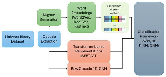
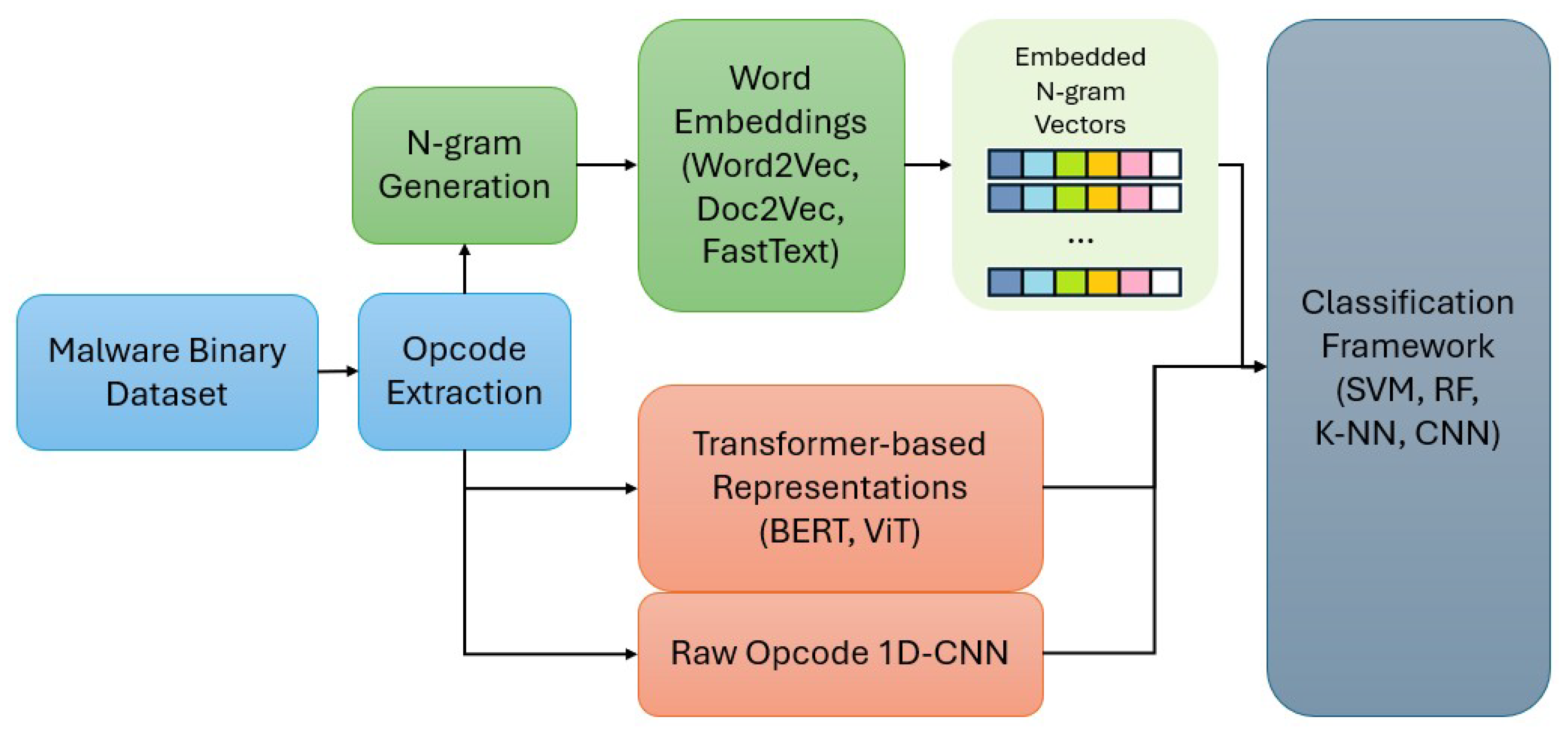
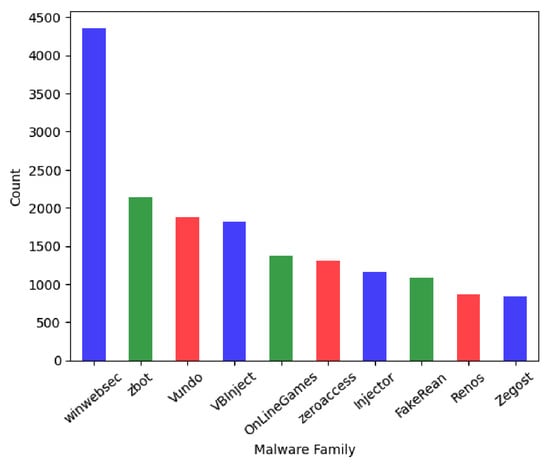
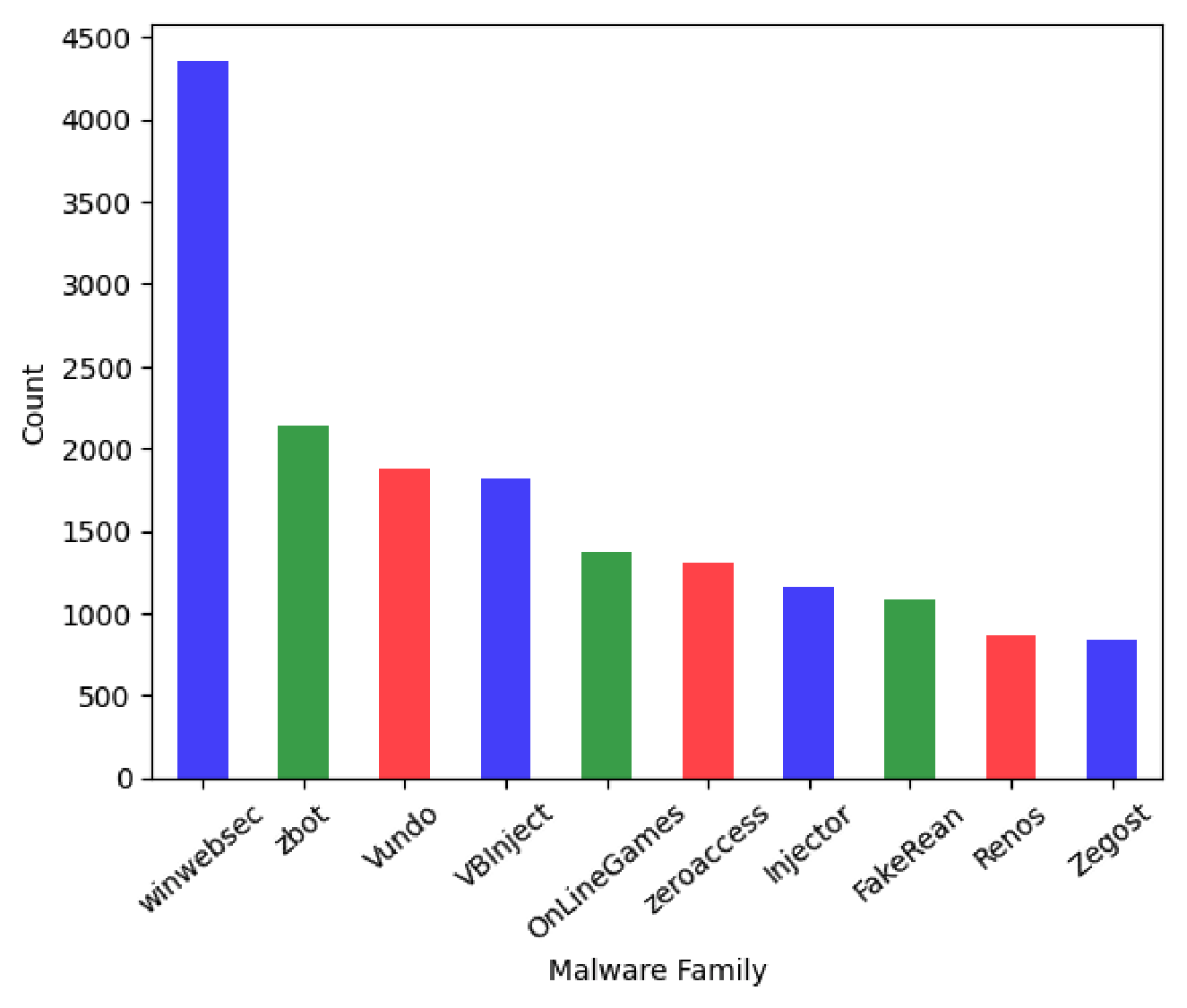
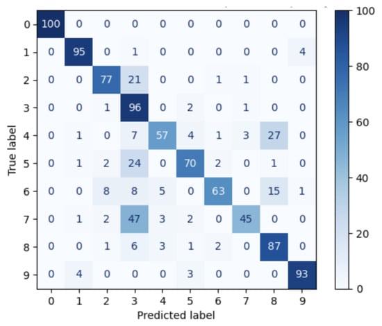
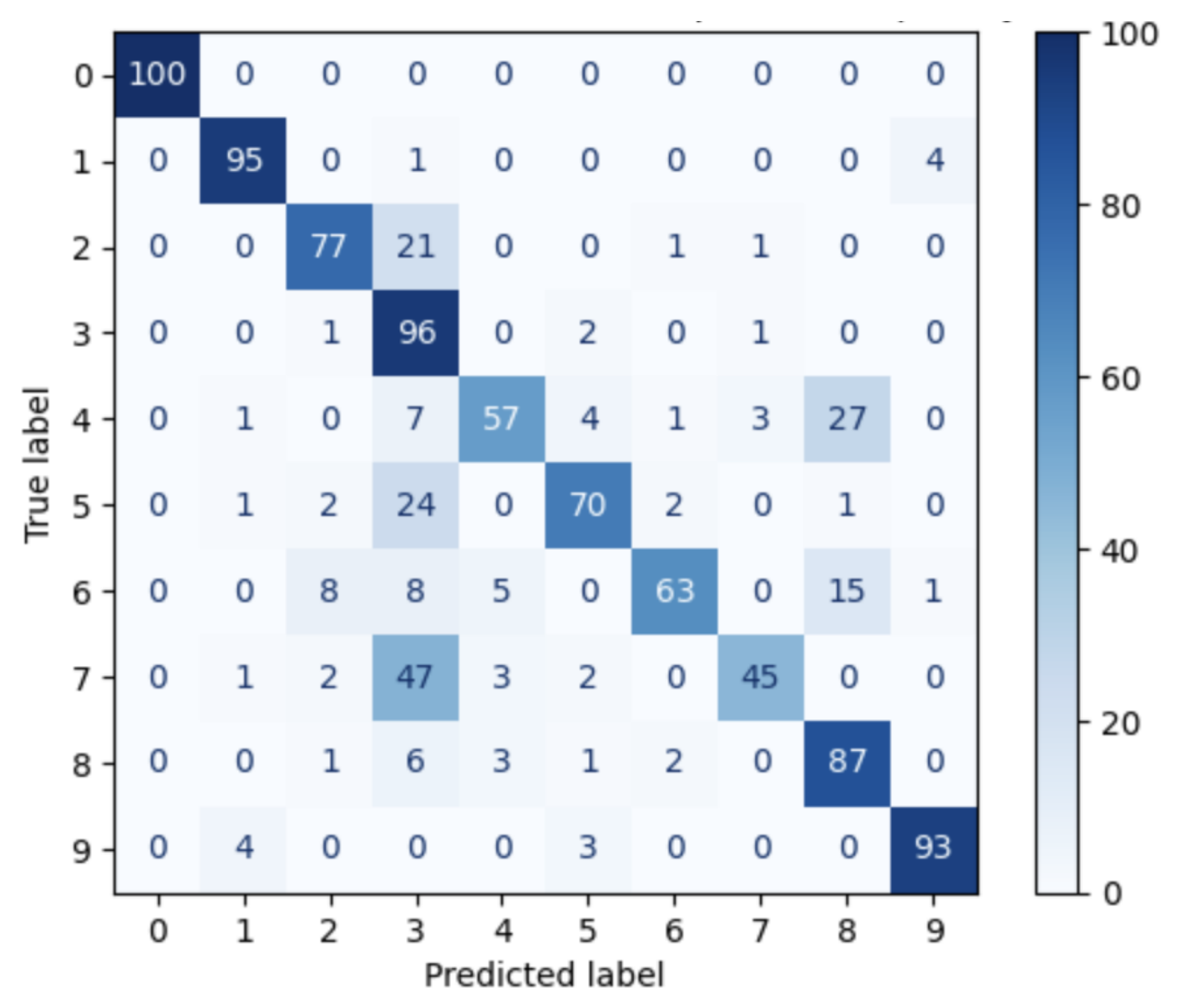
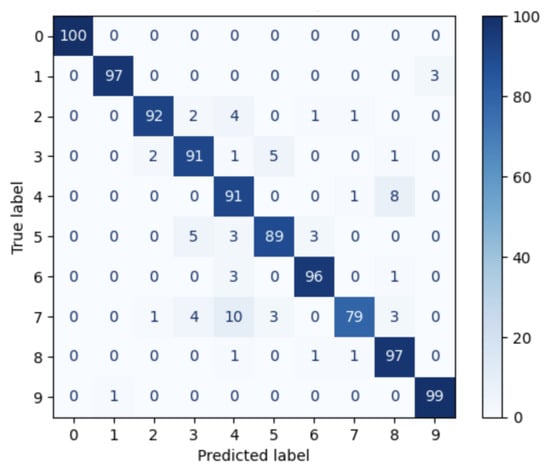
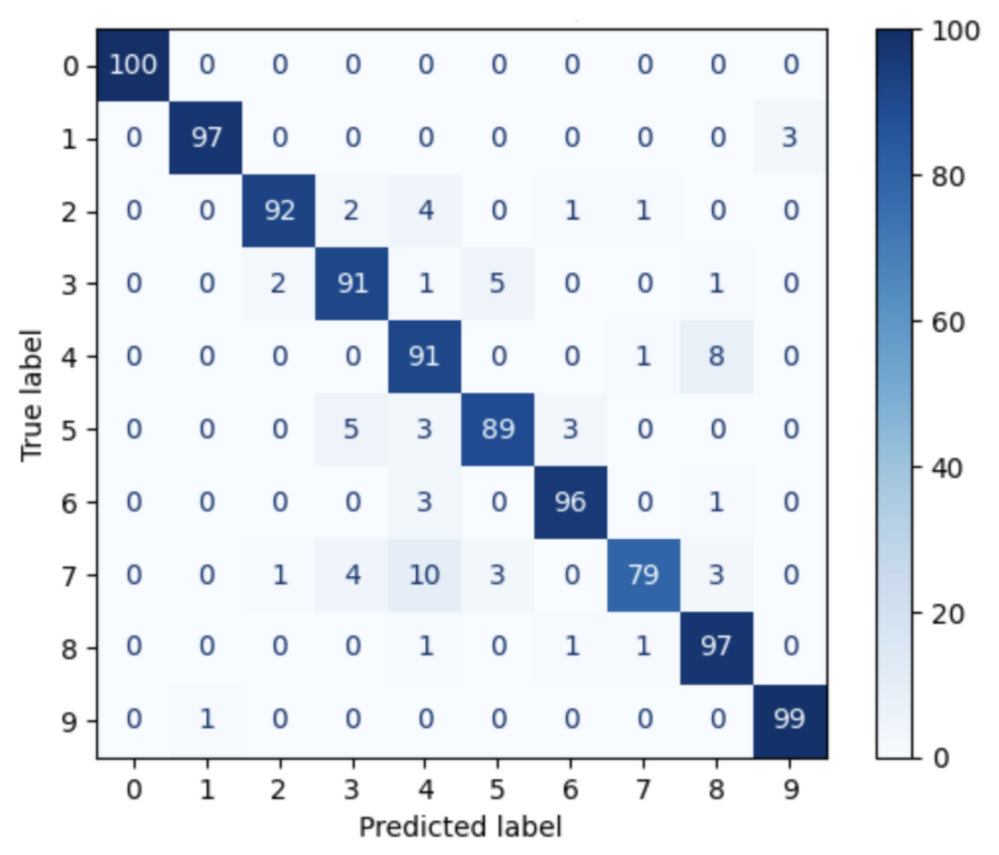
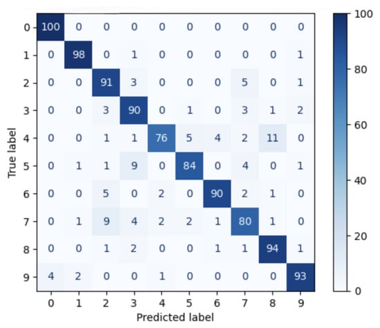
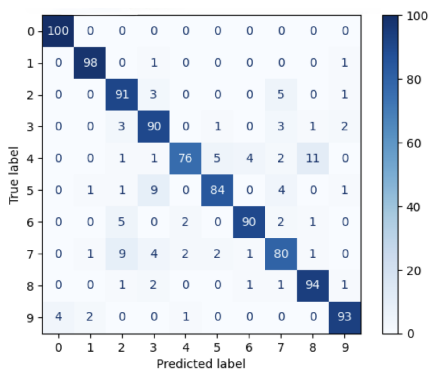
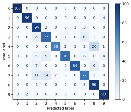
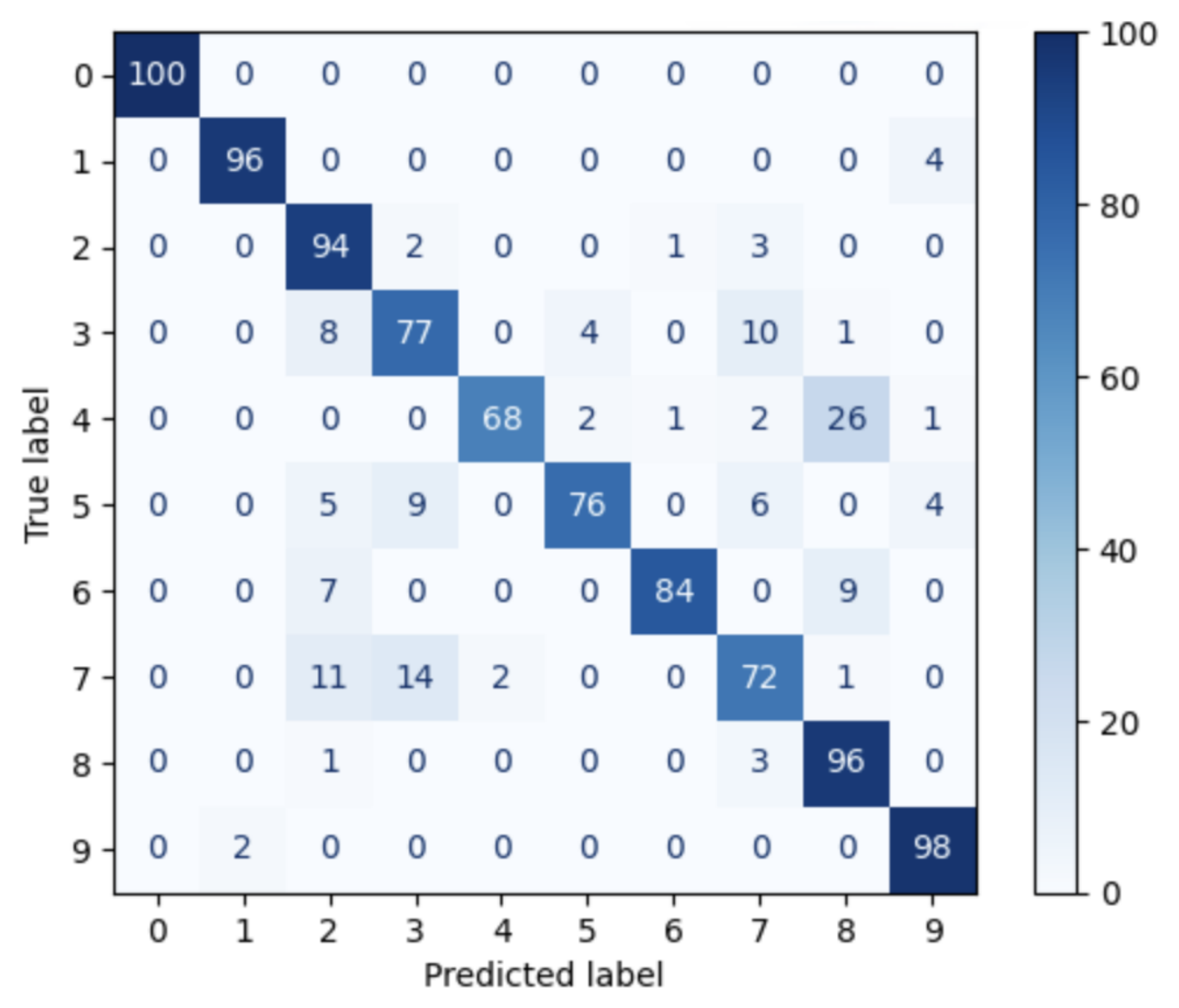
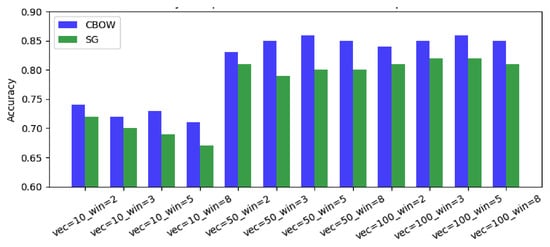
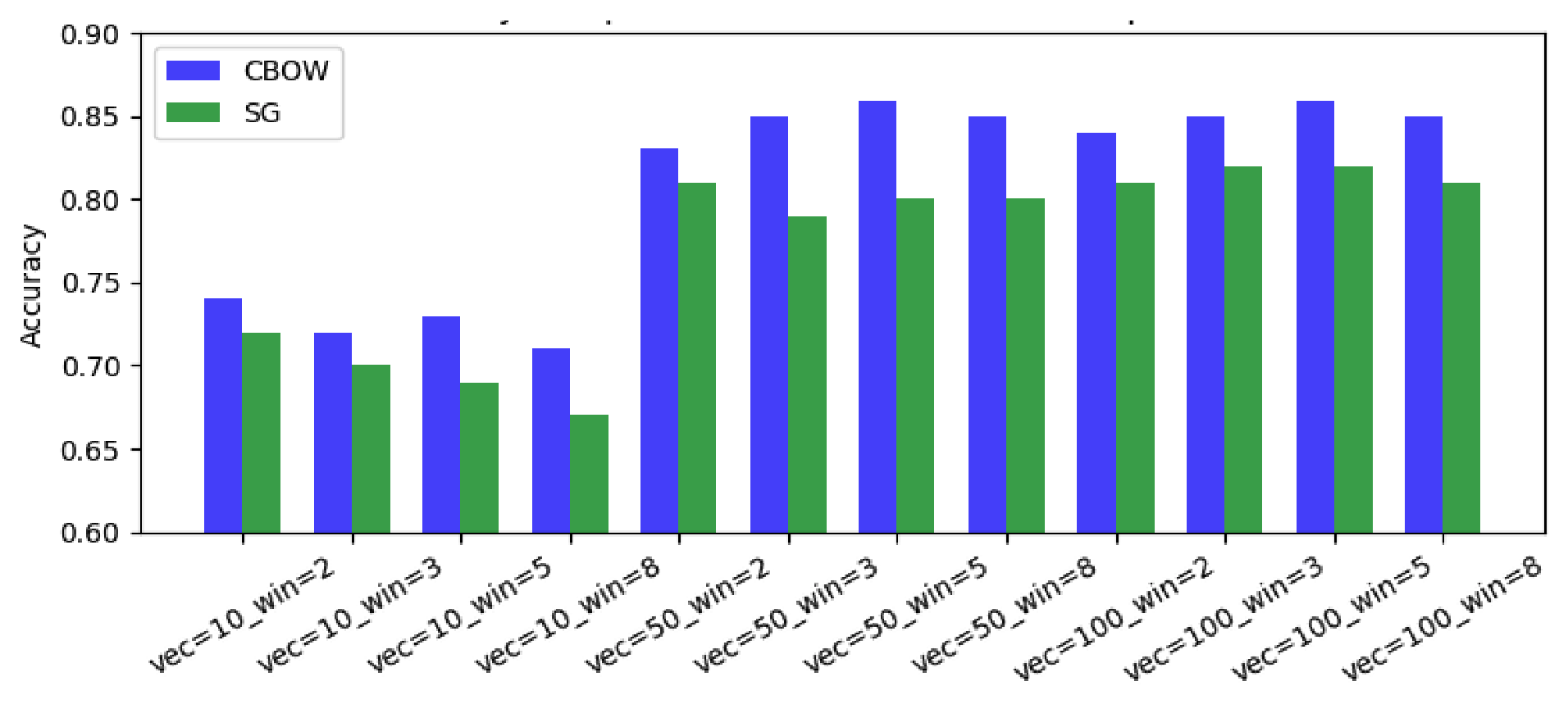
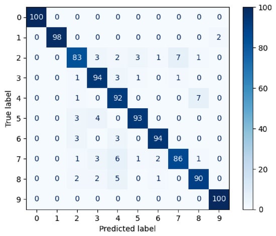
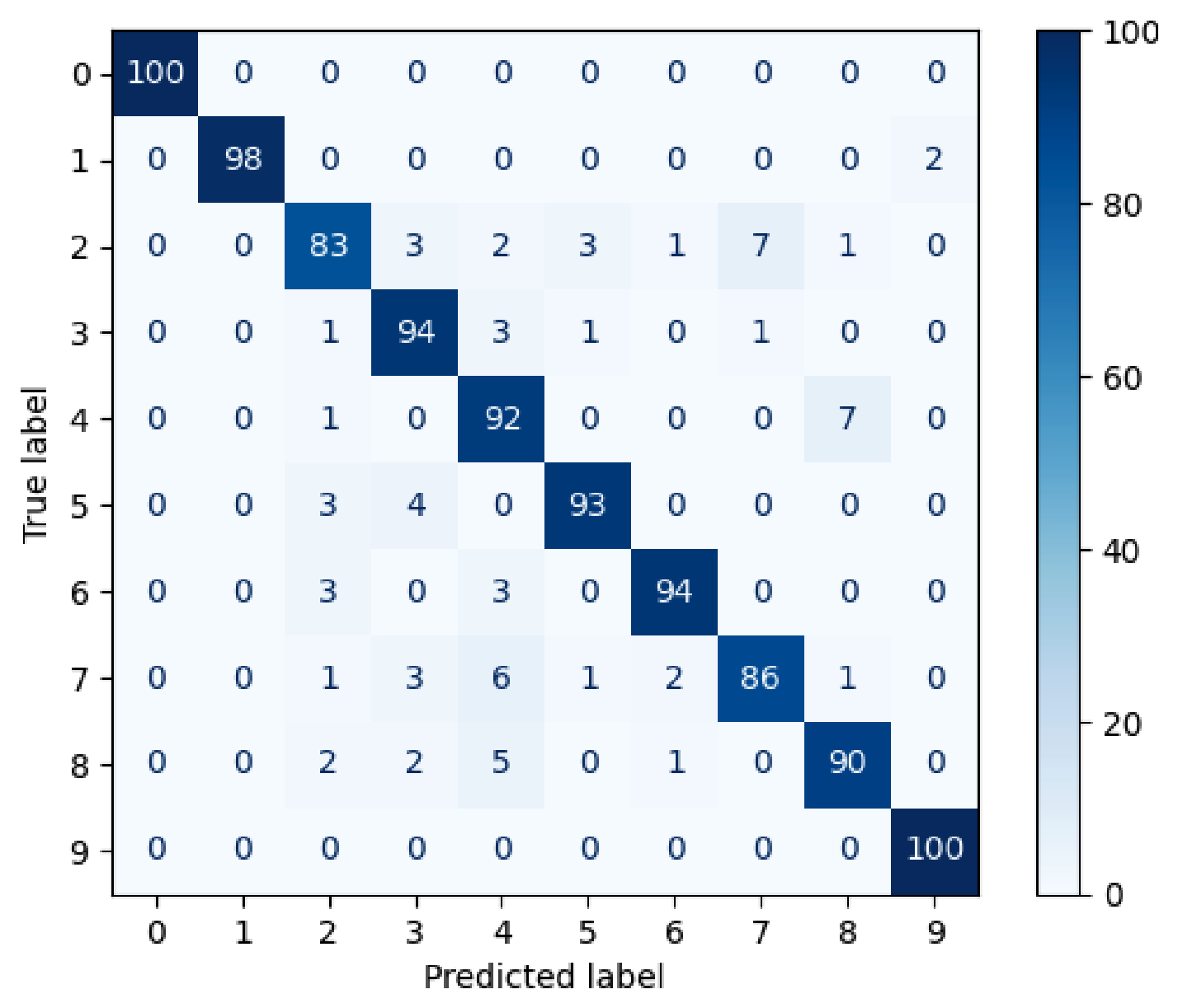
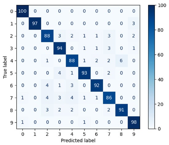
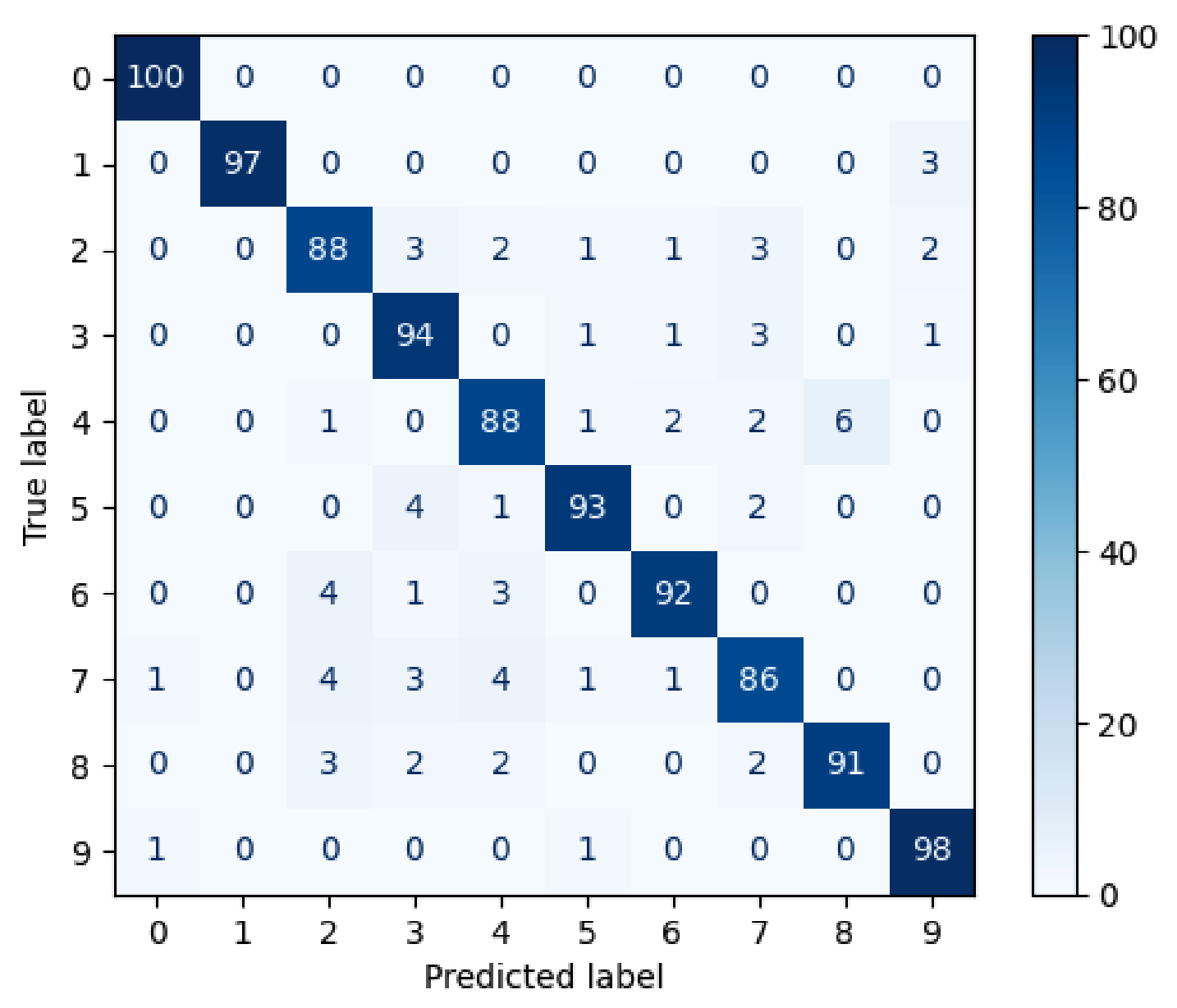
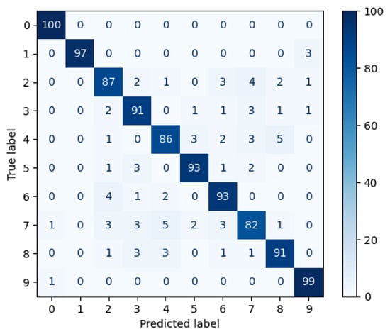
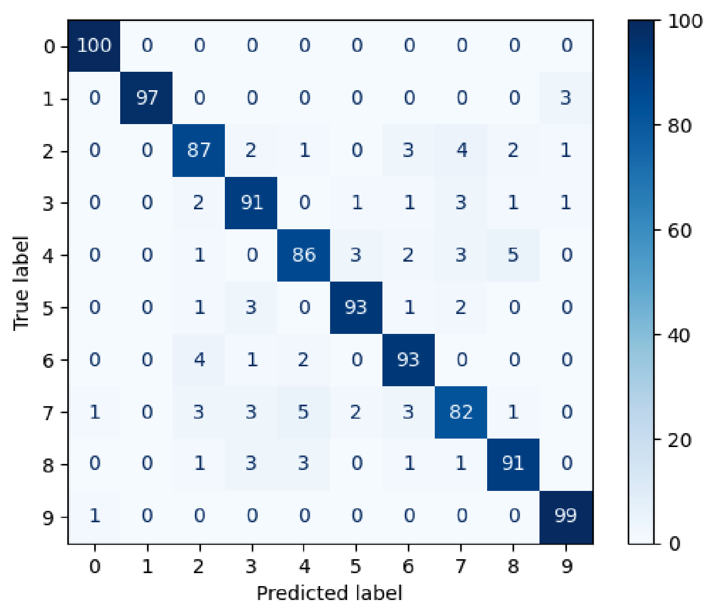
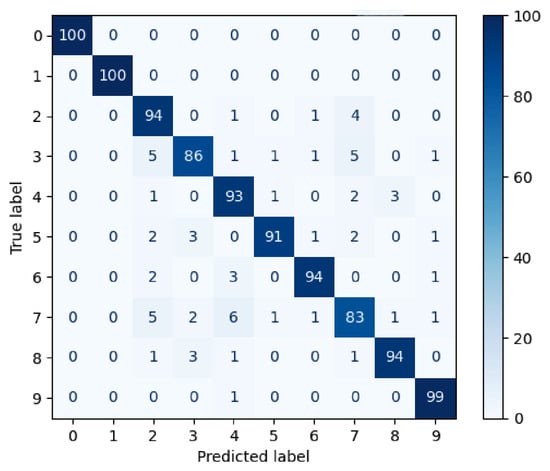
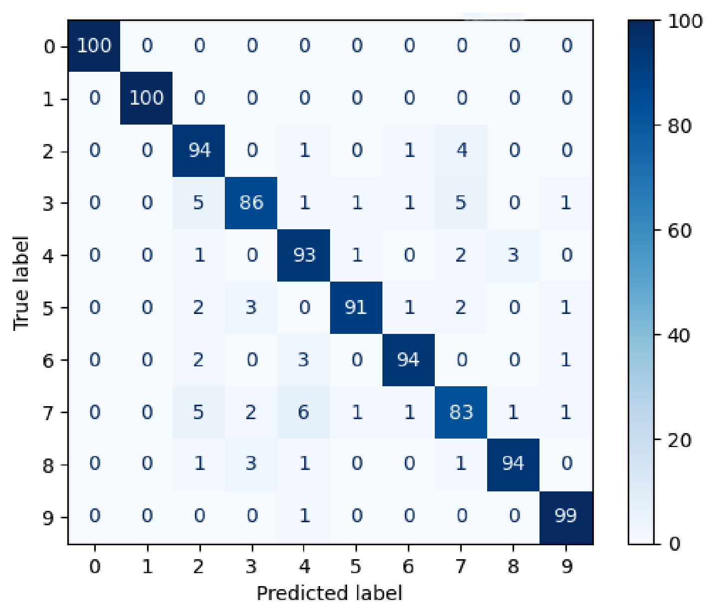
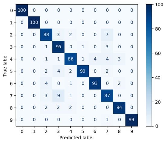
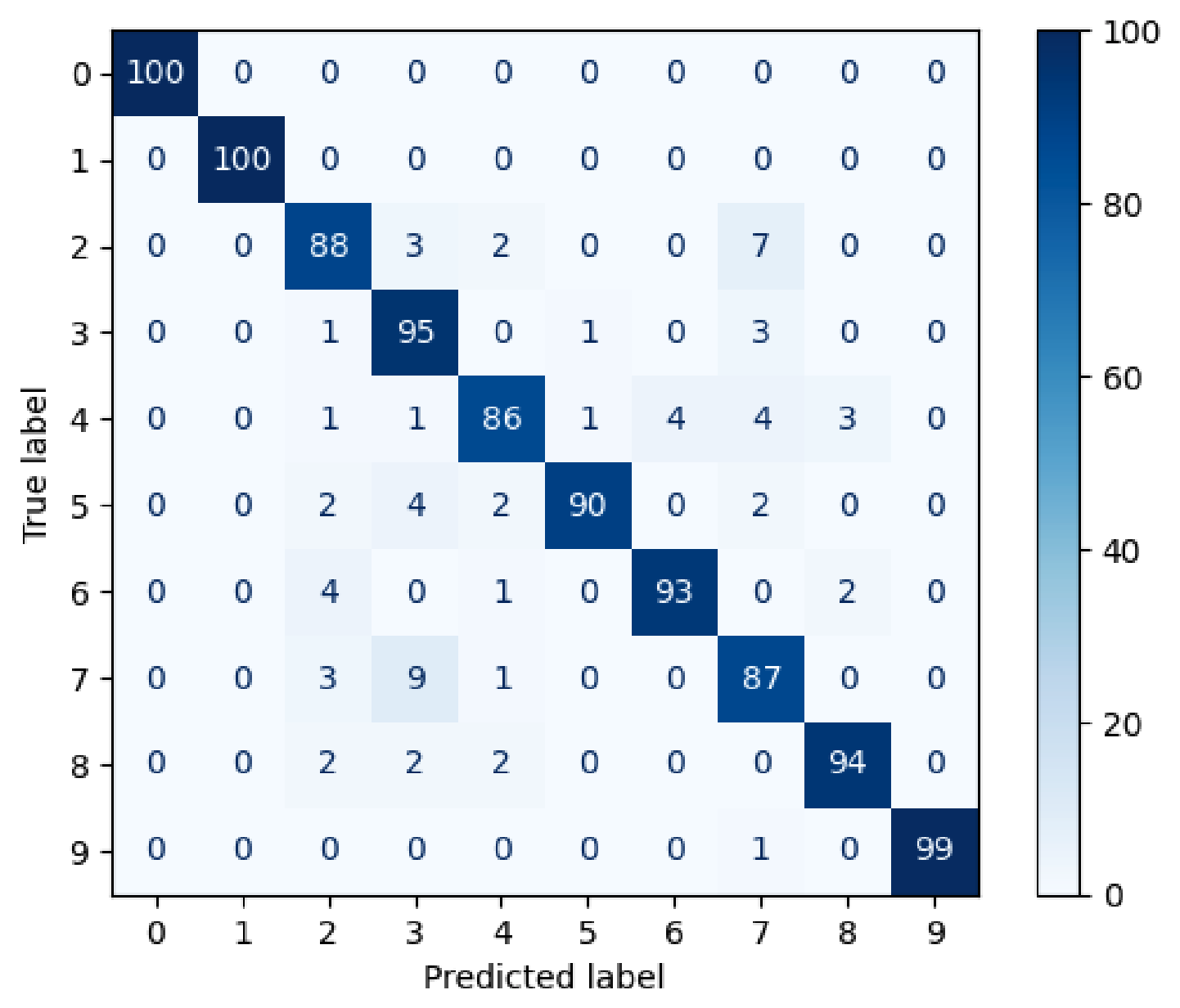
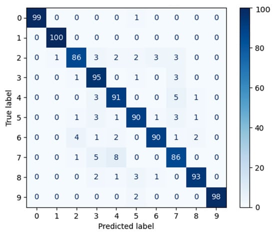
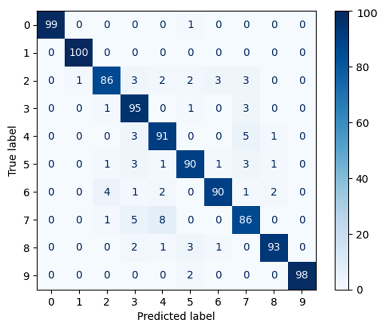
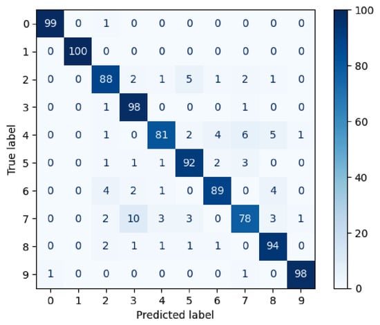
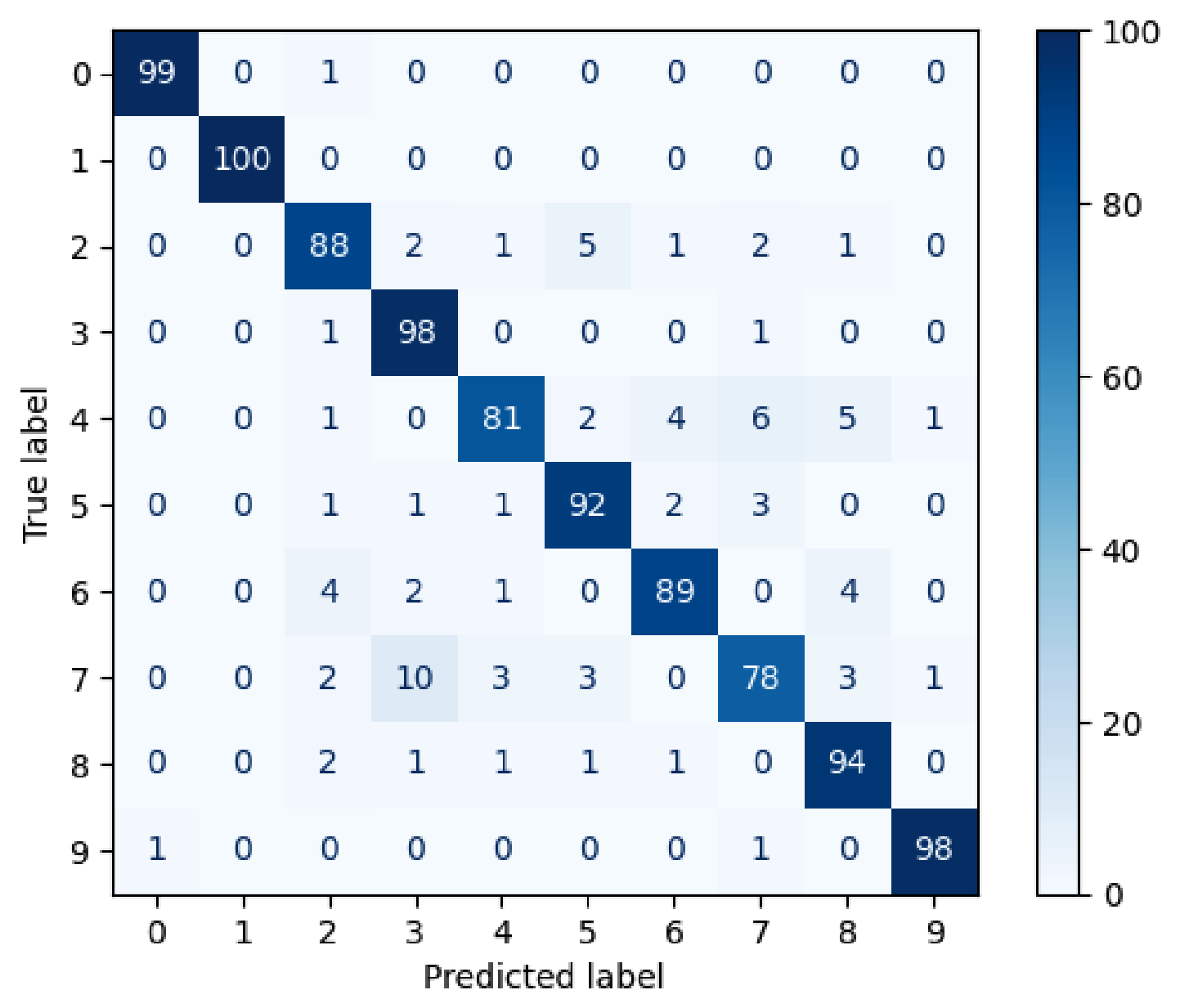
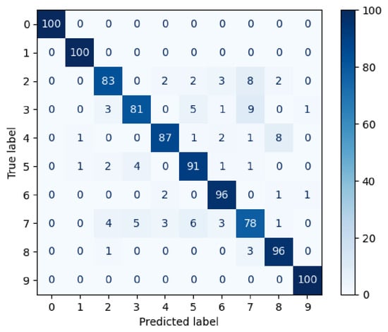
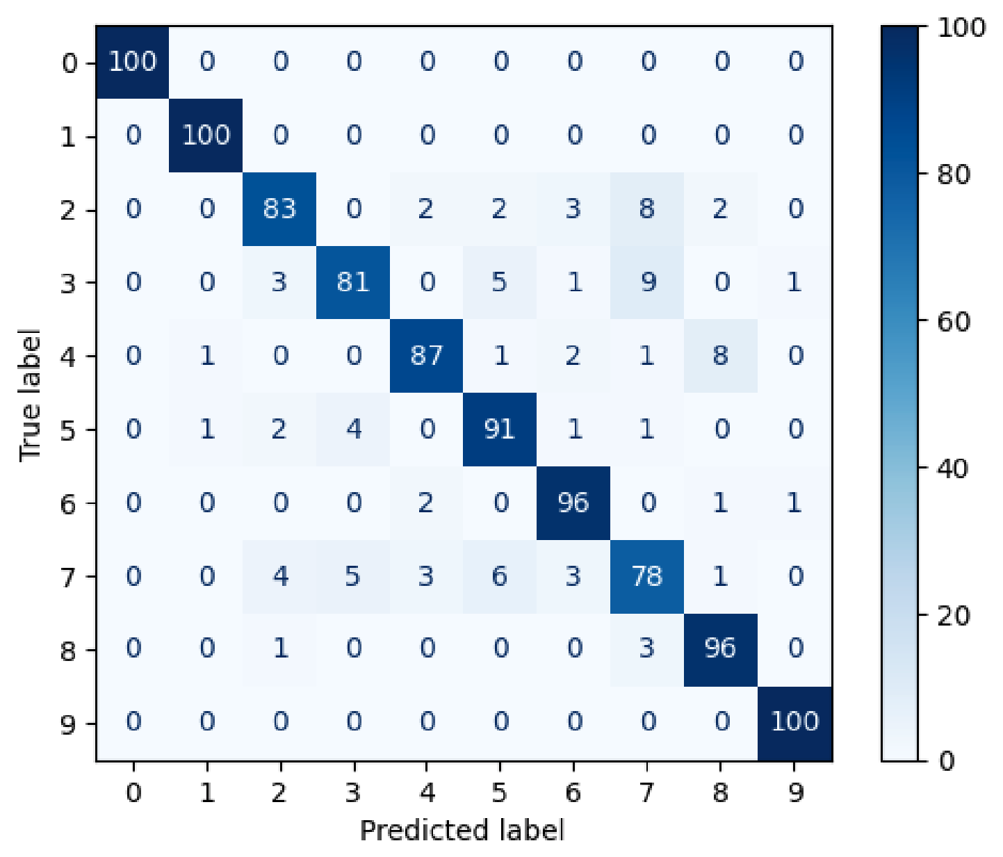
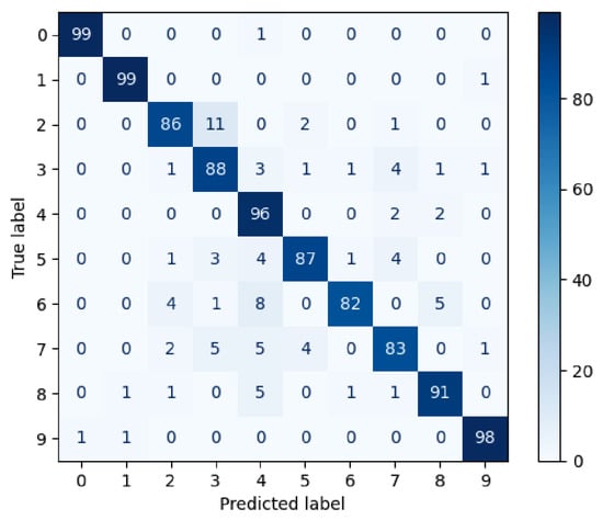
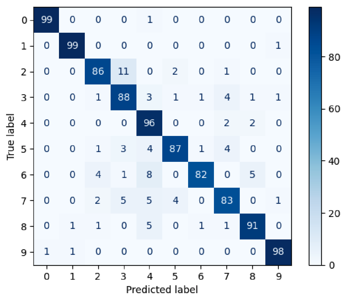
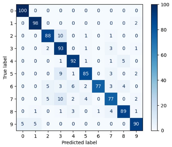
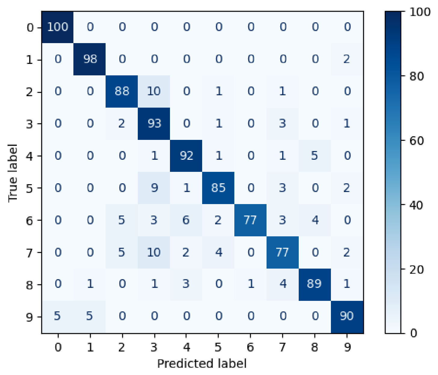
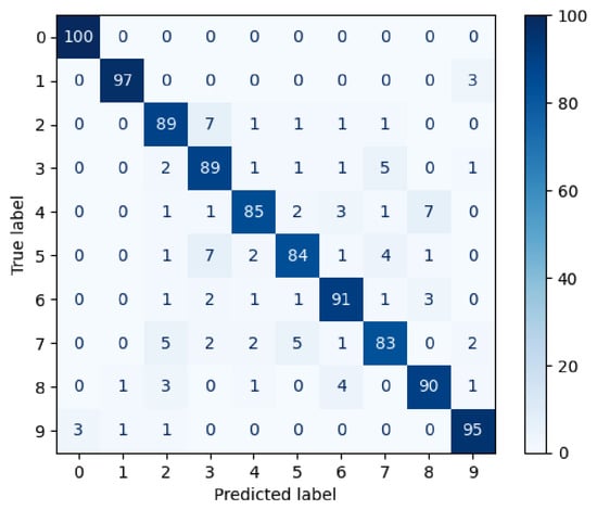
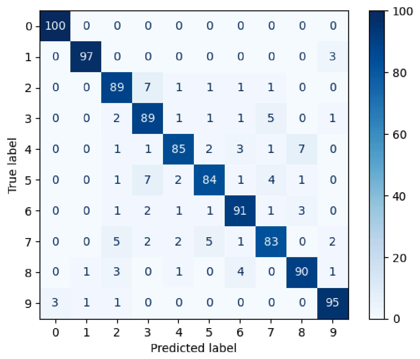
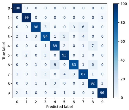
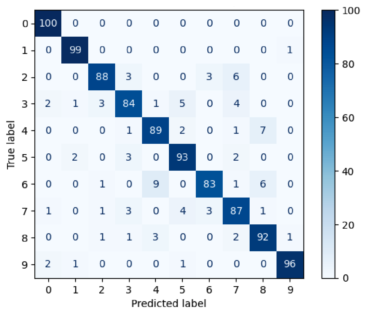
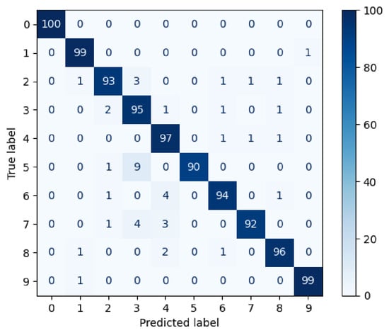
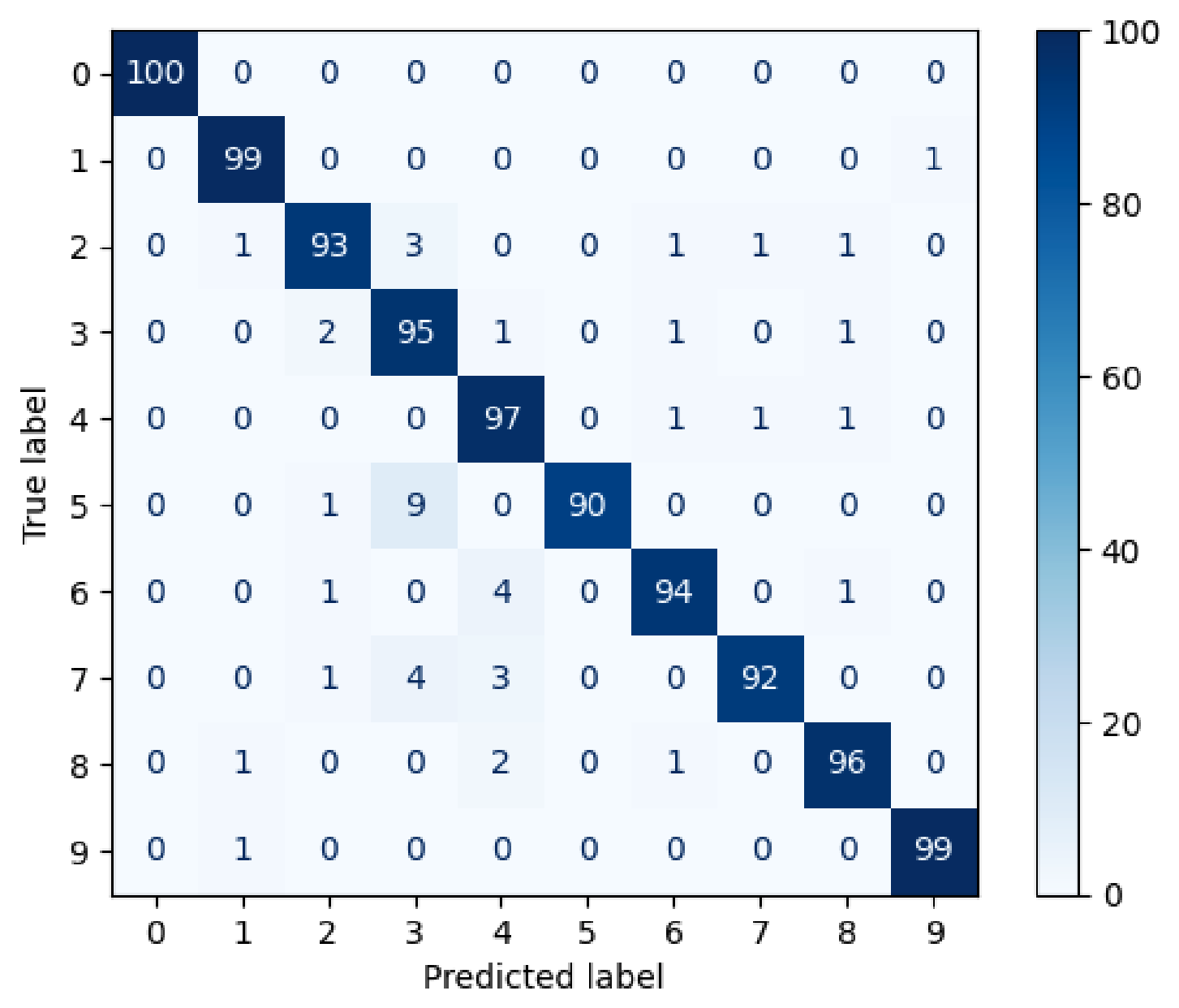
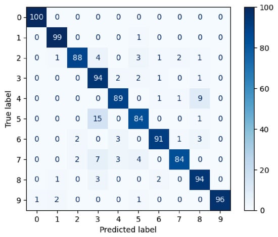
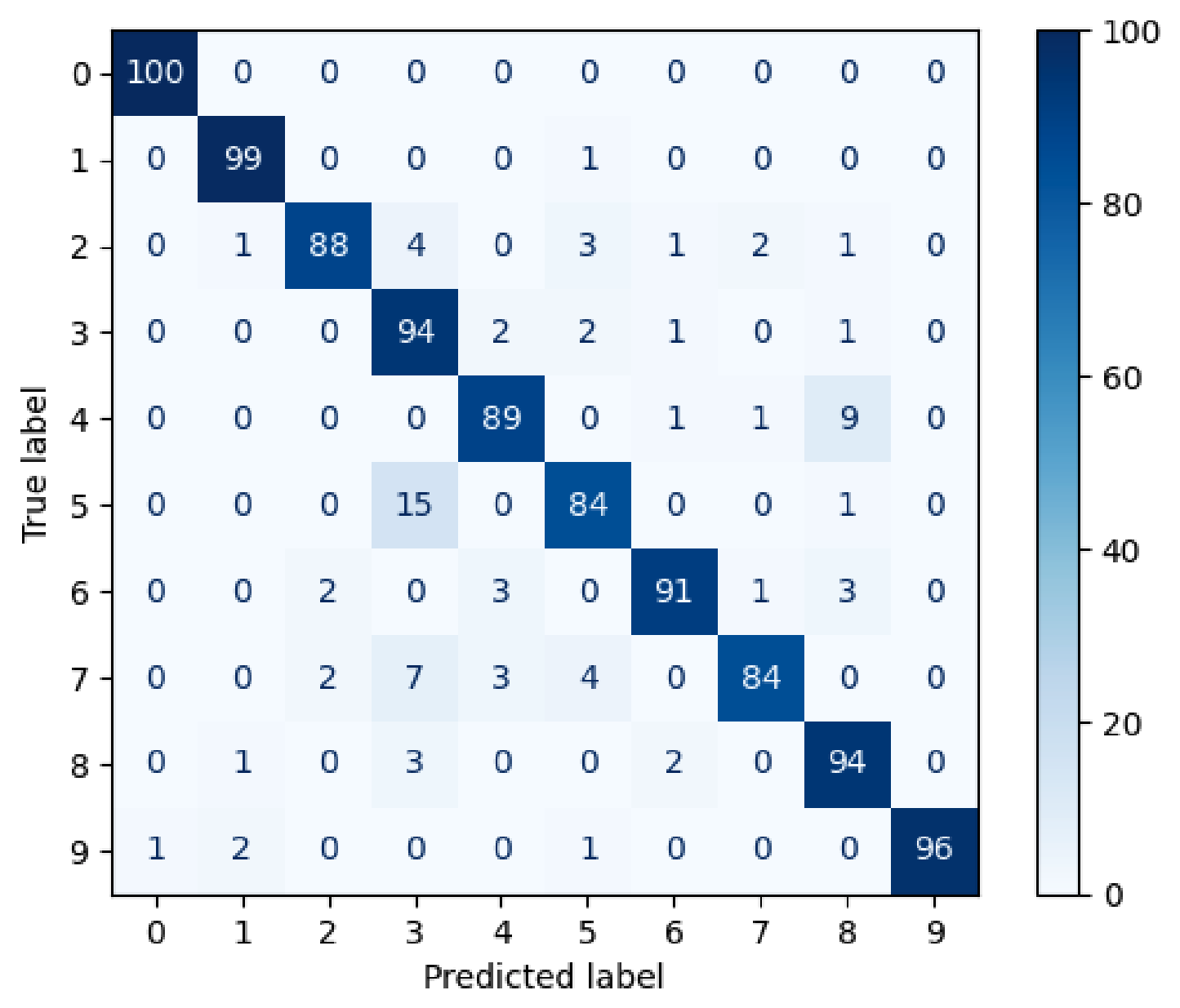
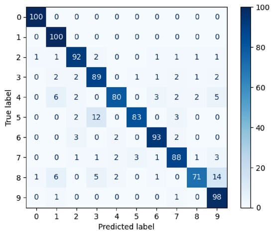
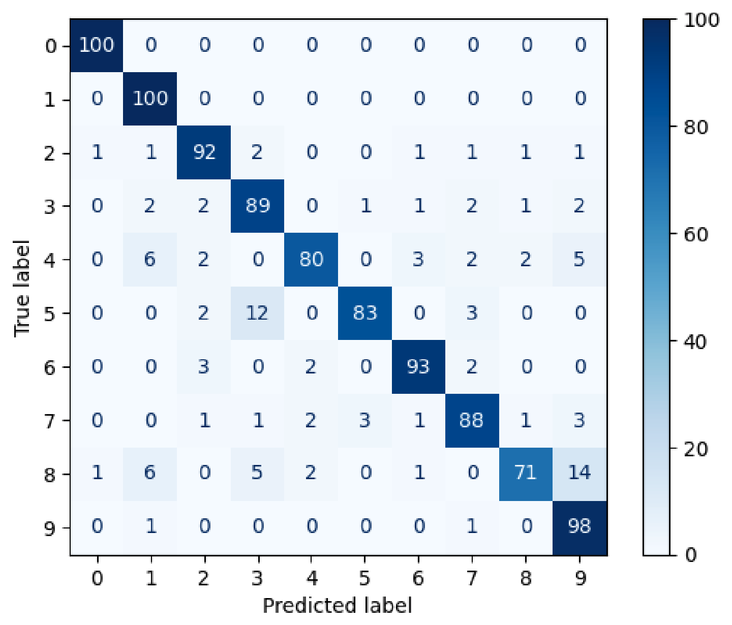
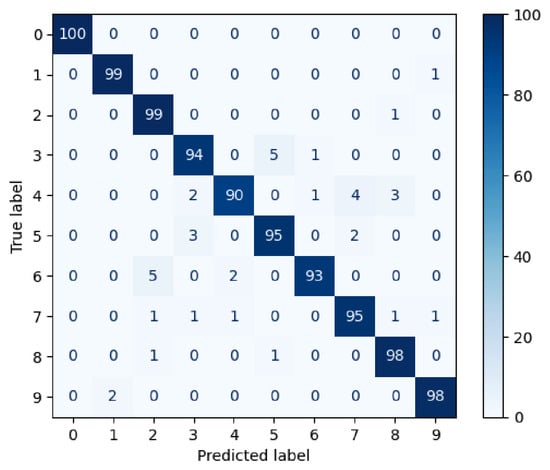
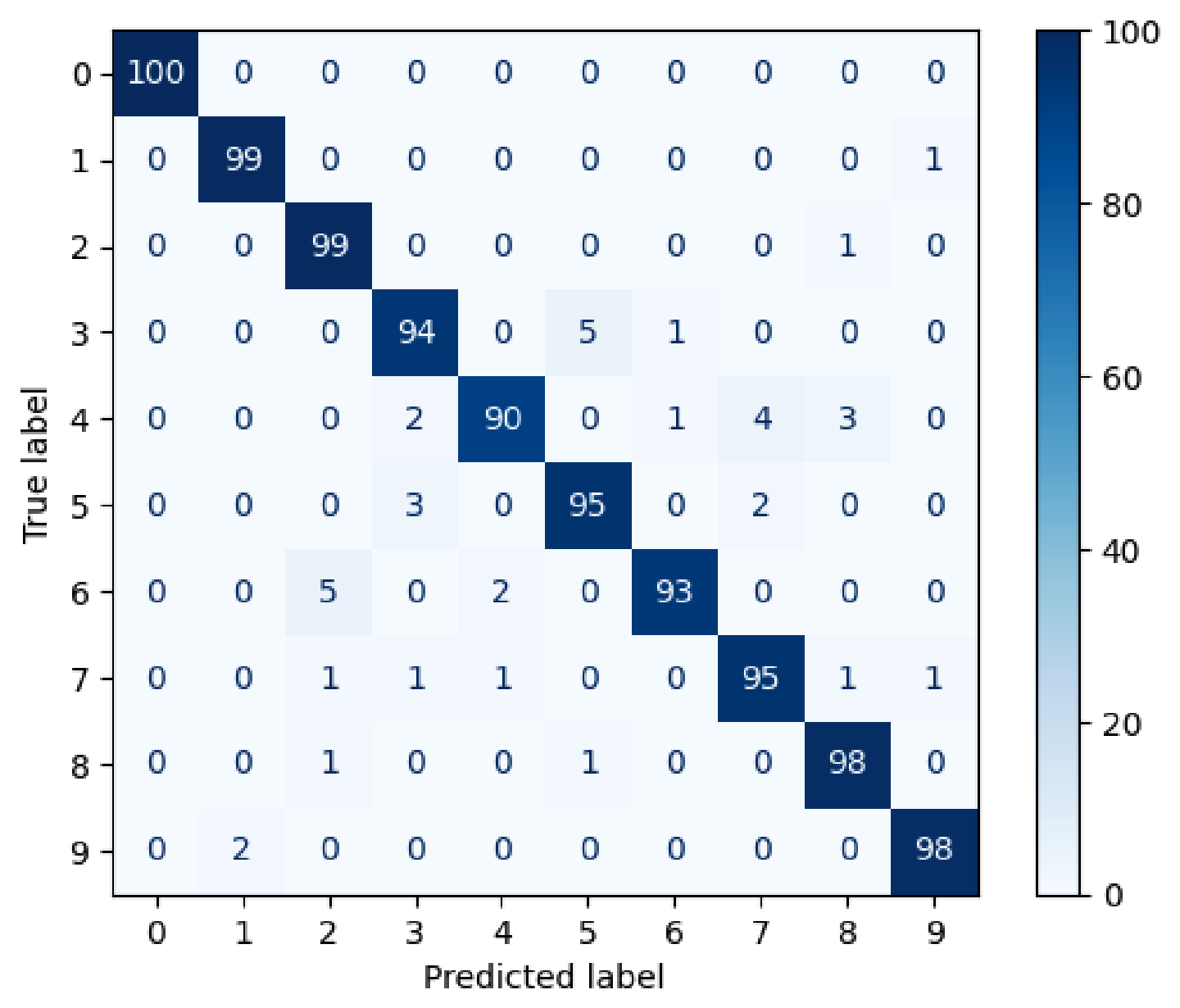
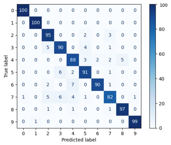
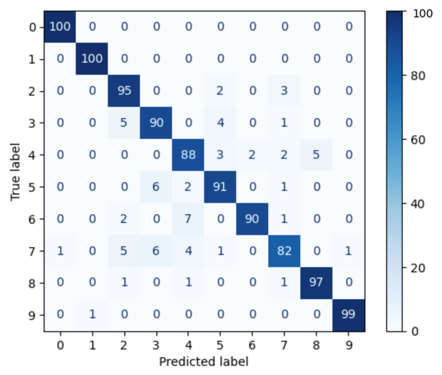
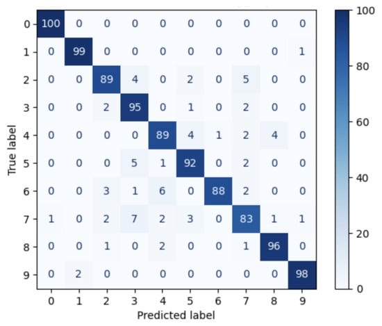
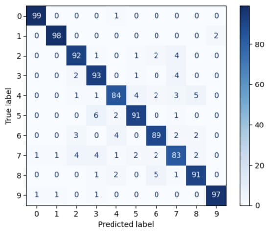
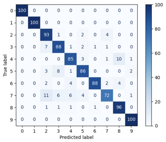
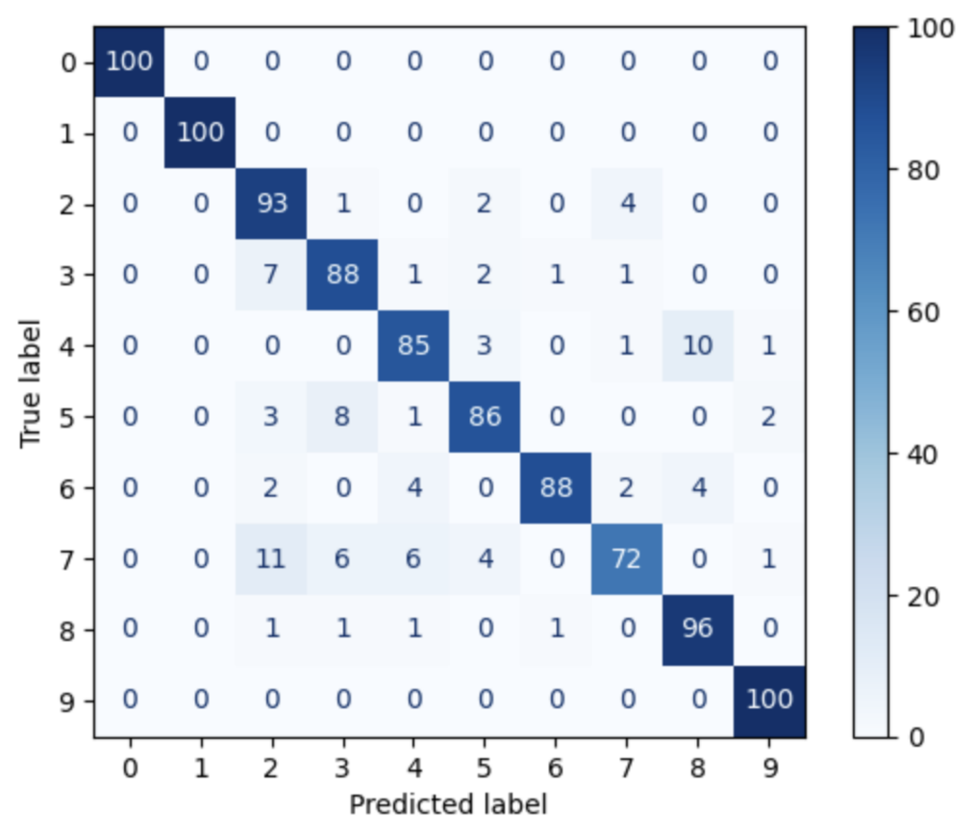
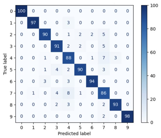
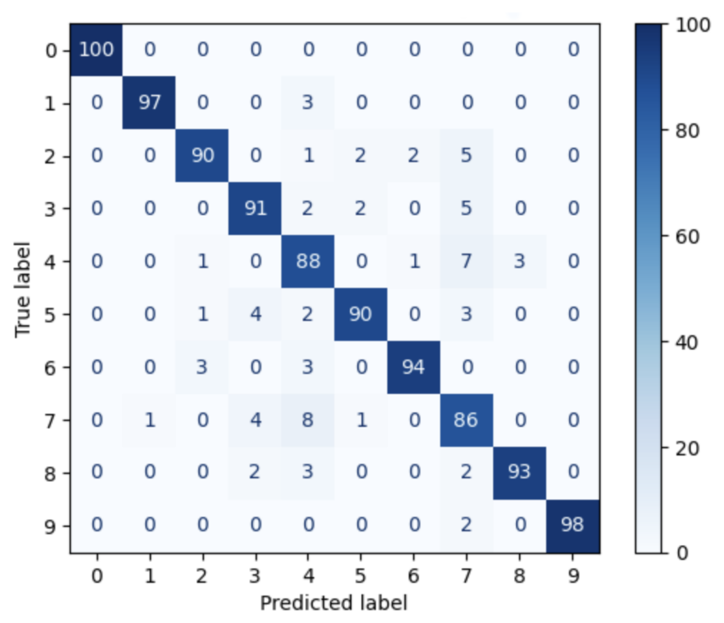
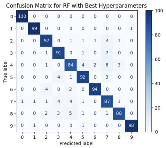
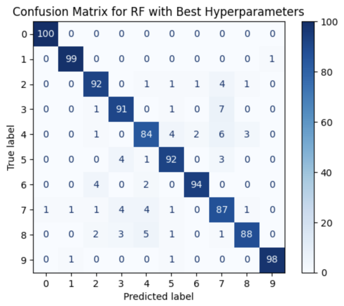
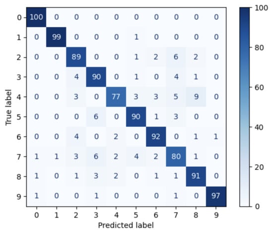
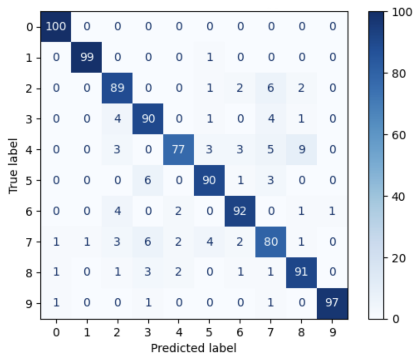
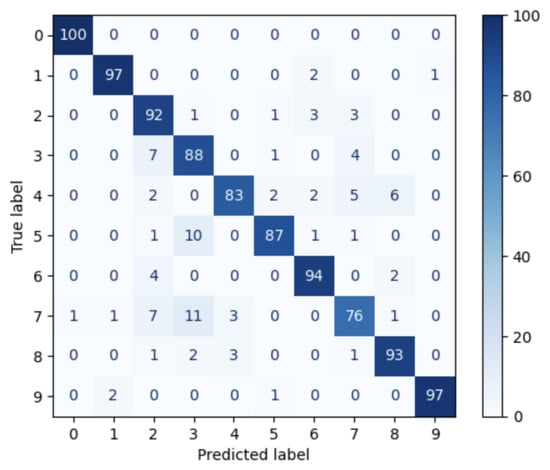
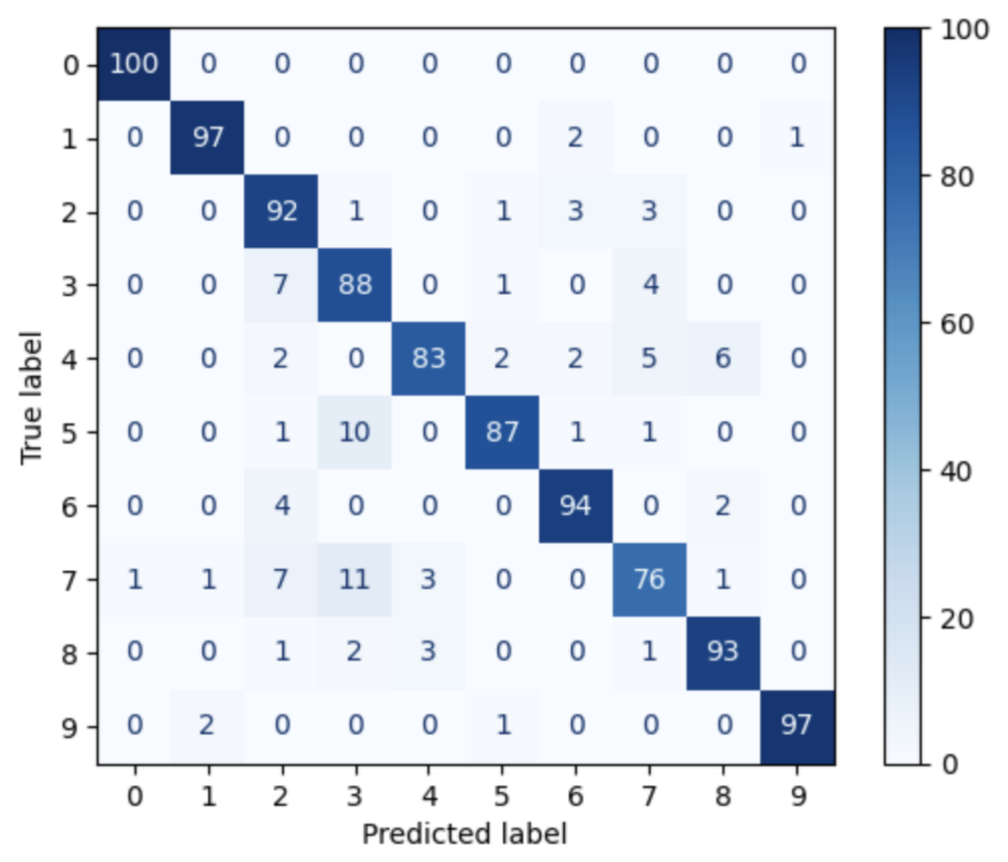
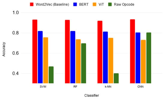
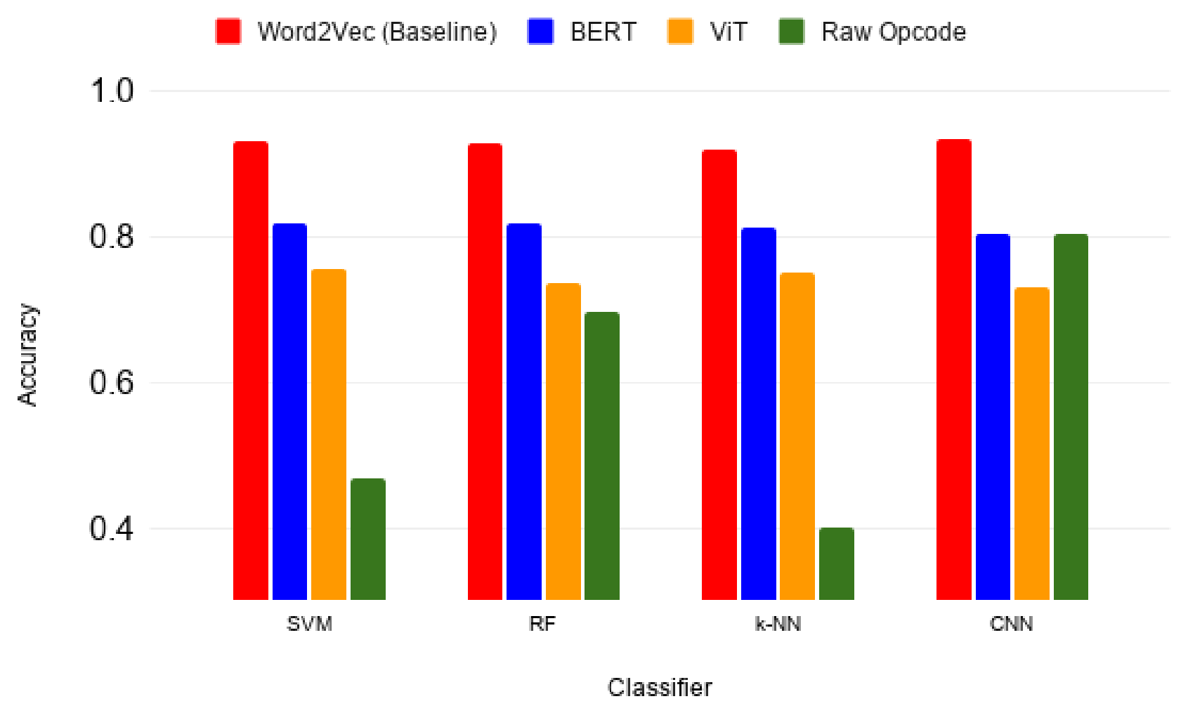
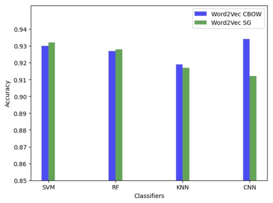
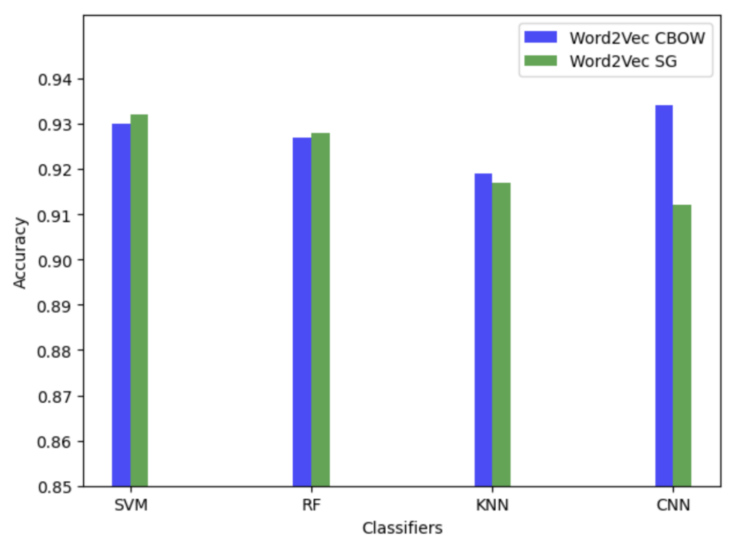
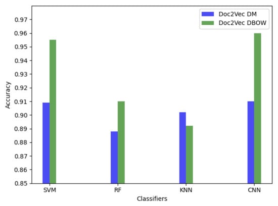
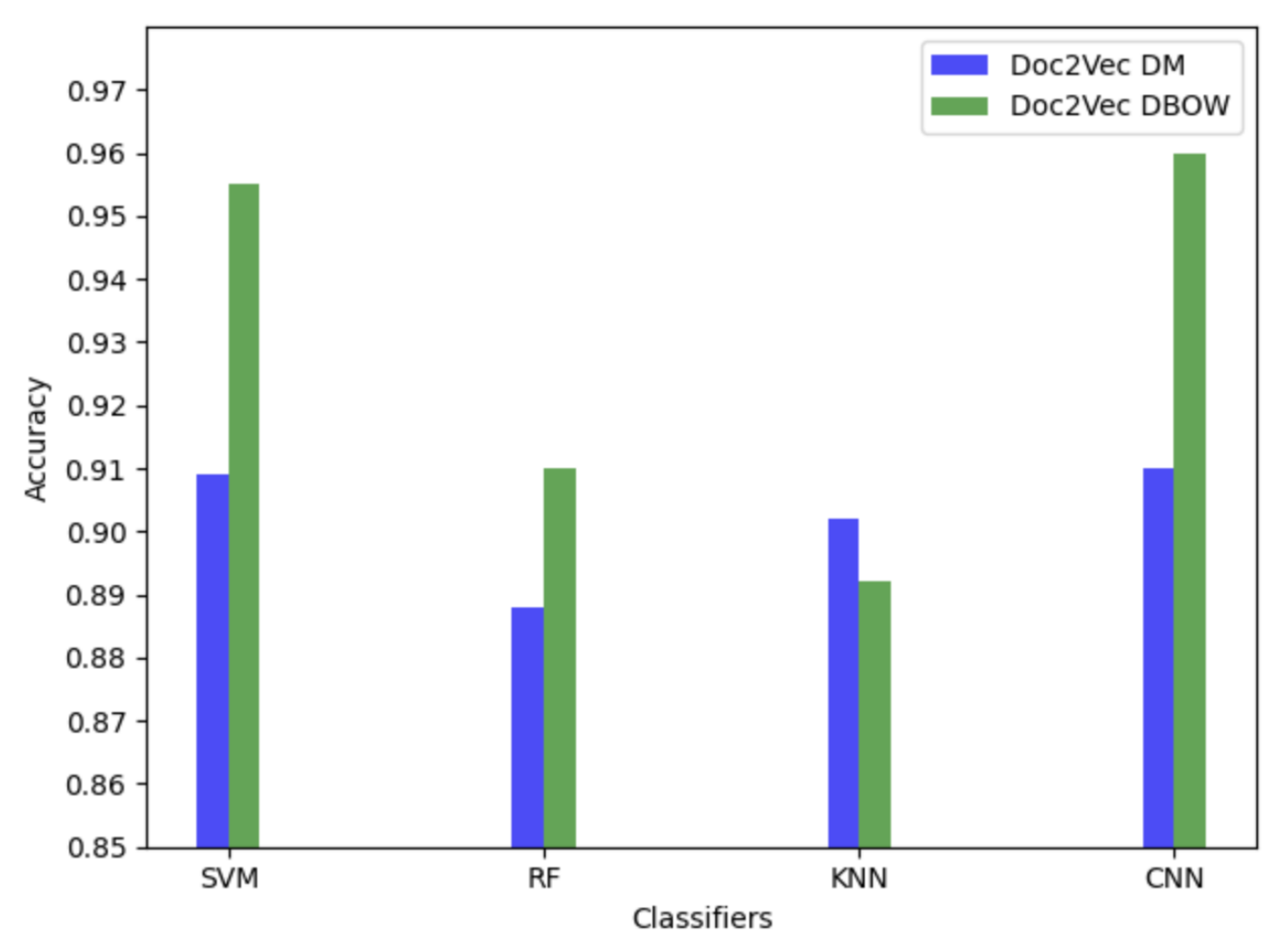
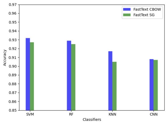
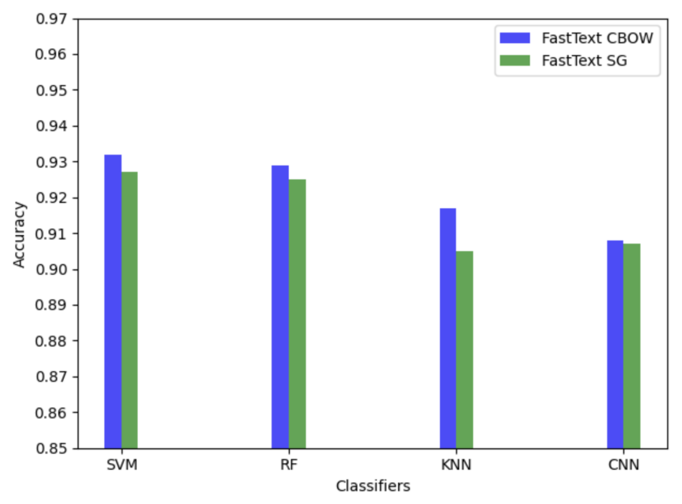
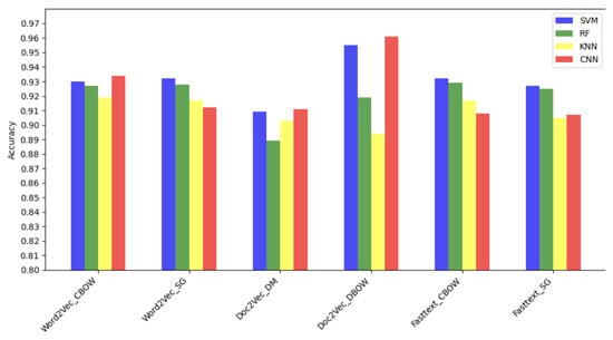
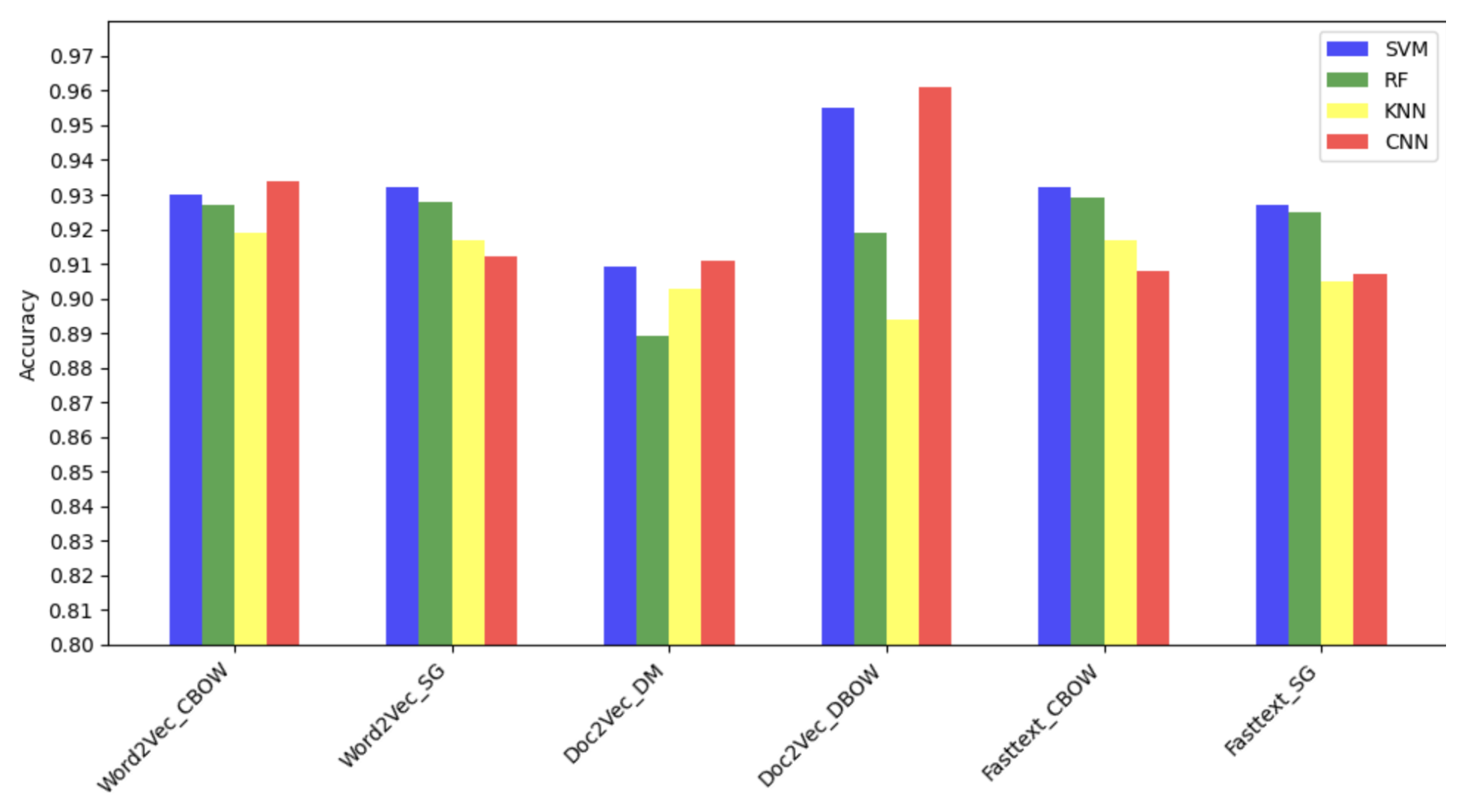

Disclaimer/Publisher’s Note: The statements, opinions and data contained in all publications are solely those of the individual author(s) and contributor(s) and not of MDPI and/or the editor(s). MDPI and/or the editor(s) disclaim responsibility for any injury to people or property resulting from any ideas, methods, instructions or products referred to in the content. |
© 2026 by the authors. Licensee MDPI, Basel, Switzerland. This article is an open access article distributed under the terms and conditions of the Creative Commons Attribution (CC BY) license.