Automated Extraction of Superconducting Qubit–Qubit Couplings from Full-Wave Multiport Impedance with Reduced-Model Analysis

Abstract

Accurate prediction of qubit–qubit exchange coupling is essential for superconducting processor design. We present and benchmark an automated full-wave electromagnetic (EM) workflow in Keysight Advanced Design System (ADS) and QuantumPro that evaluates pairwise exchange couplings from layout-level multiport responses using the established transfer-impedance relation of Solgun et al. Because many scalable superconducting processors employ repeated or near-repeated coupling motifs, reduced EM models can lower computational cost if their error is quantified. We study nearest-neighbor couplings in a reconstructed geometry based on the IBM Q 16 Rueschlikon processor using a sixteen-qubit (16Q) coupling-network model, four-qubit (4Q) unit-cell models, and pair-specific two-qubit (2Q) sub-blocks. The 4Q models provide a like-for-like external benchmark because they match the model extent used by Solgun et al. for the published full-wave coupling calculations. The 4Q models reproduce the published simulated couplings with a 3.70% mean absolute percentage error and differ from 16Q by 3.62% on average. For the representative single solves reported here, the 16Q solve takes approximately 7.2 times as long as 4Q and requires 5.7 times the peak memory. This supports 4Q as a practical reduced model for quantitative local coupling prediction. Further reduction to 2Q changes the couplings by 6.17% on average but remains effective for inexpensive mesh-convergence screening. The resulting workflow provides automated exchange-coupling extraction together with model-extent and convergence assessment in a commercial microwave EDA environment.

1. Introduction

Superconducting circuits are a leading platform for quantum information processing, owing to their scalability and compatibility with planar microwave technology [1,2,3]. As the number of qubits grows and gate fidelities continue to improve, circuit-level engineering of the surrounding electromagnetic (EM) environment becomes central to reliable multiqubit operation.

For two qubits coupled through a shared resonator, or more generally through a linear microwave environment, the exchange coupling $J_{ij}$ sets the characteristic interaction rate between qubits i and j and therefore the timescale of exchange-based two-qubit operations [4]. In multiqubit devices, the coupled environment and applied drives can also produce unwanted static or drive-activated interactions and crosstalk [5,6,7,8,9]. Strong interactions can enable faster entangling operations, but residual $ZZ$ coupling and spectator/crosstalk errors must also be controlled [10,11]. Designing for high-fidelity two-qubit operation therefore calls for predictive, quantitative modeling of $J_{ij}$ at the design stage.

For processor layouts with distributed microwave structures, a purely lumped description can miss critical multimode electromagnetic behavior [12]. An additional difficulty is that $J_{ij}$ arises from the interplay between the nonlinear Josephson junctions and the distributed linear EM environment. Several complementary approaches bridge classical EM models and effective quantum descriptions. For example, black-box quantization constructs a low-energy Hamiltonian from the modes of the linearized environment [12], while energy-participation-ratio analysis extracts Hamiltonian, participation, and dissipation parameters from eigenmode solutions [13]. Unlike these methods, which provide broader modal and Hamiltonian information, the impedance-response formulation of Solgun et al. directly targets selected pairwise exchange couplings by relating them to off-diagonal entries of the multiport impedance matrix defined at the junction ports [14] and is referred to hereafter as the Solgun method. This method has also been extended to evaluate $ZZ$ interaction rates [15].

Recent efforts have also addressed the broader integration of EM simulation and automated parameter extraction into superconducting-circuit design, including full-wave 3D quantum-parameter extraction in EMPro [16], the QuantumPro environment in Keysight ADS [17], the SQuADDS design database and simulation workflow [18], and scalable open-source EM workflows [19]. Forati et al. [20] discuss electromagnetic coupling definitions and connect them to the practical extraction of coupling parameters from full-wave EM simulations. Full-wave impedance-based exchange-coupling extraction has also been demonstrated for smaller multiqubit transmon structures by Khan and Roth [21]. Levenson-Falk and Shanto [22] review the broader design challenges in superconducting quantum circuits, including the connection between physical layout, electromagnetic simulation, quantum circuit parameters, and system-level device performance.

Full-wave EM analysis is therefore well suited to analyzing qubit–qubit exchange couplings, but its computational cost rises rapidly with model extent. Many scalable superconducting processors, however, reuse identical or nearly identical unit cells. This motivates a central question of this work: how far can the EM model of a superconducting processor layout be reduced for early design and convergence studies while retaining useful accuracy in nearest-neighbor couplings?

In this work, we present and benchmark an automated layout-level J-extraction workflow in Keysight Advanced Design System (ADS) 2027 with QuantumPro using the Solgun method. We first apply the workflow to the reconstructed four-qubit unit-cell models (4Q), matching the model extent used by Solgun et al. [14] and providing the external benchmark for the present study. We then use the same reconstruction to construct a sixteen-qubit coupling-network model (16Q) and pair-specific two-qubit sub-blocks (2Q) to investigate the model-reduction question posed above. Whereas Solgun et al. [14] restricted their detailed full-wave coupling calculations to $2\times 2$ four-qubit unit cells because of the available memory resources, the present workflow directly solves a single 16Q coupling-network model and extracts pairwise exchange couplings from its multiport EM response. To the best of our knowledge, this is the first reported application of full-wave multiport-impedance-based exchange-coupling extraction to a single 16-transmon coupling-network model. We examine agreement with the published benchmark, the effects of model reduction, and numerical convergence.

The remainder of the paper is organized as follows. Section 2 describes the 16Q, 4Q, and 2Q EM models and the automated full-wave coupling-extraction workflow, including the port definitions and meshing strategy. Section 3 presents the convergence study, comparison with the published benchmark, model-reduction accuracy, and computational cost. Section 4 interprets the practical roles and limitations of the three model extents. Detailed numerical results are provided in Appendix A.

2. Materials and Methods

2.1. Impedance-to-Coupling Extraction

Under the dispersive-regime assumptions of the Solgun method [14], the exchange coupling is obtained from the linearized transfer impedance as

$$J_{ij}=-{\displaystyle \frac{1}{4}}\sqrt{{\displaystyle \frac{{\omega }_i{\omega }_j}{L_i{L}_j}}}\mathrm{Im}\left[{\displaystyle \frac{Z_{ij}\left({\omega }_i\right)}{{\omega }_i}}+{\displaystyle \frac{Z_{ij}\left({\omega }_j\right)}{{\omega }_j}}\right],$$

(1)

where ${\omega }_i$ and ${\omega }_j$ are the qubit angular frequencies, $L_i$ and $L_j$ are their effective linearized inductances, and $Z_{ij}$ is the off-diagonal transfer impedance of the linear environment.

The effective linearized inductances $L_i$ used in this paper are obtained from the single-qubit parameters reported by Solgun et al. [14] and are held fixed across the 2Q, 4Q, and 16Q model extents. Their calculation and the values used for all 16 qubits are given in Appendix A and Table A1. Throughout the numerical tables and figures, coupling values are reported as $\left|J_{ij}\right|/2\pi$ in MHz.

2.2. Automated Coupling-Extraction Workflow

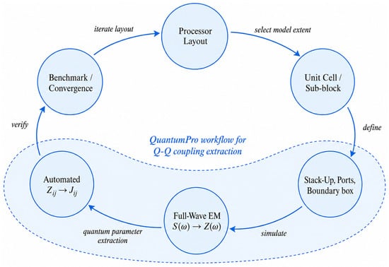
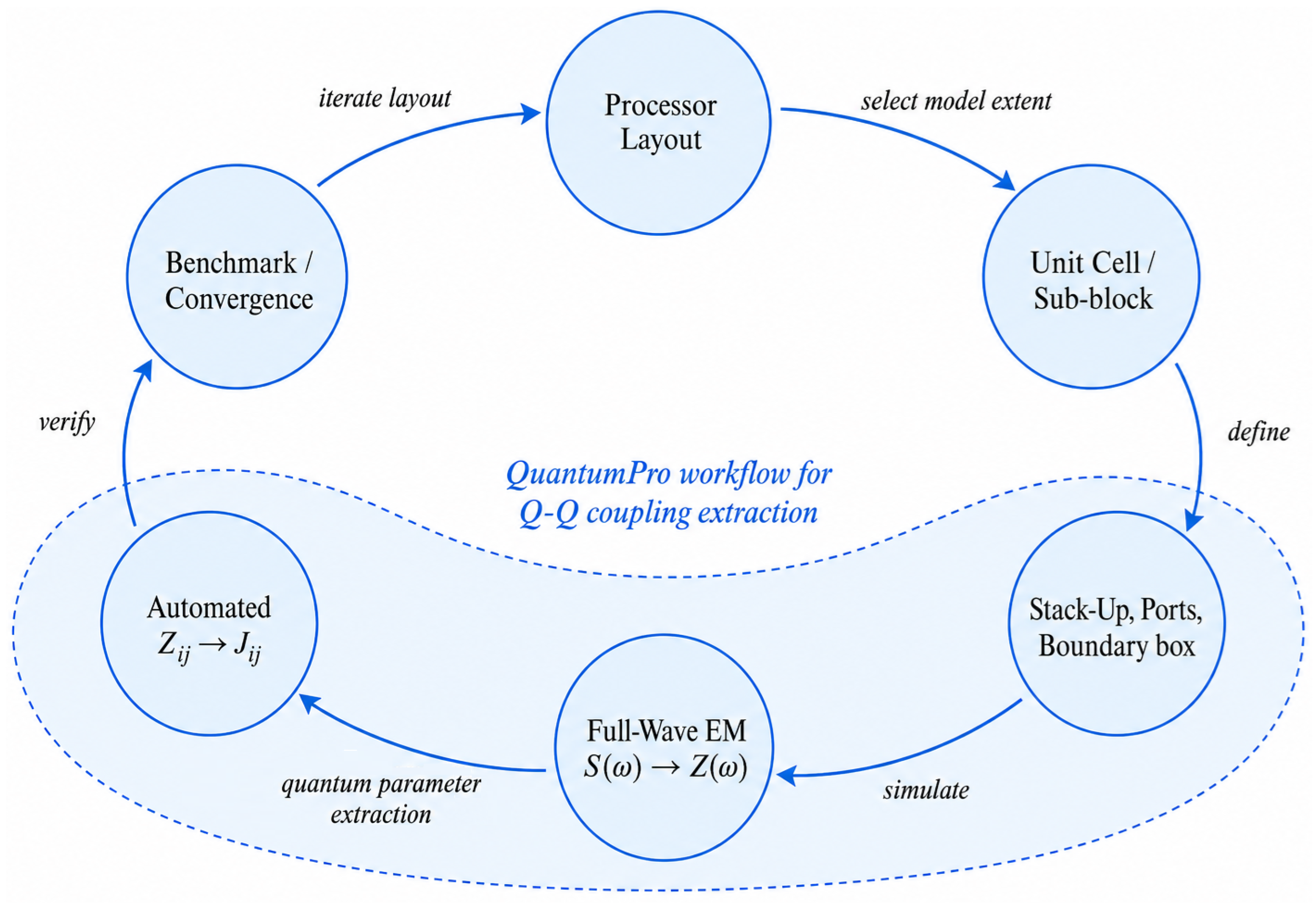
The workflow maps a processor layout to pairwise exchange couplings, as summarized in Figure 1. After the layout and electromagnetic stack-up are defined, QuantumPro performs the full-wave multiport analysis, automatically identifies the qubit ports, and extracts the pairwise exchange couplings. The port treatment, network conversion, and meshing strategy are described in the following subsections.

Figure 1. Overview of the full-wave workflow in Keysight Advanced Design System (ADS) and QuantumPro for pairwise exchange-coupling extraction in weakly anharmonic superconducting circuits operating in the dispersive regime, from layout construction and EM simulation to automated impedance-to-J evaluation and convergence checks.

2.3. Benchmark Device and Reduced EM Models

The IBM Q 16 Rueschlikon processor reported by Solgun et al. [14] is used as the benchmark because published imagery, qubit parameters, and nearest-neighbor coupling values are available for comparison. The processor geometry was reconstructed from the published optical micrograph and scale bar and therefore represents a geometry-constrained reconstruction rather than an exact reproduction of the fabrication layout.

Only nearest-neighbor couplings are considered in the benchmark because they correspond to the dominant coupling pathways intentionally engineered into the processor architecture and because published reference values are available for these interactions. The 16Q coupling-network model has also been used to verify that non-nearest neighbor couplings remain small; the detailed check is reported in Appendix A.

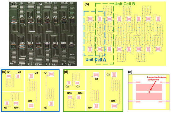
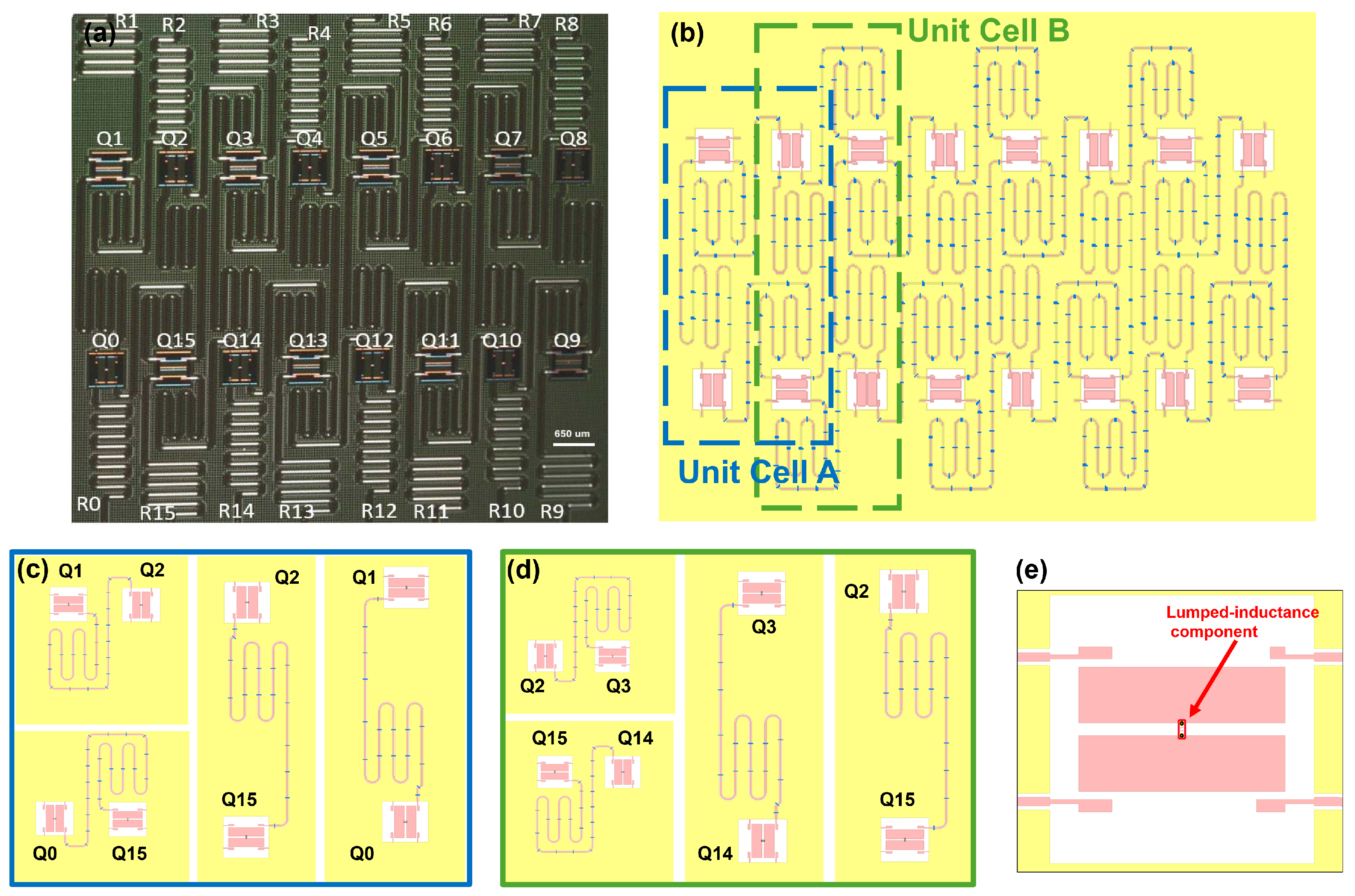
The model-reduction study starts from the 4Q unit cells because they match the model extent used by Solgun et al. [14] for the published full-wave coupling benchmark, denoted here as $J^S$. Figure 2a shows the published processor micrograph, while Figure 2b shows the reconstructed coupling geometry. Following the unit-cell definitions of Solgun et al. [14], Unit Cell A and Unit Cell B are reconstructed and translated across the processor to form four A-cell variants (A1–A4) and three B-cell variants (B1–B3). Each 4Q cell contains four nearest-neighbor coupling pairs, giving $4\times 4+3\times 4=28$ pair–cell instances for comparison with the published $J^S$ values. These 28 instances correspond to 22 unique physical nearest-neighbor links because six interior vertical links belong to both an A-cell and a B-cell and are therefore evaluated in both local electromagnetic environments.

Figure 2. Layout reconstruction and EM-model decomposition used for the coupling analysis. (a) Published optical micrograph of the IBM Q 16 Rueschlikon processor reported in Ref. [14], reproduced with permission from IEEE. (b) Reconstructed qubit-and-coupling geometry illustrating representative Unit Cell A and Unit Cell B regions. (c) Representative pair-specific 2Q reductions of Unit Cell A. (d) Representative pair-specific 2Q reductions of Unit Cell B. (e) Transmon-pocket definition in ADS showing the lumped effective inductance $L_i$ and the predefined connection points used for the qubit-port representation.

The same qubit and coupling-bus geometries are then assembled into the 16Q coupling-network model shown in Figure 2b. Readout resonators visible in the original micrograph are omitted from all three model extents so that the 16Q, 4Q, and 2Q comparisons contain the same types of coupling structures. The 16Q model is therefore the largest coupling-network model used here, not a fabrication-complete copy of the original chip.

Each 4Q cell is also reduced to pair-specific 2Q sub-blocks. Representative Unit-A and Unit-B reductions are shown in Figure 2c,d. The analysis is repeated for all horizontal and vertical nearest-neighbor pairs. The six interior vertical links shared by an A-cell and a B-cell are evaluated in both contexts because the surrounding retained geometry differs, whereas the horizontal links in the A- and B-cell sets correspond to distinct physical connections.

The resulting model set supports two comparisons: an external benchmark of the reconstructed 4Q cells against the published $J^S$ values and a same-reconstruction 16Q–4Q–2Q comparison that quantifies sensitivity to the retained EM domain. Geometry, material stack-up, junction locations, ports, and extraction settings are otherwise held fixed.

2.4. Port Definition and Electromagnetic Stack-Up

The qubit geometry is implemented using the built-in Quantum Artwork transmon-pocket component in ADS. Each Josephson junction is represented by a lumped inductance $L_i$ corresponding to its effective linearized value. The lumped-inductance component and its associated observation-port terminals are connected to the two transmon islands through predefined connection points located at the centers of the opposing island edges, as shown in Figure 2e. These connection points are used consistently throughout the reconstructed layout. For a given physical pair, the transmon geometry and connection-point locations are unchanged among the 2Q, 4Q, and 16Q models, so port placement is not an additional variable in the model-reduction comparison. Nevertheless, mesh sensitivity near the qubit connection points is examined in Section 3.

QuantumPro automatically detects the qubit elements and uses their observation ports for both qubit-frequency and transfer-impedance extraction. The specified effective inductance $L_i$ is included when analyzing the resonant qubit frequency $f_i$, whereas it is excluded when extracting the passive multiport response used to obtain $\mathbf{Z}\left(\omega \right)$. The transfer impedance is then evaluated at the extracted qubit frequencies and combined with $L_i$ and $L_j$ in Equation (1) to calculate $J_{ij}$. The observation-port orientation is kept consistent throughout the extraction; reversing a port changes the sign of the corresponding transfer impedance but does not affect the reported coupling magnitudes $\left|J_{ij}\right|$.

The simulation stack-up uses a 750 $\mathsf{\mu }$m silicon substrate with relative permittivity ${\epsilon }_r=11.5$, surrounded by air regions. The 200 nm conductor layer contains the qubit metallization, ground structures, inductive features, and keep-out regions. An upper conductor layer represents airbridges separated from the device layer by an 8 $\mathsf{\mu }$m air gap. These parameters define a consistent surrogate stack-up; they are not intended to reproduce the undocumented details of the original IBM fabrication process.

2.5. Full-Wave Simulation, Mesh Strategy, and Network Conversion

Full-wave EM simulations are performed in QuantumPro using a method-of-moments (MoM) solver that is well suited to the predominantly planar structures considered here. For each 2Q, 4Q, or 16Q model, the multiport scattering matrix $\mathbf{S}\left(\omega \right)$ is computed over the frequency range containing the relevant resonances. An adaptive frequency sweep is used, which concentrates additional frequency samples in regions of strong S-parameter variation, including resonant features, rather than using uniformly spaced samples across the entire band.

The scattering response is converted to the impedance matrix $\mathbf{Z}\left(\omega \right)$ using the standard multiport transformation

$$\mathbf{Z}\left(\omega \right)={\mathbf{Z}}_0^{1/2}\left[\mathbf{I}+\mathbf{S}\left(\omega \right)\right]{\left[\mathbf{I}-\mathbf{S}\left(\omega \right)\right]}^{-1}{\mathbf{Z}}_0^{1/2},$$

(2)

where $\mathbf{I}$ is the identity matrix and ${\mathbf{Z}}_0$ contains the port reference impedances. All qubit ports use the same 50-$\mathsf{\Omega }$ reference, so ${\mathbf{Z}}_0=50\mathsf{\Omega }\mathbf{I}$ in the simulations reported here. The 50-$\mathsf{\Omega }$ reference is part of the network representation rather than a physical termination imposed on the open-circuit transfer impedance.

The mesh is refined most strongly on the port-connected transmon islands and the coupling/resonator structures that influence the transfer impedance. The same selected mesh setting is used for the 2Q, 4Q, and 16Q comparisons so that model-extent effects are not mixed with different discretizations.

2.6. Benchmark References and Comparison Metrics

Reference data are taken from Solgun et al. [14]. In addition to the simulated couplings $J^S$, the couplings inferred from experimental $ZZ$ measurements are denoted $J^M$. The 4Q-to-$J^S$ comparison is the primary external benchmark, with $J^M$ retained as a secondary experimental reference. The six vertical links shared by neighboring A and B cells are evaluated separately in each cell context. For those pairs, the $J^S$, 4Q, and 2Q results therefore retain two corresponding cell-specific values because the surrounding retained geometry differs. The aggregate statistics over the 28 instances treat these as distinct pair–cell instances, matching the unit-cell-specific benchmark; when a single value per physical link is required for the 16Q comparison, the convention is stated explicitly.

For the comparison between two quantities, the signed percentage change is defined as

$${\delta }^{A\leftarrow B}=100\times {\displaystyle \frac{J_A-J_B}{J_B}}\%.$$

(3)

For each aggregate comparison, the absolute percentage differences $\left|\delta \right|$ are averaged over all entries in the corresponding comparison set. For comparisons against the published reference values, this quantity is reported as the mean absolute percentage error (MAPE).

3. Results

3.1. Mesh Convergence and Numerical Checks

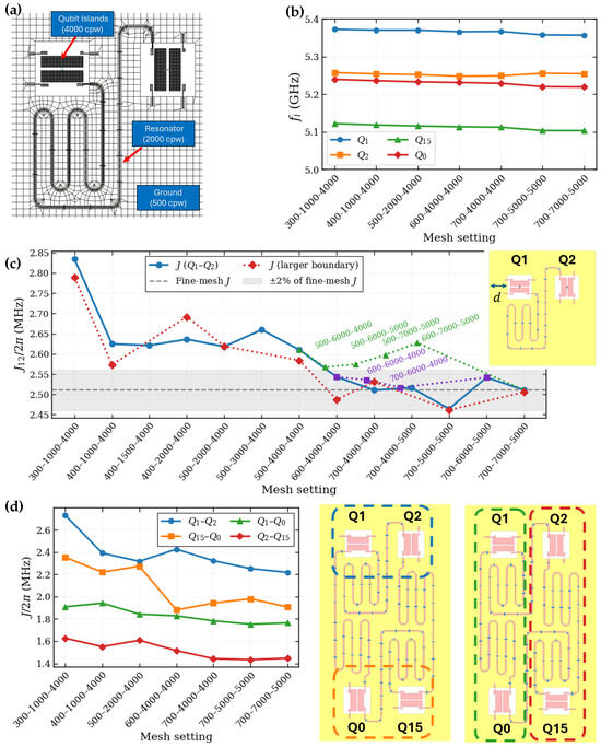
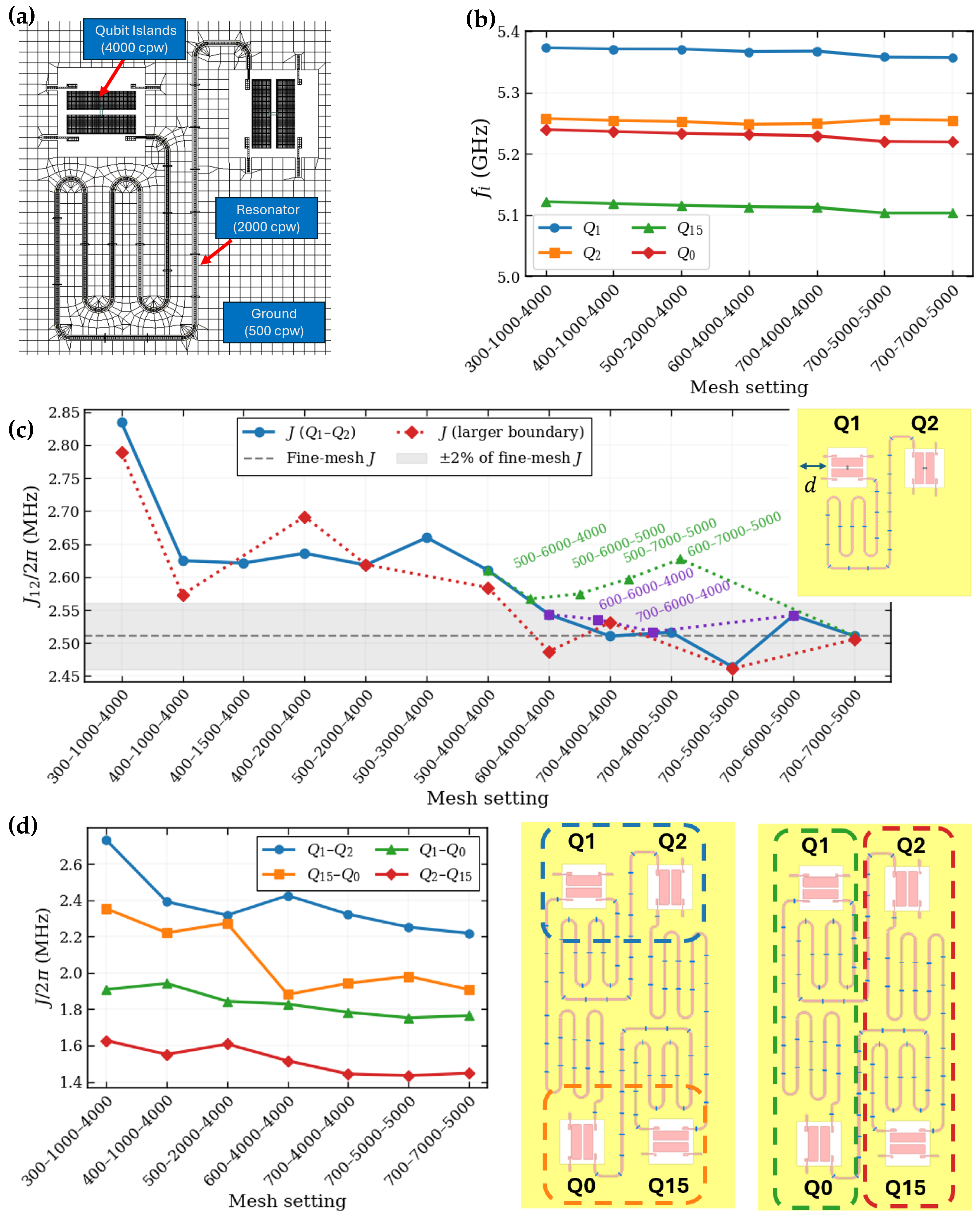
A mesh setting is written as G–C–P in cells per wavelength (cpw), where G, C, and P are the local mesh-density controls on the ground plane, coupling/resonator structures, and port-connected qubit islands, respectively, as shown in the illustrative example in Figure 3a. Larger cpw values correspond to finer local discretizations. This nonuniform mesh allows strong local refinement without applying the same density to the full ground plane.

Figure 3. Mesh labels use G–C–P in cpw for the ground plane, coupling/resonator structures, and port-connected qubit islands, respectively. (a) Nonuniform mesh of the pair-specific 2Q $Q_1$–$Q_2$ model at 500–2000–4000; this setting is shown to make the local mesh structure visible and is not the selected mesh setting. (b) Qubit-frequency convergence for the representative 4Q Unit-A1 model ($Q_1$, $Q_2$, $Q_{15}$, and $Q_0$). (c) Coupling convergence of the pair-specific 2Q $Q_1$–$Q_2$ model along multiple mesh-refinement paths and for nominal $d=400\mathsf{\mu }\mathrm{m}$ and enlarged $d=900\mathsf{\mu }\mathrm{m}$ domain clearances; the dashed line denotes the fine-mesh J reference obtained at 700–7000–5000, which was taken as the terminal point of the refinement study after the tested refinement branches had stabilized within approximately $\pm 2\%$; the shaded region denotes this $\pm 2\%$ convergence band. (d) Pairwise nearest-neighbor coupling convergence within the 4Q Unit-A1 configuration for $Q_1$–$Q_2$, $Q_{15}$–$Q_0$, $Q_1$–$Q_0$, and $Q_2$–$Q_{15}$, providing a 4Q confirmation of the mesh regime identified from the detailed 2Q study.

The convergence study in Figure 3b for a representative 4Q Unit-A1 model shows that qubit frequencies are relatively insensitive to mesh refinement, in contrast to the extracted coupling, shown in Figure 3c. In these calculations, J is more mesh-sensitive because it is obtained from the off-diagonal transfer impedance between the qubit observation ports and therefore depends on the local current distribution and discretization on the port-connected islands and coupling structures. This sensitivity motivates the stronger local refinement of the P regions and the use of $\left|J\right|$ itself as the convergence quantity.

Because the mesh sweep varies the three controls G, C, and P independently, there is no unique scalar mesh parameter that can order all tested combinations. The x-axis in Figure 3c therefore shows a representative refinement path in which the mesh controls are progressively increased, while the additional labeled points indicate alternative refinement branches obtained by varying one or more of the three controls differently. For the representative 2Q $Q_1$–$Q_2$ model shown in Figure 3c, different mesh-refinement paths approach the same coupling region. Once the finer tested settings along the different refinement branches remained within approximately $\pm 2\%$ of a common coupling value, the refinement study was considered sufficiently converged, and the 700–7000–5000 result was used as the fine-mesh J reference. Increasing the reduced-domain clearance from 400 $\mathsf{\mu }$m to 900 $\mathsf{\mu }$m slightly changes the refinement trajectory, but both cases ultimately converge to similar coupling values. A separate vertical $Q_1$–$Q_0$ test exhibits a similar convergence trend.

The detailed 2Q refinement study in Figure 3c is used to identify 700–4000–4000 as a practical mesh setting, with subsequent refinement resulting in diminishing coupling changes. The 4Q Unit-A1 results in Figure 3d then confirm that this setting remains in a weakly mesh-sensitive regime at the unit-cell level. In particular, refinement from 700–4000–4000 to 700–5000–5000 changes the 4Q couplings by 2.47% on average, with corresponding mean changes of 1.52% for the 2Q models and 1.80% for the independent 16Q refinement check. The selected 700–4000–4000 setting is then held fixed for all subsequent model-extent comparisons so that changes in extracted coupling are not mixed with changes in numerical discretization.

The adaptive frequency sweep is also checked against a conventional linear sweep on the 16Q coupling-network model. In the tested comparison, the linear sweep reproduces the adaptive-sweep coupling magnitudes within 2% but requires substantially longer simulation time. The adaptive sweep is therefore used for the final calculations.

3.2. External Benchmark Against Solgun et al.

Across all 28 pair–cell instances at 700–4000–4000, the 4Q MAPE relative to the corresponding published $J^S$ values is 3.70%, with an 8.69% worst case. Twenty instances are within 5%, and all 28 are within 10%. This agreement supports the reconstructed 4Q EM models together with the automated impedance-to-J extraction. Table 1 summarizes the benchmark; complete values are listed in Appendix A.

Table 1. Summary of the 4Q benchmark against Solgun et al. [14] at 700–4000–4000. Frequency errors use the reported qubit frequencies; coupling statistics are evaluated over the 28 pair–cell instances using the corresponding simulated $J^S$ values.

Quantity	MAPE (%)	Worst-Case Error (%)	Within 10%
Qubit frequency $f_i$	0.55	1.49	16/16
Coupling $\left|J\right|/2\pi$	3.70	8.69	28/28

The 16Q model provides a secondary external comparison. Because the 16Q model yields one coupling value per physical nearest-neighbor link, the six vertical links that appear in both Unit-A and Unit-B cells require the selection of a single $J^S$ reference when computing an aggregate error over the 22 unique physical links. Using the Unit-A values for these shared links gives a MAPE of 4.13% relative to $J^S$ and 6.94% relative to $J^M$. Using the Unit-B values instead changes the MAPE only slightly, to 3.98%. Table A2 retains both Unit-A and Unit-B values and reports the common 16Q value for each shared physical link.

3.3. Model-Reduction Accuracy: 16Q–4Q–2Q

The 16Q coupling-network calculation provides the largest-model reference within the same reconstruction. Reducing 16Q to the corresponding 4Q cells changes the couplings across the 28 pair–cell instances by 3.62% on average, with a 12.59% worst case; 27 of 28 remain within 10%.

Reducing 4Q further to 2Q changes the couplings by 6.17% on average, with a 12.07% worst case. The direct 2Q-to-16Q difference is 5.90% on average, but this endpoint value can hide cancellation between the two reduction steps. Table 2 summarizes the aggregate changes; the signed pairwise changes and a representative cancellation example are given in Appendix A.

Table 2. Summary of the same-reconstruction model-reduction comparison at 700–4000–4000 over the 28 pair–cell instances. Values are mean absolute relative changes in the extracted exchange coupling, using the second model named in each comparison as the denominator according to Equation (3).

Comparison	Mean Absolute Difference (%)	Worst-Case Difference (%)	Within 10%
4Q vs. 16Q	3.62	12.59	27/28
2Q vs. 4Q	6.17	12.07	25/28
2Q vs. 16Q	5.90	18.06	24/28

The qubit frequencies are less sensitive to model extent than the couplings. The 4Q frequencies agree with values reported by Solgun et al. [14] with a 0.55% MAPE and 1.49% worst-case error. Within the same reconstruction, the mean differences are 0.14% for 4Q–16Q, 0.19% for 2Q–4Q, and 0.32% for 2Q–16Q; all corresponding worst cases are below 0.5%. Complete frequency values are listed in Appendix A.

3.4. Computational Cost

Table 3 compares simulation time and peak memory for representative single solves of the 2Q, 4Q, and 16Q models. For these representative test cases, the 16Q calculation takes approximately 7.2 times as long as 4Q and requires 5.7 times the peak memory. Relative to 2Q, the representative 16Q solve takes approximately 36 times as long and requires about 19 times the peak memory. All representative cost measurements were obtained on a workstation equipped with two Intel Xeon Gold 6136 processors at 3.00 GHz and 768 GB of RAM.

Table 3. Computational cost of representative single 2Q, 4Q, and 16Q electromagnetic solves at the selected mesh setting. Reported times are wall-clock times for the individual simulations.

Model	Simulation Time	Peak RAM
2Q	6.98 min	3.95 GB
4Q	35.5 min	13.0 GB
16Q	4.24 h	73.9 GB

4. Discussion

4.1. Interpretation and Practical Role of the Model Extents

The results indicate that the appropriate EM model extent depends on the intended task. The 4Q unit cells provide the strongest accuracy–cost compromise for quantitative local coupling prediction in the reconstructed topology: they retain substantially more of the larger-model coupling environment than the pair-specific reductions while remaining much less computationally demanding than 16Q. This provides a complementary numerical-analysis perspective on the four-qubit unit-cell treatment of Solgun et al. [14], with the availability of the 16Q full-wave coupling-network model allowing the reduced-domain assumption itself to be tested quantitatively through controlled same-reconstruction comparisons across model extents.

The 2Q models can still be useful as inexpensive platforms for mesh-convergence screening and local sensitivity studies as shown in the Results section. However, their absolute coupling values are more sensitive to the omitted surrounding EM environment and should therefore not be interpreted as accurate substitutes for the larger model extents.

The 16Q model provides the larger-context reference needed to quantify this model-extent dependence. The complete 16Q→4Q→2Q path is informative because successive reduction shifts can partially cancel, so close agreement between the 2Q and 16Q endpoints alone does not establish insensitivity to the omitted environment. Thus, the three model extents have complementary roles: 2Q for numerical convergence and local sensitivity screening, 4Q for quantitative local prediction and early-stage design iteration, and 16Q for larger-context and final verification.

4.2. Sources of Discrepancy and Limitations

The same-reconstruction comparison primarily isolates model-extent effects because geometry, stack-up, ports, qubit parameters, extraction settings, and mesh policy are held fixed. In contrast, the 4Q-to-$J^S$ comparison also contains uncertainty from image-based reconstruction, undocumented fabrication and material details, kinetic-inductance assumptions, and differences in numerical formulation and solver implementation. The present work uses surface-current-based MoM, whereas the benchmark full-wave calculations of Solgun et al. [14] used volumetric FEM. Differences in discretization and numerical formulation may therefore contribute to the remaining benchmark discrepancy. That discrepancy should be interpreted as end-to-end agreement between independently constructed EM models rather than as an error of the impedance relation itself.

A controlled sensitivity study of substrate permittivity, conductor properties, airbridge geometry, package/ground extent, and domain-boundary placement would be required to attribute the remaining discrepancy to specific physical or numerical mechanisms. Such an analysis is left for future work. More generally, the numerical error levels reported here should not be extrapolated without additional validation to different coupler topologies, stronger hybridization, tunable couplers, or dense multimode and package environments. A broader processor-level assessment would also need to consider residual $ZZ$ interaction, mode crowding, package modes, control and readout crosstalk, dissipation, and fabrication variability [15,22].

4.3. Reproducibility, Applicability, and Design Use

For reproducibility, the layout revision, stack-up, port map, qubit parameters, solver settings, S-parameter data, S-to-Z conversion, and Equation (1) evaluation should be recorded together. Keeping this chain consistent prevents sign, port-order, or reference-impedance errors from being mistaken for physical layout changes.

When the layout uses Quantum Artwork qubit definitions and the stack-up and solver settings are specified consistently, the automated extraction inherits the port map, and the pairwise $J_{ij}$ matrix can be recalculated directly after a full-wave analysis as the design changes. This supports coupling-aware layout iteration without manually remapping EM ports to physical qubits for each analysis.

5. Conclusions

We implemented and benchmarked an automated QuantumPro workflow for extracting pairwise superconducting qubit–qubit exchange couplings from layout-level full-wave multiport responses using the Solgun method [14]. Across 28 pair–cell instances, the reconstructed 4Q models reproduce the published $J^S$ values with a 3.70% MAPE. Within the same reconstruction, the 4Q models differ from the 16Q reference by 3.62% on average while providing substantial reductions in simulation time and peak memory usage, supporting their use for early-stage design iteration. The larger changes observed for the 2Q models support their use primarily for convergence and local sensitivity screening rather than quantitative coupling prediction.

The validated workflow combines automated exchange-coupling extraction within a commercial microwave EDA environment with a practical strategy for selecting the EM model extent of a superconducting processor layout according to the required accuracy and available computational resources. Future work can extend the present validation in several directions. A controlled sensitivity analysis of substrate permittivity, conductor properties, airbridge geometry, package/ground extent, and domain-boundary placement would help quantify the physical and numerical sources of the remaining discrepancy. The workflow can also be evaluated for other coupling topologies, including tunable couplers and more strongly hybridized or multimode environments, and extended beyond exchange coupling to additional interaction metrics such as residual $ZZ$ coupling. Such studies would further establish the range of model extents and simulation settings required for broader processor-level design applications.

References

- Devoret, M.H.; Schoelkopf, R.J. Superconducting circuits for quantum information: An outlook. Science 2013, 339, 1169–1174. [Google Scholar] [CrossRef] [Scilit] [PubMed]
- Wendin, G. Quantum information processing with superconducting circuits: A review. Rep. Prog. Phys. 2017, 80, 106001. [Google Scholar] [CrossRef] [Scilit] [PubMed]
- Kjaergaard, M.; Schwartz, M.E.; Braumüller, J.; Krantz, P.; Wang, J.I.-J.; Gustavsson, S.; Oliver, W.D. Superconducting qubits: Current state of play. Annu. Rev. Condens. Matter Phys. 2020, 11, 369–395. [Google Scholar] [CrossRef] [Scilit]
- Krantz, P.; Kjaergaard, M.; Yan, F.; Orlando, T.P.; Gustavsson, S.; Oliver, W.D. A quantum engineer’s guide to superconducting qubits. Appl. Phys. Rev. 2019, 6, 021318. [Google Scholar] [CrossRef] [Scilit]
- Krinner, S.; Kurpiers, P.; Royer, B.; Magnard, P.; Tsitsilin, I.; Besse, J.-C.; Remm, A.; Blais, A.; Wallraff, A. Demonstration of an all-microwave controlled-phase gate between far-detuned qubits. Phys. Rev. Appl. 2020, 14, 044039. [Google Scholar] [CrossRef] [Scilit]
- Chow, J.M.; Gambetta, J.M.; Cross, A.W.; Merkel, S.T.; Rigetti, C.; Steffen, M. Microwave-activated conditional-phase gate for superconducting qubits. New J. Phys. 2013, 15, 115012. [Google Scholar] [CrossRef] [Scilit]
- Paraoanu, G.S. Microwave-induced coupling of superconducting qubits. Phys. Rev. B 2006, 74, 140504. [Google Scholar] [CrossRef] [Scilit]
- Zhao, P.; Xu, P.; Lan, D.; Chu, J.; Tan, X.; Yu, H.; Yu, Y. High-contrast ZZ interaction using superconducting qubits with opposite-sign anharmonicity. Phys. Rev. Lett. 2020, 125, 200503. [Google Scholar] [CrossRef] [Scilit] [PubMed]
- Noguchi, A.; Osada, A.; Masuda, S.; Kono, S.; Heya, K.; Wolski, S.P.; Takahashi, H.; Sugiyama, T.; Lachance-Quirion, D.; Nakamura, Y. Fast parametric two-qubit gates with suppressed residual interaction using the second-order nonlinearity of a cubic transmon. Phys. Rev. A 2020, 102, 062408. [Google Scholar] [CrossRef] [Scilit]
- Sung, Y.; Ding, L.; Braumüller, J.; Vepsäläinen, A.; Kannan, B.; Kjaergaard, M.; Greene, A.; Samach, G.O.; McNally, C.; Kim, D.; et al. Realization of high-fidelity CZ and ZZ-free iSWAP gates with a tunable coupler. Phys. Rev. X 2021, 11, 021058. [Google Scholar] [CrossRef] [Scilit]
- Wei, K.X.; Magesan, E.; Lauer, I.; Srinivasan, S.; Bogorin, D.F.; Carnevale, S.; Keefe, G.A.; Kim, Y.; Klaus, D.; Landers, W.; et al. Hamiltonian engineering with multicolor drives for fast entangling gates and quantum crosstalk cancellation. Phys. Rev. Lett. 2022, 129, 060501. [Google Scholar] [CrossRef] [Scilit] [PubMed]
- Nigg, S.E.; Paik, H.; Vlastakis, B.; Kirchmair, G.; Shankar, S.; Frunzio, L.; Devoret, M.H.; Schoelkopf, R.J.; Girvin, S.M. Black-box superconducting circuit quantization. Phys. Rev. Lett. 2012, 108, 240502. [Google Scholar] [CrossRef] [Scilit] [PubMed]
- Minev, Z.K.; Leghtas, Z.; Mundhada, S.O.; Christakis, L.; Pop, I.M.; Devoret, M.H. Energy-participation quantization of Josephson circuits. npj Quantum Inf. 2021, 7, 131. [Google Scholar] [CrossRef] [Scilit]
- Solgun, F.; DiVincenzo, D.P.; Gambetta, J.M. Simple impedance response formulas for the dispersive interaction rates in the effective Hamiltonians of low anharmonicity superconducting qubits. IEEE Trans. Microw. Theory Tech. 2019, 67, 928–948. [Google Scholar] [CrossRef] [Scilit]
- Solgun, F.; Srinivasan, S. Direct calculation of ZZ interaction rates in multimode circuit quantum electrodynamics. Phys. Rev. Appl. 2022, 18, 044025. [Google Scholar] [CrossRef] [Scilit]
- Abdelrahman, M.I.; Choi, J.; Slater, D.; Parker, T.; Krantz, P.; Sohn, P.; Hassan, M.A.; Mueth, C. Electromagnetic modeling and scripted quantum parameter extraction of 3D superconducting qubits using PathWave EMPro. In Proceedings of the 2023 IEEE International Conference on Quantum Computing and Engineering (QCE), Bellevue, WA, USA, 17–22 September 2023; pp. 352–353. [Google Scholar]
- Choi, J.; Abdelrahman, M.I.; Slater, D.; Parker, T.; Krantz, P.; Sohn, P.; Hassan, M.A.; Mueth, C. QuantumPro: An integrated workflow for the design of superconducting qubits using PathWave Advanced Design System (ADS). In Proceedings of the 2023 IEEE International Conference on Quantum Computing and Engineering (QCE), Bellevue, WA, USA, 17–22 September 2023; pp. 224–225. [Google Scholar]
- Shanto, S.; Kuo, A.; Miyamoto, C.; Zhang, H.; Maurya, V.; Vlachos, E.; Hecht, M.; Shum, C.W.; Levenson-Falk, E. SQuADDS: A validated design database and simulation workflow for superconducting qubit design. Quantum 2024, 8, 1465. [Google Scholar] [CrossRef] [Scilit]
- Sommers, D.; Degnan, Z.; Gautam, D.; Chen, Y.-H.; Chiu, C.-C.; Fedorov, A.; Pakkiam, P. Open-source highly parallel electromagnetic simulations for superconducting circuits. arXiv 2025, arXiv:2511.01220. [Google Scholar]
- Forati, E.; Langley, B.W.; Nersisyan, A.; Molavi, R. On the electromagnetic couplings in superconducting qubit circuits. IEEE Trans. Appl. Supercond. 2026, 36, 1700519. [Google Scholar] [CrossRef] [Scilit]
- Khan, G.; Roth, T.E. Field-based formalism for calculating multiqubit exchange-coupling rates for transmon qubits. Phys. Rev. Appl. 2024, 22, 064084. [Google Scholar] [CrossRef] [Scilit]
- Levenson-Falk, E.M.; Shanto, S.A. A review of design concerns in superconducting quantum circuits. Mater. Quantum Technol. 2025, 5, 022003. [Google Scholar] [CrossRef] [Scilit]
Disclaimer/Publisher’s Note: The statements, opinions and data contained in all publications are solely those of the individual author(s) and contributor(s) and not of MDPI and/or the editor(s). MDPI and/or the editor(s) disclaim responsibility for any injury to people or property resulting from any ideas, methods, instructions or products referred to in the content. |
© 2026 by the authors. Licensee MDPI, Basel, Switzerland. This article is an open access article distributed under the terms and conditions of the Creative Commons Attribution (CC BY) license.