


Abstract
Image stitching aims to construct wide field-of-view scenes from multiple narrow-FoV images, yet existing deep learning-based approaches may introduce substantial computational and parameter overhead, limiting their applicability in efficiency-sensitive scenarios. To address this issue, we propose a lightweight deep stitching framework that integrates multi-scale feature fusion with attention-enhanced matching. Specifically, a transformer-based channel attention (TCA) block improves the discriminative capability of fused features in low-texture regions and enhances global consistency. A coordinate-aware correlation module (CACM) combines correlation-based matching with position-sensitive coordinate attention to support registration under parallax, while GhostNet serves as the shared backbone. On UDIS-D, the complete model achieves a 25.19 dB peak signal-to-noise ratio (PSNR) and a structural similarity index (SSIM) of 0.833 under the overlap-region protocol, with a reported full-system complexity of 19.28 giga multiply-accumulate operations (GMACs) and 52.86 M parameters. These results demonstrate a favorable accuracy–efficiency trade-off under the stated GMAC, runtime, and memory protocol and the potential of the proposed framework for resource-conscious image stitching applications.
1. Introduction
Image stitching is a fundamental technique for constructing wide field-of-view (FoV) scenes from multiple narrow-FoV images. It supports applications including autonomous driving [1], medical imaging [2], and video surveillance [3]. Early approaches have relied on hand-crafted geometric features, beginning with the scale-invariant feature transform (SIFT) [4] for keypoint detection and matching. Later studies incorporated line segments [5,6], large-scale edges [7], depth maps [8], and semantic planar regions [9] to improve alignment and structure preservation. Nevertheless, low-texture or repetitive-pattern regions remain difficult, and increasingly complex geometric processing can limit efficiency-sensitive applications.
Deep learning provides an alternative in which feature extraction and geometric alignment can be learned jointly. Convolutional neural network (CNN)-based stitching frameworks [10,11,12,13,14,15,16,17] have improved alignment in several challenging settings, but their computational and parameter costs vary substantially. Balancing alignment quality with model complexity therefore remains an important design objective, particularly when an application has limited compute or memory budgets.
Parallax caused by depth variation or camera translation is another persistent challenge because a single homography cannot generally align all scene planes. Local or multi-grid warps [18,19,20,21,22] increase deformation flexibility, but they may depend on sufficiently reliable correspondences and can introduce additional computation or shape distortion. These trade-offs motivate a coarse-to-fine formulation that combines a global transformation with a regularized local warp.
To address these considerations, we develop a lightweight stitching framework that combines multi-scale feature fusion, channel reweighting, correlation-based matching, and coarse-to-fine geometric estimation. The transformer-based channel attention (TCA) block is placed after multi-scale concatenation to model interactions between global-average and global-maximum channel descriptors and to reweight the fused channels.
The coordinate-aware correlation module (CACM) constructs a normalized patch-correlation volume and applies coordinate attention [23] to retain directional spatial information before motion regression. This design is intended to provide position-aware matching cues without claiming that occlusion, illumination variation, or every large-parallax case is explicitly resolved.
GhostNet [24] is used as the shared feature backbone and depthwise separable convolutions [25] are used in the regression branches. The resulting architecture is designed to reduce computational and parameter costs while retaining the two-stage homography-plus-thin-plate-spline (TPS) alignment structure.
The experiments reported in this manuscript evaluate the method on UDIS-D using peak signal-to-noise ratio (PSNR) and structural similarity index (SSIM) under the current protocol. The reported results show competitive alignment metrics together with 19.28 giga multiply-accumulate operations (GMACs) and 52.86 M parameters under the stated full-pipeline counting protocol; they do not establish real-time operation or deployment performance on resource-constrained hardware.
The main contributions of this work are summarized as follows:
- (1)
- A TCA block is used for hierarchical multi-scale feature fusion and pooled-descriptor channel-dependency modeling.
- (2)
- A CACM combines normalized patch correlation with coordinate attention before homography and TPS control-point regression.
- (3)
- GhostNet and lightweight operations are used to balance alignment performance and model complexity under the current UDIS-D evaluation protocol.
2. Related Work
In this section, we briefly review traditional image stitching methods and deep image stitching methods.
2.1. Traditional Image Stitching
Traditional image stitching methods are based on manually designed features. Brown and Lowe [4] established their invariant-feature-based panoramic stitching method as a baseline framework, leveraging SIFT features and random sample consensus (RANSAC) for global homography estimation. Subsequent studies explored alternative feature descriptors (e.g., SURF [26], FAST [27], ORB [28]) to optimize keypoint detection and matching. However, global homography-based methods often introduced misalignment artifacts in non-planar scenes, prompting a shift toward local warping strategies.
Gao et al. [18] proposed the DHW algorithm, which separated foreground and background alignment using distinct homographies, combined with seam blending for seamless stitching. Lin et al. [19] further advanced this concept with SVA stitching to mitigate transition boundary artifacts. Zaragoza et al. [20] introduced the APAP algorithm, partitioning images into grids for localized homography estimation. While APAP improved alignment flexibility, it suffered from projection distortion and poor performance in feature-sparse regions. To address these limitations, APAP+CI [29] introduced adaptive correspondence insertion to improve alignment in feature-sparse regions.
To balance alignment precision and shape preservation, hybrid deformation models emerged. Chang et al. [30] proposed SPHP warps, blending projective and similarity transformations to suppress perspective distortion in non-overlapping regions. Lin et al. [31] introduced AANAP stitching, combining local homographies with global similarity constraints. Chen et al. [32] strengthened this paradigm with the GSP algorithm, enforcing similarity transformations through optimized sparse systems to minimize structural distortion.
Recent advancements have focused on geometric feature fusion for robust alignment. Xiang et al. [5] integrated line-guided constraints with global similarity to enhance low-texture alignment. Jia et al. [6] proposed line-point consistence stitching, leveraging coplanar subregions and collinear constraints for structure preservation. Du et al. [7] introduced GES-GSP warping, utilizing large-scale edge constraints and adaptive similarity transitions. Concurrently, depth-aware methods [8] exploited depth maps and epipolar geometry for parallax-tolerant stitching.
Despite progress, traditional methods face inherent limitations: Complex geometric constraints struggle in texture-deficient scenarios, while computational inefficiency hinders practicality.
2.2. Deep Image Stitching
Recent advances in deep learning have revolutionized image stitching by shifting from handcrafted geometric features to data-driven semantic feature learning.
DeTone et al. [10] introduced HomographyNet for direct corner-displacement regression, and Nguyen et al. [11] developed an unsupervised photometric formulation. Content-aware masking [12], UDIS and UDIS2 [13,22], coplanarity-aware adversarial learning [14], pixel-wise warping [15], implicit neural reconstruction [16], and attention-based homography estimation [17] subsequently broadened the design space. Recent work has further examined residual homography–TPS warps with boundary constraints [33], optical-flow-based alignment and hole-aware composition [34], local patch alignment integrated with seam cutting [35], and the domain-shift behavior of deep homography estimators [36]. Collectively, these studies show that alignment flexibility, composition quality, generalization, and computational cost must be considered separately rather than inferred from a single overlap metric.
2.3. Lightweight Feature Extraction and Attention
GhostNet [24], MobileNetV3-Large [37], and ShuffleNetV2 × 1.0 [38] represent different compact feature-extraction strategies. Their classifier-level efficiency does not directly determine end-to-end stitching speed, so the present comparison retains identical TCA, CACM, regression, geometry, loss, preprocessing, and evaluation components and changes only the backbone plus the minimum 1 × 1 channel adapters required by the downstream interface. Coordinate attention [23] is established prior art; CACM’s contribution is its application to the target-indexed global correlation representation rather than invention of the attention operator itself.
Recent work includes pixel-wise alignment [39], progressive alignment with interwoven composition [40], hierarchical grid-constrained fusion [41], structure-preserving bidirectional pixel warps [42], segmentation-guided multi-homography warping [43], and depth-based stitching [44]. These methods highlight that overlap alignment, shape preservation, seam quality, and generalization require separate evidence. Related preliminary work introduced attention-guided multi-scale fusion [45]; the present study develops this direction through the integrated GhostNet–TCA–CACM coarse-to-fine architecture and adds controlled component, backbone, efficiency, and failure analyses.
Although recent systems increase deformation flexibility or explicitly optimize composition quality, their alignment, reconstruction, and computational objectives are not interchangeable. The present study therefore addresses a narrower accuracy–complexity trade-off on UDIS-D through a lightweight backbone, pooled-descriptor channel attention, and coordinate-aware correlation. Accordingly, the conclusions are drawn within the scope of the UDIS-D benchmark, overlap-region reconstruction metrics, and computational characteristics measured under the stated evaluation protocol.
3. Methodology
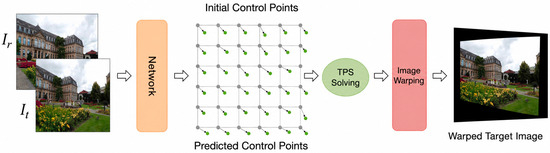
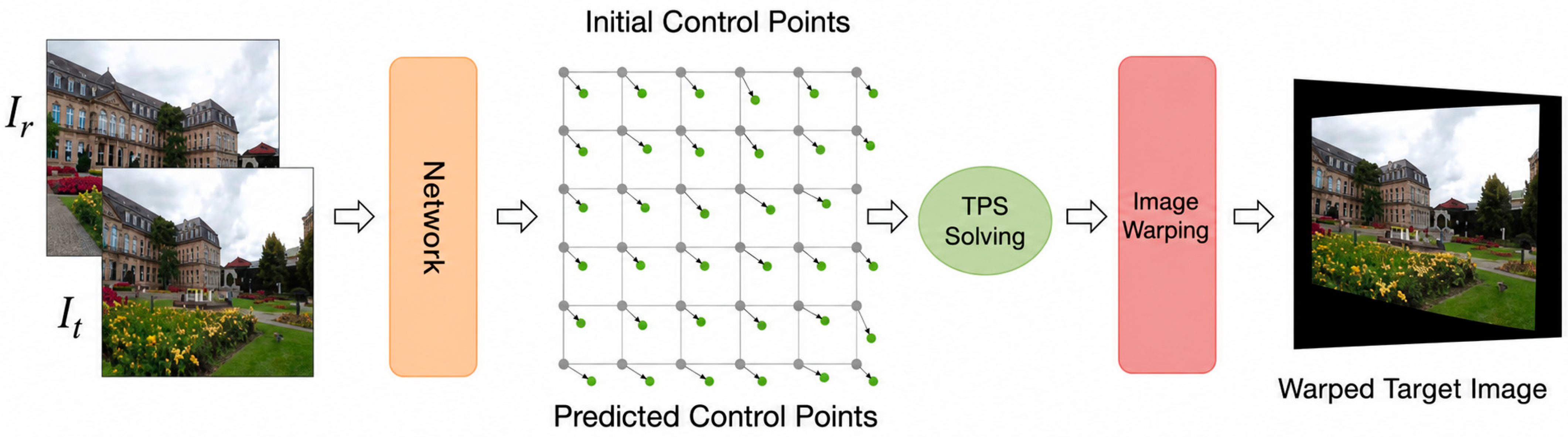
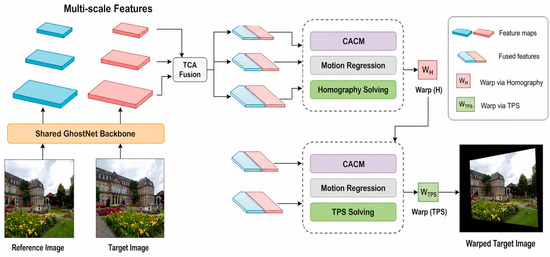
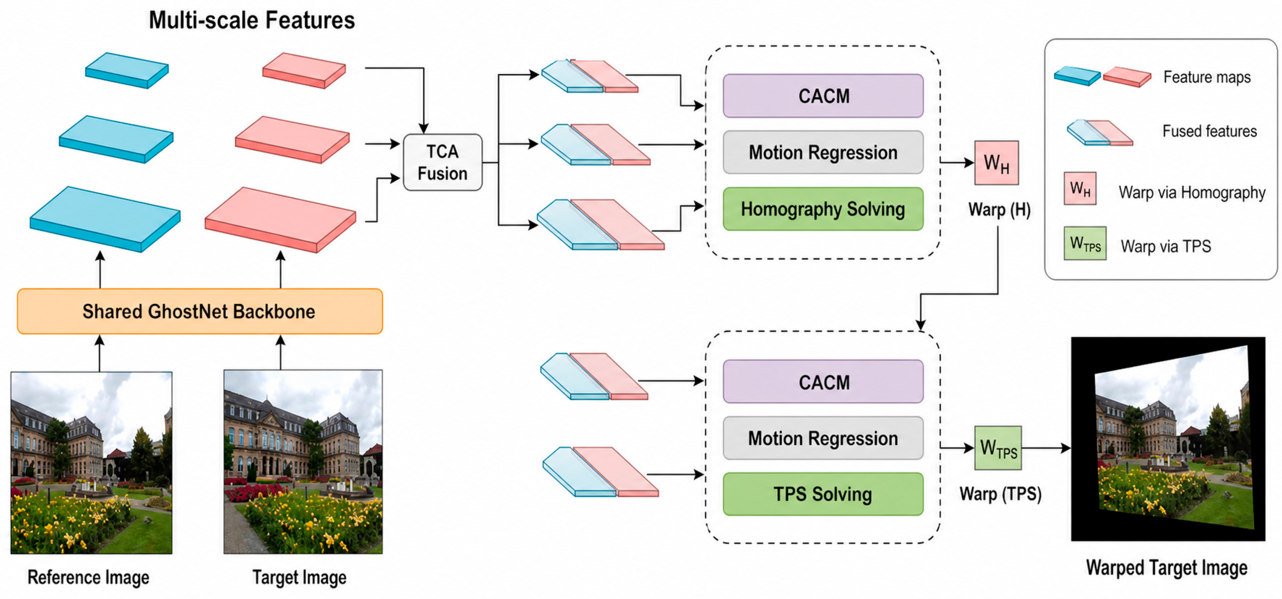
Figure 1 illustrates the local TPS transformation stage: the network predicts a control-point mesh relative to its initialized grid, and TPS solving transforms the input images. The complete registration framework is summarized in Figure 2. The network receives a reference image Ir and target image It, each with shape B × 3 × 512 × 512. A shared lightweight backbone extracts three feature scales. TCA-based fusion combines adjacent scales, and CACM constructs position-aware global correlation representations for two regression stages. The first stage predicts four two-dimensional corner offsets and solves a global homography. The second predicts offsets for a 13 × 13 control-point mesh initialized from the homography-warped regular grid. The resulting TPS warp is then used for target-image transformation, after which the reference and warped target are placed on a dynamic union canvas and average-fused in valid overlap. This ordering is coarse-to-fine; it does not guarantee seam-free composition or globally invertible TPS deformation.
Figure 1.
Local thin-plate spline (TPS) transformation: the network predicts dynamic control points, TPS solving relates them to the initialized control points, and the resulting mapping transforms the input images.
Figure 2.
Overall registration architecture: shared GhostNet reference and target branches feed contextual-correlation and motion-prediction stages for four-corner homography estimation and 169-point TPS-offset regression, followed by the corresponding warp operations.
3.1. Warp Parameterization
Let an arbitrary target-image location be p = (x, y)T. The regular image domain is divided into U = 12 by V = 12 cells, yielding N = (U + 1)(V + 1) = 169 grid vertices. Denote the regular grid by P0, the homography-initialized grid by P, the network-predicted local offsets by , and the final TPS control coordinates by . Equation (1) expresses the implemented update ; thus, P in this equation is the homography-initialized mesh rather than the unwarped regular grid .
By minimizing an energy function consisting of a data term and a distortion term [46], the TPS transformation can be parameterized as follows:
In Equation (2), f(p) ∈ R2 is the mapped coordinate, is the translation term, is the affine matrix, is the nonlinear weight associated with control point , and N = 169. The implementation uses the radial basis O(di) = di2 log(di2 + 10−6), where . For each batch item, the TPS linear system is assembled from the supplied normalized control-point pairs and its inverse is computed in double precision. The solve matrix is therefore batched rather than fixed, because the predicted source mesh varies across samples.
The global homography and local TPS are used sequentially. Four predicted corner offsets define the homography; the regular 13 × 13 grid is transformed by that homography; and the network then adds 169 local two-dimensional offsets before the TPS sampler is evaluated. The regularizer discourages excessive deformation but does not prove that every predicted mesh is invertible.
3.2. Network Structure
The overall registration architecture is shown in Figure 2. The reference and target branches share the GhostNet backbone; their multi-scale features feed contextual-correlation and motion-prediction stages that estimate a four-corner homography and 169 local TPS control-point offsets. The multi-scale representation allows larger-scale features to emphasize global structure and overall layout, whereas smaller-scale features retain texture and edge details. Their collaboration helps stabilize feature matching under large parallax and complex scene structure and provides a robust basis for estimating the two geometric transformations.
To reduce computational overhead while retaining multi-scale features, the network uses a shared GhostNet [24] backbone for the reference and target images. For a 512 × 512 input, the extracted features have 40 channels at ( scale), 112 channels at ( scale), and 960 channels at 16 × 16 ( scale). These tensors provide progressively coarser semantic and spatial information for the two fusion and regression stages.
Fusion proceeds hierarchically. The feature is first upsampled and concatenated with the feature; the result is channel-reweighted and compressed. That tensor is then upsampled and concatenated with the 64 × 64 feature, followed by a second TCA block and channel compression. This ordering preserves the actual coarse-to-fine data flow used by the implementation.
The first regression stage uses the 32 × 32 fused features to predict eight values representing four two-dimensional corner offsets. A direct linear transform constructs the global homography, which is used to coarsely warp the target feature. The second stage uses the fused features to predict 338 values, corresponding to two offsets for each of 169 TPS control points. The final control mesh is the homography-initialized regular mesh plus these local offsets, so the TPS refinement follows rather than replaces the global homography estimate.
3.2.1. Transformer-Based Channel Attention Module
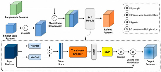
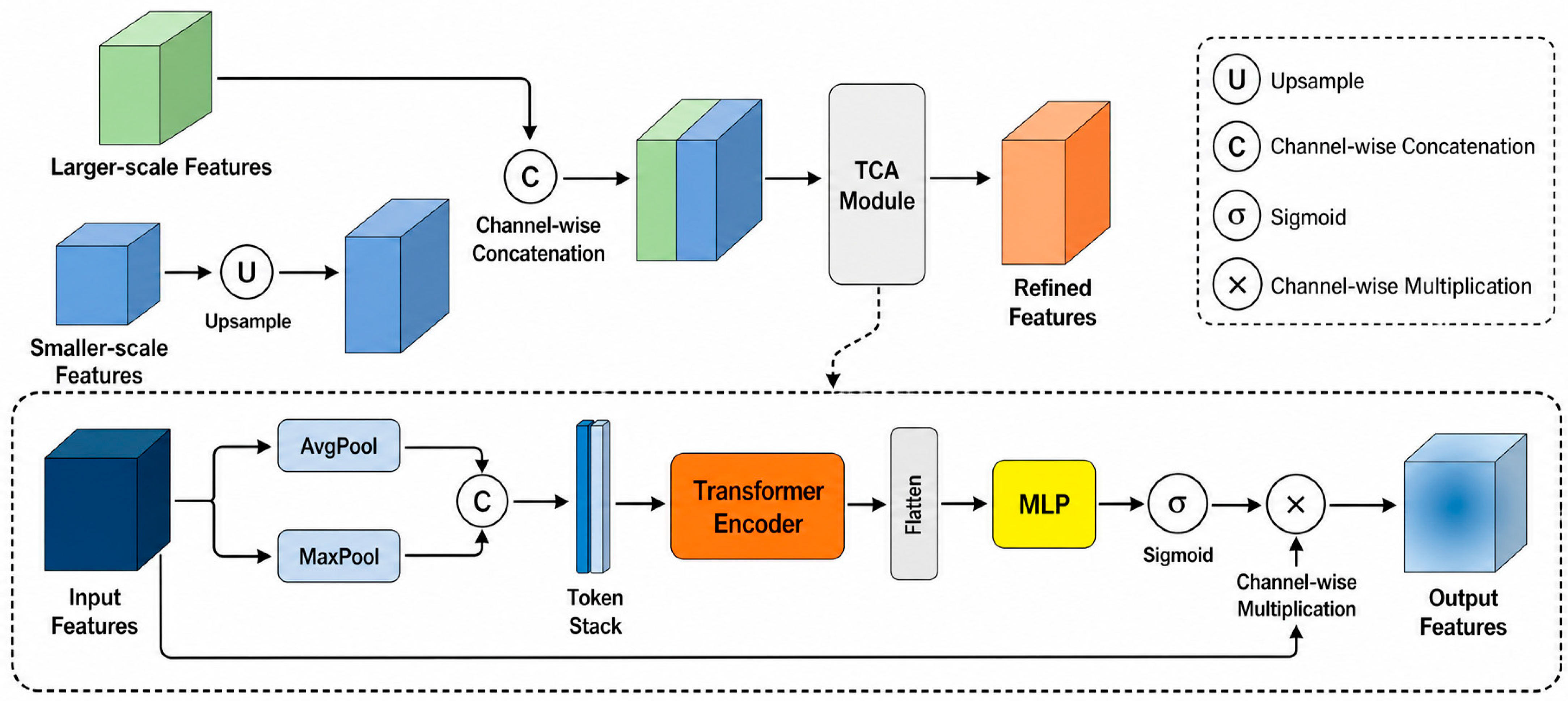
The transformer-based channel attention (TCA) block is applied after concatenating two spatially aligned feature maps (Figure 3). In the first fusion stage, the 960-channel 16 × 16 tensor is bilinearly upsampled with align_corners = True and concatenated with the 112-channel 32 × 32 tensor, producing 1072 channels; a convolution later compresses the reweighted result to 512 channels. In the second stage, that tensor is bilinearly upsampled and concatenated with the 40-channel 64 × 64 tensor, producing 552 channels before TCA and 256 channels after the subsequent 1 × 1 convolution.
Figure 3.
Multi-scale fusion with transformer-based channel attention (TCA): the upsampled smaller-scale feature is concatenated with the larger-scale feature; average- and max-pooled descriptors are processed by a transformer encoder and multilayer perceptron (MLP) to generate multiplicative channel weights.
Let the TCA input have shape B × C × H × W. Global average pooling (GAP) and global max pooling (GMP) each reduce the spatial dimensions, producing and , each with shape . GAP summarizes the average channel response, whereas GMP emphasizes strong activations. Their combination provides complementary channel descriptors for the subsequent attention operation. The descriptors are computed as follows:
where and are channel descriptors obtained from the same fused tensor .
The two descriptors are stacked as a two-token sequence. The intermediate tensor has shape and is transposed to 2 × B × C for the PyTorch transformer encoder:
The sequence is processed by one transformer encoder layer with embedding dimension , eight attention heads, the PyTorch-default feed-forward dimension of 2048, ReLU activation, dropout of 0.1, LayerNorm, and the encoder layer’s internal residual connections. The sequence length is two: the attention operates between the GAP and GMP descriptors and across their channel embeddings, not over all H × W spatial positions. Denoting the encoded sequence by ′ = T(), the tensor is returned to shape B × 2 × for channel-weight prediction.
The encoded two-token tensor is flattened to and passed through a channel MLP with dimensions . The hidden layer uses ReLU, and a sigmoid maps the output to channel weights:
where has shape and contains the sigmoid-normalized channel weights.
The weights are broadcast over H and W and multiplied elementwise with the original fused tensor, yielding . There is no additional outer residual term of the form ; residual connections occur only inside the standard transformer encoder layer. Combining average and maximum descriptors is intended to retain complementary global and salient responses, but this interpretation is not presented as an independently validated causal result.
3.2.2. Coordinate-Aware Correlation Module
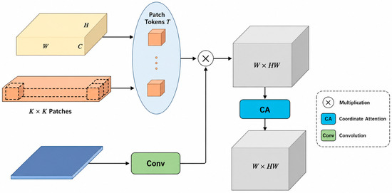
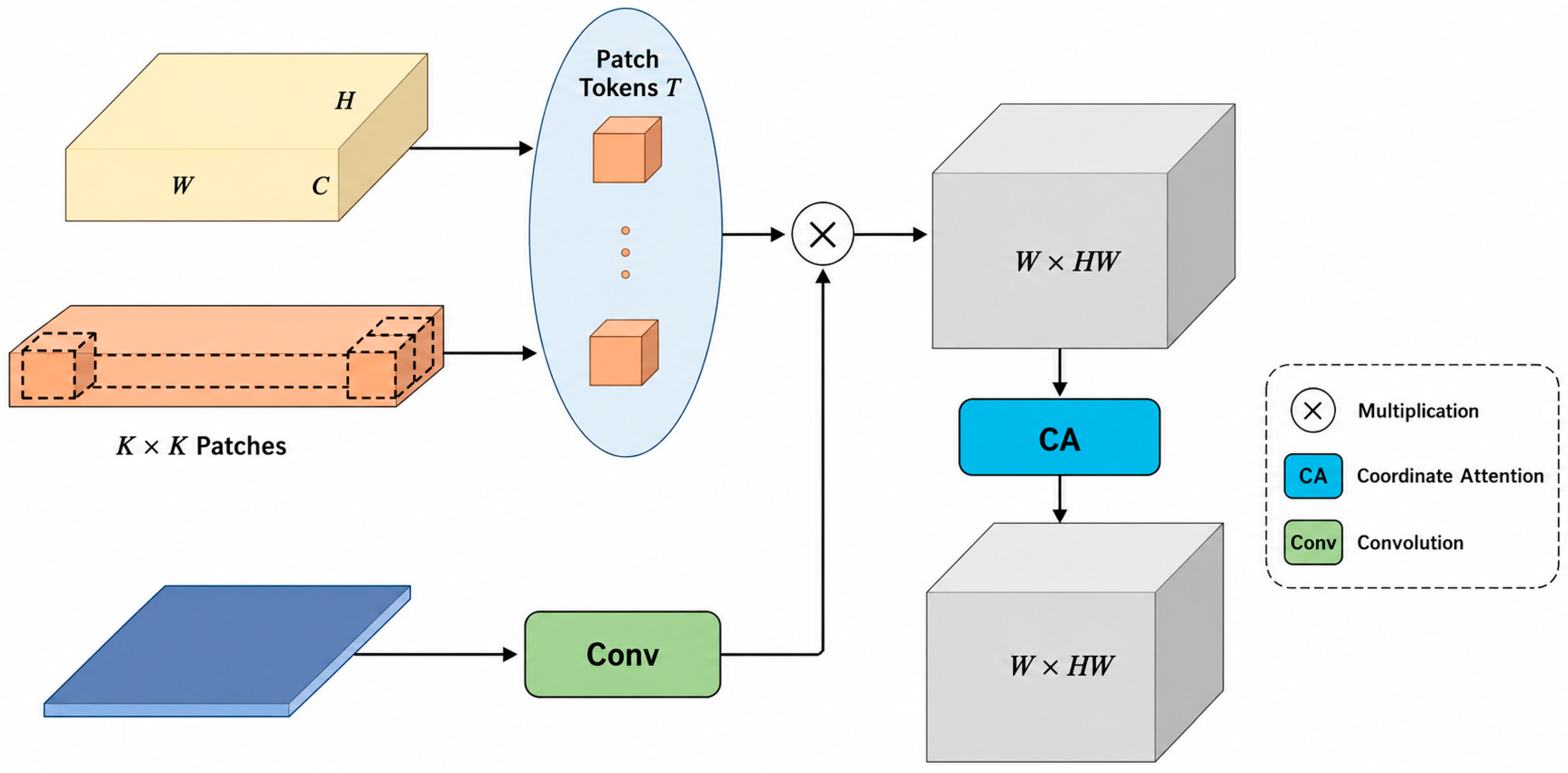
After multi-scale fusion, the registration stages must represent correspondences between the reference and target features. The coordinate-aware correlation module (CACM) combines normalized patch correlation with coordinate attention before motion regression (Figure 4). Its purpose is to provide position-sensitive matching features for geometric regression.
Figure 4.
Coordinate-aware correlation module (CACM) conceptual pipeline: target-patch correlations are evaluated exactly through pixel-wise all-pairs correlation and aligned 3 × 3 offset aggregation; coordinate attention reweights the resulting volume, and convolution produces the feature flow.
Conceptually, the target patches can be interpreted as dynamic filters applied to the reference feature map. CACM then treats target positions as correlation channels and reweights the correlation volume along the two reference spatial axes using coordinate attention.
Let and denote the reference and target features, each with shape . Both tensors are L2-normalized along the channel dimension. CACM extracts a K × K target patch at every spatial position with , stride 1, and zero padding 1, producing patches. In the conceptual formulation, these patches define B × HW dynamic filters of size C × applied to the corresponding reference feature map. For a target-centered patch , the correlation is summarized by Equation (6).
In Equation (6), indexes a target position, (x, y) indexes a reference position, indexes the 3 × 3 patch support, and c indexes the normalized feature channels.
Here, and denote feature vectors L2-normalized along the channel dimension at each spatial location. Out-of-range indices are treated as zero under the same padding convention as Equation (6). Under this dense nine-offset evaluation, the factorization requires MACs and scalar additions for , without changing the output correlation volume.
Equation (6) defines the patch-correlation operation conceptually. In the implementation, it is evaluated exactly by first computing pixel-wise all-pairs correlation between the normalized target and reference features, followed by aggregation over the nine aligned 3 × 3 offsets. This is an algebraic factorization rather than a low-rank or local-window approximation and produces the same correlation volume up to floating-point rounding.
Evaluating Equation (6) for every target and reference location yields a correlation volume with shape B × HW × . The second dimension enumerates all target centers, while the last two dimensions enumerate reference locations. Thus, the module uses local 3 × 3 descriptors but compares each target-centered descriptor over the full reference feature grid; it is not a displacement-only volume. No softmax normalization is applied to in the available implementation.
Coordinate attention [23] receives V with HW target positions treated as channels. Horizontal pooling averages the width axis and produces B × HW × H × 1, whereas vertical pooling averages the height axis and produces B × HW × 1 × W. After a shared projection, batch normalization, and ReLU, separate projections and sigmoids generate horizontal and vertical attention maps. Their broadcast product reweights V elementwise while retaining the reference coordinate axes.
The enhanced volume is passed through two , stride-1, padding-1 convolutions with channel dimensions and a ReLU between them, producing a feature flow of shape . At the stage, and this flow is used by the first regression branch to predict four corner offsets. At the 64 × 64 stage, HW = 4096 and the second branch predicts the 169 two-dimensional TPS control-point offsets.
3.3. Objective Function
Let Ir and It denote the reference and target images, respectively; W(X; θ) denote bilinear warping; and Mθ = W(J; θ) denote the warped validity field obtained from an all-one tensor J. The implemented color offsets and alignment loss are written explicitly in Equation (7a–d):
δH = [Σ W(It; H) − Σ(Ir ⊙ MH)]/ΣMH; δH−1 = [Σ W(Ir; H−1) − Σ(It ⊙ MH−1)]/ΣMH−1.
δTPS = [Σ W(It; TPS) − Σ(Ir ⊙ MTPS)]/ΣMTPS.
LH = ‖(Ir + δH) ⊙ MH − W(It; H)‖1 + ‖(It + δH−1) ⊙ MH−1 − W(Ir; H−1)‖1.
LTPS = ‖(Ir + δTPS) ⊙ MTPS − W(It; TPS)‖1; Lalignment = 3LH + LTPS.
Equation (7c) is bidirectional: it compares the target warped toward the reference and the reference warped by H−1 toward the target. The per-channel offsets in Equation (7a,b) are normalized by the sums of their corresponding warped validity fields. Equation (7d) gives the forward TPS term and the implemented 3:1 weighting between homography and TPS alignment. The validity fields exclude out-of-domain samples but do not explicitly model occlusion or non-corresponding regions. The per-channel offsets compensate for simple global photometric differences but do not account for spatially varying illumination changes.
The mesh-shape regularizer contains an intra-mesh term that limits excessive positive horizontal and vertical edge components and an inter-mesh term that penalizes angular changes between successive edges in regions marked as non-overlapping. These penalties discourage excessive local deformation but do not mathematically guarantee global injectivity or prevent every possible fold.
For a mesh with U = V = 12 cells, horizontal edges are differences between adjacent columns and vertical edges are differences between adjacent rows. The intra-mesh term applies ReLU to horizontal x components above and vertical y components above . With the implemented , both thresholds equal 85.33 pixels. The loss averages each component-wise penalty over its full horizontal or vertical edge tensor and sums the two means, as represented by Equation (8).
In Equation (8), i and j denote the horizontal and vertical unit directions, respectively, and σ(·) is ReLU. The available implementation constrains the corresponding signed edge components; it does not directly penalize every Euclidean edge length or every reversed edge.
The inter-mesh term measures 1 minus the cosine similarity of successive horizontal or vertical edge vectors. Neighboring angular errors are combined at the cell level and multiplied by a derived non-overlap indicator before averaging. Let and denote successive edges in the same direction; Equation (9) summarizes this angular penalty.
Here, denotes the set of candidate successive-edge pairs and is the derived indicator. In the code, the warped validity mask is averaged within each grid cell and a cell is marked 1 when that mean is below 0.9; despite the variable name overlap, this value functions as a non-overlap indicator. Transitions between differently marked cells are suppressed, and torch.mean averages the masked arrays including zero-valued inactive positions rather than normalizing only by the number of active pairs.
The two mesh terms therefore act as soft regularizers: the intra-mesh term discourages excessive directed expansion, and the inter-mesh term discourages bending across selected non-overlap cells. They reduce the objective assigned to these deformations but do not establish a strict no-folding guarantee:
The final overall objective function of the network can be expressed as follows:
Equation (11) defines the total objective as L = λLH + ω1LTPS + ω2(Lintra + Linter), where λ = 3, ω1 = 1, and ω2 = 10. Substitution gives the executed objective L = 3LH + LTPS + 10Lintra + 10Linter. These implemented values were fixed before the final evaluation; Section 4.7 subsequently reports a one-factor-at-a-time sensitivity analysis around this configuration. The results in the sensitivity analysis indicate that the model performance remains reasonably stable under moderate variations of these loss weights around the default configuration, supporting the robustness of the selected weighting scheme within the evaluated ranges.
4. Experiments and Results
4.1. Dataset and Evaluation Criterion
The experiments use the UDIS-D dataset [13], which contains image pairs derived from variable-motion videos. The UDIS-D training split used in this study contains 10,440 paired samples, and the test split contains 1106 pairs. Every image is resized once to 512 × 512 pixels by the dataset loader.
Dataset information summary.
| Field | Setting | Verification Source |
| Dataset | UDIS-D | Manuscript and local dataset directories |
| Source | Image pairs derived from variable-motion videos | UDIS/UDIS-D description [13] and manuscript |
| Training pairs | 10,440 | Count verified in training/input1 and training/input2 |
| Testing pairs | 1106 | Count matched in archived testing/input1 and testing/input2 |
| Input resolution | 512 × 512 pixels | dataset.py resize operation |
| Scene/source description | Variable-motion video frame pairs with real-scene overlap and parallax | Dataset documentation and [13] |
| Usage in this study | Unsupervised training and UDIS-D overlap-region evaluation | train.py, dataset.py, and manuscript |
Peak signal-to-noise ratio (PSNR) and the structural similarity index measure (SSIM) are used as overlap-region alignment metrics. They compare the reference image and the TPS-warped target over the warped valid-field region, as summarized in Equations (12) and (13). These metrics primarily assess overlap alignment and do not fully characterize seam quality or distortion in non-overlapping panorama regions.
PSNR and SSIM are calculated over the warped valid field of view and primarily quantify overlap-region alignment. For each separate metric, the 1106 test pairs are sorted into a top 300, a middle 506, or a bottom 300 score group, with the term ‘all’ denoting all 1106 pairs. These score partitions are not fixed scene difficulty labels based on parallax, texture, or semantics. Unless common image IDs are explicitly recorded, the groups must not be interpreted as identical difficulty subsets across methods.
4.2. Experiments Details
The network is implemented in PyTorch and trained on UDIS-D for a pre-specified 100 epochs using AdamW, with an initial learning rate of 1 × 10⁻⁴ and an exponential decay factor of 0.97 per epoch. Training uses a single NVIDIA GeForce RTX 4090 GPU, batch size 4, and 512 × 512 inputs. The checkpoint from the final training epoch (epoch 100) is used for evaluation according to the fixed training schedule and is not selected based on test-set performance.
Implementation configuration summary.
| Field | Setting | Verification Source |
| Framework | PyTorch | train.py |
| Python version | 3.8.5 | environment.yml |
| PyTorch version | 1.7.1 | environment.yml |
| GPU | Single NVIDIA GeForce RTX 4090 | Experimental setup record |
| Input resolution | 512 × 512 | dataset.py |
| Batch size | 4 | train.py default |
| Epochs | 100 | train.py default |
| Optimizer | AdamW, β = (0.9, 0.999), ε = 10−8 | train.py |
| Initial learning rate | 10−4 | train.py |
| Learning rate schedule | ExponentialLR, γ = 0.97 per epoch | train.py |
| Effective batch size | 4 (one process/GPU; no accumulation found) | train.py |
| Random seed | Random seed: not explicitly fixed in the implementation | No seed-setting call in the training script |
| Data augmentation | Random input-order swap; independent brightness and color multipliers sampled in [0.7, 1.3] | dataset.py |
| Training/testing split | 10,440 training pairs/1106 testing pairs | Local dataset directory counts |
| Checkpoint selection | Final checkpoint at epoch 100 | Run record and epoch100_model.pth |
| Mesh size U × V | 12 × 12 cells; 13 × 13 control points | grid_res.py and new_network.py |
| CACM patch size K | 3 × 3; stride 1; zero padding 1 | new_network.py |
| Transformer layers | 1 | new_network.py |
| Attention heads | 8 | new_network.py |
| Transformer feed-forward dimension | 2048 | PyTorch 1.7.1 default used by new_network.py |
| TCA channel MLP | 2C → C/8 → C | new_network.py |
All controlled experiments use the same UDIS-D split, preprocessing, 100-epoch training schedule, and evaluation code. The primary configuration—including the 12 × 12 mesh, 3 × 3 CACM patch, one transformer layer with eight attention heads, and loss weights (λ = 3, ω1 = 1, and ω2 = 10)—was fixed before the final test-set evaluation. Following the fixed training schedule, the checkpoint from epoch 100 is used for final evaluation. The 1106-pair test set is used for result reporting rather than for architecture, hyperparameter, or checkpoint selection. Section 4.7 provides a supplementary one-factor-at-a-time sensitivity analysis around the fixed loss-weight configuration.
Rationale for architectural hyperparameters. All architectural configurations were determined based on preliminary experiments on a held-out subset of the training split and established engineering conventions, with no access to the 1106-pair test set at any stage.
12 × 12 control mesh. We evaluated 8 × 8, 12 × 12, and 16 × 16 mesh configurations during preliminary training. The 8 × 8 mesh lacked sufficient deformation flexibility for parallax-rich scenes, while the 16 × 16 mesh sharply increased regression dimensionality and caused overfitting to local texture noise. The 12 × 12 mesh (169 control points) achieves the best trade-off between alignment capacity and computational stability, consistent with common settings in TPS-based image stitching literature.
3 × 3 CACM patch size. A 3 × 3 local support is a standard receptive field for dense feature matching. A 1 × 1 patch lacks spatial context and degrades matching robustness. Increasing the patch to 5 × 5 does not change the dimensions of the output correlation volume, which are determined by the target and reference feature-map sizes; it instead increases the aligned-offset aggregation from 9 to 25 terms per correlation entry, thereby increasing computation and memory traffic. The 3 × 3 setting balances matching discriminability and efficiency.
Single Transformer layer in TCA. The TCA module operates on only two pooled channel tokens (GAP and GMP). Adding more encoder layers did not yield measurable accuracy gains in preliminary experiments and increased overfitting risk. One layer is sufficient to model the interaction between the two channel descriptors while maintaining an extremely light weight.
Eight attention heads. The channel dimensions at both fusion stages (1072 and 552) are divisible by 8, making eight heads compatible with the standard PyTorch multi-head attention implementation. Preliminary tests with four heads showed no consistent accuracy improvement. A 16-head configuration was not evaluated because the 552-dimensional second-stage embedding is not divisible by 16 under the standard implementation. We therefore retained eight heads as the standard configuration.
None of these hyperparameters were tuned or selected based on test-set performance; the test partition is used exclusively for final result reporting.
4.3. Comparative Experiments
Table 1 presents the quantitative comparison with the learning-based methods UDIS, UDIS2, and AbHE under the UDIS-D overlap-region evaluation protocol. Traditional feature-matching methods, including SIFT+RANSAC, ORB+RANSAC, and APAP, are evaluated separately in the failure-aware analysis, where both all-sample and valid-only results are reported to account explicitly for geometric-estimation failures.
Table 1.
Learning-based quantitative comparison on UDIS-D using peak signal-to-noise ratio (PSNR) and structural similarity index (SSIM).
On the 1106-pair test set, geometric estimation fails on 84 pairs for SIFT+RANSAC (7.59%), 121 pairs for ORB+RANSAC (10.94%), and 33 pairs for APAP (2.98%). For the all-sample evaluation, failed cases are retained using an identity warp, while the valid-only evaluation includes only successfully estimated transformations.
As shown in Table 1, the proposed method achieves an average PSNR of 25.19 dB and an average SSIM of 0.833, demonstrating competitive alignment performance among the evaluated learning-based methods. The comparison is interpreted descriptively based on the reported PSNR and SSIM values, as no paired statistical significance test is performed.
Computational complexity for GhostNet/ours is measured with the project’s custom PyTorch 1.7.1 full-pipeline MAC profiler for one input image pair (batch size 1; two 512 × 512 images). One multiply-accumulate operation is counted as one MAC. The profiling scope covers the shared backbone, TCA, the factorized CACM correlation path, coordinate attention, regression heads, geometric operations, dynamic canvas construction, and fusion. Custom counting is used for the matmul/bmm correlation path; the 3 × 3 aligned-offset aggregation is counted separately as scalar additions, and the implementation does not use einsum. Non-MAC elementwise operations are excluded from the GMAC total.
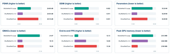
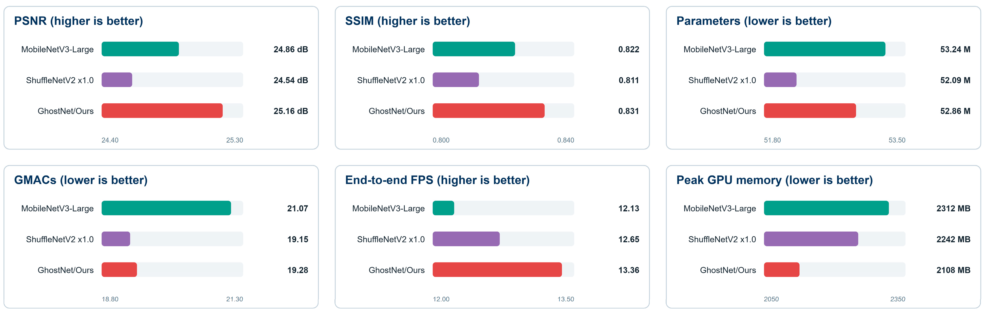
At the 32 × 32 and 64 × 64 stages, the factorized all-pairs term N2C contributes 0.537 and 4.295 GMACs, respectively (4.832 GMACs in total), while the two 3 × 3 HW → 64 → 2 convolution pairs contribute 10.274 GMACs. With the configured reduction ratio of 8, the coordinate attention 1 × 1 projections contribute 0.554 GMACs. The exact itemized CACM MAC subtotal is 15.659041 GMACs and is reported as 15.659 GMACs after rounding the exact subtotal to three decimals. Summing the individually rounded components (4.832 + 10.274 + 0.554) would yield 15.660 GMACs; this 0.001-GMAC difference is solely a rounding-order effect. Coordinate pooling, batch normalization, activations, and elementwise attention reweighting are non-MAC operations and are excluded. The nine-offset aggregation requires approximately 0.143 G scalar additions; these additions are reported separately and are explicitly excluded from the 19.28 GMAC total. The complete GhostNet/ours pipeline requires 19.28 GMACs and contains 52.86 M parameters for one input image pair. The full-pipeline accuracy–efficiency trade-offs of the three lightweight backbones are summarized in Figure 5.
Figure 5.
Full-pipeline accuracy and efficiency comparison of lightweight backbones under the stated giga multiply-accumulate operation (GMAC), runtime, and memory protocol.
For the controlled backbone comparison, all three variants use the same complete end-to-end pipeline and the full-pipeline MAC protocol described above. The reported parameter and MAC counts are computed under the same scope, covering the backbone, TCA, factorized CACM correlation, coordinate attention, regression heads, TPS sampling, dynamic canvas construction, and fusion. Accordingly, Table 2 summarizes the source-reported model size and computation at 512 × 512 input resolution; for GhostNet/Ours, the primary full-system complexity is consistent with that used in the controlled-backbone comparison. The PSNR and SSIM values in the controlled-backbone comparison are obtained from independently trained backbone control runs and are therefore reported separately from the primary benchmark result in Table 1.
Table 2.
Source-reported model size and computation at 512 × 512 input resolution.
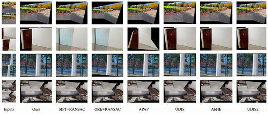
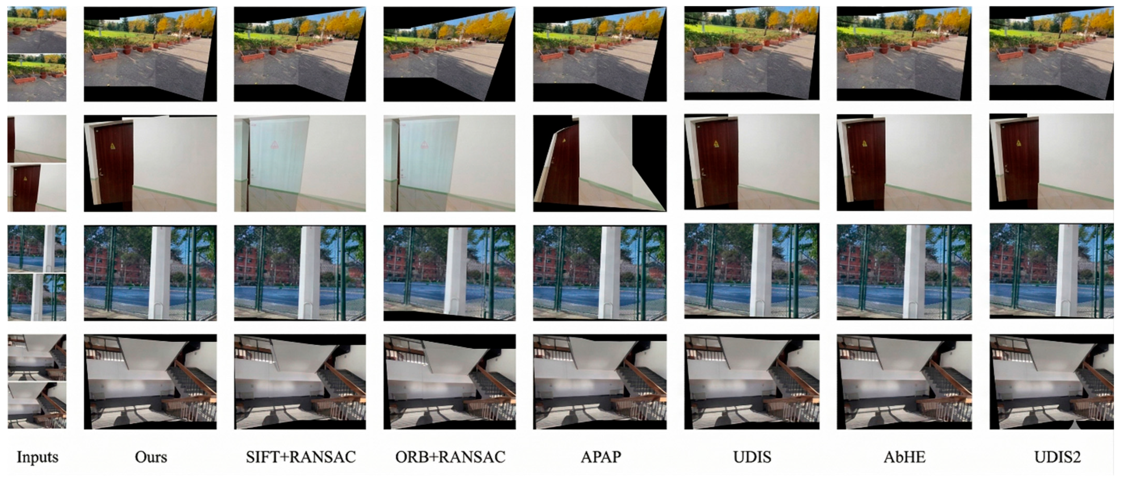
Figure 6 presents four selected UDIS-D examples covering outdoor planar structure, indoor low-texture regions, repeated vertical structures, and staircase geometry. Every method is shown for the same input pair in each row; black regions denote invalid canvas areas after warping.
Figure 6.
Qualitative stitching comparison on selected UDIS-D test pairs.
4.4. Ablation Studies
Table 3 presents the individual and joint ablation results for TCA and CACM under the same evaluation protocol. Removing TCA decreases PSNR from 25.19 to 24.13 dB and SSIM from 0.833 to 0.810, while removing CACM reduces PSNR to 24.09 dB and SSIM to 0.800. When both TCA and CACM are removed, the performance further decreases to 23.38 dB PSNR and 0.782 SSIM. Compared with this joint baseline, the complete model improves PSNR by 1.81 dB and SSIM by 0.051. These results demonstrate the benefit of combining TCA and CACM, while the individual ablations quantify the contribution of each module when the other is retained.
Table 3.
Module-level and joint module ablation on UDIS-D under the unified protocol.
4.5. Component and Lightweight-Backbone Analysis
Table 4 presents fine-grained component ablations, with the complete model (25.19 dB PSNR and 0.833 SSIM) serving as the reference. Replacing the dual GAP+GMP token construction with GAP alone decreases PSNR by 0.33 dB and SSIM by 0.008. Removing coordinate attention from CACM results in a larger reduction of 0.58 dB in PSNR and 0.021 in SSIM. Removing the mesh-shape regularization terms decreases PSNR by 0.44 dB and SSIM by 0.014. Section 4.7 further examines the individual contributions of the alignment and regularization terms.
Table 4.
Fine-grained component ablation on UDIS-D.
Under the unified full-pipeline comparison, GhostNet/ours achieves 25.16 dB PSNR and 0.831 SSIM, compared with 24.86/0.822 for MobileNetV3-Large and 24.54/0.811 for ShuffleNetV2 × 1.0. GhostNet/ours has intermediate parameter and MAC counts of 52.86 M and 19.28 GMACs, respectively, while providing the highest throughput at 13.36 FPS and the lowest peak GPU memory usage of 2108 MB. The accuracy values in Table 5 are obtained from independently trained backbone control runs, whereas the complexity values follow the same complete-pipeline profiling scope as Table 2.
Table 5.
Full-pipeline comparison of lightweight backbones at 512 × 512 input resolution under the unified GMAC, runtime, and memory protocol.
4.6. Runtime and Failure Analysis
Runtime and memory measurements for the complete backbone variants are presented in Table 5 under a unified GPU evaluation protocol. Traditional feature-matching baselines are evaluated separately in Table 6, where failed geometric estimates are retained in the all-sample results using identity-warp replacement and valid-only metrics are also provided. Table 7, Table 8, Table 9 and Table 10 present additional analyses of loss-term ablations, hyperparameter sensitivity, geometric-stage effectiveness, and mesh-cell orientation behavior.
Table 6.
Failure statistics and reconstruction metrics for traditional feature-matching methods on 1106 UDIS-D test pairs. Failed estimates use an identity warp in the all-sample aggregate.
Table 7.
Fine-grained loss-term ablation on UDIS-D.
Table 8.
One-factor-at-a-time sensitivity analysis of loss weights on UDIS-D.
Table 9.
Geometric-stage ablation on UDIS-D.
Table 10.
Two-triangle orientation-reversal/degeneration flag audit on the 1106-pair UDIS-D test set.
The observed failure-rate ordering is ORB+RANSAC, SIFT+RANSAC, and APAP from highest to lowest. For every method, valid-only PSNR/SSIM exceeds the all-sample result because failed estimates are retained through identity-warp replacement. APAP provides the best traditional valid-only result (23.41 dB, 0.728), but it remains below the complete model by 1.78 dB PSNR and 0.105 SSIM. This comparison documents the limitations of hand-crafted matching under the stated protocol; it does not constitute a paired significance test.
4.7. Additional Ablation, Sensitivity, and Mesh-Cell Orientation Analysis
Table 7 decomposes the objective under the complete architecture. Removing Lintra and Linter individually decreases PSNR by 0.19 dB and 0.25 dB, respectively, while removing both mesh regularizers results in a 0.44 dB decrease. The alignment terms have larger effects: removing LTPS decreases PSNR by 1.07 dB, whereas removing LH decreases PSNR by 0.72 dB. These results indicate that both global homography and local TPS supervision contribute substantially to the training objective, with LTPS showing the larger performance impact in this loss-term ablation.
Table 8 varies one weight at a time around the implemented setting. The default configuration (λ = 3, ω1 = 1, ω2 = 10) yields the highest PSNR and SSIM among the tested values in all three sweeps. Across these tested local variations, PSNR changes by no more than 0.30 dB and SSIM by no more than 0.009, indicating that the model performance remains reasonably stable under moderate perturbations of the loss weights. These results support the local robustness of the selected configuration within the evaluated parameter ranges.
The homography-only baseline in Table 9 was trained independently from scratch with exactly the same training protocol as the full model, including the identical UDIS-D training split, data augmentation, AdamW optimizer, exponential learning rate decay, batch size of 4, and 100-epoch schedule. The TPS control-point regression branch and all three TPS-related loss terms (, , ) were removed from the training objective. The model predicts only the four-corner homography offsets and uses the solved global homography as the final warp transformation, with no subsequent local refinement. The final checkpoint at epoch 100 is selected for evaluation, following the same fixed schedule as the complete model.
Table 9 evaluates the contribution of the second geometric stage. The homography-only baseline achieves 24.25 dB PSNR and 0.807 SSIM, whereas introducing TPS refinement improves the performance to 25.19 dB and 0.833, corresponding to gains of 0.94 dB in PSNR and 0.026 in SSIM. These results demonstrate the benefit of local TPS refinement following global homography initialization. The homography-only result is slightly higher than that of the w/o LTPS variant because the two experiments modify different components: the former removes the TPS stage entirely, whereas the latter retains TPS deformation but removes its direct alignment supervision. Therefore, the two results are not directly equivalent ablations.
Mathematical criterion for flagging locally reversed or degenerate control-mesh triangles. For each cell of the 12 × 12 mesh, let the following vectors denote its top-left, top-right, bottom-left, and bottom-right vertices, respectively:
Using upper-left-origin image coordinates with the vertical axis pointing downward, the two-dimensional cross product is defined as follows:
The implementation splits the quadrilateral along the diagonal connecting the top-right and bottom-left vertices and evaluates the two consistently oriented triangle signs:
Both quantities are positive for the regular initial grid. A cell is flagged when at least one triangle is locally orientation-reversed or degenerate:
The non-strict threshold matches the implemented audit: a negative triangle sign indicates orientation reversal, whereas a zero sign indicates triangle degeneration. This is a local control-mesh vertex audit and does not constitute a continuous Jacobian-sign or higher-order self-intersection audit of the TPS transformation.
For overlap-region classification, let denote the validity mask obtained by bilinearly warping an all-one tensor into the reference-image coordinate domain, with values in . Let denote the fixed cell-aligned raster block produced by the non-overlapping unfold operation. Its mean validity is as follows:
A cell is classified as belonging to the overlap region when we find the following:
The implementation uses non-overlapping 42 × 42 blocks with stride 42. Consequently, the 12 × 12 blocks cover the upper-left 504 × 504 region of each 512 × 512 mask; the final eight rows and final eight columns are not included in any block mean. The overlap criterion is defined for reproducibility, but we do not report a flag–overlap cross-tabulation because the retained audit output does not preserve the required cell-wise joint labels.
Using the above two-triangle criterion, all 1106 test images contain at least one flagged cell. In total, 11,586 of the 159,264 evaluated control-mesh cells are flagged (7.275%), corresponding to a mean of 10.476 flagged cells per image and a maximum of 37 in one image. The retained audit does not distinguish strict orientation reversals (s < 0) from zero-area degeneracies (s = 0); therefore, 11,586 denotes flagged cells and must not be interpreted as a count of folded cells. Because flags occur in every test image and in 7.275% of cells, the incidence of local orientation or area violations under this criterion is non-negligible. Such flags may indicate locally inverted or collapsed control-mesh triangles and potential geometric distortion. However, the number of true fold-overs and their direct effect on stitched-image quality cannot be determined without separate s < 0 and s = 0 counts or a continuous TPS-Jacobian audit. Future audits should retain the two categories and cell-wise spatial labels separately.
5. Conclusions
This work presents a coarse-to-fine image-stitching framework that integrates a shared GhostNet backbone, TCA-based multi-scale feature fusion, CACM-based correlation enhancement, global homography estimation, and local TPS refinement. TCA combines global-average and global-maximum channel descriptors to enhance feature representation, while CACM incorporates local correlation support and coordinate-aware reweighting to improve spatial correspondence modeling.
On UDIS-D, the complete model achieves 25.19 dB PSNR and 0.833 SSIM. Removing both TCA and CACM reduces the performance to 23.38 dB and 0.782, respectively, demonstrating the contribution of the proposed feature-enhancement modules. Loss-term ablations further show that both homography and TPS supervision are important to alignment accuracy, while the homography-only comparison confirms the additional benefit of local TPS refinement. The one-factor-at-a-time sensitivity analysis indicates stable performance within the evaluated loss-weight ranges, and the two-triangle orientation-reversal/degeneration flag audit identifies a non-negligible incidence of local control-mesh orientation or area violations under the stated criterion.
In the controlled backbone comparison, the GhostNet-based model achieves the highest reconstruction accuracy, the highest throughput of 13.36 FPS, and the lowest peak GPU memory usage of 2108 MB among the evaluated backbone variants, while maintaining moderate parameter and computational complexity under the stated GMAC, runtime, and memory protocol. The traditional feature-matching baselines also exhibit non-negligible geometric-estimation failures, highlighting the practical robustness advantage of the learning-based framework under the evaluated protocol.
Several limitations remain. The current evaluation is restricted to a single dataset and relies primarily on overlap-region PSNR and SSIM. Cross-dataset generalization, CPU and embedded-device profiling, perceptual seam-quality evaluation, and paired statistical analysis have not yet been investigated. In addition, the audit does not separate strict reversals (s < 0) from zero-area degeneracies (s = 0) and is not a continuous TPS-Jacobian analysis; it therefore cannot determine the number of true fold-overs, their direct image-level impact, or global TPS invertibility. Future work will therefore focus on broader cross-domain validation, deployment-oriented efficiency evaluation, perceptual stitching quality, separate orientation/degeneration reporting, and stronger geometric constraints for locally adaptive warping.
Author Contributions
Conceptualization, Y.W.; methodology, Z.H.; formal analysis, H.H.; investigation, H.H. and Z.H.; writing—original draft preparation, H.H. and Z.H.; writing—review and editing, Y.W.; visualization, Z.H.; supervision, Y.H.; project administration, Y.H.; funding acquisition, Y.W. All authors have read and agreed to the published version of the manuscript.
Funding
This research was funded by the Natural Science Foundation of Fujian Province of China, grant number 2022HZ022019.
Data Availability Statement
The UDIS-D dataset used in this study is publicly available from its original source. No new dataset was created for this work. The complete implementation is not publicly available at present because the training and evaluation repository requires project-specific dependency cleanup. Requests for research access may be directed to the corresponding author.
Conflicts of Interest
The authors declare no conflicts of interest.
Abbreviations
The following abbreviations are used in this manuscript:
| FoV | Field of view |
| TCA | Transformer-based channel attention |
| CACM | Coordinate-aware correlation module |
| SIFT | Scale-invariant feature transform |
| CNN | Convolutional neural network |
| TPS | Thin plate spline |
| GAP | Global average pooling |
| GMP | Global max pooling |
| MLP | Multi-layer perceptron |
| CA | Coordinate attention |
| PSNR | Peak signal-to-noise ratio |
| SSIM | Structural similarity index measure |
References
- Ni, J.; Chen, Y.; Chen, Y.; Zhu, J.; Ali, D.; Cao, W. A Survey on Theories and Applications for Self-Driving Cars Based on Deep Learning Methods. Appl. Sci. 2020, 10, 2749. [Google Scholar] [CrossRef] [Scilit]
- Ye, Z.; Shao, C.; Zhu, K. Unsupervised Neural Network-Based Image Stitching Method for Bladder Endoscopy. PLoS ONE 2025, 20, e0311637. [Google Scholar] [CrossRef] [Scilit]
- Li, J.; Zhao, Y.; Ye, W.; Yu, K.; Ge, S. Attentive Deep Stitching and Quality Assessment for 360° Omnidirectional Images. IEEE J. Sel. Top. Signal Process. 2019, 14, 209–221. [Google Scholar] [CrossRef] [Scilit]
- Brown, M.; Lowe, D.G. Automatic Panoramic Image Stitching Using Invariant Features. Int. J. Comput. Vis. 2007, 74, 59–73. [Google Scholar] [CrossRef] [Scilit]
- Xiang, T.-Z.; Xia, G.-S.; Bai, X.; Zhang, L. Image Stitching by Line-Guided Local Warping with Global Similarity Constraint. Pattern Recognit. 2018, 83, 481–497. [Google Scholar] [CrossRef] [Scilit]
- Jia, Q.; Li, Z.; Fan, X.; Zhao, H.; Teng, S.; Ye, X.; Latecki, L.J. Leveraging Line-Point Consistence to Preserve Structures for Wide Parallax Image Stitching. In Proceedings of the IEEE/CVF Conference on Computer Vision and Pattern Recognition, Nashville, TN, USA, 20–25 June 2021; IEEE: New York, NY, USA, 2021; pp. 12186–12195. [Google Scholar]
- Du, P.; Ning, J.; Cui, J.; Huang, S.; Wang, X.; Wang, J. Geometric Structure Preserving Warp for Natural Image Stitching. In Proceedings of the IEEE/CVF Conference on Computer Vision and Pattern Recognition, New Orleans, LA, USA, 18–24 June 2022; IEEE: New York, NY, USA, 2022; pp. 3688–3696. [Google Scholar]
- Liao, T.; Li, N. Natural Image Stitching Using Depth Maps. arXiv 2022, arXiv:2202.06276. [Google Scholar]
- Li, A.; Guo, J.; Guo, Y. Image Stitching Based on Semantic Planar Region Consensus. IEEE Trans. Image Process. 2021, 30, 5545–5558. [Google Scholar] [CrossRef] [Scilit]
- DeTone, D.; Malisiewicz, T.; Rabinovich, A. Deep Image Homography Estimation. arXiv 2016, arXiv:1606.03798. [Google Scholar]
- Nguyen, T.; Chen, S.W.; Shivakumar, S.S.; Taylor, C.J.; Kumar, V. Unsupervised Deep Homography: A Fast and Robust Homography Estimation Model. IEEE Robot. Autom. Lett. 2018, 3, 2346–2353. [Google Scholar] [CrossRef] [Scilit]
- Zhang, J.; Wang, C.; Liu, S.; Jia, L.; Ye, N.; Wang, J.; Zhou, J.; Sun, J. Content-Aware Unsupervised Deep Homography Estimation. In Proceedings of the European Conference on Computer Vision, Glasgow, UK, 23–28 August 2020; Springer: Cham, Switzerland, 2020; pp. 653–669. [Google Scholar]
- Nie, L.; Lin, C.; Liao, K.; Liu, S.; Zhao, Y. Unsupervised Deep Image Stitching: Reconstructing Stitched Features to Images. IEEE Trans. Image Process. 2021, 30, 6184–6197. [Google Scholar] [CrossRef] [Scilit]
- Hong, M.; Lu, Y.; Ye, N.; Lin, C.; Zhao, Q.; Liu, S. Unsupervised Homography Estimation with Coplanarity-Aware GAN. In Proceedings of the IEEE/CVF Conference on Computer Vision and Pattern Recognition, New Orleans, LA, USA, 18–24 June 2022; IEEE: New York, NY, USA, 2022; pp. 17663–17672. [Google Scholar]
- Kweon, H.; Kim, H.; Kang, Y.; Yoon, Y.; Jeong, W.; Yoon, K.-J. Pixel-Wise Warping for Deep Image Stitching. In Proceedings of the AAAI Conference on Artificial Intelligence, Washington, DC, USA, 7–14 February 2023; pp. 1196–1204. [Google Scholar]
- Kim, M.; Lee, J.; Lee, B.; Im, S.; Jin, K.H. Implicit Neural Image Stitching with Enhanced and Blended Feature Reconstruction. In Proceedings of the IEEE/CVF Winter Conference on Applications of Computer Vision, Waikoloa, HI, USA, 3–8 January 2024; IEEE: New York, NY, USA, 2024; pp. 4087–4096. [Google Scholar] [CrossRef] [Scilit]
- Huo, M.; Zhang, Z.; Ren, X.; Yang, X.; Ye, C. AbHE: All Attention-Based Homography Estimation. IEEE Trans. Instrum. Meas. 2024, 73, 1–11. [Google Scholar] [CrossRef] [Scilit]
- Gao, J.; Kim, S.J.; Brown, M.S. Constructing Image Panoramas Using Dual-Homography Warping. In Proceedings of the IEEE Conference on Computer Vision and Pattern Recognition, Colorado Springs, CO, USA, 20–25 June 2011; ACM Digital Library: New York, NY, USA, 2011; pp. 49–56. [Google Scholar]
- Lin, W.-Y.; Liu, S.; Matsushita, Y.; Ng, T.-T.; Cheong, L.-F. Smoothly Varying Affine Stitching. In Proceedings of the IEEE Conference on Computer Vision and Pattern Recognition, Colorado Springs, CO, USA, 20–25 June 2011; ACM Digital Library: New York, NY, USA, 2011; pp. 345–352. [Google Scholar]
- Zaragoza, J.; Chin, T.-J.; Brown, M.S.; Suter, D. As-Projective-as-Possible Image Stitching with Moving DLT. In Proceedings of the IEEE Conference on Computer Vision and Pattern Recognition, Portland, OR, USA, 23–28 June 2013; IEEE: New York, NY, USA, 2013; pp. 2339–2346. [Google Scholar]
- Nie, L.; Lin, C.; Liao, K.; Liu, S.; Zhao, Y. Depth-Aware Multi-Grid Deep Homography Estimation with Contextual Correlation. IEEE Trans. Circuits Syst. Video Technol. 2021, 32, 4460–4472. [Google Scholar] [CrossRef] [Scilit]
- Nie, L.; Lin, C.; Liao, K.; Liu, S.; Zhao, Y. Parallax-Tolerant Unsupervised Deep Image Stitching. In Proceedings of the IEEE/CVF International Conference on Computer Vision, Paris, France, 1–6 October 2023; IEEE: New York, NY, USA, 2023; pp. 7399–7408. [Google Scholar]
- Hou, Q.; Zhou, D.; Feng, J. Coordinate Attention for Efficient Mobile Network Design. In Proceedings of the IEEE/CVF Conference on Computer Vision and Pattern Recognition, Nashville, TN, USA, 20–25 June 2021; IEEE: New York, NY, USA, 2021; pp. 13713–13722. [Google Scholar]
- Han, K.; Wang, Y.; Tian, Q.; Guo, J.; Xu, C.; Xu, C. GhostNet: More Features from Cheap Operations. In Proceedings of the IEEE/CVF Conference on Computer Vision and Pattern Recognition, Seattle, WA, USA, 13–19 June 2020; IEEE: New York, NY, USA, 2020; pp. 1580–1589. [Google Scholar]
- Chollet, F. Xception: Deep Learning with Depthwise Separable Convolutions. In Proceedings of the IEEE Conference on Computer Vision and Pattern Recognition, Honolulu, HI, USA, 21–26 July 2017; IEEE: New York, NY, USA, 2017; pp. 1251–1258. [Google Scholar]
- Bay, H.; Ess, A.; Tuytelaars, T.; Van Gool, L. Speeded-Up Robust Features (SURF). Comput. Vis. Image Underst. 2008, 110, 346–359. [Google Scholar] [CrossRef] [Scilit]
- Rosten, E.; Porter, R.; Drummond, T. Faster and Better: A Machine Learning Approach to Corner Detection. IEEE Trans. Pattern Anal. Mach. Intell. 2008, 32, 105–119. [Google Scholar] [CrossRef] [Scilit]
- Rublee, E.; Rabaud, V.; Konolige, K.; Bradski, G. ORB: An Efficient Alternative to SIFT or SURF. In Proceedings of the IEEE International Conference on Computer Vision, Barcelona, Spain, 6–13 November 2011; IEEE: New York, NY, USA, 2011; pp. 2564–2571. [Google Scholar]
- Liu, W.X.; Chin, T.-J. Correspondence Insertion for As-Projective-as-Possible Image Stitching. arXiv 2016, arXiv:1608.07997. [Google Scholar]
- Chang, C.-H.; Sato, Y.; Chuang, Y.-Y. Shape-Preserving Half-Projective Warps for Image Stitching. In Proceedings of the IEEE Conference on Computer Vision and Pattern Recognition, Columbus, OH, USA, 23–28 June 2014; IEEE: New York, NY, USA, 2014; pp. 3254–3261. [Google Scholar]
- Lin, C.-C.; Pankanti, S.U.; Natesan Ramamurthy, K.; Aravkin, A.Y. Adaptive As-Natural-as-Possible Image Stitching. In Proceedings of the IEEE Conference on Computer Vision and Pattern Recognition, Boston, MA, USA, 7–12 June 2015; IEEE: New York, NY, USA, 2015; pp. 1155–1163. [Google Scholar]
- Chen, Y.-S.; Chuang, Y.-Y. Natural Image Stitching with the Global Similarity Prior. In Proceedings of the European Conference on Computer Vision, Amsterdam, The Netherlands, 11–14 October 2016; Springer: Cham, Switzerland, 2016; pp. 186–201. [Google Scholar]
- Kim, M.; Lee, Y.; Han, W.K.; Jin, K.H. Learning Residual Elastic Warps for Image Stitching under Dirichlet Boundary Condition. In Proceedings of the IEEE/CVF Winter Conference on Applications of Computer Vision, Waikoloa, HI, USA, 3–8 January 2024; IEEE: New York, NY, USA, 2024; pp. 4016–4024. [Google Scholar] [CrossRef] [Scilit]
- Chen, K.; Garg, A.; Wang, Y.-S. Seamless-Through-Breaking: Rethinking Image Stitching for Optimal Alignment. In Computer Vision—ACCV 2024; Lecture Notes in Computer Science; Springer: Singapore, 2025; Volume 15476, pp. 455–469. [Google Scholar] [CrossRef] [Scilit]
- Liao, T.; Zhao, C.; Li, L.; Cao, H. Leveraging Local Patch Alignment to Seam-Cutting for Large Parallax Image Stitching. In Proceedings of the IEEE/CVF International Conference on Computer Vision, Honolulu, HI, USA, 19–23 October 2025; IEEE: New York, NY, USA, 2025; pp. 27262–27271. [Google Scholar] [CrossRef] [Scilit]
- Shao, M.; Tasdizen, T.; Joshi, S. Analyzing the Domain Shift Immunity of Deep Homography Estimation. In Proceedings of the IEEE/CVF Winter Conference on Applications of Computer Vision, Waikoloa, HI, USA, 3–8 January 2024; IEEE: New York, NY, USA, 2024; pp. 4800–4808. [Google Scholar] [CrossRef] [Scilit]
- Howard, A.; Sandler, M.; Chu, G.; Chen, L.-C.; Chen, B.; Tan, M.; Wang, W.; Zhu, Y.; Pang, R.; Vasudevan, V.; et al. Searching for MobileNetV3. In Proceedings of the IEEE/CVF International Conference on Computer Vision, Seoul, Republic of Korea, 27 October–2 November 2019; pp. 1314–1324. [Google Scholar] [CrossRef] [Scilit]
- Ma, N.; Zhang, X.; Zheng, H.-T.; Sun, J. ShuffleNet V2: Practical Guidelines for Efficient CNN Architecture Design. In Proceedings of the European Conference on Computer Vision, Munich, Germany, 8–14 September 2018; Springer: Cham, Switzerland, 2018; pp. 116–131. [Google Scholar]
- Jia, Q.; Li, Z.; Fan, X.; Zhao, H.; Teng, S.; Ye, X.; Latecki, L.J. Learning Pixel-wise Alignment for Unsupervised Image Stitching. In Proceedings of ACM Multimedia, Ottawa, ON, Canada, 29 October–3 November 2023; ACM: New York, NY, USA, 2023; pp. 1392–1400. [Google Scholar] [CrossRef] [Scilit]
- Fan, X.; Sun, L.; Zhang, Z.; Durrani, T.S. Progressive Alignment and Interwoven Composition Network for Image Stitching. Complex Intell. Syst. 2025, 11, 90. [Google Scholar] [CrossRef] [Scilit]
- Zhang, Y.; Ruan, B.; Du, L.; Li, L.; Li, Z.; Wang, X.; Xiao, J. Hierarchical Grid-Constrained Fusion Network for Image Stitching. J. King Saud Univ. Comput. Inf. Sci. 2025, 37, 17. [Google Scholar] [CrossRef] [Scilit]
- Jin, H.; Nie, L.; Lin, C.; Feng, X.; Zhao, Y. PixelStitch: Structure-Preserving Pixel-Wise Bidirectional Warps for Unsupervised Image Stitching. In Proceedings of the IEEE/CVF International Conference on Computer Vision, Honolulu, HI, USA, 19–23 October 2025; IEEE: New York, NY, USA, 2025; pp. 28125–28134. [Google Scholar] [CrossRef] [Scilit]
- Liao, T.; Zhao, C.; Li, L.; Cao, H. Parallax-Tolerant Image Stitching via Segmentation-Guided Multi-Homography Warping. Signal Process. 2025, 230, 109860. [Google Scholar] [CrossRef] [Scilit]
- Liao, T.; Li, N. Natural Image Stitching Using Depth Maps. Signal Process. Image Commun. 2026, 141, 117438. [Google Scholar] [CrossRef] [Scilit]
- Huang, Z.; Wu, Y. Attention-Guided Multi-Scale Fusion for Accurate Image Stitching. In Proceedings of the 2025 International Conference on Computer Vision, Image Processing and Computational Photography (CVIP 2025), Hangzhou, China, 17–19 October 2025; IEEE: New York, NY, USA, 2025; pp. 223–226. Available online: https://ieeexplore.ieee.org/document/11291287 (accessed on 30 August 2026).
- Kent, J.T.; Mardia, K.V. The Link between Kriging and Thin-Plate Splines. In Probability, Statistics and Optimization; Wiley: New York, NY, USA, 1994; pp. 326–339. [Google Scholar]

Disclaimer/Publisher’s Note: The statements, opinions and data contained in all publications are solely those of the individual author(s) and contributor(s) and not of MDPI and/or the editor(s). MDPI and/or the editor(s) disclaim responsibility for any injury to people or property resulting from any ideas, methods, instructions or products referred to in the content. |
© 2026 by the authors. Licensee MDPI, Basel, Switzerland. This article is an open access article distributed under the terms and conditions of the Creative Commons Attribution (CC BY) license.