A Memory-Efficient Depthwise Separable Convolution Accelerator Using Run-Length Coding

Abstract

On edge devices, convolutional neural network (CNN) inference is bottlenecked mainly by memory bandwidth, owing to the frequent memory accesses to feature maps and parameters. To address this challenge, we propose a memory-efficient hardware accelerator for depthwise separable convolution that minimizes off-chip memory traffic and parameter storage. The proposed architecture employs three key techniques: (1) a 64-bit run-length coding (RLC) packet compression that exploits feature-map sparsity after ReLU, (2) a mixed-precision scheme that represents feature maps and weights at different precisions, and (3) separated depthwise and pointwise convolution units. In particular, feature maps are transferred in RLC-compressed form, which reduces the amount of data exchanged with the host. The compressed data are decoded row by row, so the on-chip buffers hold only the rows required for computation rather than a complete feature map. In software simulation on ImageNet, the mixed-precision scheme reduced the parameter storage by 49.22% at a cost of 6.24 percentage points (pp) in Top-1 accuracy, and the RLC reduced the data by up to 56.07% in the deeper layers. Implemented on a Xilinx ZCU-104 FPGA, the proposed accelerator performs the depthwise separable convolution with a small number of logic resources and on-chip memory, confirming its feasibility for resource-constrained edge devices.

1. Introduction

With the rapid growth of deep learning applications, edge computing has emerged as a critical paradigm for real-time inference at the device level. By performing computation locally rather than offloading data to cloud servers, edge computing reduces latency and reliance on network connectivity, and minimizes power consumption. Accordingly, the demand for edge AI is growing across diverse domains, including smart manufacturing, autonomous driving, and wearable devices [1,2,3,4,5,6,7,8]. Vision-based applications such as image classification and object detection rely on convolutional neural networks (CNNs), which extract hierarchical features from input images through successive convolution operations [9]. However, CNNs impose substantial computational and memory access costs, making real-time inference on resource-constrained edge devices impractical and energy-inefficient. Consequently, lightweight techniques that reduce computational complexity while preserving accuracy are essential for practical deployment.

MobileNetV1 was proposed as a representative lightweight model to address this challenge [10]. By replacing standard convolutions with depthwise separable convolution (DSC), MobileNetV1 decomposes each convolution into a depthwise convolution (DWC) and a pointwise convolution (PWC), where DW and PW are used hereafter as modifiers for the parameters and processing elements of each operation, reducing the computational complexity. Hardware accelerator designs targeting this architecture have been actively investigated [11,12,13,14,15,16]. Nevertheless, model-level compression alone cannot fully eliminate hardware-level bottlenecks, particularly the memory access latency and data transfer bandwidth constraints that arise during CNN inference. Since repeated accesses to feature maps and parameters constitute a significant fraction of total power consumption, improving memory access and data transfer efficiency at the hardware level is essential [17].

We propose a memory-efficient hardware accelerator for depthwise separable convolution that minimizes off-chip memory traffic and parameter storage in resource-constrained environments. Specifically, the proposed architecture applies the following three techniques, each at the point and in the form determined by the characteristics of the target model and the constraints of the hardware.

• Run-Length Coding-based compressed data transfer. We apply Run-Length Coding (RLC) to input feature maps, transmitting and storing data as compressed 64-bit packets during off-chip memory transfers to reduce data transfer.
• Mixed-precision quantization. We adopt a mixed-precision quantization policy in which feature maps and depthwise (DW) weights are represented in FP16, while pointwise (PW) weights are quantized to FP8 (E5M2).
• Separated depthwise and pointwise convolution units. We design dedicated hardware engines for depthwise and pointwise convolution, integrated with the proposed RLC-based compressed data transfer and mixed-precision arithmetic.

By integrating these three techniques, the proposed accelerator reduces parameter storage by 49.22% and achieves an RLC compression ratio of up to 56.07% in the deeper layers on ImageNet, at a cost of 6.24 percentage points (pp) in Top-1 accuracy. The design is implemented in Verilog HDL on a Xilinx ZCU-104 FPGA and verified layer by layer against the software golden results, using 79.5k LUTs and 12.55 Mb of on-chip memory.

2. Background

2.1. MobileNetV1

MobileNetV1 is a lightweight CNN proposed by Google in 2017, designed for efficient deep learning inference in mobile and embedded environments [10]. Conventional CNNs such as VGG and ResNet require millions of parameters and a substantial amount of computation, making them difficult to deploy on edge devices with limited memory capacity and power budget [18,19]. To address this, MobileNetV1 introduces a computational structure called depthwise separable convolution, which substantially reduces both the amount of computation and the number of parameters while minimizing accuracy loss.

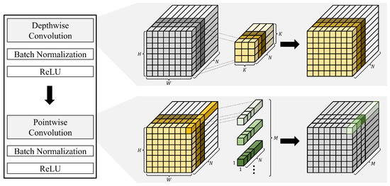
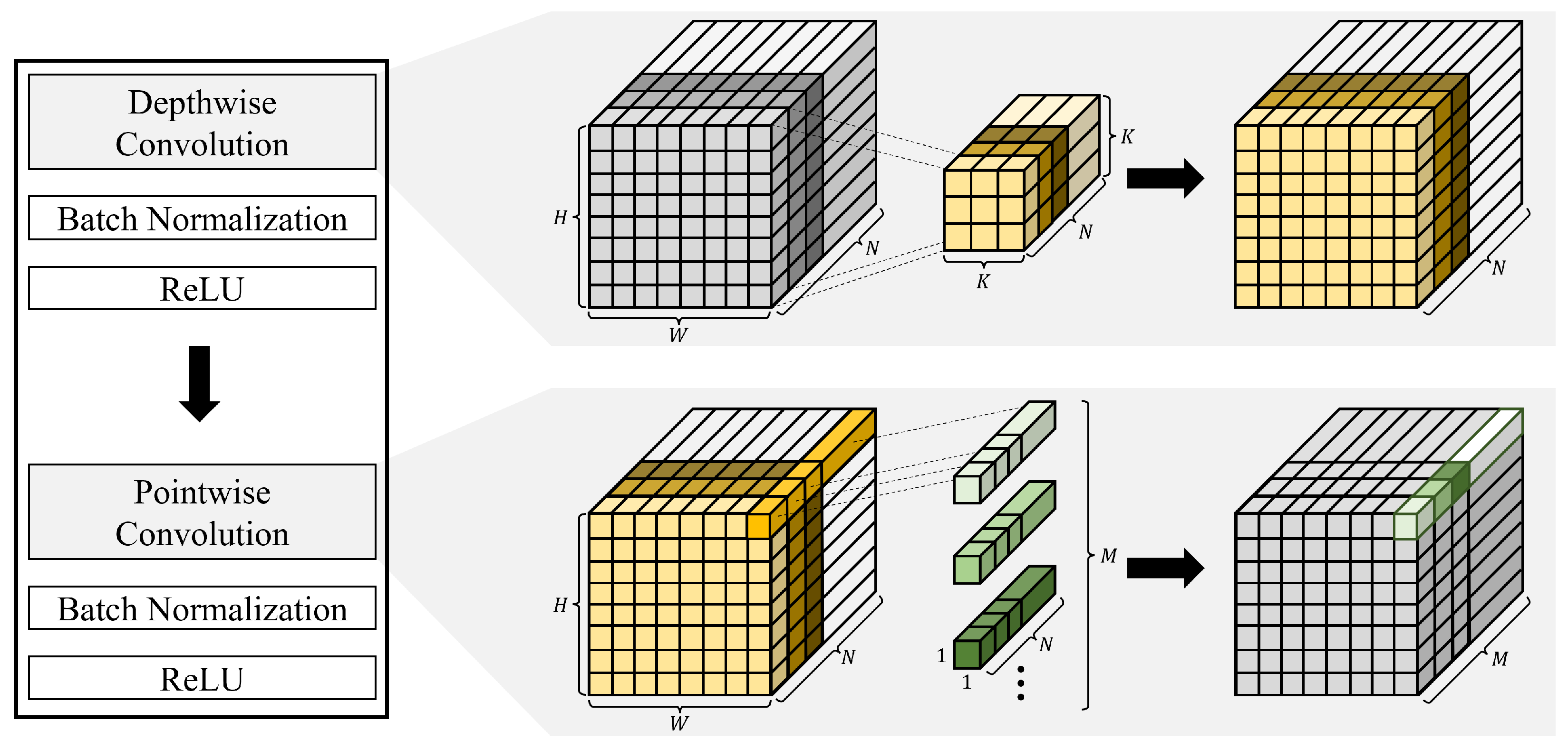
Figure 1 illustrates the depthwise separable convolution, the core operation of MobileNetV1. MobileNetV1 constructs the entire network by repeatedly stacking depthwise separable convolution blocks. Each block consists of a depthwise convolution, batch normalization, ReLU, pointwise convolution, batch normalization, and ReLU, in this order; as these blocks are stacked successively, the number of channels increases with depth. The key idea of depthwise separable convolution is to decompose the convolution into two stages. For a standard 2D convolution with N input channels, M output channels, and a kernel size of $K\times K$, the total computational cost is given by (1), where H and W denote the spatial dimensions of the feature map.

$$C_{\mathrm{std}}=K^2\times M\times N\times H\times W$$

(1)

Figure 1. Computational flow of Depthwise Separable Convolution.

In this structure, every output channel is connected to every input channel, resulting in a high computational cost. In contrast, depthwise separable convolution splits this operation into two stages. In the first stage, depthwise convolution applies one independent kernel to each input channel, decoupling the computation across channels and reducing the cost to (2).

$$C_{\mathrm{dw}}=K^2\times N\times H\times W$$

(2)

In the second stage, pointwise convolution applies a $1\times 1$ convolution to combine the depthwise outputs along the channel dimension, with the cost given by (3).

$$C_{\mathrm{pw}}=M\times N\times H\times W$$

(3)

Consequently, the total cost is reduced to $C_{\mathrm{dw}}+C_{\mathrm{pw}}$, and the computational reduction ratio relative to the standard convolution is expressed as (4).

$${\displaystyle \frac{C_{\mathrm{dw}}+C_{\mathrm{pw}}}{C_{\mathrm{std}}}}={\displaystyle \frac{1}{M}}+{\displaystyle \frac{1}{K^2}}$$

(4)

For example, when $K=3$ and $M=N=128$, the computation is reduced to approximately one-ninth.

2.2. Run-Length Coding

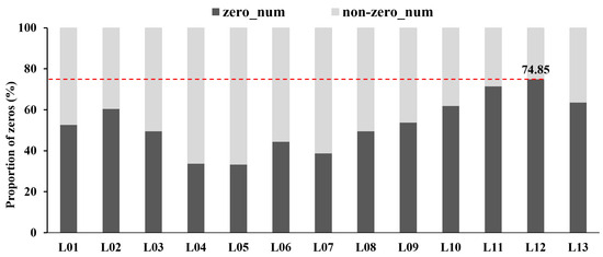
In deep convolutional neural networks such as MobileNetV1, the proportion of zero values in feature maps increases substantially with network depth. This phenomenon arises from the rectified linear unit (ReLU) activation function applied at each layer: ReLU maps all non-positive inputs to zero, causing a large fraction of feature-map values to become zero in the deeper layers. While this induced sparsity is an inherent property of the architecture, it leads to inefficient memory utilization and unnecessary bandwidth consumption, as zeros are repeatedly stored and transmitted between processing modules. Figure 2 shows the proportion of zero values in the input data at each layer of MobileNetV1; up to 74.85% of the input values at Layer 12 are zero, confirming that sparsity increases progressively toward deeper layers. Motivated by this observation, the proposed system adopts an RLC-based lossless compression scheme [20]. RLC encodes a sequence of repeated values by representing each run of identical elements as a (count, value) pair, thereby reducing the total data length. Applied to CNN feature maps where zeros occur frequently, RLC reduces both storage requirements and inter-module transmission bandwidth.

Figure 2. Proportion of zeros in the feature map of each layer of MobileNetV1, averaged over 1000 CIFAR-100 test samples. L01 denotes the first depthwise separable convolution (DSC) layer; the initial standard convolution layer of MobileNetV1 is excluded.

2.3. Mixed-Precision

In deep learning inference and training, tensors such as weights, biases, and feature maps are conventionally represented in floating-point format. Traditionally, 32-bit single-precision (FP32) has served as the standard; however, as model sizes grow and the demand for real-time edge inference increases, reduced-precision numeric formats have been actively studied as a means of lowering memory footprint and computational cost [21]. The simplest approach is to apply a uniform low-precision format (e.g., FP8) across the entire model. However, individual layers in a neural network exhibit different sensitivities to precision reduction. Indiscriminate application of low precision to sensitive layers causes a sharp accuracy drop, whereas insensitive layers incur negligible accuracy loss under the same reduction [22]. Exploiting this layer-wise sensitivity disparity, mixed precision retains high precision for sensitive operations while applying lower precision to less sensitive parameters. Adopting mixed precision improves hardware efficiency in three respects. First, in terms of memory reduction, storage requirements scale directly with bit width, so halving the bit width relative to FP32 reduces storage by half, and quartering it reduces storage by a quarter. Second, in terms of computational throughput, narrower bit widths allow more Multiply-Accumulate (MAC) units to be integrated within the same silicon area, thereby increasing throughput. Third, in terms of memory bandwidth, the reduced transfer size alleviates latency in memory-bound operations.

3. Related Work

Various hardware accelerators have been proposed to efficiently support depthwise separable convolution–based networks such as MobileNet. Because DWC and PWC exhibit markedly different computational and data-access characteristics, prior accelerators have explored a range of strategies that can be broadly grouped by whether they primarily target latency and throughput, hardware resource usage, or memory.

A widely adopted strategy is the separated architecture, which implements dedicated accelerators for DWC and PWC. Hong et al. [23] designed dedicated processing units for DWC and PWC, and observed that PWC requires considerably more computation time than DWC. They introduced a pipelining-separable-convolution scheme that overlaps the shorter DWC with the longer PWC; since DWC operates independently on each channel, it can begin as soon as partial PWC outputs are available, reducing the overall latency by 1.82×. They additionally partitioned the PWC input feature maps into tiles for parallel processing, improving throughput by 24.5–32×. Wu et al. [24] likewise employed two dedicated engines—a convolution engine for PWC and a depthwise-convolution engine—and scheduled them in a layer-wise pipeline so that the two operate in parallel. A channel-augmentation technique is also used to rearrange width-reused data into otherwise-empty channel dimensions, improving utilization in the first layer. These works mainly focus on computation architecture, latency, and throughput.

Another line of work aims to reduce hardware resource usage by reusing a single structure across operations and layers. Liao et al. [14] implemented configurable DWC and PWC units—with programmable weights, feature-map size, stride, and data path—so that a single computing structure processes all layers through reuse rather than dedicated per-layer circuits, achieving low resource consumption (e.g., 12.11% DSP and 4.21% LUT utilization). Ou et al. [25] constructed a single processing element (PE) array compatible with both DWC and PWC, switchable by reconfiguring the control signals and dataflow. They paired this array with a hybrid scheduling strategy that substantially improves on-chip storage utilization. Sang et al. [26] adopted a dynamically reconfigurable computing engine whose PEs switch between DWC and PWC modes, raising PE utilization so that more computation is performed with the same hardware resources. These works focus on processing diverse operations with a shared structure to lower the required hardware resources.

A third group of accelerators targets memory more directly. Lin et al. [27] proposed a low-memory MobileNet accelerator with configurable PWC and DWC accelerators that can be pipelined or bypassed, and minimized both on-chip memory capacity and on-chip/off-chip data transfer. Xuan et al. [28] processed the three sub-layers of a DSC block end-to-end rather than layer-by-layer, keeping intermediate feature maps in a small number of buffers and thereby reducing repeated memory accesses by 80.5%. They also dynamically allocated 16 PE arrays between the two PW layers according to their operation ratio, maintaining PE utilization above 85%. These memory-oriented designs reduce memory mainly through architectural and dataflow techniques—buffer reuse, scheduling, and end-to-end processing—whereas comparatively few exploit data-level compression. Rather than prioritizing computational throughput, this work focuses on reducing memory usage through RLC compression and mixed-precision computation, and presents a hardware accelerator architecture optimized around this objective.

4. The Proposed Architecture

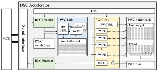
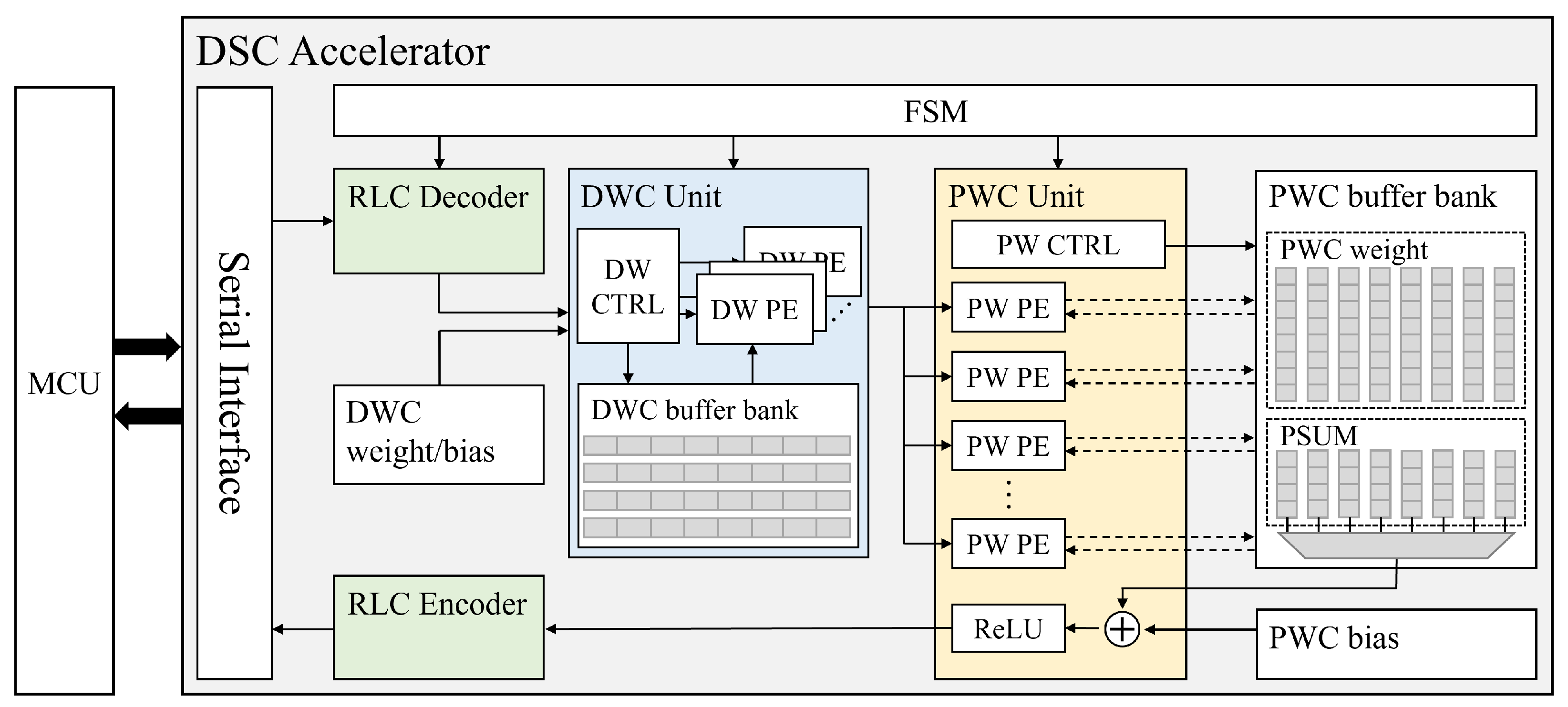
Figure 3 shows the overall block diagram of the proposed accelerator. The hardware comprises five main components: an RLC encoder, an RLC decoder, a depthwise convolution unit, a pointwise convolution unit, and a finite state machine (FSM). At the input and output stages, data are exchanged with the host through a serial peripheral interface (SPI). To eliminate batch normalization from the hardware datapath, the batch normalization parameters are folded into the preceding convolution weights and biases prior to deployment.

Figure 3. The overall block diagram of the proposed architecture.

The overall data flow proceeds as follows. The parameters required for computation are first received over SPI and stored in their respective memories. When the input feature map, compressed by the RLC algorithm, arrives, it passes through the RLC decoder and is stored in the DWC buffer bank. Once the data required to begin the depthwise convolution are ready, the DWC unit performs the depthwise convolution, and its result is forwarded to the PWC unit for the pointwise convolution. The computed output is then recompressed by the RLC encoder and transmitted off-chip. The FSM governs the overall data flow. The entire hardware system was designed and implemented in Verilog HDL.

The proposed accelerator adopts a mixed-precision scheme that combines FP16 and FP8. The feature maps and the depthwise weights and biases are kept in FP16, while the pointwise weights and biases are stored in FP8. Two 8-bit floating-point formats are in common use, E4M3 with a 4-bit exponent and a 3-bit mantissa, and E5M2 with a 5-bit exponent and a 2-bit mantissa. This work adopts E5M2 because it is directly compatible with the FP16 datapath. E4M3 uses a 4-bit exponent with a bias different from that of FP16, so converting an E4M3 value to FP16 requires re-biasing the exponent and normalizing subnormal values at every multiply lane. E5M2, in contrast, shares the sign bit and the 5-bit exponent field with FP16 using the same bias, so the corresponding FP16 value is obtained by appending eight zero bits to the mantissa. This expansion requires no arithmetic, and the FP16–FP8 mixed-precision computation is therefore performed with FP16 multipliers alone.

4.1. Run-Length Coding Module

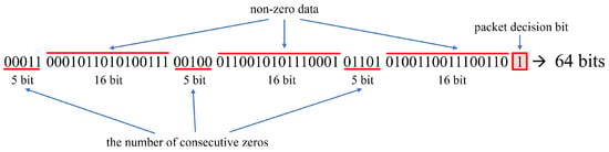
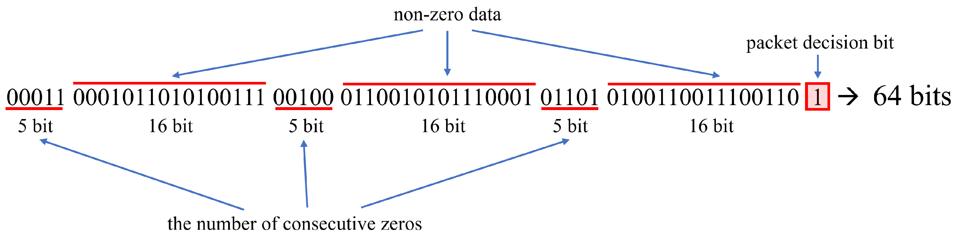
In this work, an RLC coding scheme based on a 64-bit packet structure is designed, and the packet layout is shown in Figure 4. To fully exploit the sparsity of CNN feature maps, the packet stores each run of consecutive zeros paired with the subsequent non-zero value. Specifically, a single packet can hold up to three zero runs and their interleaved non-zero values, where each pair is represented by a 5-bit zero count and a 16-bit value field. A pair whose 16-bit value field is zero does not carry a value and indicates that the zero run continues, so its zero count is accumulated with that of the following pair and a run longer than 31 is represented by more than one pair. Because zeros are always represented by the count field, the value field does not hold a zero, and marking a continued run therefore requires no additional bit within a pair. The least significant bit (LSB) serves as a packet decision bit, indicating whether the compressed data contain the end of a row of an input channel. For example, when an input channel is of size $112\times 112$, the packet decision bit is set to 1 to mark the completion of compression for a row of 112 elements. Since the number of original elements packed into a single packet varies with the data characteristics, restoring an exact number of elements in hardware is non-trivial; the proposed structure overcomes this by enabling straightforward row-wise reconstruction through the packet decision bit. When a row cannot be represented by three pairs, the pairs continue into the following packet, so a row is represented by a sequence of packets rather than by a single packet. The zeros that remain after the last non-zero value of a row are recorded only in complete groups of 31, and the zeros that do not complete such a group are not encoded; the decoder, which receives the row length as a runtime parameter of the layer, fills the remainder of the row with zeros once that length is reached. Unused pairs in the packet that terminates a row are set to zero. A row that contains only zeros is handled in the same way, and for the feature map sizes used in this work it is represented by a single packet with its packet decision bit set. All of these cases are handled by the same zero counter and packet decision bit, and require no additional logic in the encoder or the decoder. Furthermore, because the data are aligned on a per-packet basis, unnecessary buffer movement is minimized and a consistent processing timing is maintained during decompression. As a result, the proposed 64-bit RLC packet can represent up to 96 original elements in a single packet, achieving high compression efficiency. Conversely, when the data contain no zeros, each packet holds at most three elements, so encoding a row requires $\lceil W/3\rceil$ packets and the transfer size becomes $4\lceil W/3\rceil /W$ of the uncompressed size–equal to $4/3$ only when W is a multiple of three, and larger otherwise, reaching its largest value among the row widths used in this work at $W=7$, where it is $12/7$. Together with the single-packet case described above (transfer size $4/W$), the transfer size ranges from about $1/28$ ($W=114$) to $12/7$. The break-even zero proportion is likewise row-width dependent, equal to exactly 25% when W is a multiple of four and tending to be higher for narrower rows.

Figure 4. Proposed 64-bit Run-Length Coding Packet Structure.

The RLC decoder restores each incoming packet and emits up to eight data elements per clock cycle. For instance, when fifteen elements are compressed into a single packet, eight are output in the first cycle and the remaining seven in the next. Although emitting more elements per cycle would raise the decoding throughput, the output width is fixed at eight elements per cycle to balance the average number of elements compressed per packet against the hardware cost of the decoder module. The RLC encoder receives the data produced by the computation units in real time and assembles compression packets by determining whether each element is zero. While a packet is being assembled, once the last element of a row within a channel arrives, the packet decision bit is set to 1, the packet is finalized, and it is output.

4.2. Depthwise Convolution Unit

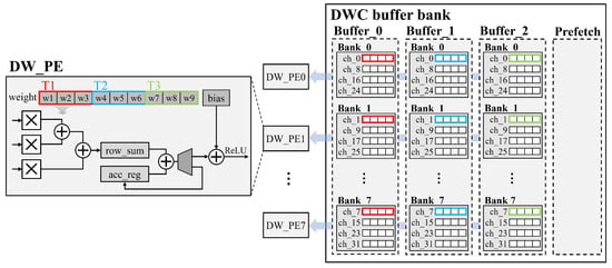
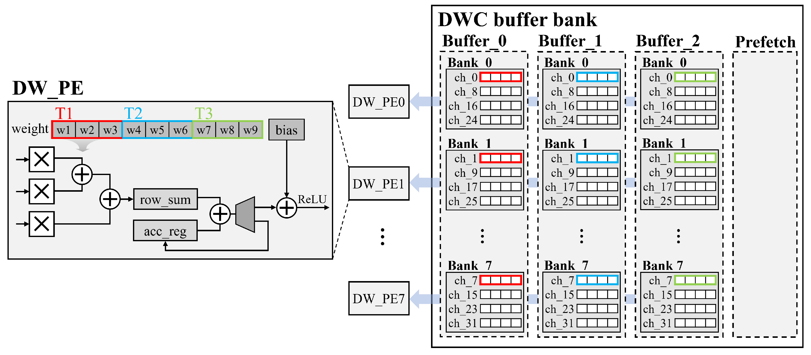
Figure 5 shows the structure of the modules constituting the DWC unit and the depthwise convolution process. The DWC unit consists of eight processing elements (DW PE), each comprising three multipliers and four adders. Since depthwise convolution is computed independently across channels, each DW PE is dedicated to a single channel, so that eight channels are processed in parallel. As every layer of MobileNetV1 has a channel count that is a multiple of 32, processing 32 channels at once is feasible; however, this would require supplying the input data of 32 channels simultaneously in each operation, requiring excessive buffer bandwidth. Taking this into account, the proposed design processes eight channels in parallel at a time. Furthermore, because the depthwise kernel is $3\times 3$, the three multipliers within each DW PE simultaneously compute the products of the three weights corresponding to one kernel row, yielding the partial sum of one row per clock cycle.

Figure 5. Architecture and operation flow of the DW PE in the DWC unit.

For example, suppose the input data are $112\times 112\times 32$ and rows 1, 2, and 3 are processed first. Then buffer 0, buffer 1, and buffer 2 store the data of rows 1, 2, and 3, respectively. Since eight channels are processed at a time, the 32 channels are divided into groups of eight and distributed across the banks: with respect to buffer 0, bank k holds the corresponding row data of channels k, $k+8$, $k+16$, and $k+24$. For instance, bank0 stores row 1 of channels 0, 8, 16, and 24, while bank7 stores row 1 of channels 7, 15, 23, and 31. Once the data of all three rows have been loaded, the depthwise convolution begins, and while the computation proceeds, the data of the next rows 4 and 5 are prefetched into the prefetch buffers.

The computation accumulates on a row-by-row basis. In Figure 5, during interval T1, the input and weights of the first row are read and multiplied, and their sum (row_sum) is added to the accumulation register (acc_reg). Since acc_reg is initialized to zero, the row-sum of the first row is stored directly. During T2, the row-sum of the second row is accumulated into acc_reg, and during T3, the third row is accumulated as well, yielding the sum of nine products, i.e., one output pixel. Adding the bias to the completed pixel and applying ReLU produces the final depthwise output; this process is carried out by eight channels in parallel, so that the outputs of eight channels at the same position are produced simultaneously. After the computation of rows 1, 2, and 3 for one group of eight channels is completed, the next eight channels are processed for rows 1, 2, and 3, and once all channels have been processed for rows 1, 2, and 3, the computation moves on to rows 2, 3, and 4. At this point, the buffer that previously held row 1 is loaded with the data of row 6, and the depthwise convolution over the entire feature map is performed sequentially in this manner.

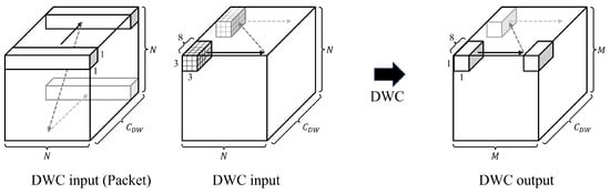
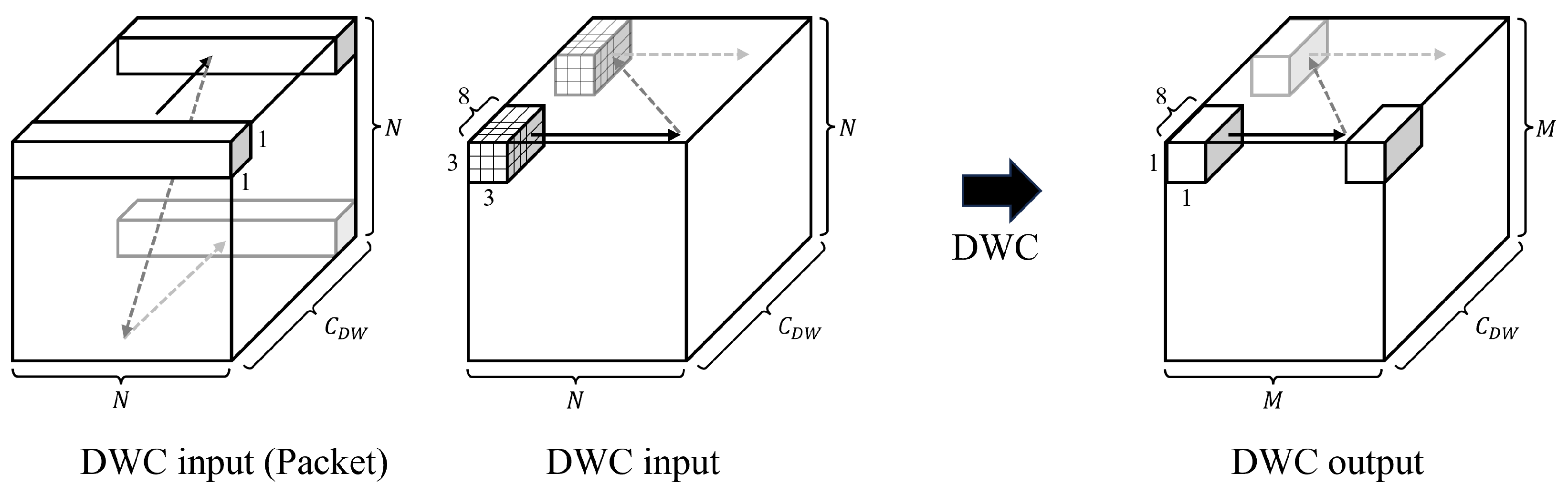
Figure 6 illustrates the data flow of the input and output during depthwise convolution. For an input feature map of size $N\times N\times C_{DW}$, one row of each channel is grouped in units of eight channels and transmitted to the DWC unit sequentially. Once all three rows required for the computation have been transmitted, the depthwise convolution begins. Since depthwise convolution preserves the number of channels, the output is of size $M\times M\times C_{DW}$; as shown on the right of Figure 6, the results of eight channels at a single output position ($1\times 1$) are generated sequentially along each row. While the buffers described above store input data only, the generated output is streamed directly into the PWC unit without being written to off-chip memory.

Figure 6. Data flow for Depthwise Convolution in the proposed hardware.

4.3. Pointwise Convolution Unit

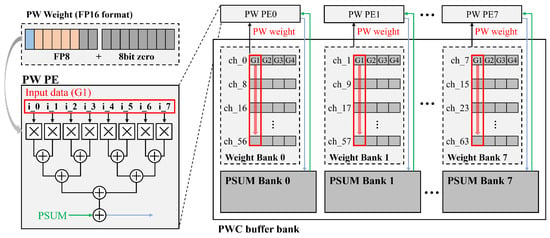
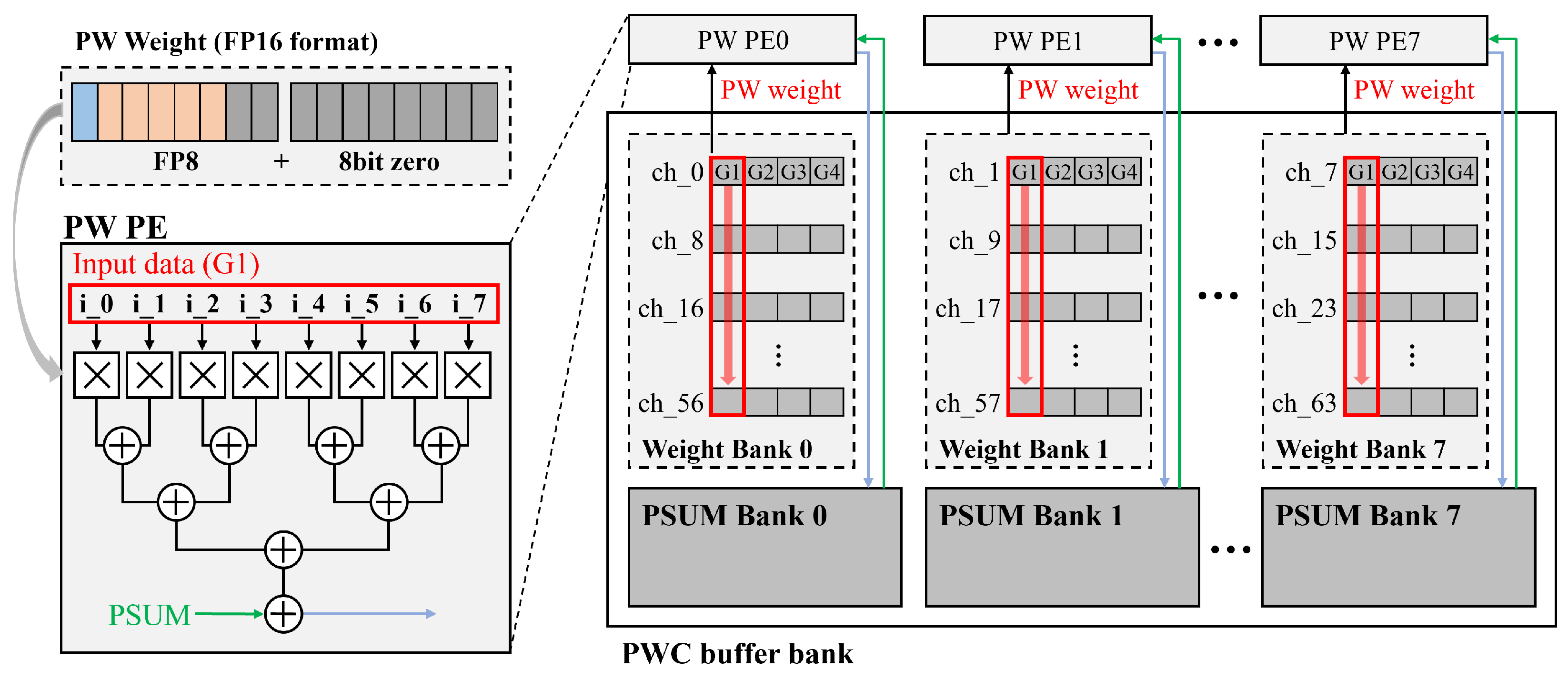
Figure 7 shows the structure of the modules constituting the PWC unit and the pointwise convolution process. The PWC unit likewise consists of eight processing elements (PW PE), each comprising eight multipliers and eight adders. The eight multipliers of each PW PE multiply eight input channels by the eight weights corresponding to one output channel, and the adders sum the results to produce the partial sum for that output channel. Since the pointwise weights are stored in FP8 (E5M2), each weight is expanded to FP16 at the input of its multiplier by appending eight zero bits. The multipliers of the PW PE therefore take FP16 operands. Unlike depthwise convolution, pointwise convolution combines the data of all input channels to generate a single output, and thus requires full inter-channel aggregation. However, since the DWC unit supplies its results in units of eight channels rather than all channels at once, the PWC unit performs the computation by dividing the input channels into groups of eight and accumulating partial sums. To this end, the PWC unit adopts an input-stationary scheme in which the input data are held fixed while the weights are swapped, in contrast to the DWC unit, which swaps its inputs. Accordingly, the PWC buffer bank assigns one weight bank and one PSUM bank to each PW PE, resulting in eight of each.

Figure 7. Architecture and operation flow of the PW PE in the PWC unit.

When the eight-channel result of the DWC unit is fed into the PWC unit, the same result is broadcast to all eight PW PEs. Each PW PE is responsible for a distinct set of output channels and sequentially processes a number of output channels equal to the total output channel count divided by eight. For example, when the pointwise weights are of shape $1\times 1\times 32$ with 64 output channels, each PW PE handles eight output channels. In this case, weight bank k stores the weights of output channels k, $k+8$, …, $k+56$; for instance, weight bank 0 stores the weights of output channels 0, 8, 16, …, 56, while weight bank 7 stores those of output channels 7, 15, 23, …, 63.

The computation proceeds in groups of output channels. When a DWC output is fed in, the eight PW PEs first compute output channels 0–7 simultaneously and store their partial sums in the PSUM banks, then compute output channels 8–15, and finally 56–63, storing each partial sum in the PSUM banks. After the partial sums for one group of eight input channels have been stored, the data of the next eight input channels at the same position are fed in, and the same computation is performed and accumulated with the partial sums already stored at the corresponding location in the PSUM banks. By repeating this process until the DWC result of the last eight input channels has been accumulated, the final sum of the output pixel is obtained. As in the DWC unit, the resulting PWC output is added with a bias and passed through ReLU to generate the final output.

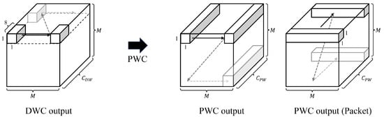
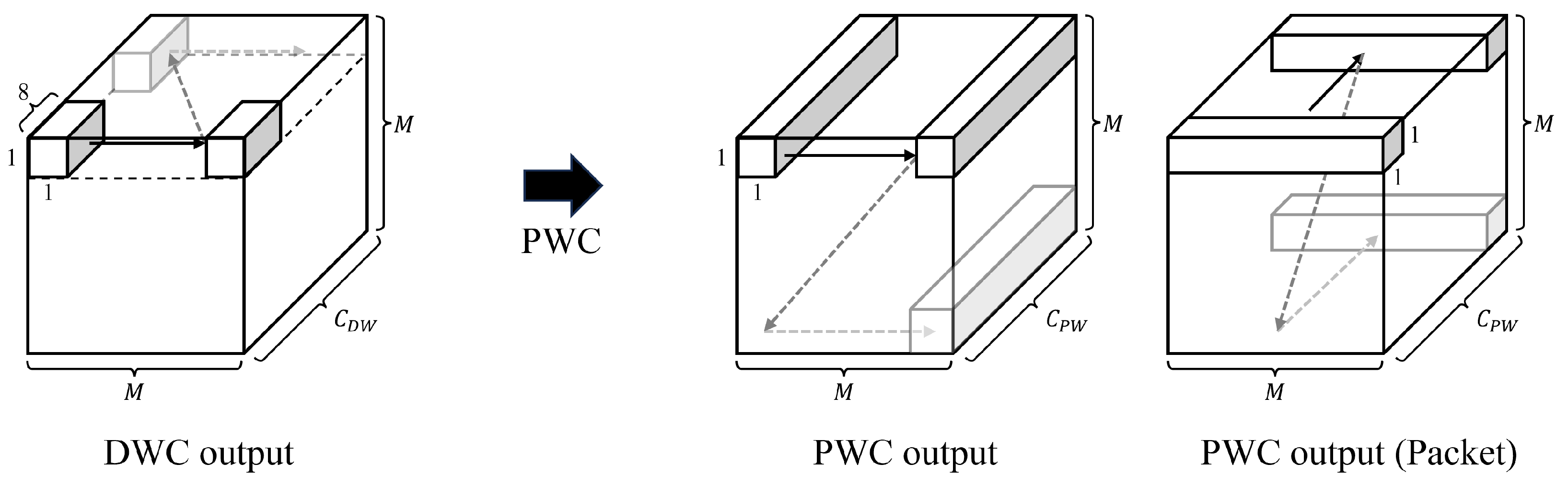
Figure 8 illustrates the data flow of the input and output during pointwise convolution. As the output of the DWC unit ($M\times M\times C_{DW}$) is fed in units of eight channels, partial-sum accumulation proceeds; once the data of all input channels for the first row have been processed, the results of the $C_{PW}$ output channels corresponding to the first row are produced sequentially, as shown in the middle of Figure 8. When the PWC results for one row are complete, they must be transmitted off-chip after RLC compression; to this end, the output is delivered to the RLC encoder module one row at a time per channel, as shown on the right of Figure 8.

Figure 8. Data flow for Pointwise Convolution in the proposed hardware.

5. Implementation and Experiments

This section presents experimental results to validate the two data-level techniques of the proposed architecture: RLC-based compression and mixed-precision quantization. We first analyze, through Python 3.10-based software simulations, the per-layer compression ratio achieved by the RLC algorithm and the changes in inference accuracy under various mixed-precision configurations. We then report the FPGA resource utilization of the hardware modules implemented in Verilog HDL and compare it with previous works.

5.1. Software Simulation

This subsection analyzes the per-layer RLC compression ratio and the inference accuracy under mixed-precision configurations, evaluated on MobileNetV1 pretrained on CIFAR-10, CIFAR-100 [29], and ImageNet [30].

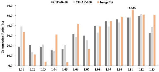
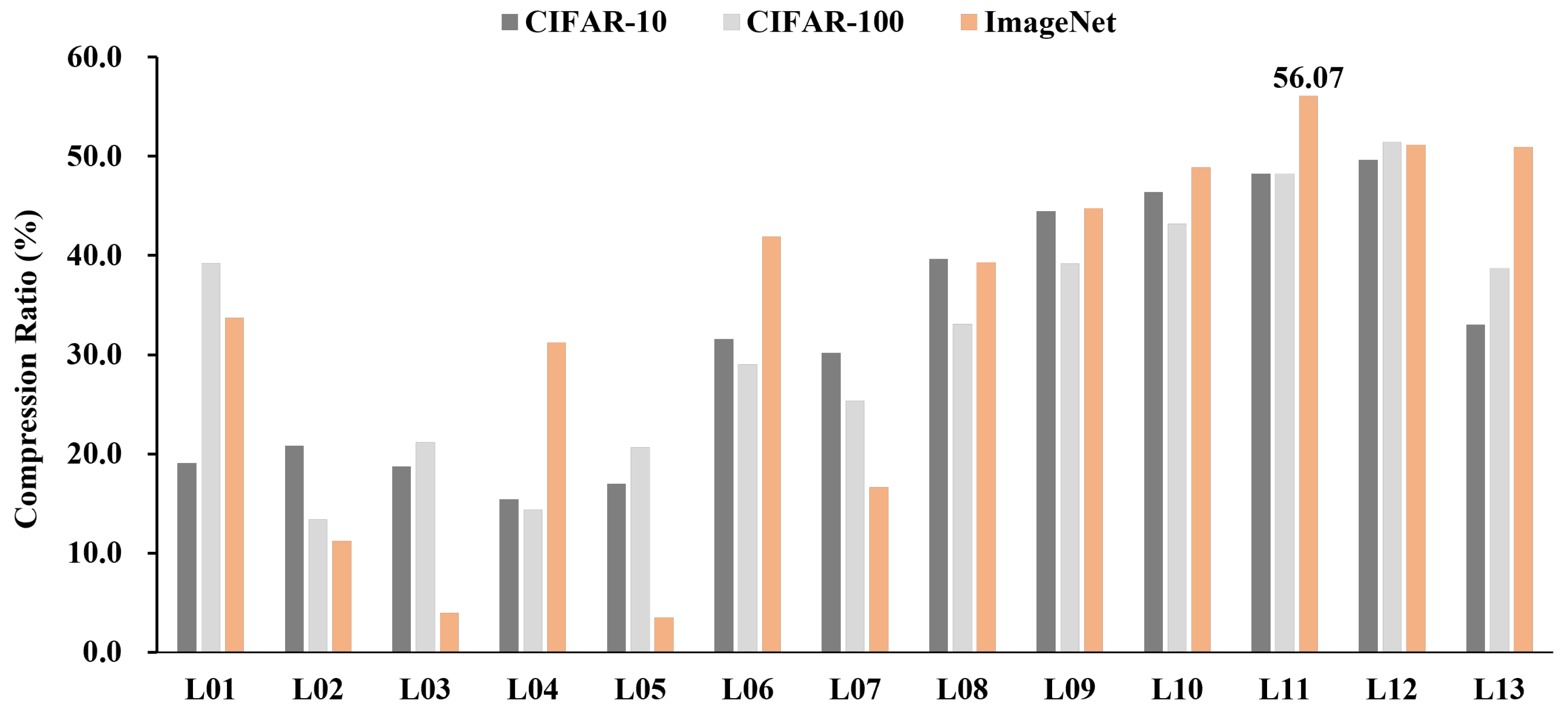
Figure 9 shows the per-layer compression ratio obtained when the RLC algorithm is applied to the input feature map of each layer of MobileNetV1. Although the compression ratio differs across datasets depending on their characteristics, it tends to increase as the layers deepen. As explained in Section 2.2, this is because the ReLU activation applied at each layer increases the proportion of zeros in the feature maps toward the later layers of the network. In the early layers, the low sparsity of the input feature map limits the compression efficiency, whereas the compression effect of the RLC algorithm becomes markedly more pronounced in the deeper layers. In particular, on ImageNet, Layer 11 achieves a maximum compression ratio of 56.07%, confirming that the RLC algorithm effectively contributes to reducing the transmission bandwidth in the deeper layers. As shown in Figure 9, Layers 3 and 5 on ImageNet show the smallest compression ratios, 3.96% and 3.48%, because the proportion of zeros in these layers is close to the break-even point of the packet format. The compression ratio nevertheless remains positive in every layer of all three datasets, so the RLC does not increase the amount of data transferred in any of the evaluated layers.

Figure 9. RLC Compression Ratio of Input Data per Layer in MobileNetV1. Each value is averaged over 1000 test images per dataset.

Table 1 reports the Top-1 accuracy obtained under different mixed-precision configurations of the parameters. The MobileNetV1 models were trained in full precision (FP32), and the mixed-precision quantization was applied as a post-training step without quantization-aware retraining or fine-tuning. In all experiments, the feature maps are fixed to FP16, and four configurations are evaluated by setting the DW and PW parameters to either FP16 or FP8 (E5M2). Among the four configurations, converting all parameters to FP8 results in the largest accuracy degradation across all three datasets, with an 18.99 percentage point (pp) drop on ImageNet in particular, confirming that uniform low-precision quantization is unsuitable. We therefore analyzed the precision sensitivity separately for each operation type. Applying FP8 only to the PW parameters incurs accuracy losses of 0.22 pp, 0.80 pp, and 6.24 pp on CIFAR-10, CIFAR-100, and ImageNet, respectively, whereas applying FP8 only to the DW parameters results in losses of 0.38 pp, 1.74 pp, and 15.98 pp. These results confirm that the depthwise convolution is more sensitive to precision reduction than the pointwise convolution. This is because the DW operation is directly responsible for spatial feature extraction and is thus sensitive to precision reduction, whereas the PW operation, which primarily performs channel-wise combination, maintains relatively stable outputs even at lower precision [31,32].

Table 1. Top-1 accuracy (%) and accuracy drop in percentage points (pp) relative to the all-FP16 baseline under different mixed-precision configurations. The first row is the unquantized FP32 model, in which the feature maps are also in FP32; it differs from the all-FP16 baseline by at most 0.02 pp in either direction.

Precision		CIFAR-10		CIFAR-100		ImageNet
DW	PW	Top-1	Drop ↓	Top-1	Drop ↓	Top-1	Drop ↓
FP32	FP32	94.64	—	76.57	—	69.79	—
FP16	FP16	94.62	0.00	76.56	0.00	69.80	0.00
FP16	FP8	94.40	0.22	75.76	0.80	63.56	6.24
FP8	FP16	94.24	0.38	74.82	1.74	53.82	15.98
FP8	FP8	94.13	0.49	74.13	2.43	50.80	18.99

Table 2 presents the parameter storage and the corresponding reduction for the four mixed-precision configurations. In the entire MobileNetV1 model, the PW parameters account for the vast majority of all parameters. Accordingly, applying FP8 to the PW parameters achieves a 49.22% reduction in storage, whereas applying it only to the DW parameters yields only 0.78%. Based on these results, we selected the mixed-precision configuration that keeps the DW weights and biases in FP16 while converting the PW weights and biases to FP8 (E5M2). Among the four evaluated configurations, this combination is the hardware-compatible trade-off that minimizes inference accuracy loss while maximizing the reduction in parameter storage. This configuration was adopted in the actual hardware design.

Table 2. Parameter storage of the depthwise convolution and pointwise convolution layers and the resulting storage reduction relative to the all-FP16 baseline under different mixed-precision configurations.

Precision		Memory Usage (KB)		Saving (%)
DW	PW	DW	PW
FP16	FP16	96.88	6143.63	0.00
FP16	FP8	96.88	3071.81	49.22
FP8	FP16	48.44	6143.63	0.78
FP8	FP8	48.44	3071.81	50.00

5.2. Hardware Implementation Results

The proposed hardware is an accelerator for depthwise separable convolution, designed in Verilog HDL and synthesized and implemented for a Xilinx Zynq UltraScale+ ZCU-104 board (XCZU7EV-2FFVC1156) using the Xilinx Vivado 2025.1 environment. Rather than being tied to a specific layer, the proposed circuit is designed to process all depthwise separable convolution layers of MobileNetV1 with a single engine, according to the layer parameters delivered by an instruction. Functional verification was performed on a per-layer basis for each depthwise separable convolution layer, and the hardware output was confirmed to be bit-accurate with the mixed-precision (FP16/FP8) software golden results for the same inputs. The power result reported in this paper is the total on-chip power obtained from the Vivado implementation report for the design implemented at 150 MHz.

Because the RLC decoder in the proposed design emits a variable number of elements per cycle while the DWC unit consumes eight channels per cycle, we first measured whether the decoder keeps the DWC unit supplied, using counters that do not affect the design under test. The proposed accelerator was compared with the same accelerator without RLC, in which the feature map is transferred uncompressed, four FP16 elements per 64-bit word, with every row of a channel starting at a word boundary; the two versions are identical in every other respect and produce the same outputs. Table 3 shows the decoder output rate and the stall ratio of the DWC unit for each layer. The proposed decoder produces 3.83 to 5.13 elements per cycle, against 3.50 to 4.00 without RLC, because a 64-bit word holds four elements and the last word of a row may be only partly filled, whereas a single packet can expand a run of zeros into more than four. The decoder is active for at most 14.0% of the cycles in which the DWC unit is running, so it supplies data and then remains idle for most of the execution; the decoder itself is therefore unlikely to be the dominant source of stall. The stall ratio of the DWC unit is lower with RLC in every layer, by 1.5 to 57.2 percentage points, so RLC never increases this stall relative to uncompressed transfer, and in the layers where the ratio remains high with RLC it is comparably high without RLC as well, indicating that the shared host interface, rather than the decoder, limits supply in those layers.

Table 3. Per-layer comparison of the accelerator with and without RLC (RTL simulation, one CIFAR-100 input). Stall ratio is the fraction of running cycles with an incomplete prefetch buffer; traffic is feature-map bytes exchanged with the host per layer.

Layer	Output Rate RLC/No RLC	Decoder Occupancy (%)	Stall Ratio (%)	Traffic (KB) RLC/No RLC	Reduction (%)
1	4.56/4.00	14.0	4.2/61.4	1854.4/2352.0	21.2
2	3.86/4.00	5.5	84.3/86.4	2012.8/2352.0	14.4
3	4.02/4.00	6.3	46.9/57.5	1357.6/1568.0	13.4
4	3.84/4.00	5.3	79.8/81.7	1067.9/1176.0	9.2
5	3.95/4.00	5.6	12.6/21.2	668.7/784.0	14.7
6	4.30/4.00	5.5	56.6/65.0	504.0/616.0	18.2
7	3.83/3.50	3.2	10.5/12.0	357.5/448.0	20.2
8	4.24/3.50	3.0	9.0/12.0	322.3/448.0	28.1
9	4.45/3.50	2.8	8.9/12.0	301.3/448.0	32.7
10	4.60/3.50	2.8	8.4/12.0	272.9/448.0	39.1
11	4.92/3.50	2.6	7.4/12.0	243.6/448.0	45.6
12	5.13/3.50	5.5	14.3/46.8	199.3/336.0	40.7
13	4.73/3.50	1.6	10.9/14.0	180.4/224.0	19.5

For this representative input, the same comparison also gives the amount of data exchanged with the host. Over the 13 layers the proposed design transfers 9,566,848 bytes of activation data, against 11,927,552 bytes without RLC, a reduction of 19.8%, with the per-layer reduction ranging from 9.2% to 45.6% (Table 3). This reduction follows directly from the packet-level RLC compression ratio, which Figure 9 shows to be consistent across 1000 test images per dataset in software. The single input used for the RTL simulation is therefore representative rather than an outlier. The weight traffic is identical in the two designs because only the activations are compressed. Summing these per-layer figures, the same interface is expected to carry the activation data of one inference about 1.25 times faster, with the delay from the first input byte to the first output about 8.5% to 34.6% shorter. Adding the encoder and the decoder increases the LUT usage by only 0.90% and the flip-flop usage by 2.58%, and requires no additional block RAM, UltraRAM or DSP (Table 4). RLC therefore reduces the data exchanged with the host without increasing the on-chip memory.

Table 4. FPGA resource utilization of the proposed accelerator. The baseline is the same accelerator with the RLC encoder and decoder replaced by fixed-length packing.

	LUT	FF	BRAM	URAM	DSP
Total	230,400	460,800	312	96	1728
Utilization (proposed)	79,457	8957	101	32	88
Utilization (baseline)	78,749	8732	101	32	88
Usage rate (proposed)	34.5%	1.9%	32.4%	33.3%	5.1%

Table 4 shows the resource utilization of the proposed accelerator on the target FPGA board. The design uses 79,457 LUTs (approximately 34.5% of the total), 8957 FFs (approximately 1.9%), 101 BRAMs (approximately 32.4%), and 88 DSPs (approximately 5.1%). The FF utilization, in particular, is remarkably low at 1.9%, because the feature maps and weights are explicitly mapped to dedicated on-chip memories, thereby suppressing excessive flip-flop usage. The BRAM utilization is likewise kept at 32.4% because the decoded feature map is buffered one row at a time rather than in its entirety, and because the depth of each on-chip memory is sized to the maximum required across layers.

The 32 URAMs (33.3%) are dedicated to on-chip storage of the pointwise convolution weights, eliminating off-chip parameter accesses and enabling low-latency weight retrieval throughout inference. This weight memory is sized to the largest pointwise layer, and storing the weights in FP8 rather than FP16 halves its width, so it is implemented with 32 URAMs instead of 64. The FP8 format therefore halves the on-chip weight storage without changing the multiplier array. The DSPs implement the FP16 multipliers of the two engines, 24 in the DWC unit and 64 in the PWC unit. Since the pointwise weights are expanded to FP16 before the multiplier array, both engines use the same FP16 multiplier, and only 88 DSPs are required in total, which is 5.1% of all DSPs. As most of the resource utilization is kept below 35%, the design retains ample headroom to further scale the computational parallelism or to accommodate larger models on the same board.

Table 5 compares the proposed accelerator, in terms of resource utilization, with previous FPGA-based depthwise separable convolution accelerators for MobileNet-family models. The proposed design employs a mixed-precision scheme that processes the feature maps in FP16 and the pointwise weights in FP8 (E5M2). It uses only 79.5k LUTs, fewer than the prior works [13,23,33], and its FF count of 9.0k is only about $1/14$ to $1/31$ of those reported in the prior works. This is a result of adopting explicit on-chip memory mapping instead of register-based buffers, which substantially reduces flip-flop usage. The proposed design also exhibits a smaller memory footprint than prior works, mainly because the pointwise weights are stored in FP8. In addition, a streaming architecture that begins computation as soon as the required data are ready reduces the size of the intermediate buffers, so the buffers hold only the rows required by the DWC unit rather than a complete feature map. In contrast, the throughput is lower than that of the prior designs, since the primary objective of the proposed design is to minimize on-chip memory usage rather than to maximize processing speed. In summary, the proposed accelerator performs MobileNetV1 inference with minimal on-chip memory and logic, making it well suited to resource-constrained edge devices.

Table 5. Comparison of resource utilization with previous works.

	[13]	[33]	[23]	Proposed
Model	MobileNetV2	MobileNetV1	MobileNetV1	MobileNetV1
Platform	Xilinx XC7V690T	Xilinx XC7Z045	Xilinx XCZU9EG	Xilinx XCZU7EV
Data Format	INT8	Fixed-8	Fixed-8	Mixed (FP16/FP8)
Clock (MHz)	150	150	150	150
LUT/FF (k)	308.4/278.9	154/128	214.9/166.7	79.5/9.0
DSP Usage	2160	787	69	88
Memory Usage (Mb)	33.10	18.88	17.81	12.55
GOPS	181.8	13.0	108.3	-
GFLOPS	-	-	-	26.40
Power (W)	11.35	6.24	5.95	1.53
GOPS/W	16.02	2.08	18.20	-
GFLOPS/W	-	-	-	17.25

6. Conclusions

In this paper, we proposed a memory-efficient hardware accelerator for the depthwise separable convolution of MobileNetV1, aiming to minimize off-chip memory traffic and parameter storage. The proposed architecture consists of a 64-bit RLC packet compression that exploits the sparsity of feature maps after ReLU, a mixed-precision scheme that applies different precisions to the parameters, and a streaming compute structure in which the depthwise and pointwise convolutions are separated and connected in a pipeline. By transmitting feature maps in compressed form and decoding them row by row, the architecture keeps only the rows required for computation in the on-chip buffers. Software simulation showed that the RLC compression ratio increases with network depth, reaching up to 56.07% on ImageNet, while the mixed-precision configuration reduced parameter storage by 49.22% at a cost of 6.24 pp in Top-1 accuracy. We implemented the proposed accelerator in Verilog HDL on a Xilinx ZCU-104 FPGA. It performs depthwise separable convolution using only a small amount of logic resources and on-chip memory. Future work will focus on improving the throughput by increasing the computational parallelism and operating frequency while preserving memory efficiency, as well as integrating the design at the full-network level and extending it to a wider range of models. The 6.24 pp accuracy loss on ImageNet also remains to be addressed, through quantization-aware fine-tuning and through an integer datapath in which INT8 can be reconsidered.

References

- Kim, R.; Park, J.; Kim, J.; Oh, J.; Lee, S.E. Real-Time True Wireless Stereo Wearing Detection Using a PPG Sensor with Edge AI. Electronics 2025, 14, 3911. [Google Scholar] [CrossRef] [Scilit]
- Park, J.; Shin, J.; Kim, R.; An, S.; Lee, S.; Kim, J.; Oh, J.; Jeong, Y.; Kim, S.; Jeong, Y.R.; et al. Accelerating strawberry ripeness classification using a convolution-based feature extractor along with an edge AI processor. Electronics 2024, 13, 344. [Google Scholar] [CrossRef] [Scilit]
- Liu, L.; Zhao, M.; Yu, M.; Jan, M.A.; Lan, D.; Taherkordi, A. Mobility-aware multi-hop task offloading for autonomous driving in vehicular edge computing and networks. IEEE Trans. Intell. Transp. Syst. 2022, 24, 2169–2182. [Google Scholar] [CrossRef] [Scilit]
- Shin, J.; Park, J.; Kim, J.; Jeong, Y.R.; An, S.; Lee, S.E. An Accelerated Block Searching Approach in A* for Autonomous Mobile Robots. In Proceedings of the IEEE Transactions on Circuits and Systems I: Regular Papers; IEEE: New York, NY, USA, 2025. [Google Scholar]
- Jeong, Y.W.; Oh, H.W.; Jang, S.Y.; Lee, S.E. Intelligent Transportation System based on an Edge AI. In Proceedings of the International Conference on Future Information & Communication Engineering, Jeju Island, Republic of Korea, 12–14 January 2022; pp. 202–206. [Google Scholar]
- Lamdjad, B. Edge AI-driven adaptive maintenance for manufacturing systems: Improving decision-making and reducing energy consumption. J. Intell. Manuf. Spec. Equip. 2025, 6, 312–326. [Google Scholar] [CrossRef] [Scilit]
- Kim, S.; Park, J.; Jeong, Y.; Lee, S.E. Embedded monitoring system for preventing lonely death based on edge AI. In Proceedings of the 2023 IEEE International Conference on Consumer Electronics (ICCE); IEEE: New York, NY, USA, 2023; pp. 1–2. [Google Scholar]
- Rosa, M.; Burget, R.; Hubálek, J. Energy-efficient activity and sleep recognition using edge computing and wearable devices. In Proceedings of the 2025 17th International Congress on Ultra Modern Telecommunications and Control Systems and Workshops (ICUMT); IEEE: New York, NY, USA, 2025; pp. 211–217. [Google Scholar]
- Younesi, A.; Ansari, M.; Fazli, M.; Ejlali, A.; Shafique, M.; Henkel, J. A comprehensive survey of convolutions in deep learning: Applications, challenges, and future trends. IEEE Access 2024, 12, 41180–41218. [Google Scholar] [CrossRef] [Scilit]
- Howard, A.G.; Zhu, M.; Chen, B.; Kalenichenko, D.; Wang, W.; Weyand, T.; Andreetto, M.; Adam, H. Mobilenets: Efficient convolutional neural networks for mobile vision applications. arXiv 2017, arXiv:1704.04861. [Google Scholar]
- Zhang, X.; Yang, J. A High Performance FPGA-based Accelerator for MobileNet. In Proceedings of the 2022 International Conference on Informatics, Networking and Computing (ICINC); IEEE: New York, NY, USA, 2022; pp. 81–85. [Google Scholar]
- Srivastava, H.; Sarawadekar, K. A depthwise separable convolution architecture for CNN accelerator. In Proceedings of the 2020 IEEE Applied Signal Processing Conference (ASPCON); IEEE: New York, NY, USA, 2020; pp. 1–5. [Google Scholar]
- Yan, S.; Liu, Z.; Wang, Y.; Zeng, C.; Liu, Q.; Cheng, B.; Cheung, R.C. An FPGA-based MobileNet accelerator considering network structure characteristics. In Proceedings of the 2021 31st International Conference on Field-Programmable Logic and Applications (FPL); IEEE: New York, NY, USA, 2021; pp. 17–23. [Google Scholar]
- Liao, J.; Cai, L.; Xu, Y.; He, M. Design of accelerator for MobileNet convolutional neural network based on FPGA. In Proceedings of the 2019 IEEE 4th Advanced Information Technology, Electronic and Automation Control Conference (IAEAC); IEEE: New York, NY, USA, 2019; Volume 1, pp. 1392–1396. [Google Scholar]
- Huang, J.; Liu, X.; Guo, T.; Zhao, Z. A high-performance FPGA-based depthwise separable convolution accelerator. Electronics 2023, 12, 1571. [Google Scholar] [CrossRef] [Scilit]
- Huang, Z.; Qie, A.; Zhang, C.; Yang, J.; Wang, X. Exploration for efficient depthwise separable convolution networks deployment on FPGA. In Proceedings of the 2024 IEEE 6th International Conference on AI Circuits and Systems (AICAS); IEEE: New York, NY, USA, 2024; pp. 213–217. [Google Scholar]
- Kang, D.; Kang, D.; Ha, S. Multi-bank on-chip memory management techniques for CNN accelerators. IEEE Trans. Comput. 2021, 71, 1181–1193. [Google Scholar] [CrossRef] [Scilit]
- Simonyan, K.; Zisserman, A. Very deep convolutional networks for large-scale image recognition. arXiv 2014, arXiv:1409.1556. [Google Scholar]
- He, K.; Zhang, X.; Ren, S.; Sun, J. Deep residual learning for image recognition. In Proceedings of the IEEE Conference on Computer Vision and Pattern Recognition, Las Vegas, NV, USA, 27–30 June 2016; pp. 770–778. [Google Scholar]
- Golomb, S. Run-length encodings (corresp.). IEEE Trans. Inf. Theory 1966, 12, 399–401. [Google Scholar] [CrossRef] [Scilit]
- Micikevicius, P.; Narang, S.; Alben, J.; Diamos, G.; Elsen, E.; Garcia, D.; Ginsburg, B.; Houston, M.; Kuchaiev, O.; Venkatesh, G.; et al. Mixed precision training. arXiv 2017, arXiv:1710.03740. [Google Scholar]
- Lee, J.; Lee, J.; Han, D.; Lee, J.; Park, G.; Yoo, H.J. An energy-efficient sparse deep-neural-network learning accelerator with fine-grained mixed precision of FP8–FP16. IEEE Solid-State Circuits Lett. 2019, 2, 232–235. [Google Scholar] [CrossRef] [Scilit]
- Hong, H.; Choi, D.; Kim, N.; Kim, H. Mobile-X: Dedicated FPGA implementation of the MobileNet accelerator optimizing depthwise separable convolution. IEEE Trans. Circuits Syst. II Express Briefs 2024, 71, 4668–4672. [Google Scholar] [CrossRef] [Scilit]
- Wu, D.; Zhang, Y.; Jia, X.; Tian, L.; Li, T.; Sui, L.; Xie, D.; Shan, Y. A high-performance CNN processor based on FPGA for MobileNets. In Proceedings of the 2019 29th International Conference on Field Programmable Logic and Applications (FPL); IEEE: New York, NY, USA, 2019; pp. 136–143. [Google Scholar]
- Ou, J.; Li, X.; Sun, Y.; Shi, Y. A configurable hardware accelerator based on hybrid dataflow for depthwise separable convolution. In Proceedings of the 2022 4th International Conference on Advances in Computer Technology, Information Science and Communications (CTISC); IEEE: New York, NY, USA, 2022; pp. 1–5. [Google Scholar]
- Sang, X.; Ruan, T.; Li, C.; Li, H.; Yang, R.; Liu, Z. A real-time and high-performance MobileNet accelerator based on adaptive dataflow scheduling for image classification. J. Real.-Time Image Process. 2024, 21, 4. [Google Scholar] [CrossRef] [Scilit]
- Lin, Y.; Zhang, Y.; Yang, X. A low memory requirement mobilenets accelerator based on FPGA for auxiliary medical tasks. Bioengineering 2022, 10, 28. [Google Scholar] [CrossRef] [Scilit] [PubMed]
- Xuan, L.; Un, K.F.; Lam, C.S.; Martins, R.P. An FPGA-based energy-efficient reconfigurable depthwise separable convolution accelerator for image recognition. IEEE Trans. Circuits Syst. II Express Briefs 2022, 69, 4003–4007. [Google Scholar] [CrossRef] [Scilit]
- Krizhevsky, A.; Hinton, G. Learning multiple layers of features from tiny images. In Technical Report; University of Toronto: Toronto, ON, Canada, 2009. [Google Scholar]
- Deng, J.; Dong, W.; Socher, R.; Li, L.J.; Li, K.; Fei-Fei, L. Imagenet: A large-scale hierarchical image database. In Proceedings of the 2009 IEEE Conference on Computer Vision and Pattern Recognition; IEEE: New York, NY, USA, 2009; pp. 248–255. [Google Scholar]
- Yun, S.; Wong, A. Do all mobilenets quantize poorly? gaining insights into the effect of quantization on depthwise separable convolutional networks through the eyes of multi-scale distributional dynamics. In Proceedings of the IEEE/CVF Conference on Computer Vision and Pattern Recognition, Virtual, 20–25 June 2021; pp. 2447–2456. [Google Scholar]
- Sheng, T.; Feng, C.; Zhuo, S.; Zhang, X.; Shen, L.; Aleksic, M. A quantization-friendly separable convolution for mobilenets. arXiv 2018, arXiv:1803.08607. [Google Scholar]
- Liu, W.; Li, Y.; Yang, Y.; Zhu, J.; Liu, L. Design an efficient DNN inference framework with PS-PL synergies in FPGA for edge computing. In Proceedings of the 2022 China Automation Congress (CAC); IEEE: New York, NY, USA, 2022; pp. 4186–4190. [Google Scholar]
Disclaimer/Publisher’s Note: The statements, opinions and data contained in all publications are solely those of the individual author(s) and contributor(s) and not of MDPI and/or the editor(s). MDPI and/or the editor(s) disclaim responsibility for any injury to people or property resulting from any ideas, methods, instructions or products referred to in the content. |
© 2026 by the authors. Licensee MDPI, Basel, Switzerland. This article is an open access article distributed under the terms and conditions of the Creative Commons Attribution (CC BY) license.