Revisiting Differentially Private Federated Learning for Tabular Data: A Matched-Accounting Benchmark of Boosting Versus DP-SGD

Abstract

Gradient-boosted trees outperform neural networks on tabular data without privacy, often taken to imply that differentially private federated learning should be based on boosting. We revisit this implication under matched accounting—a single privacy-loss distribution accountant, cross-checked against Rényi accounting—and symmetric, per-budget tuning, and find limited support for this expectation. On the Diabetes 130-US-Hospitals and BRFSS datasets across ε ∈ {0.5, 1, 2, 4, 8} over 20 seeds, differentially private federated boosting, a differentially private stochastic gradient descent (DP-SGD) network, and DP-SGD logistic regression achieve similar performance; no model class is consistently superior. On the real corpora, the most frugal model wins at the tightest budget—logistic regression is best at ε = 0.5 (0.589 and 0.811 AUC)—while the network leads slightly at looser budgets; boosting remains competitive but does not lead. On the synthetic task, boosting leads at tight budgets and the network at looser ones. The comparison is asymmetrically tuning-sensitive: fixing the boosting round count can produce an apparent neural advantage, whereas the network is robust to its step count. Off-path privatization and sequential noise accumulation explain the behavior; boosting’s main advantage is not accuracy but communication, achieving one to three orders of magnitude fewer values per client.

1. Introduction

Two well-supported facts make differentially private (DP) federated boosting appear to be a natural design choice for clinical tabular data—and frame the question that this article answers. First, on tabular problems, gradient-boosted trees routinely beat neural networks of comparable engineering effort: they discard uninformative features, tolerate irregular decision boundaries, and ignore feature scaling [1,2]. Second, hospital records cannot be pooled, so federated learning under formal privacy guarantees often becomes a central operating constraint [3,4]. Together, these facts motivate the use of differentially private federated boosting [5,6].

Our results do not fully support this premise under matched accounting and fair tuning. Boosting does not retain a consistent accuracy advantage under privacy, and neural networks do not show a consistent advantage either. The three model classes achieve similar performance, and the leading method depends more on the dataset and privacy budget than on the model class alone. Across the two real corpora, the most frugal model, logistic regression, wins at the tightest budget, while boosting leads only where the task is genuinely nonlinear. The apparent neural advantage a comparison with fixed boosting rounds may report is largely explained by a correctable tuning choice—holding the boosting round count fixed across budgets—so model class choice appears less decisive for accuracy than expected; communication cost becomes a more informative basis for choosing among them.

Two methodological issues motivate the analysis. The first is off-path privatization: applying differential privacy to a quantity that never enters the predictor, such as a feature importance vector used only for interpretation, leaves predictions unchanged and therefore does not protect the prediction path. The second is asymmetric tuning: comparing a carefully tuned method against a baseline whose privacy-sensitive hyperparameters are not retuned across budgets.

We organize this study around three research questions.

RQ1. 

Does the non-private tabular advantage of gradient boosting survive differential privacy in the federated setting?

RQ2. 

Are the reported advantages of private federated boosting—or of neural alternatives—robust to a single matched accountant and symmetric, per-budget hyperparameter tuning?

RQ3. 

What mechanism explains the privacy–utility behavior of DP boosting relative to DP-SGD (differentially private stochastic gradient descent), and why is the comparison so tuning-sensitive?

Our contributions are as follows:

• We formalize and demonstrate the off-path privatization pitfall (Lemma 1): noise on interpretation metadata yields budget-invariant accuracy and does not protect the prediction path, so a flat privacy–utility curve indicates that the prediction path is not protected, rather than providing evidence of model-level privacy.
• We provide a fair, matched-accounting benchmark of DP federated boosting, DP-SGD networks, and DP-SGD logistic regression on synthetic data and two real tabular health corpora, across five privacy budgets, with 20 seeds and both paired and rank-based significance tests. No model class dominates; differences are small and budget- and dataset-dependent.
• We show the comparison is sensitive to asymmetric tuning: the boosting round count is the sensitive hyperparameter—holding it fixed across budgets produces an apparent neural advantage—whereas the DP-SGD network is robust to its step count and is hurt, not helped, by added width.
• We give a mechanistic account, formalized as Proposition 1 and confirmed empirically: boosting accumulates per-round noise through sequential dependence and often reaches its optimum at relatively few rounds under privacy, whereas DP-SGD averages independent per-step noise and is robust to the step count.
• We define a single, matched-accounting evaluation protocol—one accountant, symmetric per-budget tuning, and 20-seed significance testing—that makes private tabular comparisons reproducible and directly comparable.

2. Related Work and Positioning

Differential privacy and DP-SGD. Differential privacy limits how much any single record can move a released computation [7,8]. DP-SGD carries this into iterative training by clipping per-example gradients and adding calibrated Gaussian noise [9]; subsampling amplification then lets many noisy steps compose to a modest total budget. This composition is tracked tightly using the moments accountant and Rényi differential privacy (RDP) [10,11,12], with f-/Gaussian DP [13], and most sharply with numerical privacy-loss distribution (PLD) methods [14,15]—our reference accountant. Two modeling choices fix our setting: the central model with trusted aggregation rather than the stricter local model, and record-level rather than user- or client-level granularity, since client-level DP in federated learning is a distinct and stricter regime [16] and user-level DP has been studied mainly in large-scale sequence models [16]. Hybrid schemes that fuse cryptographic with statistical protection are orthogonal to the matched-accounting question pursued here [17].

Private and federated tree ensembles. Differentially private tree learning is now a broad research area: private decision-tree induction [18], random decision trees [19], private random forests via smooth sensitivity [20], and private gradient boosting that privatizes split selection and leaf statistics [5,21], with histogram mechanisms noising per-leaf gradient and Hessian sums. Federated variants add cross-party coordination: SecureBoost under cryptographic protection [6], a guarantee orthogonal to DP; federated gradient-boosted decision tree (GBDT) systems [22] and FederBoost [23] across horizontal and vertical partitions; and, most directly, federated boosting composed with differential privacy [24]. Less commonly addressed is benchmarking against a fairly tuned DP-SGD baseline under an identical accountant; comparisons pit boosting against other boosting, or against non-private references. However, private empirical risk minimization theory [25,26] and the broader DP learning toolkit [27,28,29] make gradient-based private learners strong, well-understood competitors. This article addresses that gap.

Trees versus deep learning on tabular data. Careful non-private benchmarks still favor tree ensembles over deep networks on typical tabular problems [1,2], and surveys [30] together with tabular-specific architectures—revisited deep models [31] and attention designs such as TabNet [32]—show how sharply neural performance on tabular data depends on representation, tuning, and dataset structure. These results, however, are obtained in non-private settings; the ranking changes once privacy constraints are imposed. The properties that make trees strong in the clear do not necessarily make them preferable under privacy-induced noise, and the private regime does not transfer the advantage to neural networks either.

Why the gap matters: privacy attacks and benchmarking. An incomplete comparison can lead to misleading conclusions: models without prediction-path noise leak their training data to membership inference and reconstruction attacks [33,34,35], so a flat privacy–utility curve from off-path noise (Section 5.1) is a potentially unprotected prediction path, not evidence of a favorable privacy–utility trade-off. The benchmarking literature likewise shows that empirical verdicts hinge on evaluation choices—careful baselines and tuning for private learning [36,37,38], standardized reproducible protocols for federated-healthcare benchmarks [39,40,41]. The matched-accounting, symmetric-tuning design used here addresses both concerns.

Table 1 places representative prior work along the axes that decide whether a private tree-versus-network claim is sound. The characterizations reflect how each line of work is typically reported; the comparison is intended to summarize methodological coverage rather than evaluate individual studies.

Table 1. Positioning against representative private learning and federated-boosting work.

Method	Federated	Accountant	Fair Neural Baseline	Health Data
DP-SGD (network) [9]	—	moments/RDP	is the network	image/text
DP decision tree [18]	—	composition	no	no
DP random forest [20]	—	smooth sens.	no	some
DP-GBDT [5]	—	composition	no	no
SecureBoost [6]	vertical	crypto (not DP)	no	varies
Federated GBDT [22,23]	horiz./vert.	crypto/DP	no	no
DP federated boosting [24]	horizontal	RDP	partial	no
FLamby (neural benchmark) [41]	cross-silo	varies	n/a	yes
This work: boosting + DP-SGD + DP-logistic (ours)	horizontal	PLD (RDP-checked)	yes (per-ε)	yes (two)

Table 2 distills those recurring methodological issues into the safeguards a sound private-tabular comparison requires, set against prevailing practice and the protocol adopted here.

Table 2. Methodological safeguards used in this benchmark.

Safeguard	Common Practice	This Benchmark
DP noise on the prediction path	Sometimes off-path	Always on-path
Single accountant for all methods	Often mixed/unstated	One PLD accountant (RDP-checked)
Symmetric, per-budget tuning of baselines	Frequently asymmetric	Both sides, per budget
Tree + neural + linear baselines	Usually one family	All three
Multiple privacy budgets	Often a single ε	ε ∈ {0.5,1,2,4,8}
Real tabular-health data	Variable	Two real corpora + synthetic
Paired & rank-based tests	Rare	Yes (20 seeds)
Reproducible evaluation protocol	Rare	Yes

3. Framework

3.1. Problem Setup

K clients each hold a private dataset D_k of labeled records (x, y), with x ∈ ℝ^d and y ∈ {0, 1}; the pooled data are D = D₁ ∪ ⋯ ∪ D_K. Partitions are non-IID (not independent and identically distributed)—by medical specialty on 130-US-Hospitals, by a Dirichlet(α) label split on synthetic data—and the objective is a predictor f of minimal expected logistic risk subject to a record-level differential privacy constraint on D.

3.2. Privacy Model and Accounting

We adopt central (ε, δ)-differential privacy at record level: datasets D, D′ are adjacent if they differ in one record, and a mechanism M is (ε, δ)-DP if Pr[M(D) ∈ S] ≤ e^ε · Pr[M(D′) ∈ S] + δ for every adjacent pair and every output event S [7]. Trusted aggregation is realized with secure aggregation [42]—the server sees only the noised sum of client contributions, never an individual update. This is a deployment assumption about what an adversary observes, not a component of the benchmark, which evaluates only the learners and the accountant; it is not used to explain predictive performance in the benchmark. Each round applies one subsampled Gaussian mechanism—Poisson sampling at rate q, then Gaussian noise of multiplier z—and the rounds compose. We fix δ = 10⁻⁵ < 1/|D_k| for every client, compute every ε with a PLD accountant [14,15], and cross-check against RDP [10], reporting the tighter PLD value. For comparability, every method is accounted for under the same procedure, so the budgets are directly comparable rather than artifacts of divergent bookkeeping (Table 3).

Table 3. Privacy accounting configuration.

Method	Mechanism	Sampling q	Rounds/Steps T	Accountant
DP Fed. Boosting	Subsampled Gaussian on leaf (Σg,Σh)	0.05	25–150 (tuned)	PLD/RDP
DP-SGD MLP	Subsampled Gaussian on clipped grads	0.02	800	PLD/RDP
DP-SGD Logistic	Subsampled Gaussian on clipped grads	0.02	800	PLD/RDP

3.3. On-Path Versus Off-Path Privatization

This section focuses on one distinction: whether a privatized quantity actually enters the predictor. Let f(x) be the prediction function and φ a released auxiliary quantity—say, a feature importance vector. If f does not depend on φ, privatizing φ cannot move a single prediction.

Lemma 1 (prediction invariance under off-path perturbation).

If the predictive function f does not depend on a released quantity φ, then for any randomized mechanism M applied to φ, the predictive distribution p(ŷ | x) is invariant to the privacy budget ε spent on M; consequently, the test accuracy is constant in ε.

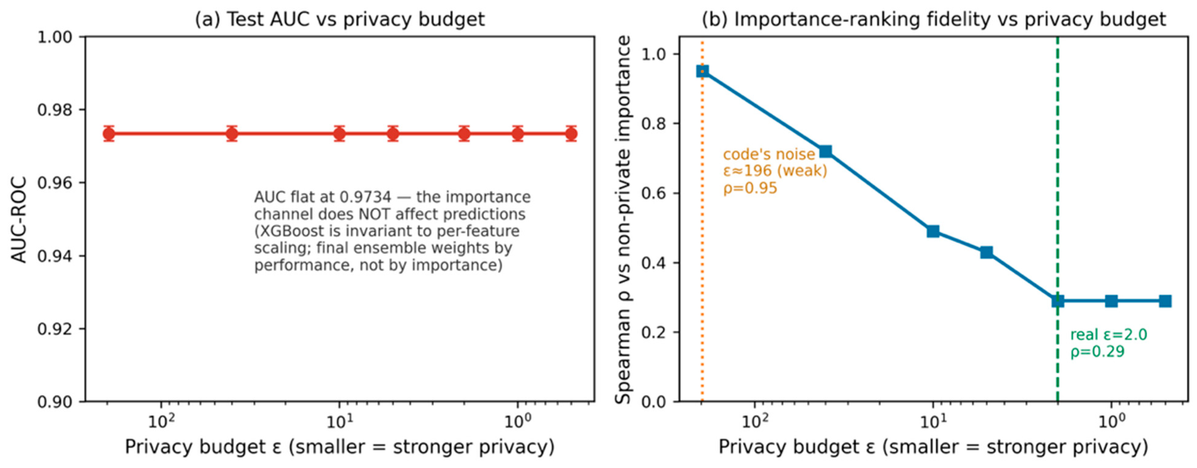
The claim follows because ŷ = f(x) is a deterministic function of inputs that never references φ, so its distribution is unaffected by M(φ) at any ε. The lemma provides a useful diagnostic criterion. In a boosted ensemble, predictions are invariant to per-feature rescaling, and the trees are weighted by performance, not by importance, so feature importance vectors sit off the prediction path; noising them perturbs the interpretation channel and leaves accuracy untouched. A privacy–utility curve that stays flat in ε is therefore evidence that the prediction path was not affected by the privacy mechanism—not evidence that privacy was obtained without utility loss. Section 5.1 demonstrates exactly this; every other experiment places its noise on the prediction path.

Two implications follow from the lemma. First, its contrapositive is the operative design rule: noise placed on a quantity that enters the prediction—a leaf value, a logit, a per-example gradient—makes the predictive distribution depend on ε by construction, so accuracy must move with the budget; a flat privacy–utility curve necessarily means the budget was spent off the prediction path, as Section 5.2 confirms once the noise is moved on-path. Second, off-path privatization can be misleading if interpreted as model-level privacy: noising an interpretation channel while the predictor trains on un-noised data leaves the model with no privacy guarantee, so an adversary with query or parameter access can still mount membership inference or reconstruction attacks—the released importance vector is protected, the model is not. A flat curve therefore indicates that the deployed predictor may remain unprotected.

3.4. Differentially Private Federated Gradient Boosting

The boosting learner takes the additive function-approximation view of gradient boosting [43] with the second-order leaf statistics of XGBoost-style methods [44], but with a data-independent, random split structure, so that tree shape costs no privacy, and the entire budget is spent on leaf statistics. Each round t draws a depth-D tree with random feature–threshold splits; clients route their Poisson-subsampled examples to leaves and accumulate the logistic-loss gradient g = p − y (|g| ≤ 1) and Hessian h = p(1 − p) clipped to [0, 0.25]. Every leaf’s (Σg, Σh) pair has L₂ sensitivity √(1 + 0.25²), is privatized with Gaussian noise of multiplier z, and yields the damped Newton leaf value −η · Σg/(max(Σh, 0) + λ), with the regularization constant fixed at λ = 1.0 in all experiments. The T rounds compose under the accountant described in Section 3.2. Using data-independent splits helps isolate privacy-accounting behavior from tree optimization details.

3.5. Differentially Private Neural and Linear Baselines

The neural baseline is a single-hidden-layer multilayer perceptron (MLP) with rectified linear unit (ReLU) activations under standard DP-SGD [9,45]: per-example gradients clipped to L₂ norm C, Gaussian noise of multiplier z·C added to the clipped sum, Poisson sampling at rate q, T steps composed. The linear baseline strips out the hidden layer—DP-SGD logistic regression—and is included for a specific reason: as the smallest private model, it has fewer parameters to privatize, and so should be the most noise-robust precisely where the budget is tightest. Both baselines are tuned per privacy budget under the same accounting procedure, making them directly comparable references.

3.6. Why Boosting and DP-SGD Respond Oppositely to the Iteration Budget

The two model classes compose noise differently, and this difference, not hypothesis class expressiveness, governs their private behavior.

Proposition 1 (sequential noise accumulation in DP boosting; qualitative).

Because round t fits residuals produced by the noisy rounds < t, privatization noise enters the ensemble state recursively. At a fixed per-round noise multiplier, the variance contributed to the ensemble logit is non-decreasing in the number of rounds T; and holding the total privacy budget fixed forces the per-round multiplier to increase with T under composition. Consequently, the privatized ensemble has a small optimal round count, beyond which added rounds increase prediction noise faster than they reduce bias, and accuracy declines.

We argue Proposition 1 qualitatively here; Appendix A formalizes the monotonicity with a variance bound under independent per-round leaf noise. The mechanism follows from how noise accumulates across boosting rounds. Each privatized leaf value carries additive noise of variance proportional to z², and the additive ensemble sums these contributions across rounds, so for fixed z the logit-noise variance is non-decreasing in T—and since fixed (ε, δ) forces z to grow with T, the effect compounds. DP-SGD is structurally different: its per-step noise is independent across mini-batches and averaged by the optimizer, so under subsampling amplification, more steps reduce the effective noise rather than accumulate it. Both expected behaviors—boosting peaking at a few rounds then decaying, DP-SGD being less sensitive to the step count—are borne out empirically in Section 5.4. This observation motivates the per-budget tuning protocol used in the benchmark: the optimal boosting round count contracts as ε tightens, so a fixed round count systematically under-tunes boosting at exactly the budgets that matter most (quantified in Section 5.3).

4. Experiments

4.1. Datasets and Partitioning

Two real tabular health corpora support the main empirical claims; one synthetic task isolates the mechanism (Table 4). The federation is genuine on 130-US-Hospitals—clients split by medical specialty—and simulated on synthetic and the BRFSS (Behavioral Risk Factor Surveillance System), where records are partitioned across K = 5 clients. Features are standardized from training-set statistics alone; each corpus is split 80/20, and client partitions are frozen across seeds; missing values become a dedicated category, and categories are one-hot encoded. For 130-US-Hospitals, we retain one encounter per patient and drop expired and hospice discharges; BRFSS is binarized to any-diabetes-versus-none and stratified and subsampled; and the synthetic generator draws 8 informative features out of 15. Heterogeneity, participation, and client count ablations appear in Section 5.6.

Table 4. Dataset statistics and client partitioning.

Dataset	n (Train)	d	Prevalence	Partition	Task
Synthetic	4800	15	0.30	Dirichlet(0.5), K = 5	binary
130-US-Hospitals	55,979	101	0.090	by specialty	30-day readmit
BRFSS Diabetes	48,000	21	0.157	simulated, K = 5	diabetes screen

4.2. Models, Search Spaces, and Fair Tuning

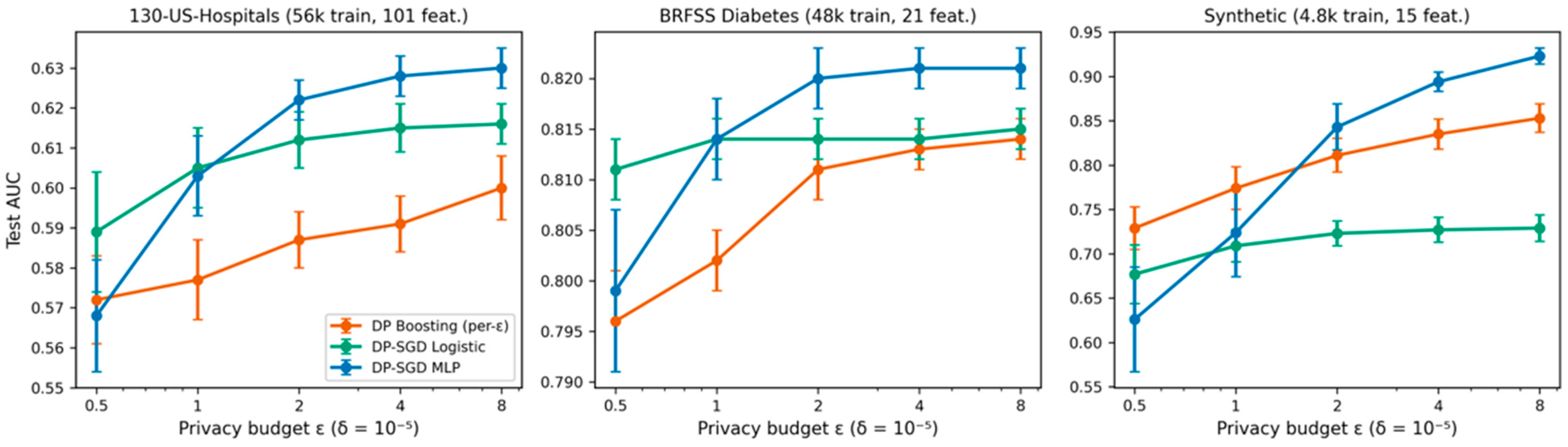
Symmetric tuning is a central safeguard for the comparison. Each method has a comparable hyperparameter budget and—following Proposition 1—is retuned at every privacy budget rather than just once: at each ε, we select the configuration with the best validation AUC, then evaluate on held-out test data over 20 seeds. This is important because the comparison is sensitive to the boosting round count in particular—fixing it across budgets under-tunes boosting at tight ε and can create an apparent neural advantage (Section 5.3)—whereas the network is robust to both its step count and its width. Table 5 lists the search spaces; the selected boosting round count climbs from 25 at ε = 0.5 to 150 at ε = 8, consistent with Proposition 1.

Table 5. Hyperparameter search spaces and selected values.

Model	Hyperparameter (Search Space)	Selected
DP Boosting	rounds T ∈ {25,50,75,100,150}	per-ε (25–150)
DP Boosting	depth ∈ {4,5,6,7}; lr ∈ {0.4,0.5,0.6}; q ∈ {0.03,0.05,0.08}	5; 0.4; 0.05
DP-SGD MLP	hidden ∈ {16,32,64}; steps ∈ {300…1200}	16; 800
DP-SGD MLP	lr ∈ {0.3…3.0}; clip C ∈ {0.5…3.0}; q ∈ {0.02,0.03,0.05}	3.0; 3.0; 0.02
DP-SGD Logistic	lr ∈ {0.5…3.0}; clip C ∈ {1.0…3.0}; q ∈ {0.02,0.05}	2.0; 3.0; 0.02

Symbols: T, boosting rounds; lr, learning rate; q, subsampling rate; C, L₂ clip norm.

Per dataset, the selected boosting round counts across ε ∈ {0.5, 1, 2, 4, 8} are {25, 25, 75, 75, 150} on 130-US-Hospitals, {25, 25, 50, 50, 50} on BRFSS, and {75, 75, 75, 75, 100} on the synthetic task; the noise multiplier for each method is solved per (ε, q, T) using bisection on the PLD accountant. All learners and the accounting pipeline are implemented in Python 3.10 or later using NumPy 1.24 or later, SciPy 1.10 or later, and Matplotlib 3.7 or later, with privacy calibration via Google’s dp-accounting library (version 0.4 or later); the minimum software versions are listed in requirements.txt (File S2 of the Supplementary Materials).

4.3. Evaluation

Because both real corpora are imbalanced (9% and 16% positive), the area under the receiver operating characteristic curve (AUC) is reported alongside the area under the precision–recall curve (AUPRC), with the Brier score for calibration and sensitivity/specificity at the prevalence threshold. Across 20 seeds, we report mean ± standard deviation (SD) with paired t-tests, Wilcoxon signed-rank tests, and Cohen’s d; at 20 seeds, the Wilcoxon test is informative—reaching p < 0.001 wherever a method leads clearly—so we take it as the primary test of significance.

5. Results

5.1. Off-Path Privatization Does Not Protect the Predictor

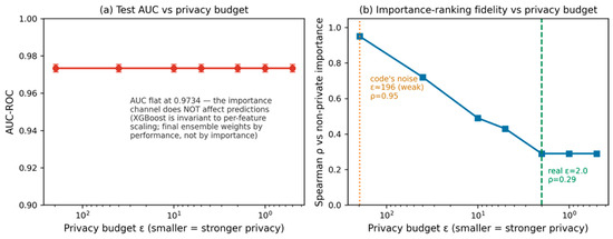
Privatizing the interpretation channel yields a flat privacy–utility curve (Figure 1): test AUC holds constant across two orders of magnitude of the budget, and only the fidelity of the noised importance ranking decays. Consistent with Lemma 1, this indicates that the perturbation does not affect the predictor, and every subsequent experiment therefore places noise on the prediction path.

Figure 1. Off-path privatization leaves test accuracy unchanged while degrading the fidelity of interpretation.

5.2. Under Fair Tuning, No Model Class Dominates

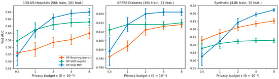
On the prediction path, under matched accounting and per-budget tuning of every method, the three private models achieve similar AUC ranges on both real corpora (Table 6, Figure 2), and the leader changes with dataset and budget. The pattern is consistent across the two real tasks: at the tightest budget the smallest model leads—logistic regression is best at ε = 0.5 on both 130-US-Hospitals (0.589) and BRFSS (0.811), with boosting and the network statistically tied below it (Wilcoxon p = 0.43 and 0.05)—while the network takes a small but significant lead at ε ≥ 1 (up to +0.015 AUC, Wilcoxon p < 0.001, Cohen’s d > 2). Boosting is competitive throughout but is not the single top performer on either real corpus. The nonlinear synthetic task shows a different pattern (Table 6, third block): there, few-round boosting is significantly best at ε ≤ 1 (0.729 vs. the network’s 0.626 at ε = 0.5, Wilcoxon p < 0.001), and the network overtakes it only as the budget loosens, reaching 0.923 vs. 0.853 at ε = 8. The linear model plateaus near 0.72 on synthetic data because the task has genuine feature interactions a linear predictor cannot capture—a contrast with the real corpora, where logistic regression is competitive precisely because these tasks are largely linearly separable. Overall, the leading method varies by dataset and budget: the tight budget winner is whichever frugal model matches the task’s structure—linear for the real tasks, shallow boosting for the nonlinear one—rather than the model class favored in non-private tabular benchmarks.

Table 6. Test AUC under per-budget fair tuning over 20 seeds. Bold indicates the best method at each privacy budget; † indicates a non-significant boosting–MLP difference.

Dataset	ε	DP Boosting	DP-SGD Logistic	DP-SGD MLP
130-US-Hospitals	0.5	0.572 ± 0.011 †	0.589 ± 0.015	0.568 ± 0.014 †
	1	0.577 ± 0.010	0.605 ± 0.010	0.603 ± 0.010
	2	0.587 ± 0.007	0.612 ± 0.007	0.622 ± 0.005
	4	0.591 ± 0.007	0.615 ± 0.006	0.628 ± 0.005
	8	0.600 ± 0.008	0.616 ± 0.005	0.630 ± 0.005
BRFSS Diabetes	0.5	0.796 ± 0.005 †	0.811 ± 0.003	0.799 ± 0.008 †
	1	0.802 ± 0.003	0.814 ± 0.002	0.814 ± 0.004
	2	0.811 ± 0.003	0.814 ± 0.002	0.820 ± 0.003
	4	0.813 ± 0.002	0.814 ± 0.002	0.821 ± 0.002
	8	0.814 ± 0.002	0.815 ± 0.002	0.821 ± 0.002
Synthetic	0.5	0.729 ± 0.024	0.677 ± 0.033	0.626 ± 0.059
	1	0.774 ± 0.024	0.709 ± 0.018	0.724 ± 0.050
	2	0.811 ± 0.019	0.723 ± 0.014	0.843 ± 0.026
	4	0.835 ± 0.017	0.727 ± 0.014	0.894 ± 0.011
	8	0.853 ± 0.016	0.729 ± 0.015	0.923 ± 0.009

Figure 2. Privacy–accuracy curves under per-budget fair tuning over 20 seeds. Error bars indicate ±SD.

The imbalance-aware and calibration metrics indicate the same (Table 7), now with the Wilcoxon signed-rank test, which is informative at 20 seeds. On 130-US-Hospitals, where the positive rate is 9%, and AUC alone is insufficient, the network’s AUPRC matches or exceeds boosting’s at every budget (0.118 vs. 0.113 at ε = 0.5; 0.156 vs. 0.119 at ε = 2). On the BRFSS, the two are tied in AUPRC at ε = 0.5 (0.410 vs. 0.409, p = 0.67), and the network leads thereafter. On synthetic, the crossover is sharp: boosting’s AUPRC is far higher at the tightest budget (0.557 vs. 0.422 at ε = 0.5) and the network’s is higher once the budget loosens (0.875 vs. 0.747 at ε = 8). Brier scores are close on the real corpora and favor boosting at the tightest budgets on the harder synthetic task (0.258 vs. 0.337 at ε = 0.5). The Wilcoxon test confirms the AUC pattern: the network–boosting difference is significant (p < 0.001) and large (Cohen’s d > 2) wherever a method leads clearly, and insignificant exactly where the curves cross—130-Hospitals and BRFSS at ε = 0.5 (p = 0.43 and 0.05), where logistic regression is in fact the leader. At a fixed prevalence threshold, the methods differ in the sensitivity/specificity trade-off—boosting flags more positives (higher recall, lower specificity) while the network is more conservative—but this reflects calibration and operating-point choice rather than discrimination. We report it in full and rely on the threshold-free AUC and AUPRC for the central comparison.

Table 7. AUPRC, Brier score, and boosting–MLP significance tests over 20 seeds. Positive Cohen’s d favors MLP; negative d favors boosting. Bold indicates the higher AUPRC value within each boosting–MLP comparison; † indicates a non-significant Wilcoxon difference (p ≥ 0.05).

Dataset	ε	Boost AUPRC	MLP AUPRC	Boost Brier	MLP Brier	Wilcoxon p	d
130-US-Hosp.	0.5	0.113	0.118	0.082	0.086	0.430 †	−0.2
	1	0.115	0.140	0.081	0.084	<0.001	2.1
	2	0.119	0.156	0.082	0.082	<0.001	4.1
	4	0.121	0.163	0.081	0.081	<0.001	4.2
	8	0.130	0.166	0.081	0.081	<0.001	3.3
BRFSS	0.5	0.410	0.409	0.113	0.118	0.053 †	0.4
	1	0.425	0.447	0.111	0.111	<0.001	3.0
	2	0.436	0.460	0.110	0.109	<0.001	3.0
	4	0.442	0.463	0.109	0.108	<0.001	3.1
	8	0.444	0.465	0.109	0.108	<0.001	3.2
Synthetic	0.5	0.557	0.422	0.258	0.337	<0.001	−1.6
	1	0.619	0.547	0.207	0.280	<0.001	−0.8
	2	0.676	0.742	0.171	0.179	<0.001	1.1
	4	0.716	0.825	0.151	0.136	<0.001	2.7
	8	0.747	0.875	0.142	0.104	<0.001	5.0

5.3. The Comparison Is Fragile to the Boosting Round Count

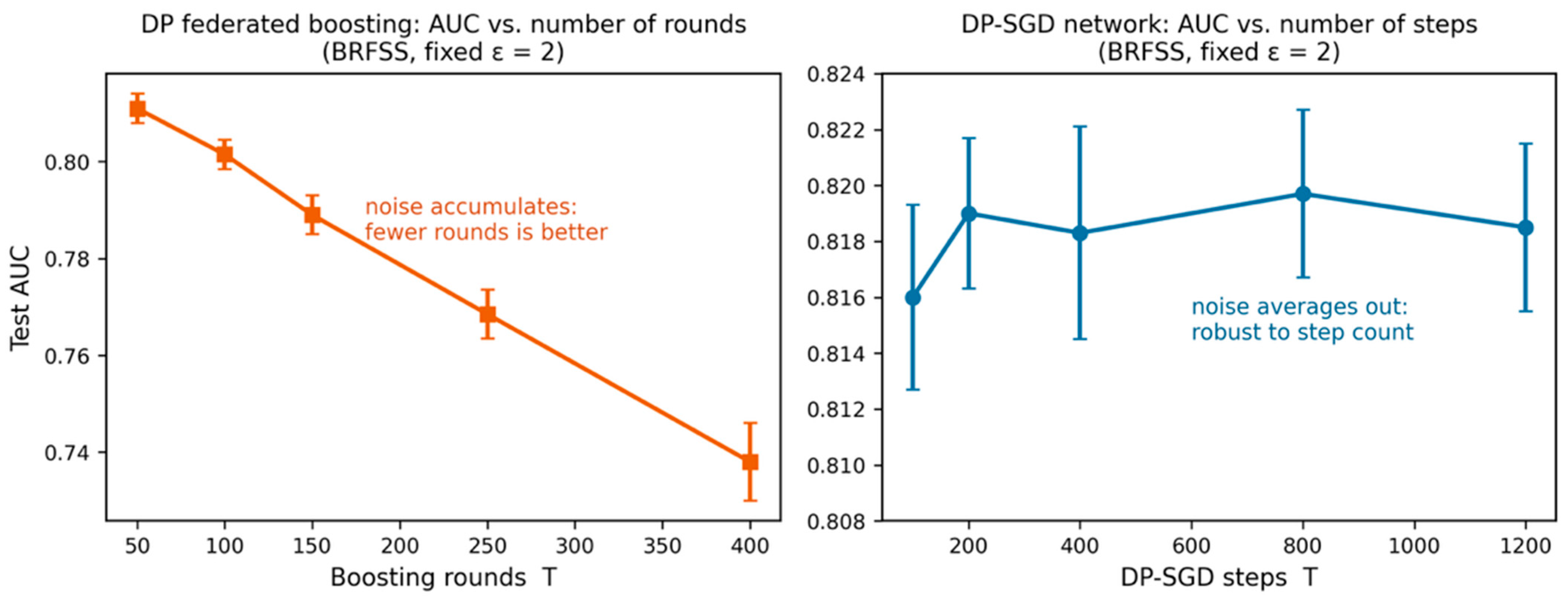
The small, budget-dependent gaps described in Section 5.2 emerge only under symmetric, per-budget tuning, and the fragility is asymmetric: it lies almost entirely on the boosting side. The sensitive hyperparameter is the boosting round count. Holding it fixed across budgets—the natural choice when a method is tuned once and the configuration reused—under-tunes boosting at the budgets where its optimum is small, by exactly the mechanism of Proposition 1. At ε = 2 on BRFSS, a boosting ensemble fixed at T = 150 reaches only 0.789 AUC, against 0.811 when the round count is retuned to its per-budget optimum of T = 50; the same fixed configuration is worse still at ε = 0.5. A practitioner who tunes boosting once at a loose budget and reuses it at tight budgets may therefore observe an apparent network advantage—an artifact of the round count, not of model class.

The network is less sensitive to the corresponding iteration budget choice on these datasets. It is robust to its iteration budget: trained for only 100 steps, it nearly matches the fully tuned 800-step network (0.618 vs. 0.622 on 130-US-Hospitals, 0.816 vs. 0.820 on BRFSS, at ε = 2), consistent with the flat step count curve of Figure 3. Additional capacity also does not improve performance under privacy; widening the hidden layer from 16 to 128 units adds parameters that must each be privatized, and lowers AUC under privacy (0.622 → 0.573 on 130-US-Hospitals, 0.820 → 0.805 on BRFSS at ε = 2). The frugal 16-unit network is already near-optimal under the noise the budget forces. This has a direct benchmarking implication: fair comparisons should retune the boosting round count at every privacy budget, and a study that fixes it may report a neural advantage that is reduced once boosting is retuned per budget (Table 8). This observation helps explain why fixed-round comparisons can yield inconsistent rankings in the prior literature.

Figure 3. Opposite iteration-budget behavior of DP boosting and DP-SGD at ε = 2 on BRFSS.

Table 8. Tuning-fairness ablation at ε = 2. The ablation isolates boosting round-count sensitivity and MLP robustness.

Configuration (ε = 2)	130-Hosp.	BRFSS	Note
Boosting, per-ε rounds (T = 75/50)	0.587	0.811	correct per-budget tuning
Boosting, fixed rounds (T = 150)	0.590	0.789	under-tunes boosting (BRFSS)
Network, fair (T = 800, h = 16)	0.622	0.820	robust baseline
Network, few steps (T = 100)	0.618	0.816	robust to step count
Network, widened (h = 128)	0.573	0.805	extra capacity hurts under DP

5.4. Mechanism

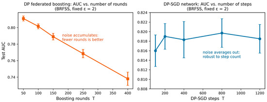
Figure 3 confirms Proposition 1 directly. At a fixed budget (ε = 2 on BRFSS), boosting peaks at very few rounds (T ≈ 25–50) and then declines monotonically—0.811 at 50 rounds down to 0.738 at 400—as per-round noise accumulates through the ensemble. DP-SGD shows the opposite pattern, staying essentially flat from 100 to 1200 steps (≈0.816–0.820) because its independent per-step noise averages out under subsampling amplification. The same structural fact explains both the narrow private gaps described in Section 5.2 and the one-sided tuning fragility described in Section 5.3: boosting performs best at a small, budget-dependent round count that a fixed configuration cannot track, while the network is much less sensitive to its step count.

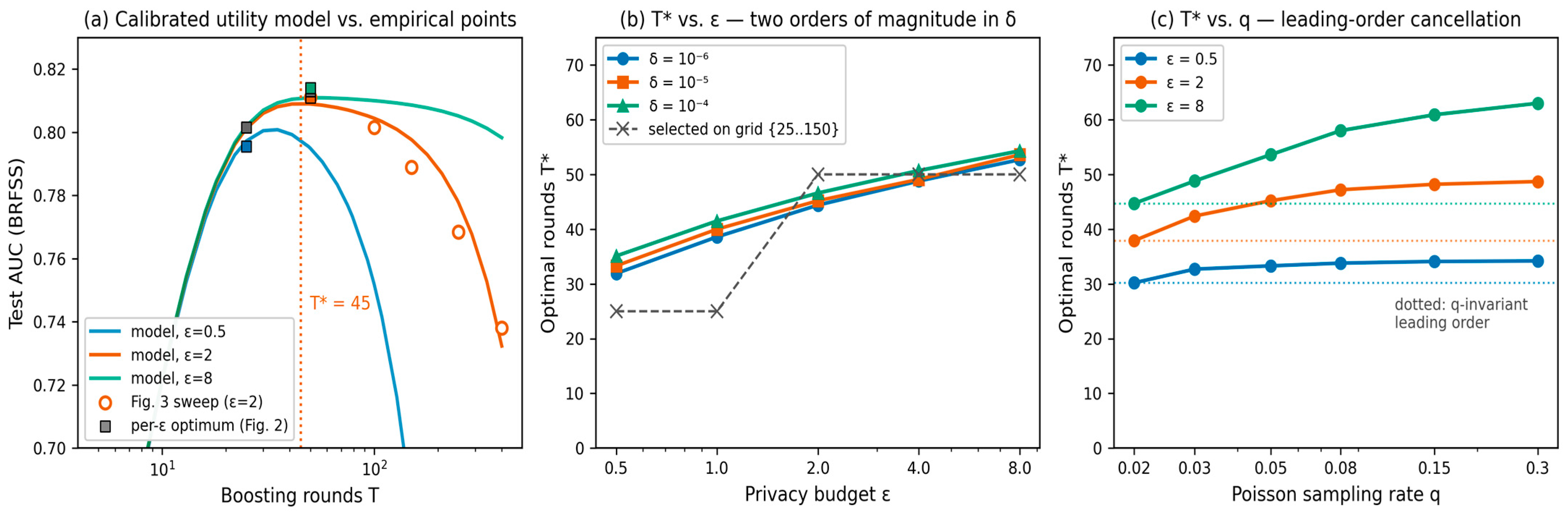
Appendix A.4 makes the boosting round-count optimum explicit: a closed form T* = τ·W₀(A·ε²/(2c·κ²·τ²·log(1/δ))) follows from the variance bound of Appendix A.2. A numerical study under the exact accountant, calibrated on the 20-seed measurements of Figure 2 and Figure 3, quantifies its sensitivity: T* is governed almost entirely by ε (elasticity ≈ 0.17), while two orders of magnitude in δ move it by at most 10% and a 15-fold change in the sampling rate q by only 5–13%. The reason is structural: Poisson subsampling scales the privacy cost and the per-leaf signal by the same factor at leading order, so q nearly cancels. The per-budget round-count grid described in Section 4.2 therefore remains valid across deployment-typical (δ, q), and only ε requires retuning.

5.5. Membership Inference Confirms the Off-Path Risk

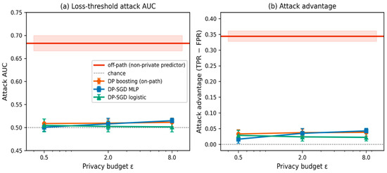
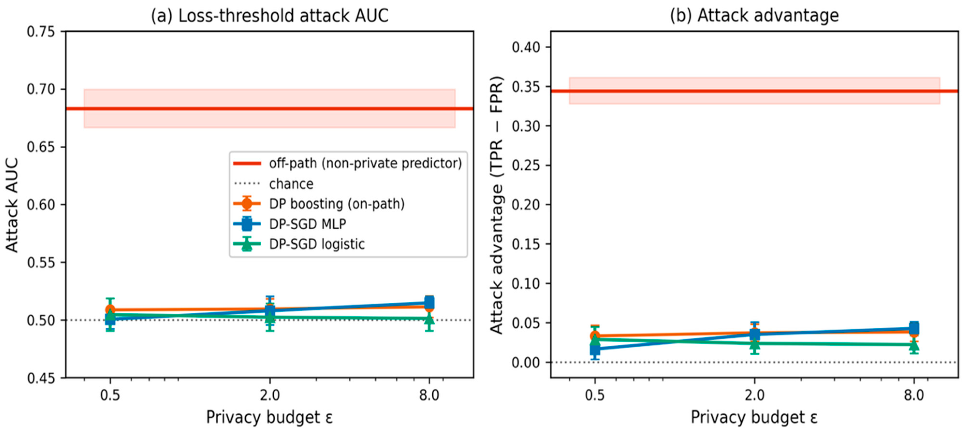
Lemma 1 has a direct attack-side reading: if the budget is spent off the prediction path, the deployed predictor is as exposed as a non-private model at every nominal ε. We test this with the standard loss-threshold membership inference attack: the adversary scores a queried record with its negative prediction loss, and we report the threshold-free attack AUC together with the maximum advantage (TPR − FPR) over thresholds, over 10 seeds on the synthetic mechanism task (members: 1200 training records; non-members: 1200 held-out records; the ablation harness re-instantiates the generator described in Section 4.1, so absolute utility levels are not comparable across tables). The off-path condition is the accuracy-tuned non-private ensemble described in Section 5.1 with the budget spent on the released importance vector; the on-path conditions are the three learners described in Section 4.2.

Table 9 and Figure 4 report the outcome. Against the off-path pipeline, the attack attains an AUC of 0.683 ± 0.017 and an advantage of 0.344 ± 0.017—invariant to the nominal budget by construction, since the predictor never receives noise. Against on-path training, every model class sits at or near chance: boosting at 0.509–0.511 across budgets, logistic regression at ≈0.50, and the MLP rising mildly from 0.501 to 0.515 ± 0.005 at ε = 8; the smallest model leaks least, consistent with its noise robustness profile. The pairing of a flat privacy–utility curve with high attack success is thus the empirical signature of off-path privatization, while record-level on-path DP at these budgets suppresses the attack to near-chance for all three model classes.

Table 9. Loss-threshold membership inference (10 seeds): attack AUC and maximum advantage (ε = 0.5/2/8). Off-path privatization leaves the predictor exposed at every nominal budget.

Model	Attack AUC (ε = 0.5/2/8)	Advantage (ε = 0.5/2/8)
Off-path (any nominal ε)	0.683 ± 0.017 (flat)	0.344 ± 0.017 (flat)
DP boosting (on-path)	0.509/0.510/0.511	0.033/0.037/0.038
DP-SGD logistic	0.505/0.502/0.501	0.029/0.024/0.022
DP-SGD MLP	0.501/0.508/0.515	0.016/0.035/0.043

Figure 4. Loss-threshold membership-inference attack: (a) attack AUC; (b) attack advantage (TPR − FPR). Mean ± SD over 10 seeds. The red shaded band denotes ±SD around the off-path mean.

5.6. Heterogeneity, Participation, and Covariate Shift

Remark 1 (partition invariance under full participation).

Under the aggregation model set out in Section 3.2—full client participation, secure aggregation, and record-level Poisson sampling—each round’s sufficient statistics are sums over a Poisson-q sample of the pooled data: the union of independent per-client Poisson samples is a Poisson sample of D. The statistics are therefore invariant in distribution to the partition {D_k}, so label-skew Dirichlet α, client count K, and client size imbalance cannot affect any of the three learners in this regime. Empirically, α = 0.1 versus α = 10 changes mean AUC by at most 0.011 at ε = 2 (within one standard deviation), confirming the remark.

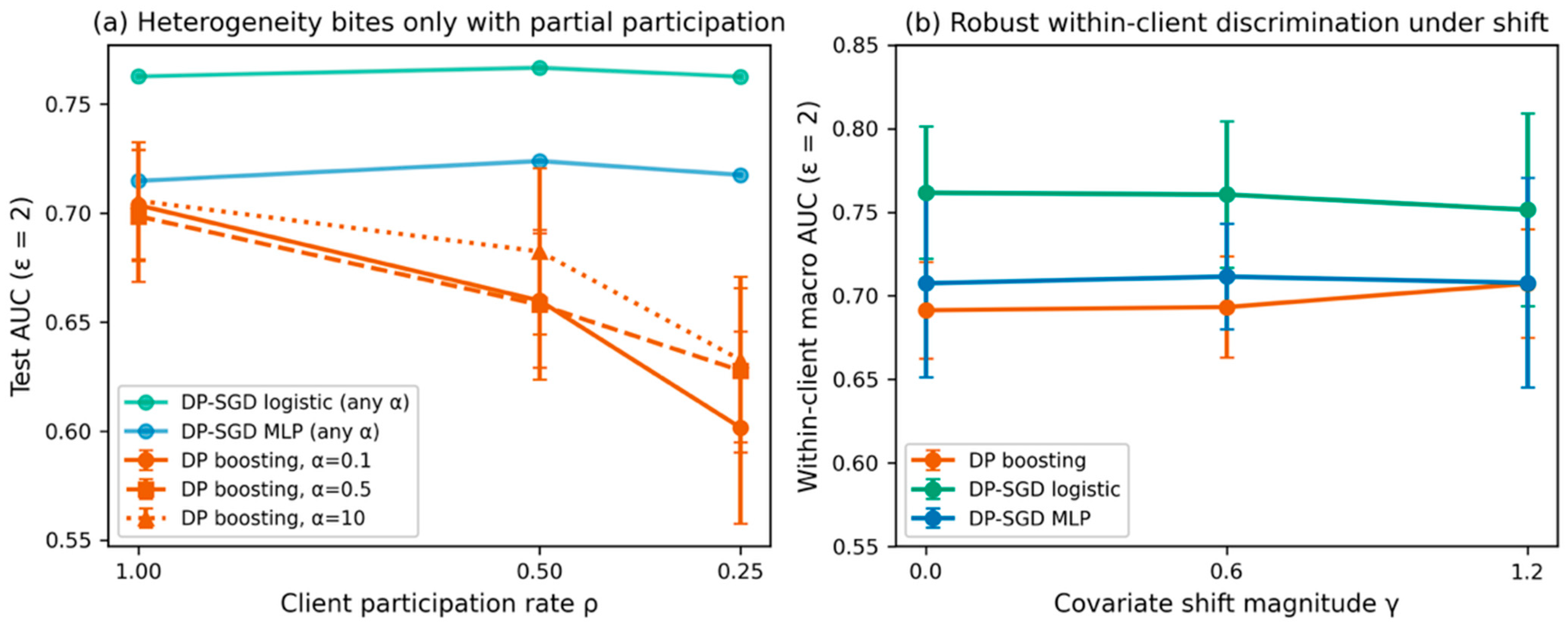
Heterogeneity becomes operative exactly when participation is partial. We therefore sweep a client participation rate ρ ∈ {1.0, 0.5, 0.25}—each round, clients respond independently with probability ρ—crossed with α ∈ {0.1, 0.5, 10}, holding the privacy budget fixed by recalibrating the noise multiplier at the effective rate q_eff = ρq (client Poisson composed with record Poisson is record-level Poisson at ρq). Table 10 shows the outcome at ε = 2 over 10 seeds: boosting loses 7–10 AUC points at ρ = 0.25 and the loss grows with skew (0.602 ± 0.044 at α = 0.1 versus 0.633 ± 0.038 at α = 10), whereas DP-SGD logistic and the MLP move by at most 0.01 across the entire grid. The mechanism is the one formalized in Proposition 1: each boosting round fits residuals produced by earlier rounds, so rounds computed on skewed client subsets inject bias that the sequential structure cannot average away, while DP-SGD’s independent per-step noise and gradient averaging absorb the same perturbation. Client count K ∈ {5, 10, 20} and Zipf-1.5 size imbalance show no systematic effect at ρ = 0.5.

Table 10. Participation × heterogeneity at ε = 2 (test AUC over 10 seeds). Partial participation harms boosting, and more so under label skew; DP-SGD is unaffected.

Model	ρ = 1.0	ρ = 0.5	ρ = 0.25
DP boosting, α = 0.1	0.704 ± 0.026	0.660 ± 0.031	0.602 ± 0.044
DP boosting, α = 0.5	0.698 ± 0.030	0.658 ± 0.034	0.628 ± 0.038
DP boosting, α = 10	0.706 ± 0.027	0.682 ± 0.038	0.633 ± 0.038
DP-SGD logistic (any α)	0.763 ± 0.059	0.767 ± 0.058	0.763 ± 0.058
DP-SGD MLP (any α)	0.715 ± 0.050	0.724 ± 0.054	0.717 ± 0.053

Finally, we probe feature distribution shift: each client’s covariates are mean-shifted along a client-specific direction of magnitude γ ∈ {0, 0.6, 1.2} under a shared labeling concept, and models are evaluated on held-out data from the same mixture of client distributions. Within-client discrimination—macro-averaged AUC across clients—is flat for all three learners (boosting 0.691 → 0.693 → 0.707 at ε = 2; differences within one SD), so no model class is differentially fragile to covariate shift in this design. We add a methodological caution: pooled AUC inflates under shift (0.692 → 0.836 for boosting) purely through between-client separability and should not be read as robustness; the within-client metric is the informative one. Figure 5 summarizes both findings; scripts for all sweeps are in the public artifact.

Figure 5. Heterogeneity ablations at ε = 2: (a) test AUC versus client-participation rate ρ at three label-skew levels; (b) within-client macro AUC versus covariate-shift magnitude γ. Mean ± SD over 10 seeds.

6. Discussion

RQ1 and RQ2 are answered jointly: the non-private tabular advantage of trees does not translate into a differentially private federated advantage, and the private regime does not favor neural networks either. Under matched accounting and fair tuning, the three model classes are close in accuracy, and the apparent neural advantage reported under a fixed boosting round count is a tuning artifact that is removed once the round count is retuned per budget. RQ3 is answered by Proposition 1 and Figure 3: the classes differ in how they compose noise, not in expressiveness, and this difference both narrows the private gap and makes the comparison tuning-sensitive.

6.1. Implications for Private Healthcare AI and for Benchmarking

For practitioners, the practical implication is that several model classes remain viable under privacy: the choice among a boosted ensemble, a small network, and a logistic model is less decisive than non-private tabular results might suggest, and a parameter-frugal model—even DP logistic regression—is competitive throughout, with an advantage at the tightest budgets. The secure-aggregation and integrity components of a federated protocol are important but model-agnostic; they transfer unchanged across these models and should be interpreted as infrastructure-level benefits rather than accuracy effects. For the field’s methodology, three safeguards follow directly: place DP noise on the prediction path and treat budget-invariant accuracy as a warning sign; account all methods under one procedure; and tune neural, linear, and tree baselines symmetrically and per budget, retuning the boosting round count at every budget in particular. Because the accuracy differences are small, communication cost becomes a more informative basis for model choice (Section 6.2).

6.2. Communication Cost Favors Boosting

Accuracy is not the only axis of comparison, and with respect to communication volume, boosting has a clear communication advantage. In each synchronization round, a boosting client uploads only the privatized leaf statistic vector—two values per leaf, 2·2^D = 64 floats for the depth-5 trees used here—whereas a DP-SGD client uploads the full clipped parameter gradient at every step: P·h + 2h + 1 values for the network and P + 1 for logistic regression. Multiplied by the iteration counts (25–150 boosting rounds against 800 DP-SGD steps), the totals differ by one to three orders of magnitude (Table 11). On 130-US-Hospitals, the network transmits 1.3 million floats per client against boosting’s 1600–9600—a 137×–824× gap—and even logistic regression, with substantially fewer parameters than the network, sends 9×–51× more than boosting. Boosting also needs far fewer synchronization rounds, which, in a federated deployment, translates directly into fewer round-trips and lower exposure to slow-client delays. Secure aggregation changes how these payloads are combined at the server, not the size each client sends, so the reported ratios are unaffected. This distinction is practically important when accuracy differences are small. Where bandwidth or round-trip latency binds—cross-silo healthcare federation over wide-area links, or cross-device settings—boosting’s lower communication cost is a substantial practical advantage, independent of its statistically negligible accuracy difference.

Table 11. Per-client communication volume under fair tuning. Values are the total number of uploaded floats; server broadcast and cryptographic overhead are excluded.

Dataset	Boosting (ε = 0.5 → 8)	DP-SGD MLP	DP-SGD Logistic	MLP/Boost
130-US-Hospitals	1600–9600	1,319,200	81,600	137×–824×
BRFSS Diabetes	1600–3200	295,200	17,600	92×–184×
Synthetic	4800–6400	218,400	12,800	34×–46×

The compute side of deployment cost is modest for all learners. In our reference implementation (single CPU core), a boosting client’s per-round work—routing its Poisson sample through the round’s tree and accumulating per-leaf sums—costs ≈ 0.10 ms per 1000 client records and is linear in the shard size; full training on the synthetic task takes 0.24 s (boosting, T = 75), 0.17 s (logistic, 800 steps), and 0.52 s (MLP, 800 steps), with incremental peak memory below 1 MB beyond the data itself. Privacy accounting adds a one-off ≈ 0.4 s bisection per (ε, q, T) configuration—a privacy-loss distribution evaluation cross-checked against Rényi—which is cached and amortized across seeds. Scaling these linear costs to the largest corpus keeps client-side training in the seconds-to-minutes range on commodity silo hardware: compute is not the binding resource; communication and synchronization are.

Communication volume translates directly into synchronization time. With synchronous rounds, total synchronization cost is R·(RTT + payload/bandwidth) over R round-trips; Table 12 evaluates three link profiles with the 130-US-Hospitals payloads. Because every learner’s payload is small relative to bandwidth (256 B per round for boosting; ≈6.6 kB per step for the network), the round-trip count dominates: over a cross-silo WAN (50 ms RTT, 100 Mbit/s), boosting synchronizes in 1.3–7.5 s against ≈40 s for the 800-step DP-SGD baselines—a 5–32× gap that widens on constrained links (3.8–22.5 s versus ≈120–124 s). Each synchronization barrier is also an exposure to stragglers, so the low-round-count learner gains twice.

Table 12. Analytic synchronization time R·(RTT + payload/bandwidth); 130-US-Hospitals payloads.

Link Profile	DP Boosting (25–150 Rounds)	DP-SGD Logistic (800 Steps)	DP-SGD MLP (800 Steps)
LAN (1 ms, 1 Gbit/s)	0.03–0.15 s	0.8 s	0.8 s
Cross-silo WAN (50 ms, 100 Mbit/s)	1.3–7.5 s	40.0 s	40.4 s
Constrained (150 ms, 10 Mbit/s)	3.8–22.5 s	120.3 s	124.2 s

Secure aggregation adds a quantifiable, model-independent overhead that Table 11 excludes by design. In Bonawitz et al.’s protocol [42], each client per round performs pairwise key agreement and uploads masking material of O(K) small constants (≈32–64-byte keys and shares per peer)—a few kilobytes at the K = 5–20 cross-silo scales considered here—while the masked-sum payload itself is unchanged in size and the server performs O(K²) reconstruction work. Because the identical wrapper applies to every learner, the ratios of Table 11 and the estimates of Table 12 are unaffected, and boosting’s advantage, driven by round count and payload size, is preserved under the cryptographic deployment assumed in Section 3.2.

6.3. Relation to Prior Differentially Private Boosting Results

The closest prior work, Maddock et al. [24], decomposes federated DP-GBDT into its algorithmic components and compares boosting variants against one another; they report that their per-round and histogram-based methods peak at roughly 25–50 trees while a third variant needs hundreds—an observation that directly corroborates Proposition 1, since under a fixed budget, accumulated per-round noise caps the useful round count. Our independent reimplementation reproduces the same qualitative optimum: the per-budget boosting round count selected here ranges from 25 at the tightest budget to 150 at the loosest (Figure 3). The present study addresses a different comparison: boosting versus DP-SGD baselines under a shared accountant. Maddock et al. compare boosting designs to each other under their own accountant; we instead hold a single PLD accountant fixed across model classes and add the DP-SGD and DP-logistic baselines that their study does not consider. The main result, that no model class dominates and that the boosting round count is the sensitive hyperparameter, is difficult to observe in a boosting-only comparison. The agreement on the round-count mechanism, reached independently and under different accounting, suggests that the effect is structural and consistent across independently developed boosting constructions.

6.4. When Boosting Remains the Right Choice, and Interpreting Absolute Performance

The narrow private band partly reflects the modest headroom of the two real tabular health tasks. Stripped of privacy, the three model classes reach an AUC near 0.64 on 130-US-Hospitals and near 0.82 on the BRFSS—within about 0.02 of one another—so readmission and screening leave little headroom for any model to exploit, and DP at ε = 8 forfeits only 0.01–0.03 AUC. The synthetic task is a useful contrast: there, the non-private tree (0.946) slightly exceeds the non-private network (0.934), confirming the tabular tree advantage when nonlinear structure is present—yet privacy still inverts the ranking at loose budgets. Any non-private gap is substantially reduced once prediction-path privacy noise is introduced.

This conclusion is specific to the studied record-level DP, horizontal-federation setting. Boosting remains attractive in non-private or weak-privacy federations, cryptographic privacy settings, interpretability-first deployments, vertical federation, and small-data regimes. Within this setting, boosting offers no accuracy advantage, although it has substantially lower communication cost.

The absolute AUC on 130-US-Hospitals is modest (≈0.6)—expected for 30-day readmission at a 9% positive rate with non-private ceilings near 0.63—but the focus of this benchmark is the relative behavior of private learners across privacy budgets, and the imbalance-aware AUPRC indicates the same. The BRFSS, far easier in absolute terms (≈0.82), reproduces the qualitative picture exactly, so the qualitative pattern is not limited to the harder readmission task.

7. Limitations

Several limitations affect the scope of this benchmark. First, we instantiate one reasonable private mechanism per model class—four classes, with the parallel-composition random forest of Appendix B—rather than evaluating all private boosting variants or neural architectures. Tabular-specific private networks, such as attention-based models, are excluded deliberately, since our width ablation (Table 8) and prior evidence [37] indicate that added neural capacity suffers under differential privacy at these sample sizes. Second, federation is genuine on 130-US-Hospitals and simulated elsewhere; Section 5.6 covers heterogeneity, participation, client count, imbalance, and covariate shift, but real multi-institution deployment and very large client counts remain untested. Third, this study is focused by design on central, record-level, horizontal DP with trusted aggregation (Section 3.2): client-level DP is a strictly different granularity with its own composition behavior [16], local DP changes the trust model and the location of the noise, and vertical partitioning changes the mechanism design entirely [6,23]—mixing these regimes within one benchmark would break precisely the matched-accounting comparability this study contributes, so each is future work rather than an omission. Fourth, we report membership inference audits (Section 5.5) and deployment costs (Section 6.2), but poisoning robustness, Byzantine clients, subgroup fairness, and reconstruction attacks remain open. Within this scope, the results support the conclusion that the non-private tree advantage does not translate into a differentially private federated accuracy advantage under matched accounting, symmetric tuning, and prediction-path privacy.

8. Future Work

Future work should extend the benchmark to naturally partitioned multi-institution datasets such as FLamby Fed-Heart-Disease, sweep client heterogeneity and client counts, and add empirical membership inference and reconstruction audits for both off-path and prediction-path mechanisms.

9. Conclusions

Under matched accounting and fair, per-budget tuning, differentially private federated gradient boosting, a DP-SGD network, and DP-SGD logistic regression are close on the accuracy axis for tabular healthcare data, with no model class dominating: on the real corpora, the most frugal model—logistic regression—is best at the tightest budget, and the network holds a small edge at looser ones, while boosting leads only on the nonlinear synthetic task at the tightest budgets. The non-private tabular advantage of trees does not translate into a private accuracy advantage, but neither does a neural one. We identify two sources of misleading conclusions: off-path privatization, which leaves the prediction path unaffected, and fixed-round boosting comparisons, which can create an apparent neural advantage. We further explain the latter through the distinct noise-composition behavior of boosting and DP-SGD, which we formalize and confirm. A practical implication is that future private tabular federated studies should report whether their DP noise is on the prediction path, account for all methods under a single procedure, and tune neural, linear, and tree baselines symmetrically and per budget. The matched-accounting protocol we define provides a reproducible basis for such comparisons.

Appendix A.1. A Concentration Bound on the Injected Logit Noise

Because F_T(x) − E[F_T(x)] is a sum of independent Gaussians, it is itself Gaussian with variance V_T: = Var[F_T(x)] = Σ_{t ≤ T} σ_t², and therefore sub-Gaussian: for any τ > 0,

P(|F_T(x) − E F_T(x)| > τ) ≤ 2 exp(−τ²/(2 V_T)).

A test point is misclassified by noise when the perturbation crosses the margin between its clean logit and the decision threshold; the bound shows that the probability of such a crossing increases monotonically with V_T. Controlling accuracy under privacy thus reduces to the problem of controlling V_T, which, as the next step shows, grows superlinearly in the round count.

Appendix A.2. Budget-Constrained Noise Grows Quadratically in the Round Count

Fix the target (ε, δ) and the Poisson rate q. Under Rényi composition, the Rényi divergence of T subsampled-Gaussian releases grows linearly in T, so holding ε fixed forces the per-round multiplier to scale as z(T) = Θ(√(T)) up to logarithmic factors (more releases demand proportionally more noise per release). Since each σ_t² ∝ z(T)² and there are T such terms,

V_T = Σ_{t ≤ T} σ_t² ∝ T · z(T)² = Θ(T²/ε²).

The injected logit-noise variance is therefore quadratic in the number of rounds at a fixed budget, and inversely quadratic in ε. This is the quantitative form of Proposition 1: added rounds reduce bias but inflate noise variance as T², so the test loss ≈ bias(T) + c·V_T, with bias(T) decreasing and convex, is minimized at a finite, typically small T*.

Corollary A1 (optimal round count contracts with the budget).

Model the privatized test loss as L(T) = B(T) + c·a(ε)·T² with B decreasing and convex and a(ε) = Θ(1/ε²) the per-round noise coefficient. The minimizer T*(ε) satisfies −B′(T*) = 2c·a(ε)·T*, whose right-hand side increases as ε shrinks; hence, T*(ε) is non-decreasing in ε. A fixed round count therefore over-boosts at tight budgets and under-boosts at loose ones.

The corollary matches the selected per-budget optima (T* rising from 25 at ε = 0.5 to 150 at ε = 8) and explains the asymmetric tuning fragility described in Section 5.3: only the boosting round count must move with the budget.

Appendix A.3. Contrast with DP-SGD

DP-SGD does not exhibit the same form of accumulation as the T² growth. For a convex objective, the DP-SGD excess empirical risk is O(√(d · log(1/δ))/(nε)) and is attained by averaging the iterates [25]; the privacy noise enters through a 1/n-scaled average over steps and does not accumulate with the step count. Additional steps reduce the optimization error toward this floor without raising it, which is precisely the flat step count response observed in Figure 3 and the reason the network is robust to its iteration budget, whereas boosting is more sensitive to it. The two model classes thus differ not in expressiveness but in how privacy noise composes—averaged for DP-SGD, accumulated for boosting—and this distinction helps explain the narrow private gap, the small optimal boosting round count, and the one-sided tuning fragility.

Appendix A.4. The Optimal Round Count Under Varying δ and Sampling Rate q

Appendix A.2 established that, at a fixed budget, the injected logit-noise variance grows as V_T ∝ T²/ε². Here, we make the resulting optimum explicit and quantify its sensitivity to the failure probability δ and the Poisson sampling rate q—first in closed form under a leading-order accounting approximation, then numerically under the exact accountant described in Section 3.2. Following Corollary A1, write the privatized test loss as

L(T; ε, δ, q) = A·exp(−T/τ) + c·T·(z(T; ε, δ, q)/q)²

(A1)

where the first term is the decreasing, convex bias of the ensemble and the second is the accumulated leaf noise variance described in Appendix A.1: each round contributes noise of standard deviation proportional to z on leaf statistics whose expected magnitude scales with the Poisson-subsampled leaf count, itself proportional to q, so the per-round noise-to-signal ratio is proportional to z/q and T independent rounds sum. The multiplier z(T; ε, δ, q) is the smallest per-round noise level at which T-fold composition of the Poisson-subsampled Gaussian meets (ε, δ)—the bisection described in Section 4.2. For small q and moderate Rényi orders, one release costs Θ(q²α/z²), so composition at budget (ε, δ) forces

z(T; ε, δ, q) = Θ(q·√(T·log(1/δ))/ε)

(A2)

Substituting (A2) into (A1), the sampling rate cancels—Poisson subsampling scales the privacy cost and the per-leaf signal by the same factor q—and the noise term becomes Θ(c·T²·log(1/δ)/ε²), recovering the T²/ε² law of A.2 with its δ-dependence explicit. Setting ∂L/∂T = 0 and writing x = T/τ gives x·eˣ = Aε²/(2cκ²τ²·log(1/δ)), i.e., a closed-form optimum on the principal Lambert-W branch:

T*(ε, δ) = τ·W₀(A·ε²/(2·c·κ²·τ²·log(1/δ)))

(A3)

Three predictions follow: T* increases with ε only through W₀, so the growth is slow, consistent with the shallow climb of the selected round counts in Table 5; δ enters only inside the logarithm inside W₀, a doubly damped dependence; and q is absent at leading order, so any observed q-dependence must come from the regime where the small-q amplification approximation bends. We verify all three numerically. We calibrate (A1) on this study’s own 20-seed BRFSS measurements—the five-point round sweep presented in Figure 3 (ε = 2) and the five per-budget optima underlying Figure 2—with z computed using bisection at every grid point (Rényi accounting over integer orders 2–512). The four-parameter fit attains RMSE 0.0048 AUC (R² = 0.957), and its continuous optimum reproduces the tuning outcome described in Section 4.2: T* rises from ≈33 at ε = 0.5 to ≈54 at ε = 8, snapping onto the selected values {25, 25, 50, 50, 50} on the search grid {25, 50, 75, 100, 150}. Table A1 and Figure A1 report T* resolved over δ ∈ {10⁻⁶, 10⁻⁵, 10⁻⁴} at q = 0.05 and over q ∈ {0.02, …, 0.30} at δ = 10⁻⁵.

Table A1. Optimal round count T* under the exact accountant (δ sweep at q = 0.05; q sweep at δ = 10⁻⁵).

ε	δ = 10−6	δ = 10−5	δ = 10−4	q = 0.02	q = 0.05	q = 0.30
0.5	31.9	33.3	35.1	30.2	33.3	34.2
1	38.6	40.0	41.5	34.8	40.0	41.7
2	44.4	45.2	46.6	37.9	45.2	48.7
4	48.8	49.1	50.7	42.0	49.1	56.4
8	52.7	53.6	54.3	44.7	53.6	63.0

Table A1. Optimal round count T* under the exact accountant (δ sweep at q = 0.05; q sweep at δ = 10⁻⁵).

ε	δ = 10−6	δ = 10−5	δ = 10−4	q = 0.02	q = 0.05	q = 0.30
0.5	31.9	33.3	35.1	30.2	33.3	34.2
1	38.6	40.0	41.5	34.8	40.0	41.7
2	44.4	45.2	46.6	37.9	45.2	48.7
4	48.8	49.1	50.7	42.0	49.1	56.4
8	52.7	53.6	54.3	44.7	53.6	63.0

The elasticities implied in Table A1 quantify the sensitivity of Proposition 1: ∂ln T*/∂ln ε ≈ 0.17 across the tested range; a two-order-of-magnitude change in δ moves T* by at most 10% (1–3 rounds); and ∂ln T*/∂ln q lies between ≈0.05 at ε = 0.5 and ≈0.13 at ε = 8 over a 15-fold range—the deviation from exact leading-order cancelation grows with the budget because subsampling amplification is nonlinear at moderate q. The optimum is therefore governed almost entirely by ε; δ and q are second-order, so the per-budget tuning protocol described in Section 4.2 needs to track only ε, and the closed form (A3)—within ≈ 10% of the exact-accountant optimum—can initialize the grid search. Calibrating z with the PLD accountant instead of Rényi yields uniformly smaller multipliers, z_PLD/z_RDP ∈ [0.909, 0.941] over T ∈ {25, …, 400} (mean 0.927); the near-constant ratio is absorbed by the fitted constant c and moves the optimum by about one round (T* = 45.2 → 46.3), so the conclusions are insensitive to the choice of accountant.

Figure A1. The optimal boosting round count T* under the exact accountant: (a) the calibrated utility model against the 20-seed BRFSS measurements; (b) T* versus ε for δ ∈ {10⁻⁶, 10⁻⁵, 10⁻⁴}; (c) T* versus the sampling rate q at δ = 10⁻⁵. In (b), the grey dashed line denotes the per-budget grid selection of Section 4.2; dotted lines mark the fitted optimum in (a) and the q-invariant leading-order level in (c).

Figure A1. The optimal boosting round count T* under the exact accountant: (a) the calibrated utility model against the 20-seed BRFSS measurements; (b) T* versus ε for δ ∈ {10⁻⁶, 10⁻⁵, 10⁻⁴}; (c) T* versus the sampling rate q at δ = 10⁻⁵. In (b), the grey dashed line denotes the per-budget grid selection of Section 4.2; dotted lines mark the fitted optimum in (a) and the q-invariant leading-order level in (c).

References

- Grinsztajn, L.; Oyallon, E.; Varoquaux, G. Why Do Tree-Based Models Still Outperform Deep Learning on Typical Tabular Data? Adv. Neural Inf. Process. Syst. 2022, 35, 507–520. [Google Scholar] [CrossRef] [Scilit]
- Shwartz-Ziv, R.; Armon, A. Tabular Data: Deep Learning Is Not All You Need. Inf. Fusion 2022, 81, 84–90. [Google Scholar] [CrossRef] [Scilit]
- McMahan, H.B.; Moore, E.; Ramage, D.; Hampson, S.; Agüera y Arcas, B. Communication-Efficient Learning of Deep Networks from Decentralized Data. In Proceedings of the International Conference on Artificial Intelligence and Statistics (AISTATS); PMLR: London, UK, 2017; pp. 1273–1282. [Google Scholar]
- Kairouz, P.; McMahan, H.B. Advances and Open Problems in Federated Learning. Found. Trends Mach. Learn. 2021, 14, 1–210. [Google Scholar] [CrossRef] [Scilit]
- Li, Q.; Wu, Z.; Wen, Z.; He, B. Privacy-Preserving Gradient Boosting Decision Trees. Proc. AAAI Conf. Artif. Intell. 2020, 34, 784–791. [Google Scholar] [CrossRef] [Scilit]
- Cheng, K.; Fan, T.; Jin, Y.; Liu, Y.; Chen, T.; Papadopoulos, D.; Yang, Q. SecureBoost: A Lossless Federated Learning Framework. IEEE Intell. Syst. 2021, 36, 87–98. [Google Scholar] [CrossRef] [Scilit]
- Dwork, C.; Roth, A. The Algorithmic Foundations of Differential Privacy. Found. Trends Theor. Comput. Sci. 2014, 9, 211–407. [Google Scholar] [CrossRef] [Scilit]
- Dwork, C.; McSherry, F.; Nissim, K.; Smith, A. Calibrating Noise to Sensitivity in Private Data Analysis. In Proceedings of the Theory of Cryptography Conference (TCC); Springer: Berlin/Heidelberg, Germany, 2006; pp. 265–284. [Google Scholar]
- Abadi, M.; Chu, A.; Goodfellow, I.; McMahan, H.B.; Mironov, I.; Talwar, K.; Zhang, L. Deep Learning with Differential Privacy. In Proceedings of the ACM SIGSAC Conference on Computer and Communications Security (CCS); ACM: New York, NY, USA, 2016; pp. 308–318. [Google Scholar]
- Mironov, I. Rényi Differential Privacy. In Proceedings of the IEEE Computer Security Foundations Symposium (CSF); IEEE: New York, NY, USA, 2017; pp. 263–275. [Google Scholar]
- Wang, Y.-X.; Balle, B.; Kasiviswanathan, S.P. Subsampled Rényi Differential Privacy and Analytical Moments Accountant. In Proceedings of the International Conference on Artificial Intelligence and Statistics (AISTATS); PMLR: London, UK, 2019; pp. 1226–1235. [Google Scholar]
- Zhu, Y.; Wang, Y.-X. Poisson Subsampled Rényi Differential Privacy. In Proceedings of the 36th International Conference on Machine Learning (ICML), Long Beach, CA, USA, 9–15 June 2019; PMLR: London, UK, 2019; Volume 97, pp. 7634–7642. [Google Scholar]
- Dong, J.; Roth, A.; Su, W.J. Gaussian Differential Privacy. J. R. Stat. Soc. B 2022, 84, 3–37. [Google Scholar] [CrossRef] [Scilit]
- Koskela, A.; Jälkö, J.; Honkela, A. Computing Tight Differential Privacy Guarantees Using FFT. In Proceedings of the International Conference on Artificial Intelligence and Statistics (AISTATS); PMLR: London, UK, 2020; pp. 2560–2569. [Google Scholar]
- Gopi, S.; Lee, Y.T.; Wutschitz, L. Numerical Composition of Differential Privacy. Adv. Neural Inf. Process. Syst. 2021, 34, 11631–11642. [Google Scholar]
- McMahan, H.B.; Ramage, D.; Talwar, K.; Zhang, L. Learning Differentially Private Recurrent Language Models. In Proceedings of the 6th International Conference on Learning Representations (ICLR), Vancouver, BC, Canada, 30 April–3 May 2018. [Google Scholar]
- Truex, S.; Baracaldo, N.; Anwar, A.; Steinke, T.; Ludwig, H.; Zhang, R.; Zhou, Y. A Hybrid Approach to Privacy-Preserving Federated Learning. In Proceedings of the ACM Workshop on Artificial Intelligence and Security (AISec); ACM: New York, NY, USA, 2019; pp. 1–11. [Google Scholar]
- Friedman, A.; Schuster, A. Data Mining with Differential Privacy. In Proceedings of the ACM SIGKDD International Conference on Knowledge Discovery and Data Mining; ACM: New York, NY, USA, 2010; pp. 493–502. [Google Scholar]
- Jagannathan, G.; Pillaipakkamnatt, K.; Wright, R.N. A Practical Differentially Private Random Decision Tree Classifier. In Proceedings of the IEEE International Conference on Data Mining Workshops (ICDMW); IEEE: New York, NY, USA, 2009; pp. 114–121. [Google Scholar]
- Fletcher, S.; Islam, M.Z. Differentially Private Random Decision Forests Using Smooth Sensitivity. Expert Syst. Appl. 2017, 78, 16–31. [Google Scholar] [CrossRef] [Scilit]
- Nori, H.; Caruana, R.; Bu, Z.; Shen, J.H.; Kulkarni, J. Accuracy, Interpretability, and Differential Privacy via Explainable Boosting. In Proceedings of the International Conference on Machine Learning (ICML); PMLR: London, UK, 2021; pp. 8227–8237. [Google Scholar]
- Li, Q.; Wen, Z.; He, B. Practical Federated Gradient Boosting Decision Trees. Proc. AAAI Conf. Artif. Intell. 2020, 34, 4642–4649. [Google Scholar] [CrossRef] [Scilit]
- Tian, Z.; Zhang, R.; Hou, X.; Lyu, L.; Zhang, T.; Liu, J.; Ren, K. FederBoost: Private Federated Learning for GBDT. IEEE Trans. Dependable Secur. Comput. 2024, 21, 1274–1285. [Google Scholar] [CrossRef] [Scilit]
- Maddock, S.; Cormode, G.; Wang, T.; Maple, C.; Jha, S. Federated Boosted Decision Trees with Differential Privacy. In Proceedings of the ACM SIGSAC Conference on Computer and Communications Security (CCS); ACM: New York, NY, USA, 2022; pp. 2249–2263. [Google Scholar]
- Bassily, R.; Smith, A.; Thakurta, A. Private Empirical Risk Minimization: Efficient Algorithms and Tight Error Bounds. In Proceedings of the IEEE Symposium on Foundations of Computer Science (FOCS); IEEE: New York, NY, USA, 2014; pp. 464–473. [Google Scholar]
- Chaudhuri, K.; Monteleoni, C.; Sarwate, A.D. Differentially Private Empirical Risk Minimization. J. Mach. Learn. Res. 2011, 12, 1069–1109. [Google Scholar] [PubMed]
- Dwork, C. Differential Privacy. In Proceedings of the International Colloquium on Automata, Languages, and Programming (ICALP); Springer: Berlin/Heidelberg, Germany, 2006; pp. 1–12. [Google Scholar]
- McSherry, F.; Talwar, K. Mechanism Design via Differential Privacy. In Proceedings of the IEEE Symposium on Foundations of Computer Science (FOCS); IEEE: New York, NY, USA, 2007; pp. 94–103. [Google Scholar]
- Balle, B.; Wang, Y.-X. Improving the Gaussian Mechanism for Differential Privacy: Analytical Calibration and Optimal Denoising. In Proceedings of the International Conference on Machine Learning (ICML); PMLR: London, UK, 2018; pp. 394–403. [Google Scholar]
- Borisov, V.; Leemann, T.; Seßler, K.; Haug, J.; Pawelczyk, M.; Kasneci, G. Deep Neural Networks and Tabular Data: A Survey. IEEE Trans. Neural Netw. Learn. Syst. 2022, 35, 7499–7519. [Google Scholar] [CrossRef] [Scilit] [PubMed]
- Gorishniy, Y.; Rubachev, I.; Khrulkov, V.; Babenko, A. Revisiting Deep Learning Models for Tabular Data. Adv. Neural Inf. Process. Syst. 2021, 34, 18932–18943. [Google Scholar]
- Arik, S.Ö.; Pfister, T. TabNet: Attentive Interpretable Tabular Learning. Proc. AAAI Conf. Artif. Intell. 2021, 35, 6679–6687. [Google Scholar] [CrossRef] [Scilit]
- Shokri, R.; Stronati, M.; Song, C.; Shmatikov, V. Membership Inference Attacks Against Machine Learning Models. In Proceedings of the IEEE Symposium on Security and Privacy (S&P); IEEE: New York, NY, USA, 2017; pp. 3–18. [Google Scholar]
- Nasr, M.; Shokri, R.; Houmansadr, A. Comprehensive Privacy Analysis of Deep Learning: Passive and Active White-Box Inference Attacks Against Centralized and Federated Learning. In Proceedings of the IEEE Symposium on Security and Privacy (S&P); IEEE: New York, NY, USA, 2019; pp. 739–753. [Google Scholar]
- Carlini, N.; Chien, S.; Nasr, M.; Song, S.; Terzis, A.; Tramèr, F. Membership Inference Attacks from First Principles. In Proceedings of the IEEE Symposium on Security and Privacy (S&P); IEEE: New York, NY, USA, 2022; pp. 1897–1914. [Google Scholar]
- Jayaraman, B.; Evans, D. Evaluating Differentially Private Machine Learning in Practice. In Proceedings of the USENIX Security Symposium; USENIX: Berkeley, CA, USA, 2019; pp. 1895–1912. [Google Scholar]
- Tramèr, F.; Boneh, D. Differentially Private Learning Needs Better Features (or Much More Data). In Proceedings of the International Conference on Learning Representations (ICLR), Virtual Conference, 3–7 May 2021. [Google Scholar]
- Mehta, H.; Thakurta, A.; Kurakin, A.; Cutkosky, A. Towards Large Scale Transfer Learning for Differentially Private Image Classification. Trans. Mach. Learn. Res. 2023. Available online: https://openreview.net/forum?id=Uu8WwCFpQv (accessed on 10 August 2026). [CrossRef] [Scilit]
- Rieke, N.; Hancox, J.; Li, W.; Milletari, F.; Roth, H.R.; Albarqouni, S.; Bakas, S.; Galtier, M.N.; Landman, B.A.; Maier-Hein, K.; et al. The Future of Digital Health with Federated Learning. npj Digit. Med. 2020, 3, 119. [Google Scholar] [CrossRef] [Scilit] [PubMed]
- Sheller, M.J.; Edwards, B.; Reina, G.A.; Martin, J.; Pati, S.; Kotrotsou, A.; Milchenko, M.; Xu, W.; Marcus, D.; Colen, R.R.; et al. Federated Learning in Medicine: Facilitating Multi-Institutional Collaborations Without Sharing Patient Data. Sci. Rep. 2020, 10, 12598. [Google Scholar] [CrossRef] [Scilit] [PubMed]
- Ogier du Terrail, J.; Ayed, S.S.; Cyffers, E.; Grimberg, F.; He, C.; Loeb, R.; Mangold, P.; Marchand, T.; Marfoq, O.; Mushtaq, E.; et al. FLamby: Datasets and Benchmarks for Cross-Silo Federated Learning in Realistic Healthcare Settings. Adv. Neural Inf. Process. Syst. 2022, 35, 5315–5334. [Google Scholar] [CrossRef] [Scilit]
- Bonawitz, K.; Ivanov, V.; Kreuter, B.; Marcedone, A.; McMahan, H.B.; Patel, S.; Ramage, D.; Segal, A.; Seth, K. Practical Secure Aggregation for Privacy-Preserving Machine Learning. In Proceedings of the ACM SIGSAC Conference on Computer and Communications Security (CCS); ACM: New York, NY, USA, 2017; pp. 1175–1191. [Google Scholar]
- Friedman, J.H. Greedy Function Approximation: A Gradient Boosting Machine. Ann. Stat. 2001, 29, 1189–1232. [Google Scholar] [CrossRef] [Scilit]
- Chen, T.; Guestrin, C. XGBoost: A Scalable Tree Boosting System. In Proceedings of the ACM SIGKDD International Conference on Knowledge Discovery and Data Mining; ACM: New York, NY, USA, 2016; pp. 785–794. [Google Scholar]
- Song, S.; Chaudhuri, K.; Sarwate, A.D. Stochastic Gradient Descent with Differentially Private Updates. In Proceedings of the IEEE Global Conference on Signal and Information Processing (GlobalSIP); IEEE: New York, NY, USA, 2013; pp. 245–248. [Google Scholar]
- Strack, B.; DeShazo, J.P.; Gennings, C.; Olmo, J.L.; Ventura, S.; Cios, K.J.; Clore, J.N. Impact of HbA1c Measurement on Hospital Readmission Rates: Analysis of 70,000 Clinical Database Patient Records. BioMed Res. Int. 2014, 2014, 781670. [Google Scholar] [CrossRef] [Scilit] [PubMed]
- Centers for Disease Control and Prevention. Behavioral Risk Factor Surveillance System (BRFSS) 2015: Diabetes Health Indicators Dataset; UC Irvine Machine Learning Repository: Irvine, CA, USA, 2017. [CrossRef]
Disclaimer/Publisher’s Note: The statements, opinions and data contained in all publications are solely those of the individual author(s) and contributor(s) and not of MDPI and/or the editor(s). MDPI and/or the editor(s) disclaim responsibility for any injury to people or property resulting from any ideas, methods, instructions or products referred to in the content. |
© 2026 by the author. Licensee MDPI, Basel, Switzerland. This article is an open access article distributed under the terms and conditions of the Creative Commons Attribution (CC BY) license.