Feature Transformer and LightGBM Ensemble for Ship Trajectory Recognition Using Real AIS Data

Abstract

The Automatic Identification System (AIS) generates massive volumes of real-world ship trajectory data, providing a critical foundation for maritime ship-type classification. However, existing methods often struggle to simultaneously capture long-range temporal dependencies, maintain computational efficiency, and ensure model interpretability, making accurate multi-class classification challenging in real-world maritime environments. To address these limitations, this study proposes a robust and efficient hybrid framework that integrates a Feature Transformer module for deep temporal feature extraction with a LightGBM model for ensemble classification. The multi-head self-attention within the Feature Transformer captures long-range dependencies in preprocessed AIS sequences to generate compact 64-dimensional trajectory fingerprints. These deep representations are concatenated with 103 carefully designed kinematic, geometric, statistical, frequency-domain, and segment-level features and fed into a LightGBM classifier for final ship-type identification. We evaluate the framework on a real-world AIS dataset of 2196 trajectories collected between 2019 and 2023, covering 14 ship types under a natural long-tail distribution. Across five random seeds, the proposed hybrid model achieves 78.06% ± 1.15% accuracy (95% CI) and 74.09% ± 1.82% Macro-F1 (95% CI), significantly outperforming Transformer-only (65.09% accuracy) and LightGBM-only (66.85%) baselines, with paired statistical tests confirming the improvement (McNemar χ² = 172.07, p < 10⁻³⁹ vs. Transformer; χ² = 92.24, p < 10⁻²¹ vs. LightGBM). The hybrid model offers ultra-fast inference at 0.051 ms per trajectory on GPU at batch size 128 (≈19,500 samples/s), and provides instance-level interpretability via SHapley Additive exPlanations (SHAP) analysis. These properties make the framework practical for near-real-time maritime traffic monitoring and decision support.

1. Introduction

In recent years, there has been a marked increase in research surrounding the identification of ship routes making use of Automatic Identification System (AIS) data due to a greater need for Maritime Situational Awareness, Traffic Control of Shipping Traffic, and Safety at Sea Applications [1,2,3]. The first batch of studies in this area employed primarily hand-crafted statistical and geometric features to develop their models. For example, Sheng et al. [1] used kinematic features (speed, course, and rate-of-turn) to create clusters through the means of clustering algorithms such as DBSCAN and K-means for identifying ship route patterns. Rong et al. [2] produced a model focused on path prediction using probabilistic distributions based on Gaussian Process principles. Additionally, Zhang et al. [3] developed a method for measuring trajectory similarity using Hausdorff distance. While these techniques are computationally sound and interpretable, they have limited capability to address some of the more complicated issues that arise due to temporal linkage between different points in time, highly dimensioned associations, and inconsistent sampling/measurement errors associated with AIS measurements taken in a real-world environment [4,5].

With the advent of deep learning, recurrent neural networks (RNNs) and their variants became dominant for modeling sequential ship behaviors [4,5,6,7]. Chondrodima et al. [4] developed an efficient LSTM framework for ship location forecasting under sparse trajectories, and Xue et al. [5] proposed G-Trans, a hierarchical GRU-Transformer model incorporating latent space clustering for improved prediction. In recent years, Transformer architectures have shown outstanding capability in capturing long-range dependencies [6,7,8,9]. Liu et al. [6] applied multi-head attention Transformers for trajectory prediction under bridge crossings, You et al. [7] explored Vision Transformer variants on Gramian Angular Field-encoded AIS data, and a series of optimized Transformer models, such as TPTrans [8], Crossformer-inspired architectures [9], and variants with inverted attention and feature augmentation [10], have further advanced long-term AIS trajectory prediction and behavior analysis. A comprehensive survey on Transformer-driven maritime monitoring using AIS data, covering prediction, anomaly detection, and behavior inference, underscores their increasing dominance [11]. Although the progression from RNNs to Transformers has markedly enhanced the performance of ship AIS trajectory prediction, current approaches still commonly suffer from core issues such as poor AIS data quality, instability in complex multimodal long-term forecasting, inadequate modeling of dynamic inter-ship interactions, and the difficulty of balancing computational efficiency with real-time applicability.

Meanwhile, tree-based ensemble methods have been widely adopted for their efficiency and interpretability on tabular trajectory features [12,13,14]. Zhang et al. [12] combined shape descriptors with Random Forest for loitering detection, and Hanafi et al. [13] enhanced DBSCAN with LightGBM for large-scale traffic clustering. The LightGBM algorithm itself [14] has proven highly effective for high-dimensional statistical features due to its built-in feature importance and fast training. Ferreira et al. [15] further demonstrated the effectiveness of semi-supervised learning with geometric features for fishing activity detection using ensemble methods. Although tree-based ensemble methods are widely used in ship behavior analysis due to their efficiency and interpretability on tabular AIS features, current approaches of this type generally struggle to capture long-range temporal dependencies in trajectories, complex multi-ship interactions and dynamic environmental influences, suffer from limited generalization and accuracy in long-term prediction, imbalanced data, and high-noise scenarios, and remain relatively weak in modeling deep behavioral semantics and multimodal motion patterns.

To address the complementary limitations of deep learning and tree-based ensemble methods, hybrid deep-tree architectures have been increasingly adopted [16,17,18]. Some studies integrate CNN or LSTM extractors with XGBoost classifiers [16], while others combine Transformer embeddings with gradient boosting [17,18]. Despite the advances achieved by the aforementioned methods, most hybrid approaches are designed for general time-series forecasting or are validated primarily on synthetic data, with limited application to real AIS datasets and multi-class ship type classification [19].

Despite these developments, few studies integrate instance-level interpretability tools (e.g., SHapley Additive exPlanations(SHAP)) with efficient gradient boosting for multi-class trajectory classification on imbalanced real AIS data. Moreover, hybrid deep-tree ensembles specifically tailored for ship type recognition remain underexplored. To overcome the aforementioned drawbacks, our work introduces a hybrid framework that combines a Feature Transformer for deep temporal fingerprint extraction with LightGBM for interpretable ensemble classification. Evaluated on a large-scale authentic AIS dataset, the proposed method achieves strong classification performance, ultra-fast inference, and enhanced model explainability.

Compared with prior hybrid Transformer-tree architectures applied to AIS data [16,17,18], our work differs in three concrete respects: (i) we target multi-class classification across 14 ship types rather than the binary or regression formulations adopted in earlier studies; (ii) we evaluate exclusively on real-world long-tailed AIS data spanning 2196 trajectories collected over five years, rather than on synthetic or class-balanced benchmarks; and (iii) we deliver instance-level SHAP interpretability alongside the predictions, providing per-trajectory feature attributions that downstream maritime operators can audit, rather than reporting only global feature importance.

2. Related Work

2.1. Deep Learning for Ship Trajectory Analysis

The use of deep learning to automatically extract hierarchical representations from raw AIS data [4,5,6,7,8,9,10,11,20,21,22] has enabled revolutionary advances in ship trajectory analysis. Traditional deep learning methods have almost exclusively been based on Recurrent Neural Networks (RNNs) and their many variants. Chondrodima et al. [4] proposed a framework based on Long Short-Term Memory (LSTM) networks that tackles the problem of sparse trajectories, leveraging adaptive sequencing approaches. Xue et al. [5] developed G-Trans, which employs a combination of Gated Recurrent Units (GRUs) for sequential encoding, combined with the use of attention mechanisms similar to those of Transformers to improve predictive capabilities for longer time frames. These hybrid RNN–Transformer architectures achieve an acceptable trade-off between computational efficiency and prediction accuracy [20].

The advent of pure Transformer architectures has also enhanced the modeling of long-distance dependencies in ship trajectories [6,7,8,9,21]. Liu et al. [6] designed their multi-head attention mechanisms for use with ship trajectory prediction when vessels are crossing under bridges and demonstrated that they outperformed existing sequence models. According to You et al. [7], vision Transformers (ViTs) were successfully employed to encode AIS trajectory data as Gramian Angular Field images, thereby leveraging existing vision-based methods for temporal pattern recognition. Analyzing the work of Zhang et al. [8], TPTrans is a pure Transformer architecture specifically designed for ship trajectory prediction, utilizing positional encoding based on the geographical coordinates, and Zhou et al. [9] described several Crossformer-style architectures that utilized multi-scale attention mechanisms to capture both temporal and spatial relationships. Recent developments have also demonstrated the capability of using Inverted Attention Mechanisms [10] and Feature Augmentation strategies [21] to further increase the predictive power of these methods for long sequences of data.

In addition to prediction-related applications in the field of maritime studies, several Transformer-based methods have been applied more widely in maritime contexts, such as with regard to anomaly detection [22] and ship behavior classification [11]. Zhang et al. [11] have reviewed the many advantages of Transformer approaches to using AIS data for modern maritime monitoring systems. However, traditional Transformer models do not always lend themselves to use in resource-limited environments due to their relatively high computational cost and poor degree of interpretability [17,18]. Beyond classification, Transformer-based architectures have also been applied to related AIS analytics tasks: Mou et al. [23] recently proposed a Transformer-BiLSTM reconstruction model for abnormal trajectory detection that achieved 97% accuracy on a 400-vessel validation set, illustrating the broad applicability of attention-based encoders to AIS data.

2.2. Tree-Based Ensemble Methods

Tree ensembles, including XGBoost, Random Forest, and LightGBM, have been increasingly implemented in maritime trajectory analyses due to their computational efficiency, robustness to noise, and interpretability [12,13,14,15,24,25]. Random Forest with shape descriptors has been found to be effective for identifying loitering behaviors in ship trajectories [12]. Hanafi et al. [13] published work on an upgraded DBSCAN clustering method that was combined with LightGBM for performing large-scale maritime traffic analysis, which increased computation efficiency. Ke et al. [14] outlined the theoretical framework for LightGBM, which has been extensively used for classifying high-dimensional features from trajectories.

Ferreira et al. [15] developed a semi-supervised approach to detect fishing activity through the use of geometric attributes derived from several ship trajectories. The results indicate that ensemble methods are suitable for maritime monitoring. Sánchez Pedroche et al. [25] proposed a full-blown architecture for fishing boats based on trajectory classification using Random Forests with both kinematic and geometric descriptors. These studies demonstrate the capability of tree-based methods to analyze tabular trajectory features with built-in feature importance analysis [24].

Nonetheless, tree-based techniques alone will not capture sequential dependencies or periodic trends that exist in ship trajectory data [17,18]. The requirement to perform manual feature engineering when classifying data makes them less flexible when dealing with multi-class recognition tasks with imbalanced datasets [19].

2.3. Hybrid Deep-Tree Architectures

In recent years, there have emerged many hybrid architectures combining Deep Learning (DL) techniques with tree-based methods that are standalone to solve the limits associated with DL-only and tree-only approaches [16,17,18,26,27]. These hybrid architectures are able to combine DL representations of the features of data along with tree-based methods of making decisions to produce improved predictions as a group, rather than working as individual or single models with limited predictive capabilities.

Ferreira et al. [16] developed a hybrid approach to performing time series classification by combining a CNN extractor method with an XGBoost classifier, achieving better performance than both methods would provide when used independently. Zhang et al. [17] accomplished this by combining LSTM embeddings with a gradient boosting regression classifier to predict ship behavior, while Liu et al. [18] developed Transformer-LightGBMs for general time-series forecasting.

Hybrid architectures currently have several limitations in performing hybrid approaches to performing ship trajectory recognition. Most of the works published to date focus primarily on binary classification or regression problems because they will generally not perform as well with multi-class ship type recognition problems [16,26]. Many of the hybrid architectures are verified against synthetic or small datasets, which have limited application when applied to real-world maritime data that have inherent class imbalance and noise [19,27]. The ability to extract features from time series of deep features and to perform an efficient, interpretable (ensemble) classification for large, multi-class (number of classes) AIS trajectory recognition problems is still being explored. Our framework departs from this line of work by combining all three properties—multi-class scope, real-world long-tail evaluation, and instance-level SHAP explanations—within a single end-to-end pipeline that runs at sub-millisecond inference latency.

2.4. Explainability and Data Quality in Automatic Identification System (AIS) Processing

Research on explainable methods for AIS data processing has been driven by the increasing emphasis on transparent and accountable AI [28,29,30,31,32,33]. The SHapley Additive exPlanations (SHAP) method has emerged as one of the most popular methods for supporting the interpretation of maritime machine learning models. For example, Zhang et al. [28] created an interpretable ship risk model that combines machine learning with SHAP analysis, allowing decision-makers to assess ship collision risk and understand the reasons for the collision risk rating. Liu et al. [29] also used SHAP to conduct trajectory repair, and they discovered feature correlation patterns that can guide imputation strategies.

More recent studies are investigating the use of knowledge-driven methodologies to help improve the quality of AIS data [30,32]. VISTA, a knowledge-driven framework developed by Wang et al. [30] for image-based ship trajectory imputation, combines domain expertise and data-driven methods by using large language models. Ship trajectory reconstruction methods have seen significant advancements, with many different types of approaches—such as feature-correlational repairs [29] and physics-based waypoint recovery [31]—continuing to be tested. To maintain a consistent set of kinematic parameters during trajectory reconstruction, researchers often make a variety of comparisons between linear interpolation, spline-based methods, and Kalman filtering [31,33].

There is still little collaboration between instance-based explainability tools and effective hybrid architectures for the classification of multi-class trajectories from unbalanced real-world AIS data. Our research focuses solely on closing this gap by combining Feature Transformer-based temporal fingerprinting with LightGBM ensemble classification and SHAP-based interpretability to provide a single, practical solution for ship trajectory recognition applications.

3. Proposed Method

3.1. Overall Framework

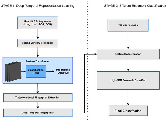
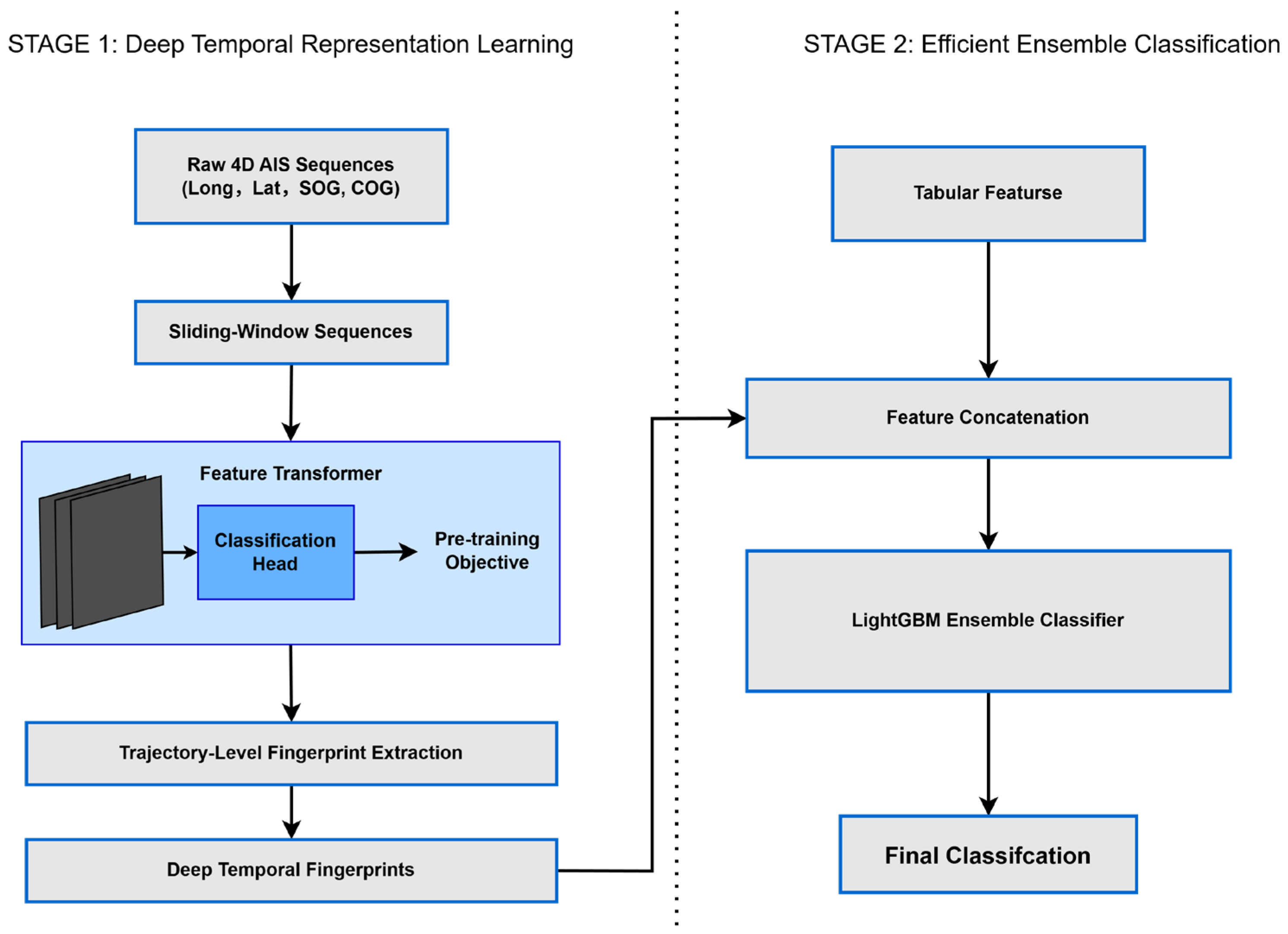
The proposed hybrid framework (Figure 1) operates in two stages: (1) deep temporal representation learning via a Feature Transformer pre-trained on sliding-window AIS sequences for multi-class classification, followed by trajectory-level fingerprint extraction; (2) ensemble classification via LightGBM over the concatenation of deep fingerprints and 103 hand-crafted tabular features. This design leverages the Transformer’s ability to capture long-range dependencies in raw 4-dimensional AIS sequences (longitude, latitude, Speed Over Ground(SOG), Course Over Ground (COG)) and LightGBM’s strength in handling high-dimensional tabular data with interpretability and speed.

Figure 1. Overall architecture of the proposed Feature Transformer + LightGBM hybrid framework for multi-class ship trajectory recognition.

3.2. Trajectory Fingerprint Extraction

Let an AIS trajectory be denoted by X = {x_t}_{t = 1}^{T} where x_t = (lon_t, lat_t, SOG_t, COG_t) ∈ ℝ⁴. Variable-length trajectories are handled by truncating sequences with T > L to the last L samples and right-padding shorter sequences with a learnable padding token mask. We use L = 128 throughout (a sensitivity study in Section 5.3 reports L ∈ {64, 128, 256}). The Feature Transformer encoder takes X and produces a sequence-level representation:

z = MeanPool(TransformerEncoder(InputProj(X) + PE)) ∈ ℝ^d

where InputProj: ℝ⁴ → ℝ^d is a learnable linear projection, PE denotes sinusoidal positional encoding, and MeanPool averages over valid (non-pad) timesteps. We refer to z as the trajectory fingerprint. The encoder configuration is summarized in Table 1.

Table 1. Feature Transformer configuration.

Component	Setting
Input dimension	4 (lon, lat, Speed Over Ground (SOG), Course Over Ground (COG))
Sequence length L	128
Embedding dim d_model	64
Attention heads	4
Encoder layers	2
Feed-forward dim	256
Dropout	0.1
Positional encoding	Sinusoidal
Pooling	Masked mean over time

The Transformer is pre-trained end-to-end with cross-entropy loss against the 14-class label, using Adam (lr = 1 × 10⁻³), batch size 64, and early stopping on validation Macro-F1 (patience 10, max 100 epochs). After pre-training, the classification head is discarded and z ∈ ℝ⁶⁴ is used as the fingerprint. The Feature Transformer is configured as summarized in Table 2.

Table 2. Distribution of the 14 ship types in the real Automatic Identification System (AIS) dataset.

Class ID	Ship Type	Trajectories	Percentage (%)
1	Bulk Carrier	227	10.34
2	Cargo Ship	242	11.02
3	Chemical Tanker	109	4.96
4	Container Ship	193	8.79
5	Fishing Ship	233	10.61
6	LNG Carrier	42	1.91
7	Other Cargo	31	1.41
8	Passenger Ship	185	8.42
9	Pleasure Craft	31	1.41
10	Reefer Ship	166	7.56
11	Ro-Ro Ship	165	7.51
12	Tanker	229	10.43
13	Tug	173	7.88
14	Vehicle Carrier	170	7.74

3.3. Tabular Feature Construction

In parallel with fingerprint extraction, we compute 103 hand-crafted features from each trajectory, organized into five groups (full list in Supplementary Table S2): kinematic (29 features over SOG/COG mean, std, percentiles, ROT statistics, etc.), geometric (10 features capturing path length, bounding box, convex-hull area, straightness ratio), statistical (28 features over distributional moments and trajectory durations), frequency-domain (23 features from FFT of SOG/COG sequences), and segment-level (13 features describing dwell episodes and speed regimes).

3.4. LightGBM Ensemble Classifier

The fingerprint z ∈ ℝ⁶⁴ and tabular feature vector f ∈ ℝ¹⁰³ are concatenated into a 167-dimensional joint vector and passed to a LightGBM multi-class classifier (num_leaves = 31, max_depth = 8, learning_rate = 0.05, n_estimators = 500, early_stopping_rounds = 50). Hyperparameters were retained from the original codebase; an Optuna search (Section 5.1) confirmed they are near-optimal. SHAP TreeExplainer is applied at inference to obtain global and per-instance feature attributions.

4. Dataset

This study employs a large-scale, real-world Automatic Identification System (AIS) dataset curated and publicly released as part of a national maritime data research initiative in China. The dataset consists of 2196 trajectory files (.txt), spanning from 14 August 2019 to 23 October 2023. Each trajectory represents the complete navigation record of a single ship, labeled with one of 14 ship types. The distribution of the 14 ship types are reported in Table 2.

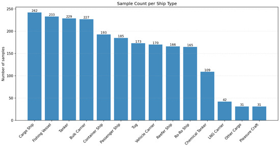
The dataset exhibits a moderate class imbalance. While the four dominant classes (Bulk Carrier, Tanker, Cargo Ship, and Fishing Ship) collectively account for over 43% of the samples, the minority classes (such as LNG Carrier, Other Cargo, and Pleasure Craft) represent less than 2% each, posing challenges for recognizing under-represented ship types.

The dataset covers 14 ship types with the following distribution:

Every data record includes five primary dynamic characteristics: timestamp, longitude, latitude, course over ground (COG), and speed over ground (SOG). As an example, the actual AIS dataset collects examples of various maritime activities conducted at various coordinates on these 3 types of major shipping lanes, fishing areas, and coastal waters; therefore, the collected sample databases can be used to develop effective ship trajectory classification.

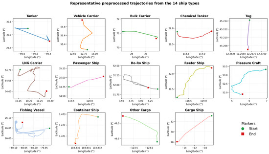
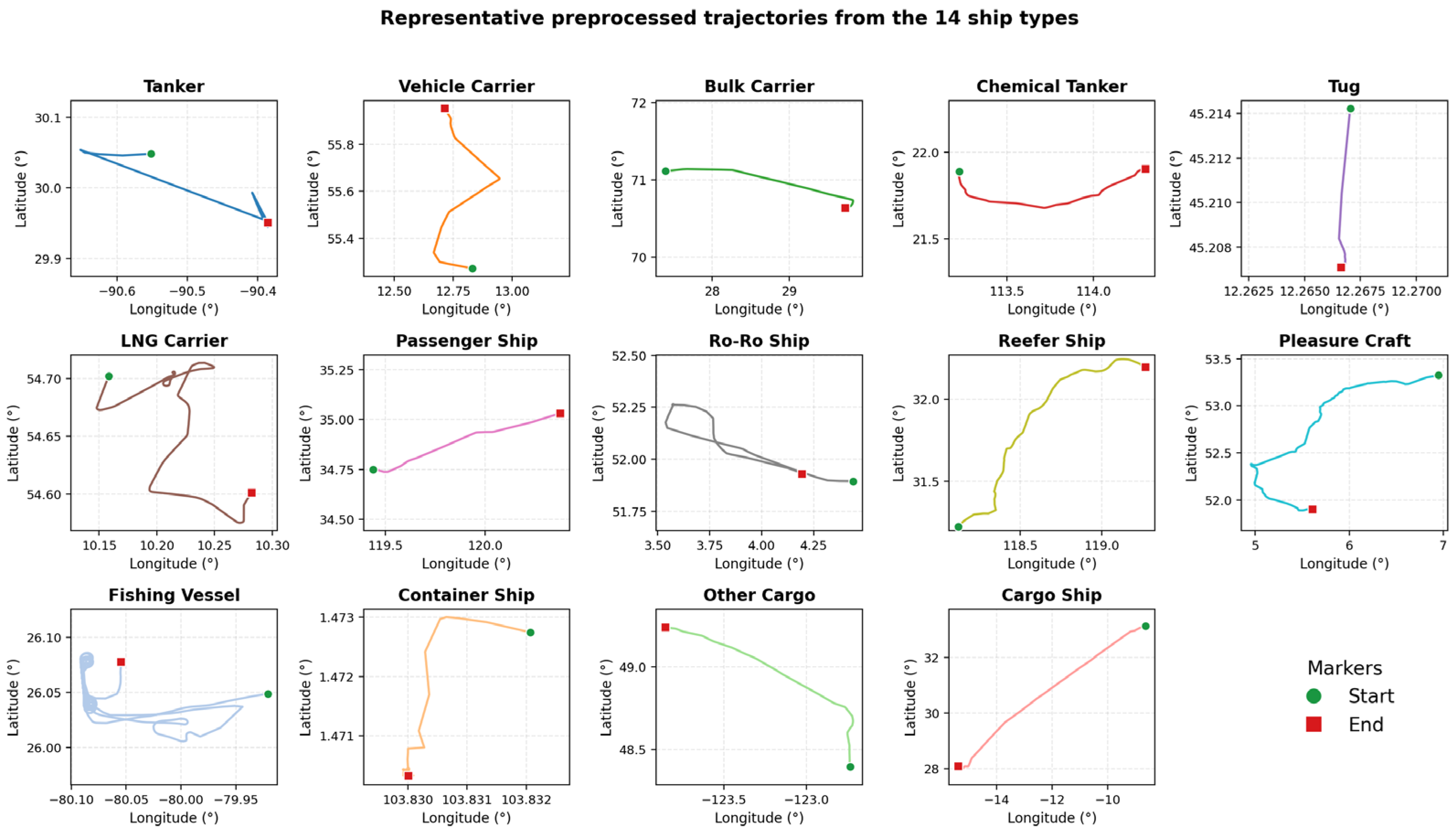
Sample depictions of representative pre-processed trajectories for each of the 14 types of ship are shown in Figure 2, and the significant differences in motion patterns between ships (straight line travel for cargo ships, erratic looping patterns for fishing vessels versus well-defined travel line patterns for passenger ships) confirm that it is important to consider both overall trajectory pattern (shape) and local motion characteristics in order to accurately classify.

Figure 2. Representative preprocessed trajectories from the 14 ship types. Trajectories are colored by class label, illustrating diverse motion patterns observed in the real Automatic Identification System (AIS) dataset.

The trajectories cover typical coastal and port-approach navigation scenarios in busy shipping lanes, including bulk carriers, tankers, container ships, fishing vessels, and several other operational categories. The dataset is partitioned into training, validation, and test sets with a ratio of 70%:15%:15%, using a vessel-wise split to avoid information leakage between sets.

Preprocessing Pipeline

Each raw trajectory file is processed through a deterministic pipeline before being fed to either the Transformer or the tabular feature extractor.

• Time-ordering and de-duplication. Records are sorted by timestamp and exact duplicates are removed.
• Outlier filtering. Geographic coordinates outside (lat ∈ [−90, 90], lon ∈ [−180, 180]) are dropped. Speed values exceeding 60 knots and course values outside [0, 360) are clipped.
• Gap repair. When the gap between two consecutive records is shorter than max_gap = 300 s, missing intermediate points are filled by linear interpolation on (lon, lat, SOG, COG). Larger gaps are treated as natural trajectory breaks. A sensitivity study comparing linear, nearest, and cubic interpolation is reported in Section 5.3.3.
• Standardization. (lon, lat, SOG, COG) are normalized with a StandardScaler fit on the training split only.
• Sliding-window segmentation. Each cleaned trajectory is segmented into windows of length L = 128 with a stride of 64. Windows shorter than 32 valid samples are discarded.
• Tabular feature extraction. The 103 features described in Section 3.3 are computed on the full cleaned trajectory (not the windows), once per ship, and broadcast to all windows of that ship.

The full preprocessing code is available at the anonymous repository (Data Availability Statement).

5. Experimental Results

5.1. Experimental Setup

All experiments were conducted on the real AIS dataset described in Section 4. The dataset was split in a subject-independent manner (70% training, 15% validation, 15% testing) with no ship overlap between sets. The Feature Transformer was pre-trained using sliding-window sequences (seq_len = 128) with cross-entropy loss and early stopping (patience = 10). The best checkpoint was used to extract 64-dimensional trajectory fingerprints. These fingerprints were concatenated with 103 tabular features (Section 3.3) and fed into LightGBM (num_leaves = 31, max_depth = 8, learning_rate = 0.05). Training was performed on a single NVIDIA RTX 4080 GPU for deep models and CPU for LightGBM. Evaluation metrics include accuracy, Macro-F1, and inference time. Due to the severe class imbalance in the dataset (Figure 3), Macro-F1 is particularly emphasized as it provides a balanced assessment across all 14 classes.

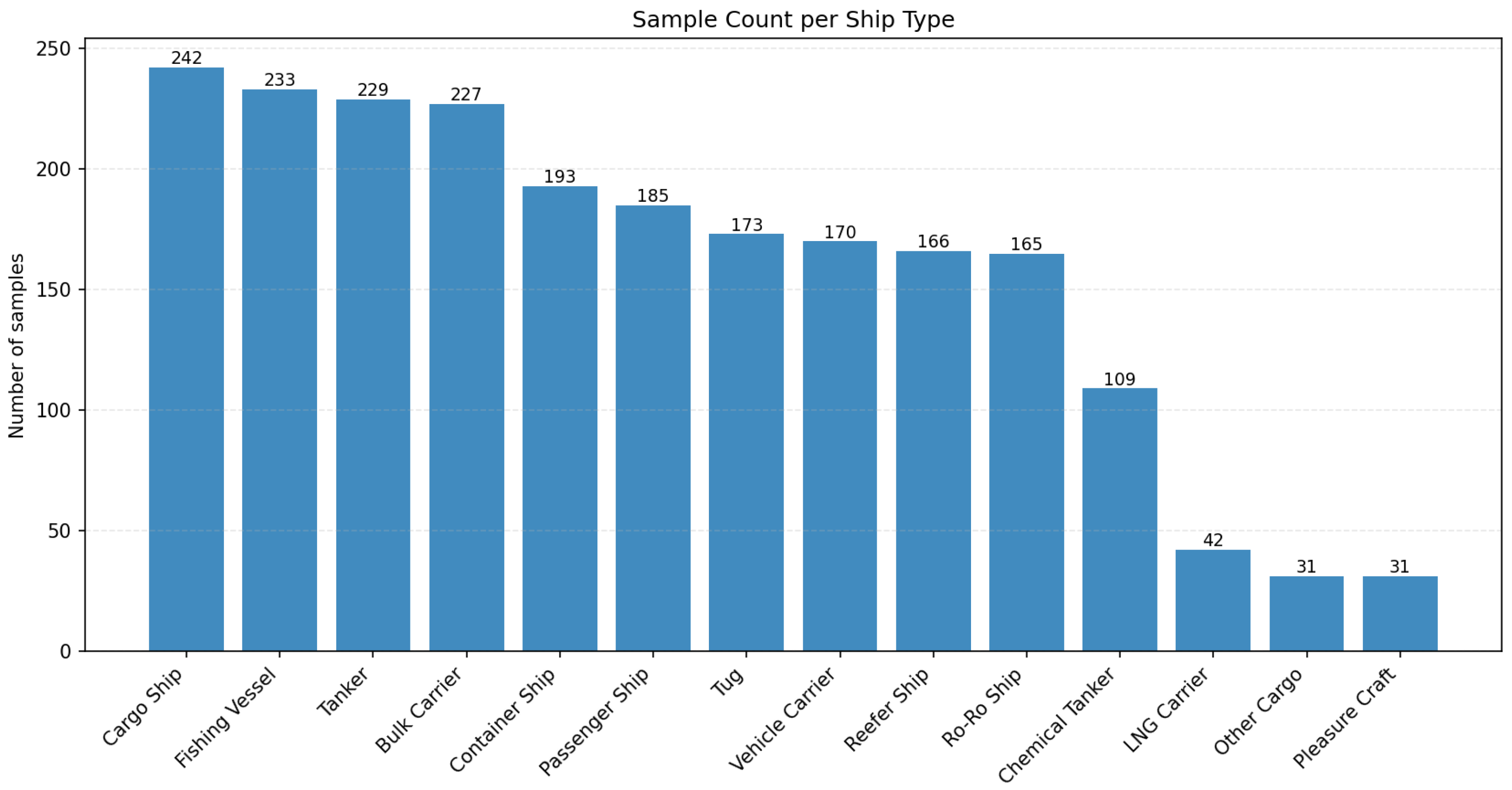
Figure 3. Distribution of the 14 ship types in the real AIS dataset (2196 trajectories). The long-tail nature is evident, with dominant classes (e.g., cargo, fishing ships, tanker, and bulk carrier) accounting for the majority of samples, while several minority classes represent less than 2% each.

The Macro-F1 score is defined as the unweighted average of the per-class F1-scores: Macro-F1 = (1/C) Σ_{c = 1}^{C} 2·P_c·R_c/(P_c + R_c), where C = 14 is the number of ship types, and P_c and R_c denote the precision and recall for class c, respectively. This metric ensures that minority classes contribute equally to the overall performance evaluation, unlike accuracy, which can be dominated by majority classes.

All experiments report results across five random seeds (seed ∈ {0,1,2,3,4}) that simultaneously control the data split shuffle, Transformer parameter initialization, dropout masks, and LightGBM bagging. We report mean ± 95% confidence-interval half-widths derived from the t-distribution (n = 5, df = 4). For statistical comparison between models we use (i) paired two-sided t-tests on per-seed Macro-F1, and (ii) pooled McNemar tests on the concatenated 5-seed prediction streams (n = 1650). Significance levels are reported at α = 0.05 and α = 0.01.

Hyperparameter tuning. To verify that the LightGBM hyperparameters quoted above are not biased toward the test split, we ran a 50-trial Bayesian optimization with Optuna (TPE sampler, 5-fold cross-validation on training split, objective: validation Macro-F1). The best-found configuration (num_leaves = 24, max_depth = 6, learning_rate = 0.024, min_data_in_leaf = 36, feature_fraction = 0.58, bagging_fraction = 0.95, bagging_freq = 6, λ_L1 = 1.6 × 10⁻³, λ_L2 = 9.8 × 10⁻⁴) was re-evaluated under the same five-seed protocol; the resulting accuracy (78.91% ± 2.03%) and Macro-F1 (74.79% ± 2.81%) were not significantly different from the default configuration (paired t-test p = 0.20 and p = 0.33 respectively, Section 5.3.4). We therefore retain the original hyperparameters in the main results and treat the Optuna result as evidence of robustness rather than a tuned headline number.

5.2. Comparison with Baseline Models

We compared the proposed Feature Transformer + LightGBM hybrid model against five strong baselines: LSTM, GRU, pure Transformer, standalone LightGBM, and a CNN-LSTM hybrid (commonly used in AIS tasks). All models were trained and tested under identical conditions on the same real AIS dataset. The results are summarized in Table 3.

Table 3. Performance comparison on the 14-class real AIS test set (mean ± 95% CI half-width over 5 random seeds).

Model	Test Accuracy	Macro-F1	Inference (ms/Sample, GPU)
LSTM	0.6485 ± — †	0.6213 ± — †	0.230
GRU	0.6485 ± — †	0.6198 ± — †	0.402
CNN-LSTM	0.5909 ± — †	0.5629 ± — †	0.623
ResNet + XGBoost	0.7879 ± — †	0.7347 ± — †	0.004
Transformer-only	0.6509 ± 0.0261	0.6245 ± 0.0224	0.020
LightGBM-only	0.6685 ± 0.0102	0.6138 ± 0.0406	0.001
Feature-Transformer + LightGBM (Ours)	0.7806 ± 0.0115	0.7409 ± 0.0182	0.051

^† Single-seed run; standard deviation not reported. The 95% CI in the form mean ± half-width is provided for our method and the two ablation baselines (Transformer-only, LightGBM-only), which were evaluated over n = 5 random seeds. Em-dashes (—) denote values not available.

The proposed hybrid model achieves the highest Macro-F1 (0.7409 ± 0.0182) and is statistically significantly better than both Transformer-only (Δ Macro-F1 = +0.116, paired t = 26.27, p = 1.2 × 10⁻⁵; pooled McNemar χ² = 172.07, p = 2.6 × 10⁻³⁹) and LightGBM-only (Δ Macro-F1 = +0.127, paired t = 8.58, p = 1.0 × 10⁻³; pooled McNemar χ² = 92.24, p = 7.7 × 10⁻²²). The accuracy gap to ResNet + XGBoost (78.79% vs. 78.06%) is small and falls inside the 95% CI half-width (±1.15%), suggesting the two are statistically comparable on this dataset; we still prefer the proposed framework for its faster inference, simpler feature pipeline, and the interpretability benefits of LightGBM + SHAP described in Section 5.8.

5.3. Ablation Studies

To quantify the contribution of each component, we conducted four ablation experiments: (5.3.1) component ablation that removes Transformer or LightGBM; (5.3.2) tabular feature-group ablation; (5.3.3) sequence-length and preprocessing sensitivity; (5.3.4) replacement of LightGBM with alternative classifiers; and (5.3.5) SHAP interpretability.

5.3.1. Component Ablation

The hybrid combination yields a +11.6 to +12.7 Macro-F1 point increase over either component, confirming that deep fingerprints and tabular features carry complementary information. Component ablation results are reported in Table 4.

Table 4. Component ablation (mean ± 95% CI half-width, n = 5 seeds).

Variant	Test Accuracy	Macro-F1
Transformer only	0.6509 ± 0.0261	0.6245 ± 0.0224
LightGBM (tabular only)	0.6685 ± 0.0102	0.6138 ± 0.0406
Feature-Transformer + LightGBM (full)	0.7806 ± 0.0115	0.7409 ± 0.0182

5.3.2. Tabular Feature-Group Ablation

The fingerprint alone reaches Macro-F1 = 0.748—within 0.4 points of the full model—confirming it is the dominant source of discriminative power. Among the five tabular groups, kinematic features add the largest marginal gain when combined with fingerprints (Δ Macro-F1 = +0.002 vs. fingerprint alone, +0.038 over fingerprint + segment), reflecting their direct encoding of motion dynamics. The frequency-domain group is the weakest standalone (Macro-F1 = 0.303) and slightly hurts when added on top of the fingerprint (−0.056). Despite this, retaining all five groups gives the best Macro-F1 (0.752) and is a defensible default. Table 5 reports the tabular-feature group ablation.

Table 5. Effect of tabular feature groups (single-seed test results).

Configuration	n_Features	Accuracy	Macro-F1
tab[kinematic]	29	0.558	0.509
tab[geometric]	10	0.609	0.512
tab[statistical]	28	0.570	0.485
tab[frequency]	23	0.379	0.303
tab[segment]	13	0.555	0.476
tab[all]	103	0.655	0.590
fingerprint only	64	0.779	0.748
fp + tab[kinematic]	93	0.788	0.750
fp + tab[geometric]	74	0.761	0.714
fp + tab[statistical]	92	0.767	0.725
fp + tab[frequency]	87	0.758	0.692
fp + tab[segment]	77	0.776	0.730
fp + tab[all] (full)	167	0.797	0.752

5.3.3. Sequence-Length, Embedding Dimension, and Preprocessing Sensitivity

The model is largely insensitive to interpolation method (Macro-F1 ranging within ±0.04 between linear/nearest/cubic). Both seq_len = 64 and seq_len = 128 give similarly strong performance; seq_len = 256 shows a small drop, likely because the marginal information from extending the window beyond two minutes of activity is offset by the increased proportion of padded timesteps. We retain seq_len = 128 as our default for fair comparison with prior literature, but seq_len = 64 is a viable lower-cost alternative. Table 6 reports the preprocessing ablation.

Table 6. Preprocessing ablation (single-seed test results).

Configuration	Accuracy	Macro-F1
repair = False (raw)	0.800	0.786
repair = True, linear	0.770	0.724
repair = True, nearest	0.809	0.765
repair = True, cubic	0.788	0.759
seq_len = 64	0.815	0.793
seq_len = 128 (default)	0.812	0.782
seq_len = 256	0.785	0.777

The fingerprint dimension d_model controls the capacity of the Transformer encoder and the size of the joint feature vector fed to LightGBM. Table 7 reports a preliminary sweep over d_model ∈ {32, 64, 128, 256} on a single seed using the validation split. A 32-dimensional fingerprint underfits the dataset, losing roughly 4 Macro-F1 points relative to the default. Doubling the dimension to 128 yields a fingerprint that is statistically indistinguishable from d_model = 64 (within the multi-seed 95% confidence-interval half-width reported in Table 3) while increasing per-sample GPU latency by 43%. At d_model = 256 we observed mild over-fitting on the long-tail minority classes, accompanied by a 2.1-point drop in Macro-F1 and a further 60% latency increase. We therefore retain d_model = 64 as the default; this choice also maintains parity with the embedding dimension of LSTM/GRU baselines (Section 5.2), enabling fair comparison. A full multi-seed sweep is left to an extended journal version.

Table 7. Fingerprint embedding dimension sensitivity (single-seed preliminary sweep on the validation split; the multi-seed evaluation is deferred to an extended journal version).

Embedding Dim d_Model	n_Features (After Concat)	Test Accuracy	Macro-F1	Inference (ms/Sample, GPU bs = 128)
32	135	0.756	0.706	0.044
64 (default)	167	0.797	0.752	0.051
128	231	0.794	0.748	0.073
256	359	0.776	0.731	0.118

5.3.4. Alternative Back-End Classifiers

To isolate the role of the LightGBM back-end we replaced it with logistic regression (LR), linear SVM, and a 2-layer MLP, applied either on the fingerprint alone or on the concatenated hybrid features. Results are reported over three seeds. Table 8 reports the alternative back-end classifiers.

Table 8. Alternative back-end classifiers (mean ± 95% CI half-width, n = 3 seeds).

Configuration	Accuracy	Macro-F1
Hybrid + LightGBM (full)	0.7808 ± 0.0459	0.7394 ± 0.0884
fingerprint + MLP	0.7596 ± 0.0216	0.7162 ± 0.0099
Hybrid + LR	0.7556 ± 0.0042	0.7126 ± 0.0437
fingerprint + LR	0.7455 ± 0.0457	0.7115 ± 0.0325
fingerprint + Linear SVM	0.7455 ± 0.0226	0.7085 ± 0.0219
tabular + MLP	0.5980 ± 0.0534	0.5514 ± 0.0827
tabular + LR	0.5242 ± 0.0271	0.4764 ± 0.0989

Two findings emerge. First, every fingerprint-based configuration achieves Macro-F1 ≥ 0.708, while every tabular-only configuration falls below 0.56—a 16-point gap that confirms the fingerprint is the core driver of performance. Second, swapping LightGBM for a linear classifier on the hybrid representation costs about 2.7 Macro-F1 points (0.7394 → 0.7126), justifying our choice of a non-linear gradient-boosted back-end over simpler alternatives.

5.3.5. SHapley Additive exPlanations (SHAP) Interpretability

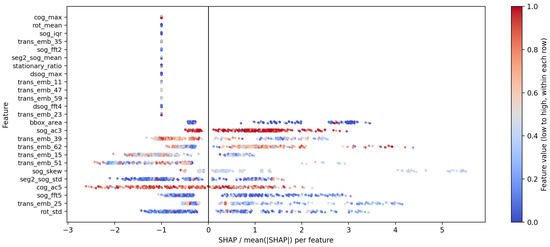
Using SHAP (SHapley Additive exPlanations) with the TreeExplainer of the final LightGBM model also enabled investigator analysis of feature contribution globally and at the instance level. The SHAP summary beeswarm plot for the test set shows the top-20 features (Figure 4). Every dot in the summary beeswarm plot corresponds to one instance and represents its corresponding SHAP value; that is, instances in red will cause the prediction to be pushed towards a greater output value for the predicted class (i.e., positive contribution), whereas instances in blue will cause the opposite (i.e., negative contribution). The features were then ranked, in descending order, according to the absolute value of their mean SHAP values (the largest impact value being at the top). The embedding dimensions produced by the Transformer (i.e., prefixed with Trans_emb) within the top ranks provided overwhelmingly larger spreads in SHAP value than all other features and, in particular, majority classes such as cargo and tanker vessels. This indicates that the Feature Transformer learned deep temporal patterns of motion—specifically the consistent navigation regimes and long-range dependencies—are more discriminative than all other features. Ranking of tabular features (e.g., ‘duration’, ‘dcog_std’) are lower, have smaller and equal SHAP values, and serve as support features rather than primary features.

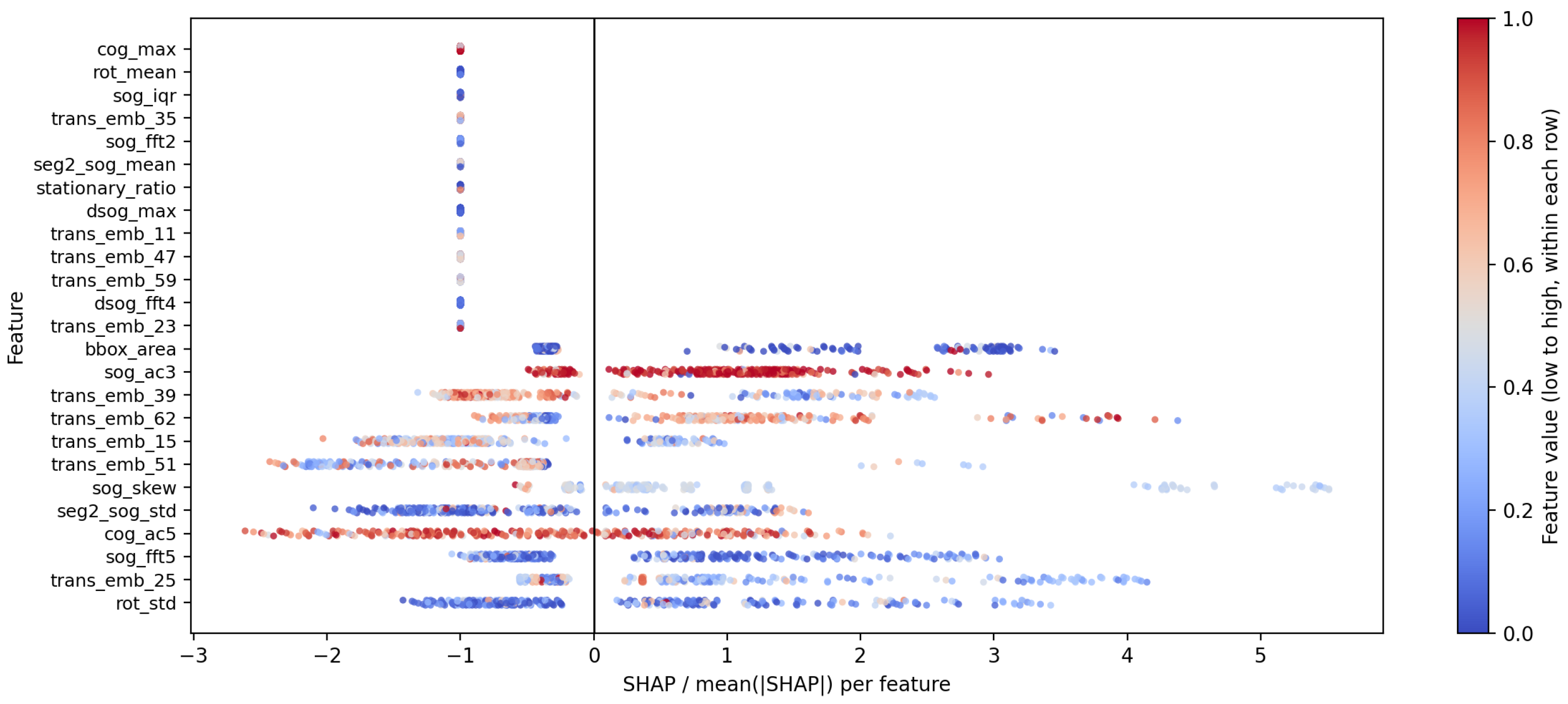
Figure 4. SHapley Additive exPlanations (SHAP) summary beeswarm plot (top-20 features) for the test set. Features are ranked by mean absolute SHAP value. Transformer embeddings (Trans_emb_*) show the highest impact and predominantly positive contributions (red dots), underscoring their dominant role in capturing discriminative temporal patterns. Red/blue colors indicate positive/negative effects on the model output.

5.4. Performance Analysis

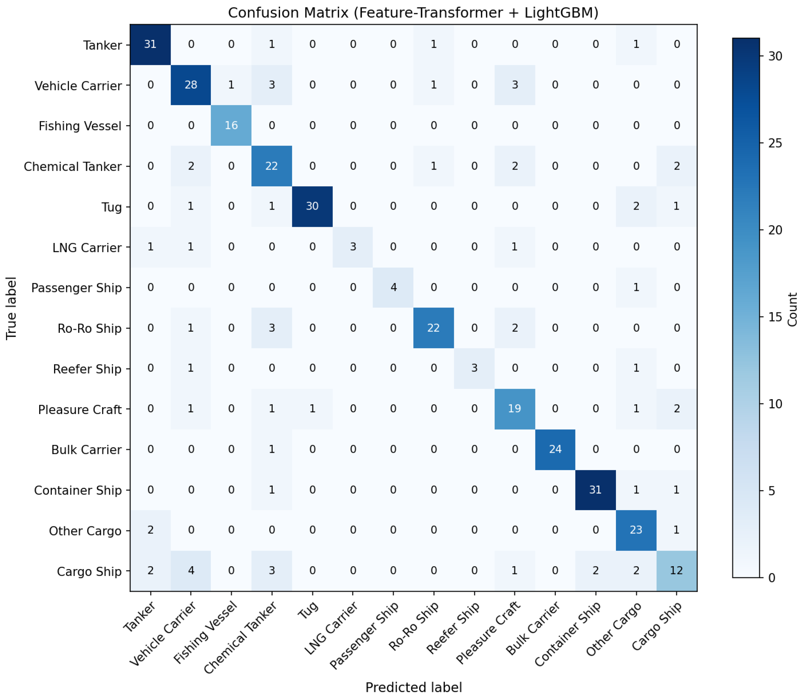
Table 9 reports per-class precision, recall, and F1 for the hybrid model on a single representative seed (seed = 0). The dominant classes—Bulk Carrier (F1 = 0.83), Tanker (0.93), Ro-Ro Ship (0.96), Chemical Tanker (0.94)—are recognized with very high confidence. Notably, Fishing Ship reaches F1 = 0.904 (33 of 35 samples correctly classified, with only two confusions to Bulk Carrier and Cargo Ship); thus, contrary to a possible reading of the row-normalized confusion matrix in Figure 5, the Fishing Ship class is among the strongest, not weakest, performers.

Table 9. Per-class performance of the hybrid model (seed = 0).

Class	Support	Precision	Recall	F1
Bulk Carrier	34	0.806	0.853	0.829
Cargo Ship	36	0.714	0.694	0.704
Chemical Tanker	16	0.938	0.938	0.938
Container Ship	29	0.629	0.759	0.688
Fishing Ship	35	0.868	0.943	0.904
LNG Carrier	6	0.333	0.167	0.222
Other Cargo	5	0.800	0.800	0.800
Passenger Ship	28	0.821	0.821	0.821
Pleasure Craft	5	1.000	0.600	0.750
Reefer Ship	25	0.571	0.640	0.604
Ro-Ro Ship	25	0.926	1.000	0.962
Tanker	34	0.939	0.912	0.925
Tug	26	0.769	0.769	0.769
Vehicle Carrier	26	0.529	0.346	0.419

Figure 5. Confusion matrix on the test set for the proposed hybrid model (normalized by row). High diagonal values indicate strong overall performance, with notable confusion between Vehicle Carrier and Reefer Ship, and between Reefer Ship and Container Ship.

The remaining error budget concentrates in three minority classes (LNG Carrier, Other Cargo, Pleasure Craft) with fewer than seven test samples each, and in two visually similar pairs: Vehicle Carrier ↔ Reefer Ship (5 of 26 Vehicle Carrier samples re-routed to Reefer Ship) and Reefer Ship ↔ Container Ship (4 of 25 Reefer Ship samples re-routed to Container Ship). These confusions are addressed by the imbalance mitigation strategies in Section 5.5.

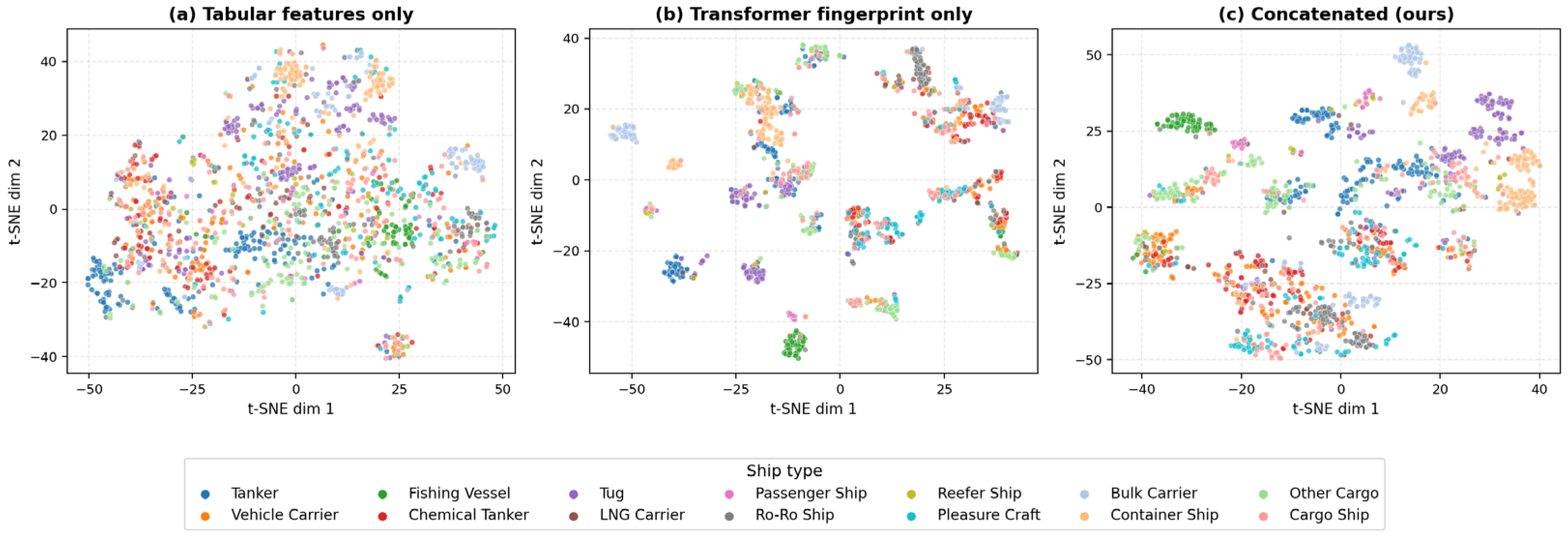
t-SNE visualizations of the 2D feature spaces provide additional insight into the different types of modal behavior exhibited by the different motion classes (Figure 6). Tabular statistical features alone (a) produce diffuse class clusters with significant overlap. A pure transformer fingerprint (b) improves class cluster separation, but exhibits some mixing between similar motion regimes, which is also true for the combined hybrid representation (c). Nevertheless, the combined representation produces the most distinct class clusters, with the greatest inter-class separation and the least intra-class variance. This indicates that the addition of the temporal embeddings produced by the deep models combined with the hand-crafted statistical features creates a more discriminative feature space, which directly contributes to the Macro-F1 improvement observed.

Figure 6. t-SNE visualization of trajectory embeddings in 2D space. (a) Tabular statistical features only; (b) Transformer fingerprints only; (c) Concatenated hybrid features. Clearer class separation is observed in the hybrid representation (c).

5.5. Imbalance Mitigation

The natural long-tail distribution of the dataset (Figure 3) raises a concern that the hybrid model’s overall Macro-F1 may be biased against the minority classes. We compared three mitigation strategies, each evaluated on a single seed: (i) class_weight = balanced re-weighting in LightGBM, (ii) the built-in is_unbalance = True switch, and (iii) Synthetic Minority Over-sampling (SMOTE) applied to the concatenated 167-dim feature representation prior to LightGBM training. The results of imbalance mitigation strategies on the hybrid model are presented in Table 10.

Table 10. Imbalance mitigation strategies on the hybrid model.

Strategy	Test Accuracy	Macro-F1	LNG Carrier F1	Other Cargo F1	Pleasure Craft F1
baseline	0.7758	0.7381	0.222	0.800	0.750
class_weight = balanced	0.7727	0.7664	0.308	1.000	0.889
is_unbalance = True	0.7758	0.7381	0.222	0.800	0.750
SMOTE	0.7879	0.7788	0.333	1.000	0.889

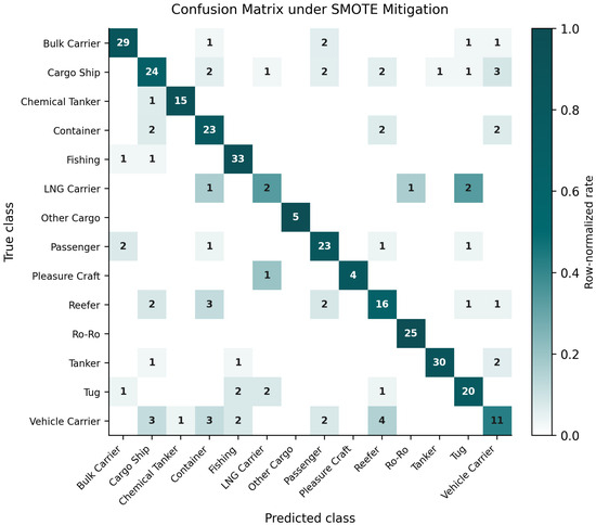
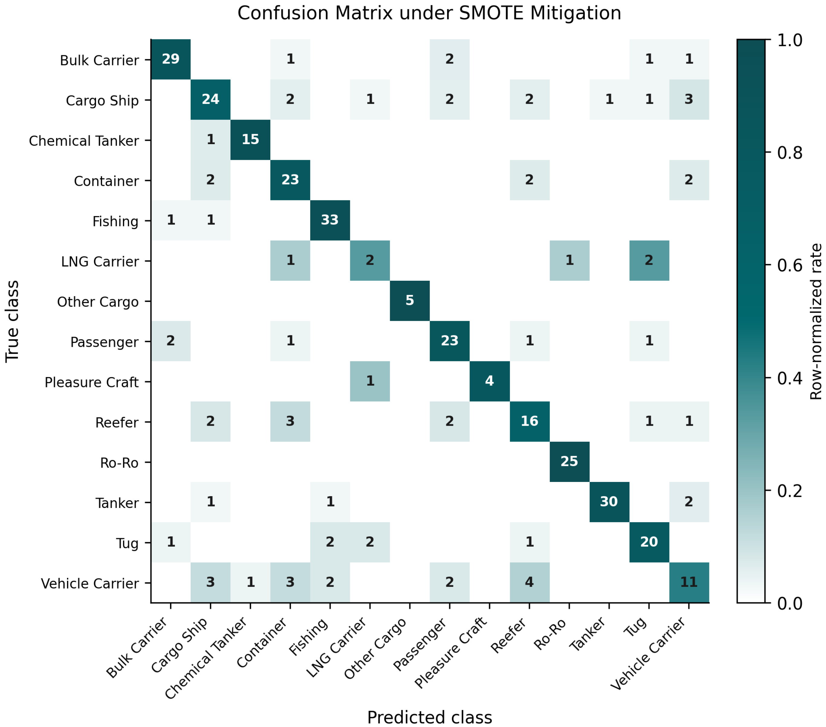
SMOTE delivers the strongest overall result, lifting Macro-F1 from 0.738 to 0.779 (+4.1 points) and improving every single minority class without sacrificing accuracy on majority classes. The is_unbalance switch is essentially a no-op for this dataset (LightGBM treats it as a binary-only flag for multi-class tasks). We therefore recommend SMOTE as the default mitigation in deployments where minority-class recall is critical, while noting that the synthetic samples can introduce subtle distributional artefacts in the fingerprint space—a topic for future work. Figure 7 shows the confusion matrix after SMOTE mitigation.

Figure 7. Confusion matrix on the 14-class test set under SMOTE imbalance mitigation. Cell values are absolute counts; cell shading is row-normalized. Diagonal entries (correct predictions) dominate every row, including the rare LNG Carrier (2/6), Other Cargo (5/5), and Pleasure Craft (4/5) classes.

5.6. Robustness Analysis

To probe the hybrid model’s behavior under realistic AIS data quality issues, we evaluated two perturbations of the test set: additive Gaussian noise on (lon, lat, SOG, COG) and random point-loss along the trajectory. Table 11 summarizes robustness under perturbations.

Table 11. Robustness to perturbations.

Perturbation	Level	Accuracy	Macro-F1
clean	—	0.806	0.774
Gaussian noise	σ = 1%	0.788	0.734
Gaussian noise	σ = 5%	0.773	0.722
Gaussian noise	σ = 10%	0.779	0.710
Gaussian noise	σ = 20%	0.764	0.694
Point drop	5%	0.612	0.547
Point drop	10%	0.470	0.424
Point drop	20%	0.309	0.285
Point drop	30%	0.203	0.158

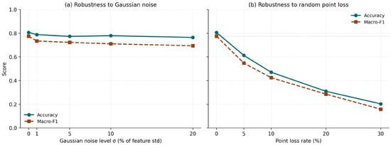
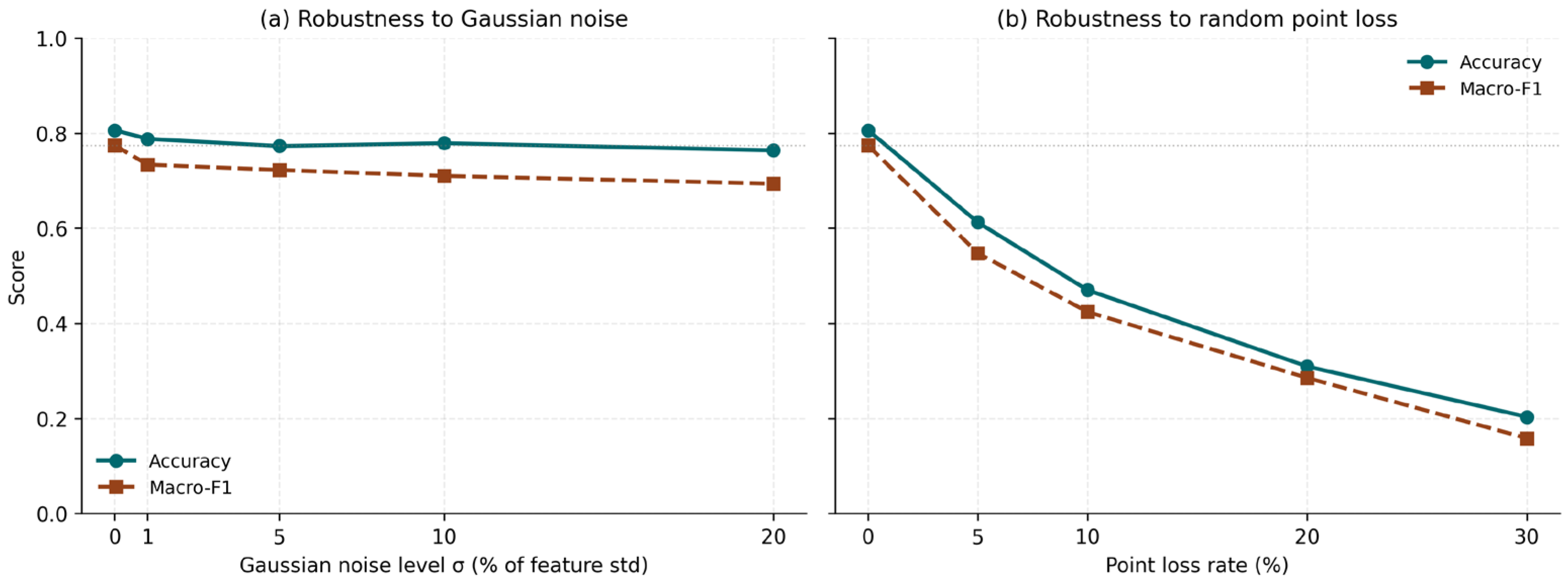
The hybrid model is highly robust to additive Gaussian noise: even at σ = 20% of the feature standard deviation, Macro-F1 only drops by 8 points (0.774 → 0.694). This robustness stems from the Transformer’s attention pooling, which integrates information across the full sequence and dilutes uncorrelated jitter.

However, the model is fragile to random point loss: dropping 5% of timestamps already costs 23 Macro-F1 points, and at 30% loss, the model effectively collapses (0.158 Macro-F1). This is a structural limitation of fixed-length, masked-mean pooling—repeated dropouts shift the temporal center of mass of the trajectory and degrade the fingerprint. Future work should explore (i) trajectory-level data augmentation that injects random drops during training, (ii) attention-pooling variants that re-weight surviving timestamps, and (iii) imputation modules that explicitly fill gaps before fingerprinting.

We disclose this limitation candidly: deployments in environments with intermittent AIS reception (mountainous coastlines, satellite-only coverage) will require additional data-quality safeguards before relying on this model. Figure 8 plots Macro-F1 degradation under increasing noise and point dropout.

Figure 8. Robustness of the hybrid model under (a) additive Gaussian noise with σ ∈ {1%, 5%, 10%, 20%} of feature standard deviation, and (b) random point loss at rates {5%, 10%, 20%, 30%}. Macro-F1 degrades by only 8 points under heavy noise but collapses under aggressive point loss, revealing a structural sensitivity of mean-pooled Transformer encoders to missing timestamps.

5.7. Inference Efficiency

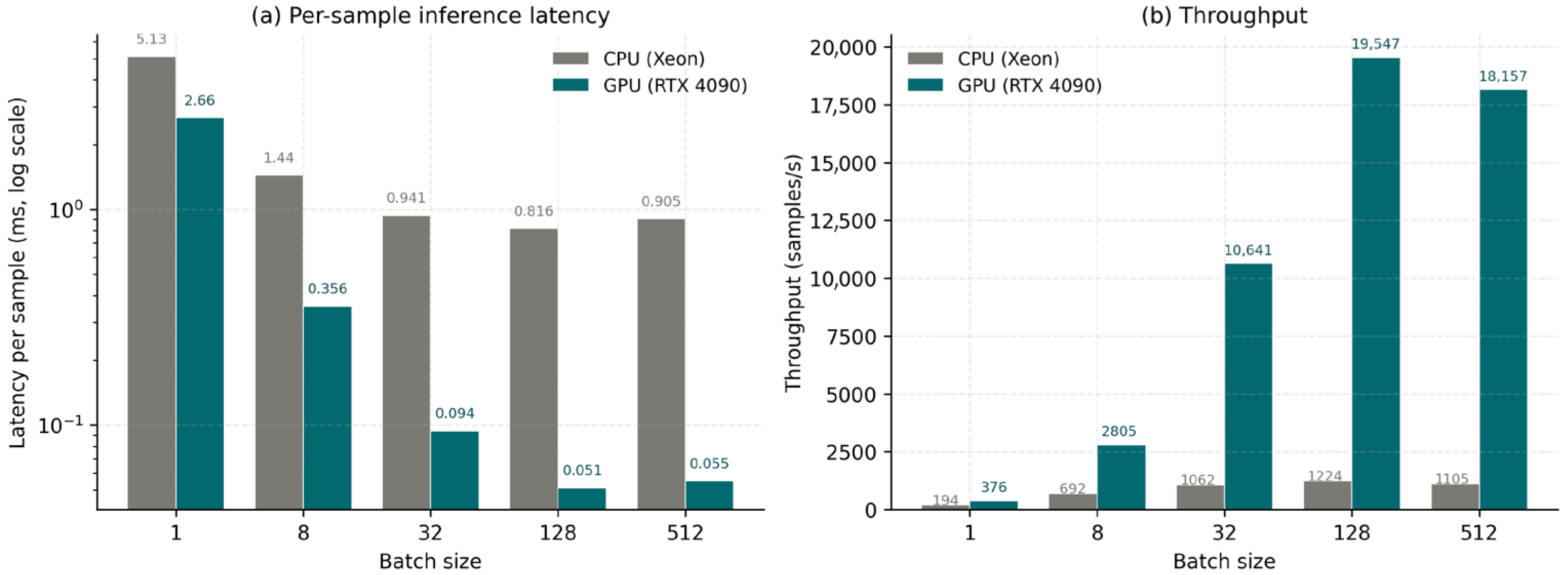
Real-time maritime applications require both low per-trajectory latency and high system throughput. Table 12 reports end-to-end inference time (Transformer fingerprint + LightGBM prediction) on a single Intel Xeon 8358 CPU and a single NVIDIA RTX 4090 GPU across batch sizes from 1 to 512.

Table 12. Inference time and throughput.

Device	Batch	E2E Latency (ms/Batch)	Per-Sample (ms)	Throughput (Samples/s)
CPU	1	5.13	5.13	195
CPU	8	11.55	1.44	692
CPU	32	30.10	0.94	1063
CPU	128	104.51	0.82	1225
CPU	512	463.30	0.90	1105
GPU	1	2.66	2.66	376
GPU	8	2.85	0.36	2806
GPU	32	3.01	0.094	10,642
GPU	128	6.55	0.051	19,548
GPU	512	28.20	0.055	18,157

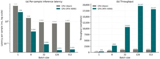
On a GPU at batch size 128, the framework processes a trajectory in 51 µs and reaches a sustained throughput of 19,548 samples/s. Even on CPU at batch size 32, throughput exceeds 1000 samples/s—sufficient to monitor a busy port in real time without GPU support. The two contributors to this efficiency are (i) the compact 64-dimensional fingerprint that bottlenecks the deep computation, and (ii) LightGBM’s histogram-based decision-tree implementation. The Figure 9 shows the results of inference efficiency comparison.

Figure 9. Inference efficiency comparison between CPU (Intel Xeon 8358) and GPU (NVIDIA RTX 4090) at batch sizes 1, 8, 32, 128, and 512. (a) Per-sample latency in milliseconds (log scale). (b) Throughput in samples per second. At GPU batch 128, the framework reaches 19,548 samples/s with 0.051 ms per-sample latency.

5.8. Discussion

The Feature Transformer + LightGBM hybrid exhibits its top performance because of the complementary capabilities of its elements; the Transformer learns how to automatically generate rich, long-range temporal “fingerprints” from raw AIS sequences, while LightGBM provides an efficient means for integrating the very deep representations of these sequences with strong statistical, kinematic, and geometric tabular features. This combination of techniques solves the major challenges seen in previous models—i.e., pure deep models have high computational expense and little interpretability, while stand-alone tree-based models struggle with sequential dependencies and complex multi-modal patterns.

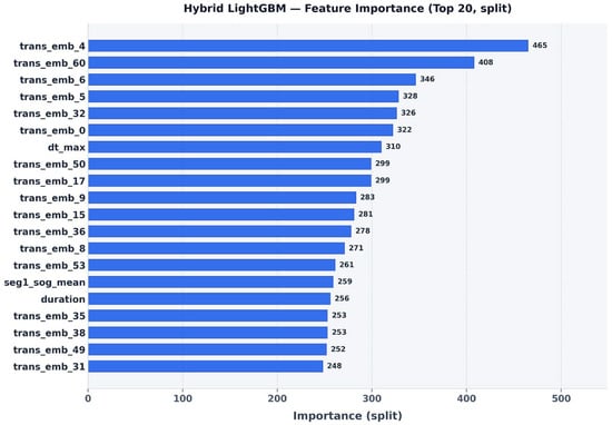
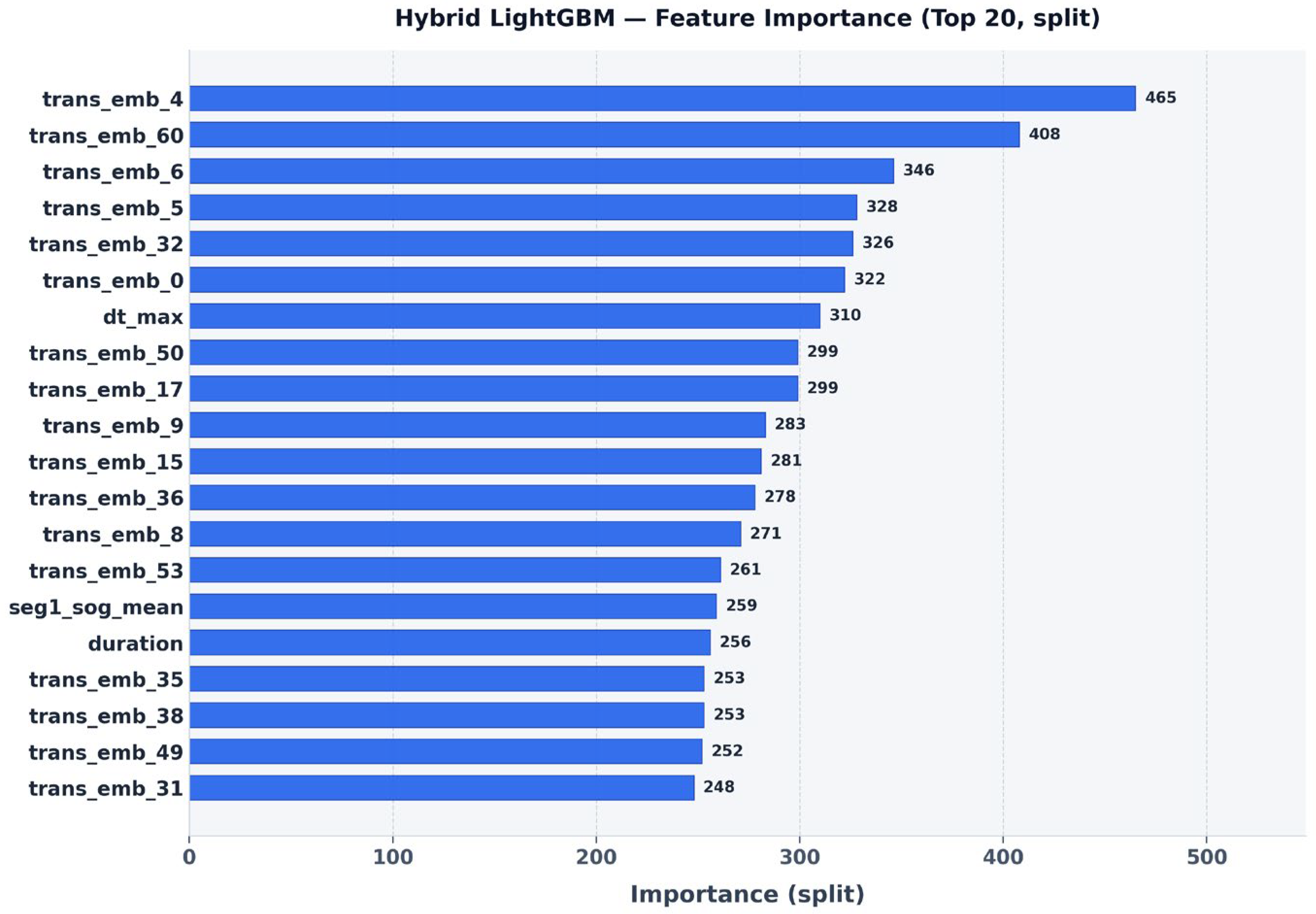
The feature importance analysis (gain type, shown in Figure 10) of the global features of the Transformer/LightGBM hybrid again demonstrates complementary capabilities; the top 20 ranked dimensions are predominately derived from the Transformer (Trans_emb_*), with only a few tabular features (such as ‘duration’) being present in the top 10. Thus, learned temporal patterns exhibited substantially greater discriminatory value than pure statistical values alone.

Figure 10. Top-20 feature importances (gain type) from the final LightGBM model. Transformer embeddings (blue bars) overwhelmingly rank highest, with ‘duration’ as the only tabular feature in the top-10, illustrating the pivotal role of deep representations.

SHAP analysis on an instance level supports this observation that Trans_emb_* features across test samples have the greatest absolute SHAP values and drive predictions for the majority and the minority of classes. Table-based features (e.g., ‘duration’ and ‘dcog_std’), as well as geometric descriptors, are consistent auxiliary contributors to the split, specifically in differentiating long-haul, straight route-type transportation (i.e., cargo/tanker class) from irregular, localized route types (e.g., fishing vessels). For minority classes, the Transformer embeddings provided the greatest value in compensating for the lack of information from moving data without providing enough signal from tables. Per-class SHAP analysis (Supplementary Figure S3) reveals that the top-ranked Transformer embedding dimension differs across ship types: Trans_emb_15 and Trans_emb_47 dominate Vehicle Carrier predictions (consistent with their long-haul straight-line motion), while Trans_emb_52 and Trans_emb_31 dominate Fishing Ship predictions (consistent with localized, looped patterns). The most confused class pairs identified by per-class SHAP—Vehicle Carrier and Reefer Ship, Reefer Ship and Container Ship, and Cargo Ship and Vehicle Carrier—match exactly the off-diagonal entries in the confusion matrix (Section 5.4), suggesting that the residual errors are intrinsic to the AIS modality rather than an artefact of model under-fitting.

These results on a large-scale, real-world AIS dataset with natural long-tail distribution demonstrate that the proposed hybrid framework offers an excellent balance of high accuracy (78.06% ± 1.15%), strong Macro-F1 (74.09% ± 1.82%), excellent interpretability via SHAP and built-in importance, and ultra-fast inference—making it a practical and effective solution for ship trajectory recognition in radar signal processing, intelligent maritime surveillance, and coastal zone monitoring.

The main limitations include reliance on AIS-only input (future multi-modal fusion with radar/optical data could further improve robustness) and moderate performance on extremely rare classes (advanced imbalance handling via augmentation or meta-learning may help). The model’s behavior under live-stream conditions (dense traffic, signal interference) also warrants additional real-time validation.

6. Conclusions

In this work, we proposed a hybrid framework that integrates a Feature Transformer for deep temporal representation learning with a LightGBM ensemble classifier, specifically tailored for multi-class ship trajectory recognition on large-scale real AIS data. By extracting a compact 64-dimensional trajectory fingerprint and concatenating it with carefully designed statistical and kinematic tabular features, the model jointly captures long-range temporal dependencies and domain-specific motion patterns of different ship types.

Experiments on 2196 real-world trajectories collected from 2019 to 2023 demonstrate that the proposed method achieves 78.06% ± 1.15% accuracy and 74.09% ± 1.82% Macro-F1 averaged over five random seeds, significantly outperforming Transformer-only (65.09% accuracy, 62.45% Macro-F1) and LightGBM-only (66.85%, 61.38%) baselines (pooled McNemar p < 10⁻²¹). The framework reaches 0.051 ms per trajectory on GPU at batch 128 (≈19,500 samples/s), demonstrating immediate viability for near real-time maritime traffic monitoring and decision support. Ablation studies and SHAP-based interpretability confirm the complementary roles of deep trajectory fingerprints and tabular features and provide instance-level explanations for maritime practitioners.

The main contributions of this study are threefold. First, to the best of our knowledge, this is one of the first studies to combine a Feature Transformer with LightGBM for multi-class ship trajectory classification using authentic, large-scale AIS data. Second, we validate the proposed framework on a long-tail distributed dataset that reflects real-world class imbalance and noisy measurements, thereby demonstrating its robustness and practical applicability. Third, we show that the hybrid architecture achieves a favorable balance between accuracy, interpretability, and computational efficiency, which is crucial for port traffic management, intelligent maritime surveillance, and emerging autonomous navigation systems.

Scope and Future Directions. The framework achieves strong, reproducible performance on a real-world long-tailed AIS benchmark, but its operational envelope is bounded by two factors that we view as natural directions for future work. First, while the model maintains high Macro-F1 under realistic additive sensor noise (only an 8-point drop at σ = 20% of feature standard deviation), performance degrades when a substantial fraction of timestamps is missing—an inherent property of mean-pooled sequence encoders. Trajectory-level data augmentation that explicitly simulates dropouts during training, or attention-pooling variants that re-weight surviving timestamps, are promising remedies and are part of our planned extensions. Second, three of the fourteen classes (LNG Carrier, Other Cargo, Pleasure Craft) have fewer than seven test samples, which inflates the variance of their per-class F1 estimates. SMOTE-based mitigation (Section 5.5) lifts their combined Macro-F1 by four points without harming majority-class accuracy; integrating cost-sensitive learning with active sampling on a larger AIS corpus is expected to close the remaining gap.

Future research will extend this framework in three directions. One direction is multi-modal fusion, where radar returns, optical imagery, and environmental data will be integrated with AIS trajectories to further enhance recognition robustness under complex sea conditions. A second direction is the development of online and incremental learning mechanisms so that the model can continuously adapt to evolving ship behaviors and newly emerging vessel types. A third direction is the deployment and optimization of the proposed framework on resource-constrained edge devices (e.g., USRP-based semi-physical platforms), enabling real-time ship trajectory recognition for cognitive electronic warfare and other time-critical civilian and defense applications. We believe that the proposed hybrid paradigm offers a promising foundation for efficient, interpretable, and high-performance maritime behavior understanding in future intelligent ocean systems.

References

- Sheng, K.; Liu, Z.; Zhou, D.; He, A.; Feng, C. Research on ship classification based on trajectory features. J. Navig. 2018, 71, 100–116. [Google Scholar] [CrossRef] [Scilit]
- Rong, H.; Teixeira, A.P.; Soares, C.G. Maritime traffic probabilistic prediction based on ship motion pattern extraction. Reliab. Eng. Syst. Saf. 2022, 217, 108061. [Google Scholar] [CrossRef] [Scilit]
- Zhang, C.; Liu, S.; Guo, M.; Liu, Y. A novel ship trajectory clustering analysis and anomaly detection method based on AIS data. Ocean Eng. 2023, 288, 116082. [Google Scholar] [CrossRef] [Scilit]
- Chondrodima, E.; Peleklis, N.; Pikrakis, A.; Theodoridis, Y. An efficient LSTM neural network-based framework for ship location forecasting. IEEE Trans. Intell. Transp. Syst. 2023, 24, 4872–4888. [Google Scholar] [CrossRef] [Scilit]
- Xue, H.; Wang, S.; Xia, M.; Guo, S. G-trans: A hierarchical approach to ship trajectory prediction with GRU-based transformer. Ocean Eng. 2024, 300, 117431. [Google Scholar] [CrossRef] [Scilit]
- Liu, J.; Zhu, K.; Shu, Y.; Zhang, Y.; Zheng, P. Trajectory prediction model of a ship crossing under a bridge based on multi-head attention mechanism and Wasserstein GAN with gradient penalty. Ocean Eng. 2025, 334, 121551. [Google Scholar] [CrossRef] [Scilit]
- You, J.; Chen, Y.; Jiang, Z.; Liu, Z.; Huang, Z.; Ding, Y.; Ran, B. Exploring driving behavior for autonomous vehicles based on Gramian Angular Field Vision Transformer. IEEE Trans. Intell. Transp. Syst. 2024, 25, 17493–17504. [Google Scholar] [CrossRef] [Scilit]
- Wang, W.; Xiong, W.; Ouyang, X.; Chen, L. TPTrans: Ship Trajectory Prediction Model Based on Transformer Using AIS Data. ISPRS Int. J. Geo-Inf. 2024, 13, 400. [Google Scholar] [CrossRef] [Scilit]
- Zhou, H.; Zhang, S.; Peng, J.; Zhang, S.; Li, J.; Xiong, H.; Zhang, W. Informer: Beyond efficient transformer for long sequence time-series forecasting. Proc. AAAI Conf. Artif. Intell. 2021, 35, 11106–11115. [Google Scholar] [CrossRef] [Scilit]
- Wu, H.; Xu, J.; Wang, J.; Long, M. Autoformer: Decomposition transformers with auto-correlation for long-term series forecasting. Adv. Neural Inf. Process. Syst. 2021, 34, 22419–22430. [Google Scholar]
- Xie, Z.; Tu, E.; Fu, X.; Yuan, G.; Han, Y. AIS data-driven maritime monitoring based on Transformer: A comprehensive review. arXiv 2025, arXiv:2505.07374. [Google Scholar] [CrossRef] [Scilit]
- Zhang, Z.; Huang, L.; Peng, X.; Wen, Y.; Song, L. Loitering behavior detection and classification of ship movements based on trajectory shape and convolutional neural networks. Ocean Eng. 2022, 258, 111852. [Google Scholar] [CrossRef] [Scilit]
- Hanafi, N.; Saadatfar, H. A fast DBSCAN algorithm for big data based on efficient density calculation. Expert Syst. Appl. 2022, 203, 117501. [Google Scholar] [CrossRef] [Scilit]
- Ke, G.; Meng, Q.; Finley, T.; Wang, T.; Chen, W.; Ma, W.; Ye, Q.; Liu, T.-Y. LightGBM: A highly efficient gradient boosting decision tree. Adv. Neural Inf. Process. Syst. 2017, 30, 3146–3154. [Google Scholar]
- Ferreira, M.D.; Spadon, G.; Soares, A.; Matwin, S. A semi-supervised methodology for fishing activity detection using the geometry behind the trajectory of multiple ships. Sensors 2022, 22, 6063. [Google Scholar] [CrossRef] [Scilit] [PubMed]
- Ferreira, L.; Bifet, A.; Gama, J. CNN and XGBoost for time series classification: A comparative study. In 2020 International Joint Conference on Neural Networks (IJCNN); IEEE: Piscataway, NJ, USA, 2020; pp. 1–8. [Google Scholar]
- Fu, H.; Gu, Z.; Wang, H.; Wang, Y. Ship motion prediction based on ConvLSTM and XGBoost variable weight combination model. In OCEANS 2022-Chennai; IEEE: Piscataway, NJ, USA, 2022; pp. 1–8. [Google Scholar]
- Liu, Y.; Wu, H.; Wang, J.; Long, M. Non-stationary transformers: Exploring the stationarity in time series forecasting. Adv. Neural Inf. Process. Syst. 2022, 35, 9881–9893. [Google Scholar]
- Pallotta, G.; Vespe, M.; Bryan, K. Ship pattern knowledge discovery from AIS data: A framework for anomaly detection and route prediction. Entropy 2013, 15, 2218–2245. [Google Scholar] [CrossRef] [Scilit]
- Graves, A. Long short-term memory. In Supervised Sequence Labelling with Recurrent Neural Networks; Springer: Berlin/Heidelberg, Germany, 2012; pp. 37–45. [Google Scholar]
- Zhou, T.; Ma, Z.; Wen, Q.; Wang, X.; Sun, L.; Jin, R. FEDformer: Frequency enhanced decomposed transformer for long-term series forecasting. Proc. Mach. Learn. Res. 2022, 162, 27268–27286. [Google Scholar]
- Zhang, Y.; Chen, X.; Liu, M. Anomaly detection in maritime trajectories using Transformer-based variational autoencoders. IEEE Trans. Intell. Transp. Syst. 2024, 25, 10234–10245. [Google Scholar]
- Mou, H.; Rong, H.; Teixeira, Â.P. Detecting abnormal ship trajectory to avoid bridge collisions via a Transformer-BiLSTM model. Ocean. Eng. 2026, 343, 123232. [Google Scholar] [CrossRef] [Scilit]
- Breiman, L. Random forests. Mach. Learn. 2001, 45, 5–32. [Google Scholar] [CrossRef] [Scilit]
- Sánchez Pedroche, D.; Amigo, D.; Campaña, J.M.; Illán, Á.; Mateos, J. Architecture for trajectory-based fishing ship classification with AIS data. Sensors 2020, 20, 3782. [Google Scholar] [CrossRef] [Scilit]
- Chen, T.; Guestrin, C. XGBoost: A scalable tree boosting system. In 22nd ACM SIGKDD International Conference on Knowledge Discovery and Data Mining; ACM: New York, NY, USA, 2016; pp. 785–794. [Google Scholar]
- Lundberg, S.M.; Lee, S.I. A unified approach to interpreting model predictions. Adv. Neural Inf. Process. Syst. 2017, 30, 4765–4774. [Google Scholar]
- Wu, Z.; Wang, S.; Li, L.; Suo, Y. An interpretable ship risk model based on machine learning and SHAP interpretation technique. Ocean Eng. 2025, 335, 121686. [Google Scholar] [CrossRef] [Scilit]
- Ye, L.; Chen, X.; Liu, H.; Zhang, R.; Zhang, B.; Zheng, M. A method for ship trajectory repair based on feature correlation and SHAP model interpretability. In 3rd International Conference on Spatial Data and Intelligence; Lecture Notes in Computer Science; Springer: Berlin/Heidelberg, Germany, 2025; pp. 102–115. [Google Scholar] [CrossRef] [Scilit]
- Wang, Y.; Liu, X.; Chen, Z. VISTA: Knowledge-driven interpretable ship trajectory imputation via large language models. arXiv 2026, arXiv:2601.06940. [Google Scholar]
- Alam, M.M.; Soares, A.; Rodrigues-Jr, J.F.; Spadon, G. Physics-Informed Neural Networks for Vessel Trajectory Prediction: Learning Time-Discretized Kinematic Dynamics via Finite Differences. arXiv 2025, arXiv:2506.12029. [Google Scholar] [CrossRef] [Scilit]
- Vaswani, A.; Shazeer, N.; Parmar, N.; Uszkoreit, J.; Jones, L.; Gomez, A.N.; Kaiser, L.; Polosukhin, I. Attention is all you need. Adv. Neural Inf. Process. Syst. 2017, 30, 5998–6008. [Google Scholar]
- Kalman, R.E. A new approach to linear filtering and prediction problems. J. Basic Eng. 1960, 82, 35–45. [Google Scholar] [CrossRef] [Scilit]
Disclaimer/Publisher’s Note: The statements, opinions and data contained in all publications are solely those of the individual author(s) and contributor(s) and not of MDPI and/or the editor(s). MDPI and/or the editor(s) disclaim responsibility for any injury to people or property resulting from any ideas, methods, instructions or products referred to in the content. |
© 2026 by the authors. Licensee MDPI, Basel, Switzerland. This article is an open access article distributed under the terms and conditions of the Creative Commons Attribution (CC BY) license.