


Abstract
Railway safety inspections, a critical component of modern transportation systems, face significant challenges from adverse weather conditions, like fog and rain, which degrade image quality and compromise inspection accuracy. To address this limitation, we propose a novel deep learning-based image dehazing algorithm optimized for outdoor railway environments. Our method integrates adaptive high-pass filtering and bilateral grid processing during the feature extraction phase to enhance detail preservation while maintaining computational efficiency. The framework uniquely combines RGB color channels with atmospheric brightness channels to disentangle environmental interference from critical structural information, ensuring balanced restoration across all spectral components. A dual-attention mechanism (channel and spatial attention modules) is incorporated during feature fusion to dynamically prioritize haze-relevant regions and suppress weather-induced artifacts. Comprehensive evaluations demonstrate the algorithm’s superior performance: On the SOTS-Outdoor benchmark, it achieves state-of-the-art PSNR (35.27) and SSIM (0.9869) scores. When tested on a specialized railway inspection dataset containing 12,840 fog-affected track images, the method attains a PSNR of 30.41 and SSIM of 0.9511, with the SSIM being marginally lower (0.0017) than DeHamer while outperforming other comparative methods in perceptual clarity. Quantitative and qualitative analyses confirm that our approach effectively restores critical infrastructure details obscured by atmospheric particles, improving defect detection accuracy by 18.6 percent compared to non-processed images in simulated inspection scenarios. This work establishes a robust solution for weather-resilient railway monitoring systems, demonstrating practical value for automated transportation safety applications.
1. Introduction
Railway safety inspection is an essential means of ensuring the safe operation of railways and the safety of passengers’ lives and property. Railway transportation carries a large number of passengers and goods, and in the event of an accident, it can cause severe casualties and property losses [1]. Real-time monitoring of railway safety is necessary. However, under adverse weather conditions, such as rain and fog, monitoring systems struggle to accurately detect issues like loose railway bolts and rail fractures [2]. This paper aims to address these challenges by proposing an efficient image dehazing method.
Image dehazing is an important computer vision technology, aiming to restore clear visual information from images affected by factors such as rain, fog, and insufficient lighting [3]. Derivative technologies of this technique are widely applied in fields such as medical imaging, safe driving, and video surveillance [4]. Early image dehazing methods mainly relied on traditional linear filters [5], such as mean filters and Gaussian filters. Although these methods are simple, their effectiveness is limited when dealing with complex blurring effects. In the early 21st century, Bayesian methods gained popularity in image dehazing by establishing probabilistic models for hazy images and introducing prior information to constrain the restoration process [6]. Physical model-based approaches, such as the dark channel prior method [7,8], can estimate the transmission map and atmospheric light to restore haze-free images, but they perform poorly when objects have similar colors to the atmospheric light or contain large uniform areas. Traditional methods generally suffer from limitations such as reliance on manual priors, insufficient capability to handle complex scenes, and a tendency to cause color distortion and edge information loss [9].
With the development of deep learning, convolutional neural networks (CNNs) have promoted the advancement of image dehazing technology [10,11,12,13]. DehazeNet [14] and its lightweight improvement LDNet [15] reduce computational resource requirements and outperform traditional methods, but their simple network structures lead to unsatisfactory performance under extreme haze and complex lighting conditions. AODNet [16] can be jointly trained with object detection models to improve detection accuracy for hazy images, yet it still needs improvement in handling extreme haze, complex lighting scenarios, and generalization capabilities. FFA-Net [17] introduces channel and pixel attention modules to process thick haze and detailed features while avoiding over-processing in light haze regions. However, the increased network depth weakens the influence of shallow features, potentially causing loss of image details. The DeHamer network [18], which combines the global modeling of Transformers with the local feature capabilities of CNNs [19,20], performs excellently in complex non-uniform haze scenarios, but its complex structure imposes higher computational demands and creates bottlenecks in computational resources.
Addressing issues such as inaccurate extraction of key details and insufficient multi-modal information fusion in railway scenarios for traditional and existing deep learning methods, this paper proposes a deep learning-based image dehazing method for large amounts of blurred and clear image data. In the image feature extraction stage, the AHFM module is introduced to simultaneously extract high-frequency and low-frequency filtering features and generate feature maps using an affine bilateral grid. An atmospheric luminance channel (A) is incorporated to help the network better restore color and edge information. In the feature fusion stage, the CBAM module is introduced to enhance the attention mechanism, highlighting important regions in the image. The feasibility and research value of the proposed method are validated through experiments.
The remaining sections of this study are organized as follows:Section 1 reviews previous research on deblurring tasks, Section 2 provides a detailed description of the proposed deblurring method, Section 3 describes the datasets used and presents experiments and analyses, and, finally, Section 4 summarizes the research findings.
2. The Overall Structural Framework
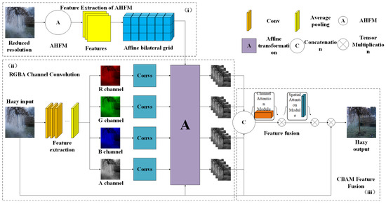
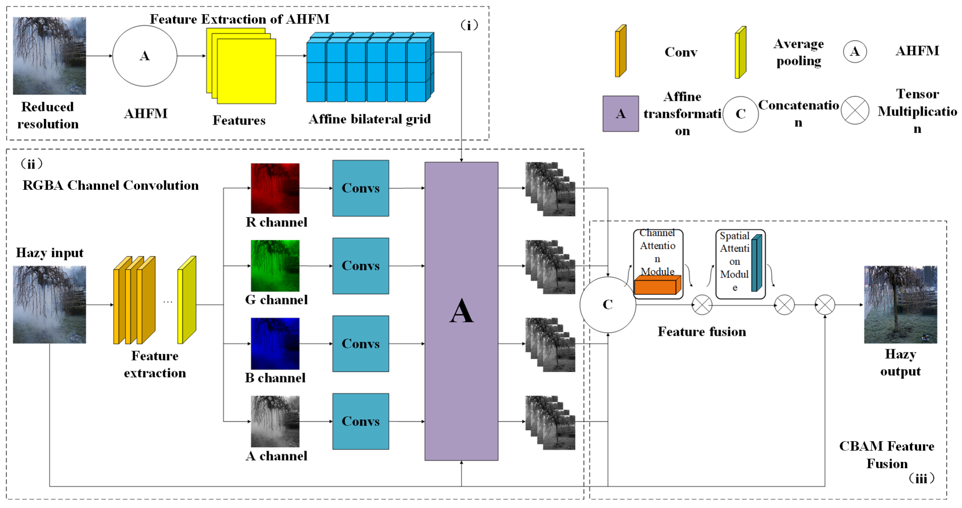
The overall algorithm framework of this paper is shown in Figure 1. The dehazing algorithm process is mainly divided into three modules: (a) feature extraction and bilateral grid application; (b) full-resolution feature reconstruction; and (c) CBAM feature fusion.
Figure 1.
Framework of research content.
Firstly, the hazy image is inputted and downsampled to a lower resolution through convolutional blocks and pooling layers, from which low-resolution features are extracted to compute the coefficients of the affine bilateral grid. Subsequently, affine bilateral grid learning is performed to capture local features and edge information of the image in the bilateral space using the grid. In the next module, the learned bilateral grid coefficients are utilized to upsample and interpolate the low-resolution features. Multiple guidance matrices are employed to extract guiding information from the RGBA channels, thereby reconstructing the feature maps. Finally, the features recovered from the guidance matrices and the bilateral grid are fused with the original high-resolution image features, and the dehazed output image is generated based on the fused features.
In this section, we will introduce the relevant algorithms for each module, as shown in Figure 1. The related experiments and analyses of the results will be presented in Section 2.
2.1. Feature Extraction and Application of Bilateral Grids
2.1.1. AHFM Feature Extraction
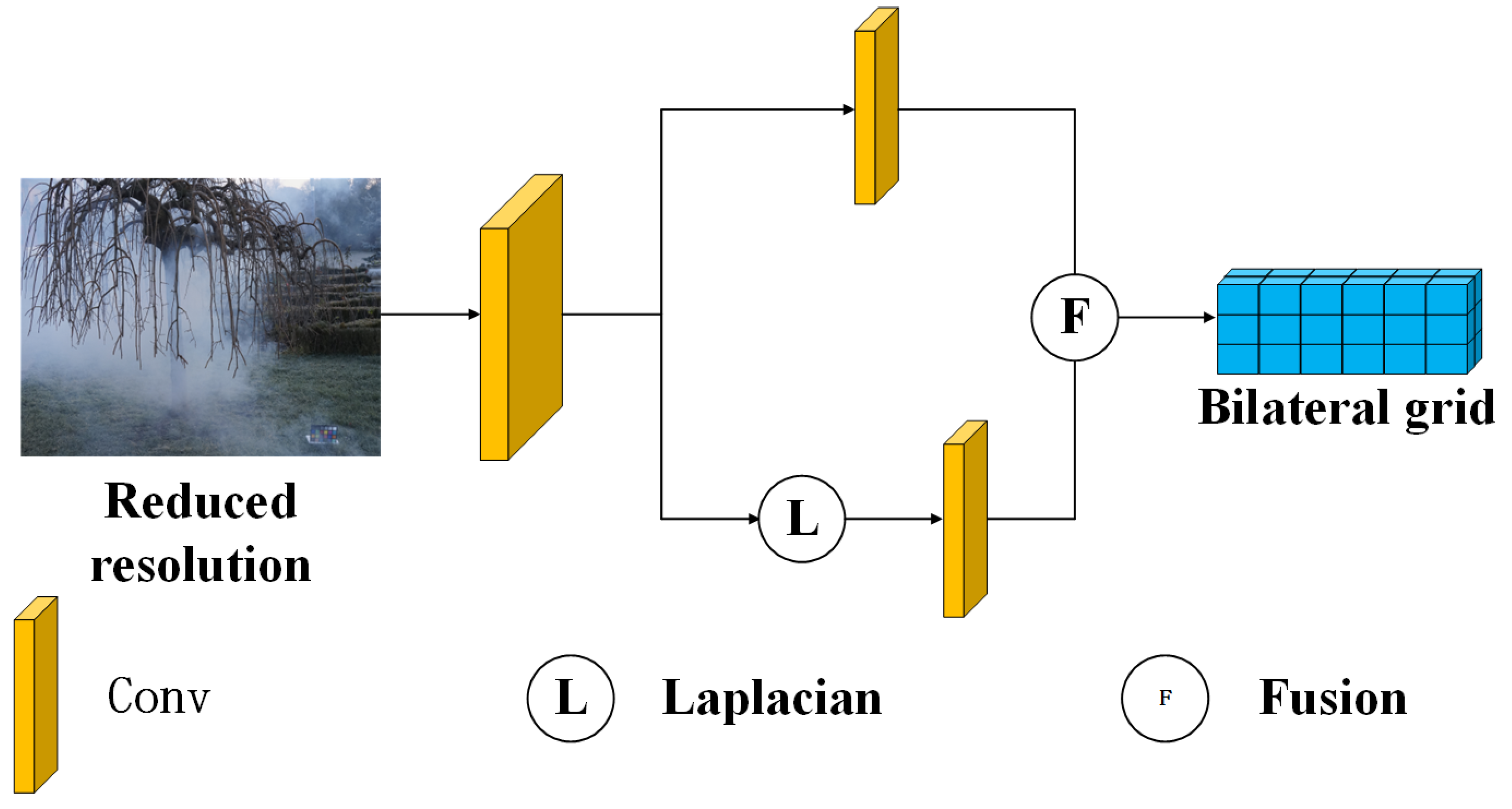
In this paper, we introduce an improved adaptive high-pass filtering module (AHFM), which uses a Laplacian filter to extract high-frequency information from the input feature maps, combining it with low-frequency information to enhance the model’s ability to capture details. The Laplacian filter has a lower computational cost, making it more efficient when applied to feature extraction [21].
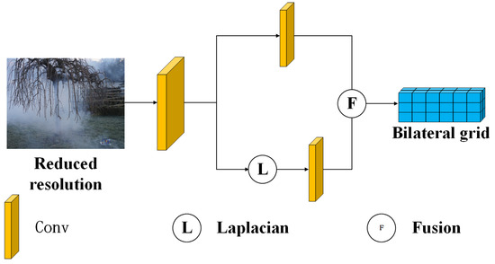
As shown in Figure 2, we first downsampled the 4K resolution blurry image to a fixed resolution of 910 × 512; then, we used standard convolutional operations to extract the initial feature maps P:
Figure 2.
Feature extraction of AHFM.
Among them, we have , where H, and C denote the height, width and number of channels of the feature map, respectively. In order to preserve the global low-frequency information, we then use a convolution operation to generate a smooth feature map :
We then extract the high-frequency feature maps using a Laplace filter with a standard 3 × 3 kernel of the Laplace filter as follows:
By filtering the initial feature map P, a high-frequency feature map can be obtained , as follows:
To enhance the important detail information, we process through an additional convolutional layer to optimize the extracted high-frequency information:
After obtaining the low-frequency features and high-frequency features, we fused them using weighted summation to generate the final feature map :
where and are learnable parameters that can be used to control the relative importance of low- and high-frequency information. At this point, we have completed the feature extraction operation, obtained the feature map , and used the following step of the operation.
2.1.2. Application of Bilateral Grids
In fogged images, the color and contrast between pixels are severely degraded, so it becomes especially important to recover the edges and details of the image. This problem can be better solved by the application of bilateral grids, which are able to learn the structure of fogged images by fitting an affine model [22]. After a feature extraction operation, we use the obtained feature map to learn an affine bilateral grid.
The bilateral grid is a three-dimensional array that takes into account the spatial information as well as the intensity information of the pixels, and each of its cells represents the coefficients of an affine transformation matrix for a particular region. This matrix is used to model the intensity ranges of different color channels, ensuring that pixels with different intensity ranges can be restored using different affine functions. This is a process that is formulated as
Among them, are the 3D coordinates of the bilateral grid, denotes the index of the grid in horizontal space, denotes the index in vertical space, denotes the index of the intensity dimension. are the coordinates in the feature map , x and y are the spatial positions of the image, and c is the color channel.
In this way, the affine transformation matrix in each grid cell is able to capture pixel features at different spatial locations and intensity ranges and personalize these pixels to enable better recovery of edges and details in the image.
2.2. Full-Resolution Feature Reconstruction
2.2.1. RGBA Color Channel
After the previous step, the model can learn some main information of the original image. However, if the image is compressed into a single guidance map for processing, it will lead to a large amount of color and detail information loss. In order to avoid this problem, we adopt the method of multi-guidance bilateral interpolation, i.e., we introduce four color channels, R, G, B, and A, which represent the general color channel and the atmospheric luminance channel, respectively, and we use them to generate the guidance matrix. In the standard RGB channel, the formula for each channel is
where is the input image value for channel c(R, G or B), is the channel value for the fog-free image, is the atmospheric light for channel c, and is the transmittance.
On the basis of the original channel, we introduce the atmospheric brightness channel, defining the atmospheric brightness channel with the following equation:
For this, we have a new image representation:
where the three RGB channels are kept constant and denotes the atmospheric brightness channel, which reflects the effect of fog on the brightness in different regions of the image. By this method, we can use the atmospheric luminance as an additional channel to characterize the luminance changes due to fog in the image and combine it with the existing RGB information for image processing.
Meanwhile, the estimation process of atmospheric light A needs to be realized by finding the region with the highest brightness in the image. We sort the brightness of each channel of the input image and select the top K percent pixel regions with the highest brightness from these regions to extract the maximum value of each color channel, which is used as an estimate of atmospheric light with the following formula, where is the set of top K percent pixels with the highest brightness:
Based on the atmospheric light channel and transmittance , the image after image dehazing can be calculated by the following equation:
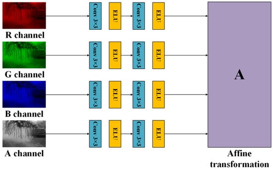
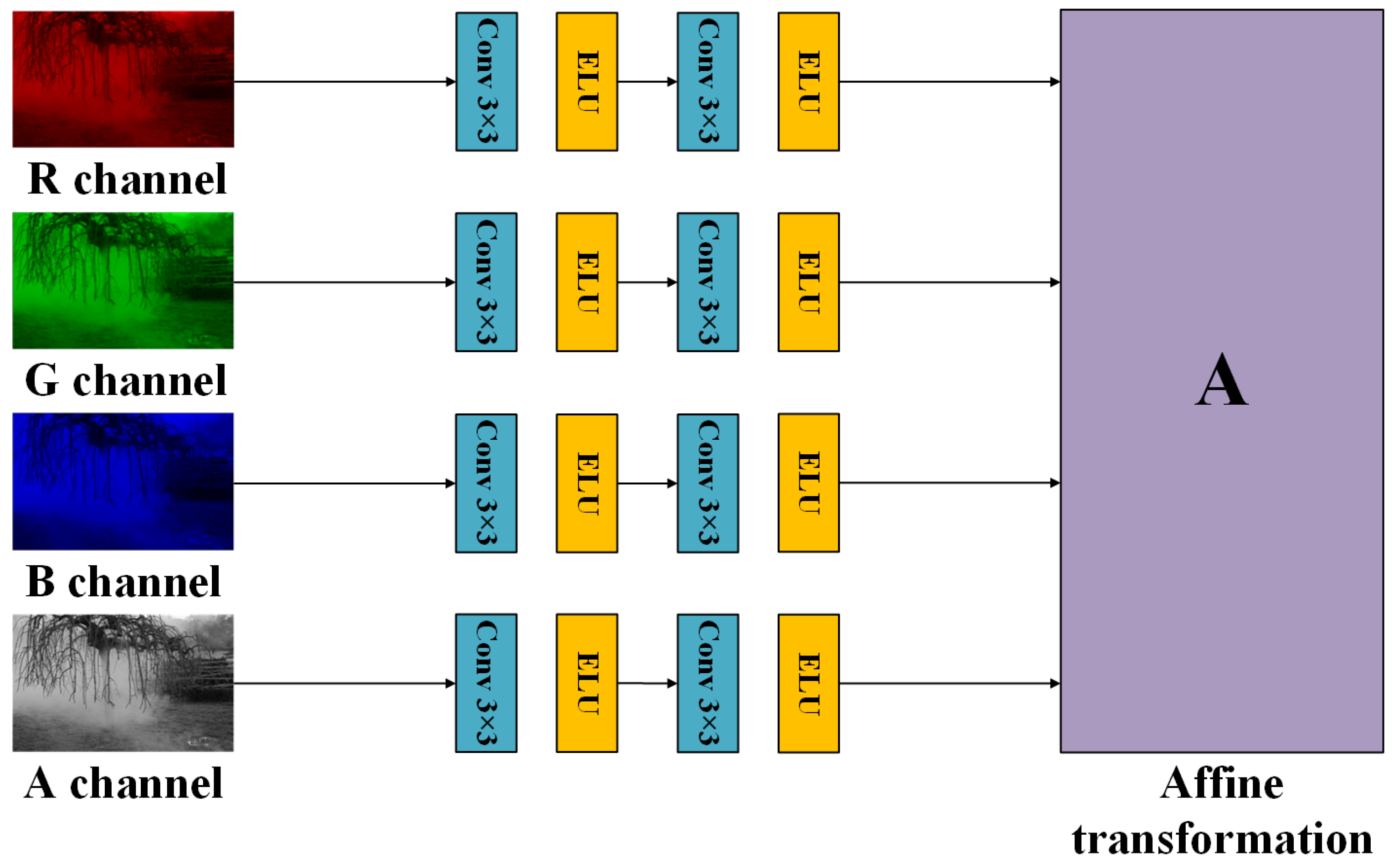
In the implementation process, for each color channel, we use two convolutional layers (3 × 3) and an ELU activation function to extract the guidance map separately, as shown in Figure 3.
Figure 3.
RGBA channel convolution.
After the generation of the guide maps for each channel, we can use this guide information to reconstruct the corresponding high-resolution features. This operation ensures that the information of each color channel is fully recovered, especially the edges and detailed parts of the image.
2.2.2. Feature Reconstruction
In this paper, we introduce a bilateral grid slicing operation after generating the guidance matrix to utilize the bilateral grid coefficients predicted by the low-resolution branches and transfer this information back to the full-resolution space of the original inputs to produce the image dehazing features.
First, we need to construct a guidance tensor using two coordinate guidance maps with the same dimensions as the input image, which are used to locate the feature values in the bilateral grid. Then, the trilinear interpolation method [23] is used to insert the bilateral grid data into the guidance tensor as a way of generating a high-dimensional feature tensor, which is represented by the following equation:
where the bilateral grid coefficients are and the guidance map is , and H is the generated high-dimensional feature tensor.
The formula for trilinear interpolation is as follows:
where represents the eight neighboring vertices in the bilateral grid and is the weight of the corresponding vertex.
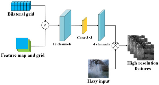
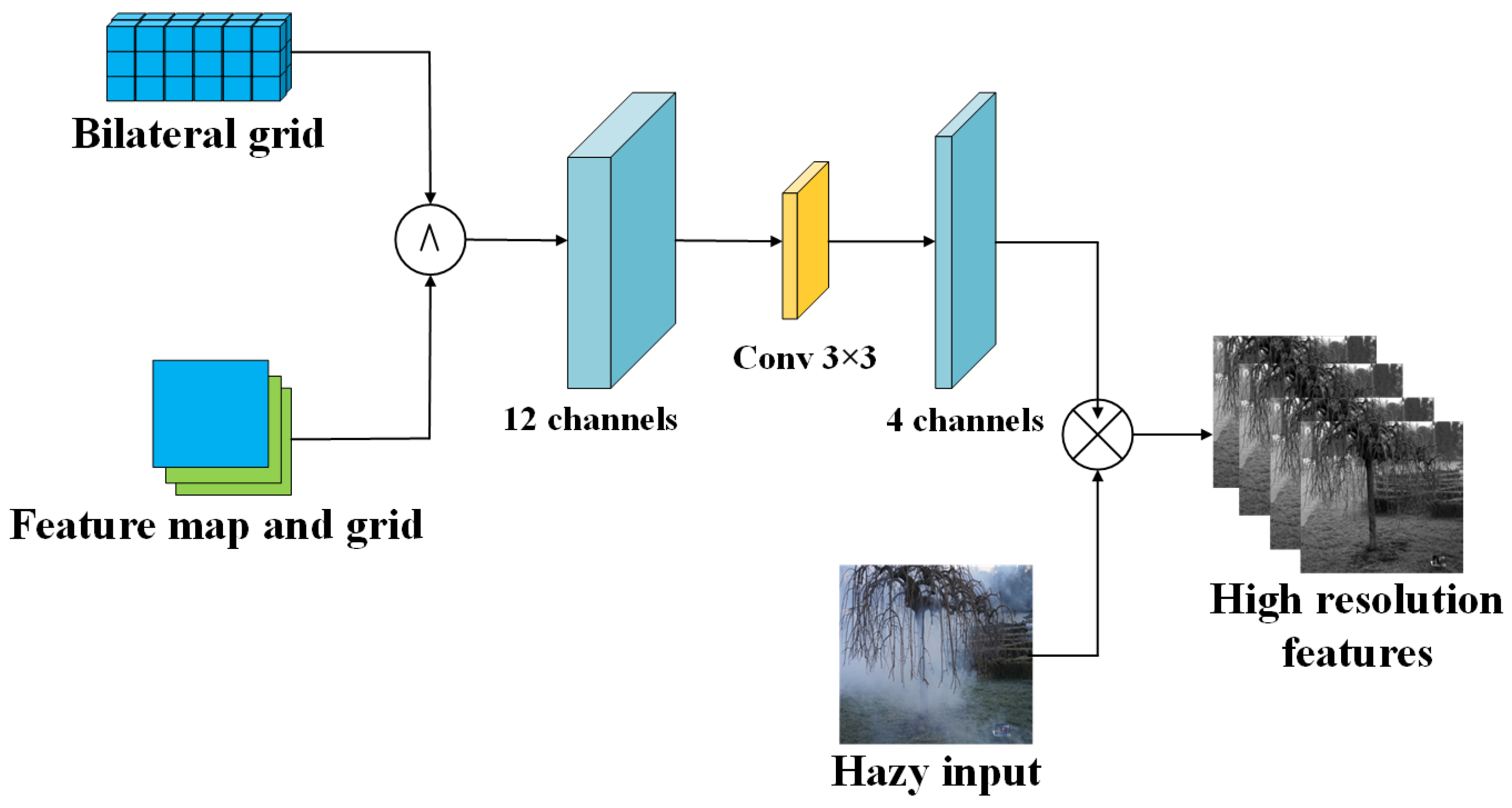
Figure 4 illustrates the reconstruction process from low-resolution features to full-resolution features. Specifically, it involves multi-channel input, where the RGB color channels and the atmospheric luminance channel (Channel A) are used to characterize the brightness changes caused by haze. The low-resolution features are used to learn the affine bilateral grid, and the grid coefficients are mapped to the full-resolution space through trilinear interpolation to capture the local structure and edge information of the image.
Figure 4.
High-resolution feature reconstruction based on bilateral grid and RGBA channels.
After generating a twelve-channel high-dimensional feature tensor, it is compressed to a four-channel tensor (corresponding to RGBA) through a 3 × 3 convolutional layer to retain the key information of each channel. The compressed feature tensor is then multiplied point-by-point with the original hazy image to enhance high-frequency details and color restoration, ultimately generating high-quality dehazed features.
2.3. CBAM Feature Fusion
After the feature reconstruction operation, we obtained high-quality de-fogged features. By connecting these high-quality de-fogged features with the original foggy image in a joining operation, we were able to obtain the de-fogged feature map. In the subsequent feature fusion, we first used the method of connecting multiple convolutional blocks to recover the final result, but this method has limited recovery in thick foggy regions. This may be due to the poor flexibility of feature fusion, where all feature channels and spatial locations are treated equally during fusion, and the model is unable to focus on the more important regions or features in the image, which leads to a weaker generalization ability of the model.
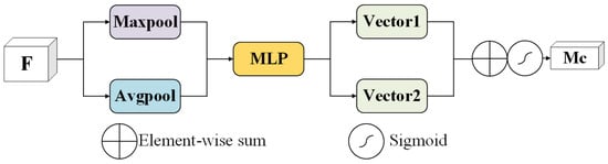
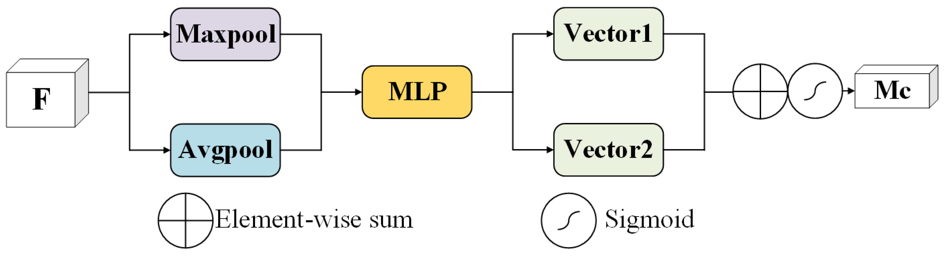
In order to solve this problem, this paper incorporates a CBAM module (convolutional block attention module) to improve it, and the main structure of the CBAM module includes a channel attention mechanism and a spatial attention mechanism [24,25]. Among them, the channel attention mechanism is used to generate the importance weight of each channel and enhance the response to important channels. Moreover, the spatial attention mechanism is used to generate the importance weight of each spatial location to highlight the important spatial regions in the image.
2.3.1. Channeling Attention Mechanisms
We perform maximum pooling and average pooling operations on the input feature maps (of size C × H × W) to compress the information of each channel in the spatial dimension, respectively, and finally compress it into an output of shape C × 1 × 1, where the shared network consists of two convolutions and a Relu activation function, as shown in Figure 5.
Figure 5.
Channel attention mechanism.
The channel attention mechanism captures global context information through global pooling and generates attention weights for each channel. First, we perform maximum pooling and average pooling for each channel of the feature graph to generate two global description vectors and , respectively, as follows:
The pooled descriptions and are then passed through the shared fully connected layer to generate the following channel attention weights:
where is the sigmoid activation function, is the Relu activation function, and are the MLP weights, and the original feature map is weighted channel-by-channel using the generated channel attention weights :
2.3.2. Spatial Attention Mechanisms
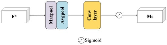
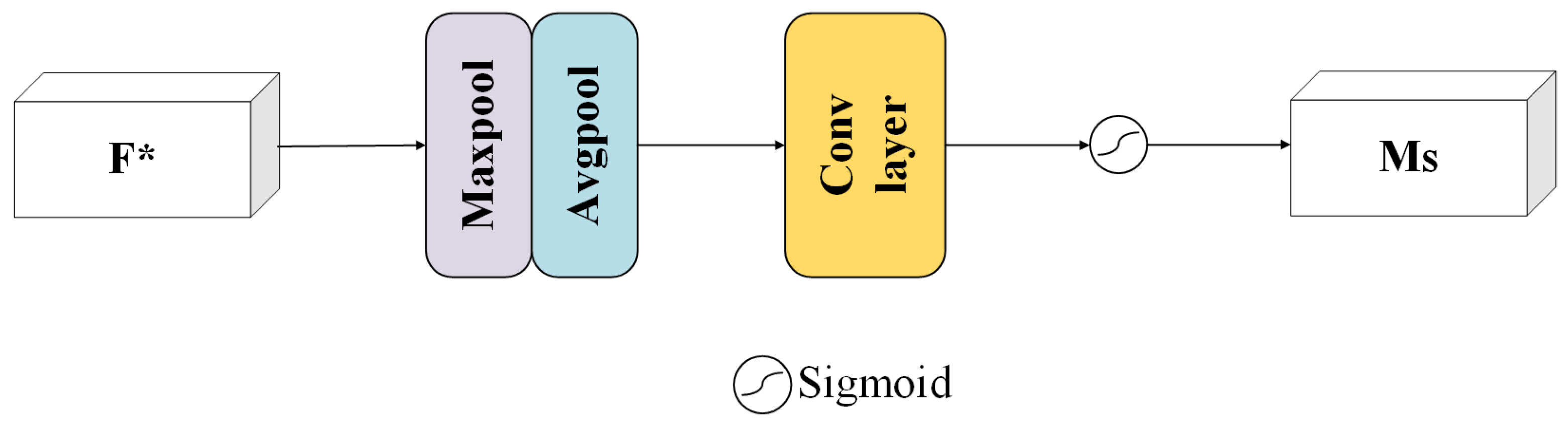
Similar to the channel attention mechanism, we perform maximum pooling and average pooling operations on the input feature maps along the channel axes to integrate the global channel information into a single channel feature map, which has the shape of 1 × H × W, as shown in Figure 6.
Figure 6.
Spatial attention mechanism.
The spatial attention mechanism generates a spatial weight map for enhancing important spatial regions in the image by aggregating the channel information of the feature map. First, in the channel dimension, we perform maximum pooling and average pooling operations on the channel-weighted feature map :
The results of maximum pooling and average pooling are then spliced and passed through a 7 × 7 convolutional layer to generate spatial attention weights :
where is the sigmoid activation function that applies the generated spatial attention weights to each spatial location of the channel-weighted feature map :
Finally, the fused feature map is combined with the input fogged image to generate the final de-fogged image:
At this point, we have obtained the final de-fogged image .
3. Experiments and Analysis of Results
3.1. Experimental Platform and Setup
The hardware platform for the experiments in this paper is a desktop computer with an Intel 13th i5-13600KF processor and NVIDIA GeForce RTX4070 12G GPU with Windows OS with CUDNNv8.3.2.
The data used for the experiments include both a public data and homemade datase. The public data are selected from the image dehazing benchmark dataset RESIDE, which contains synthetic blurred images of indoor and outdoor scenes from the depth dataset NYU Depth V2 and the stereo dataset Middlebury Stereo. The RESIDE Outdoor dataset is based on the stereo dataset Middlebury Stereo, which contains 8477 clear images and 296,695 blurred images generated from these clear images, with global atmospheric light values ranging from 0.8 to 1.0 and atmospheric scattering parameters ranging from 0.04 to 0.2 [22,26]. We use the ITS and OTS from these as a training dataset and evaluate the SOTS-Outdoor.
The Outdoor rail bolt dataset was chosen for the homebrew data, which contains 500 clear images of rail bolts and 500 fuzzy images of rail bolts.
3.2. Experimental Procedure
The network model in this paper is implemented using a PyTorch v2.1 framework and an Adam optimizer. An image with a resolution of 910 × 512 is applied to train the network, the initial learning rate is set to 0.001, the parameters are updated every 50 epochs of training, and 1000 epochs are trained.
3.2.1. Ablation Experiment
To demonstrate the effectiveness of each of the network modules presented in this paper, we set up four sets of experiments:
- No high-pass filtering module: no high-pass filtering module is introduced; instead, a general convolutional layer method is used for feature extraction operations, and other operations remain unchanged.
- No atmospheric luminance channel: no atmospheric luminance channel is introduced, i.e., the general color channels (R, G, B) are used to generate the guidance matrix, and other operations remain unchanged.
- No attention mechanism: Instead of introducing a CBAM module for feature fusion operation, a general convolutional layer method is used for feature fusion operation; other operations remain unchanged.
- Control experiment: the high-pass filter module, the atmospheric brightness channel, and the CBAM module are introduced into the model.
After conducting these four sets of experiments, we used the commonly used PSNR scores and SSIM scores to quantify the effects of the experiments in different situations, as shown in Table 1.
Table 1.
Validation of the effectiveness of each module.
According to Table 1, we can see that whether we use the public dataset or the homemade dataset, the experimental results are the best when all the modules are available, which suggests that all the modules can improve the de-fogging performance of the method in this paper; thus, the validity of the design can be proved. The de-fogging effects of Groups A, B, and C all significantly decrease the de-fogging effect relative to Group D, and the gap is the largest for Group C, which proves that the CBAM module in this paper improves the model performance the most, and the PSNR/SSIM improves from 31.97/0.9405 to 35.27/0.9869.
From the results, we found that the image dehazing effect of the public dataset has a significant improvement compared to the homemade dataset, which may be due to the fact that all of the homemade dataset comprises bolt images, which are too homogeneous in terms of color, texture, shape, and other features, leading to the lack of certain features in the public dataset. Thus, the image dehazing effect in the homemade dataset is poorer. We also tried to introduce some of the features from the public dataset into the homemade dataset in order to combine them into new data. However, in the end, we did not obtain any improvement.
3.2.2. CBAM Validity Testing
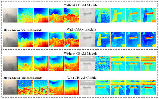
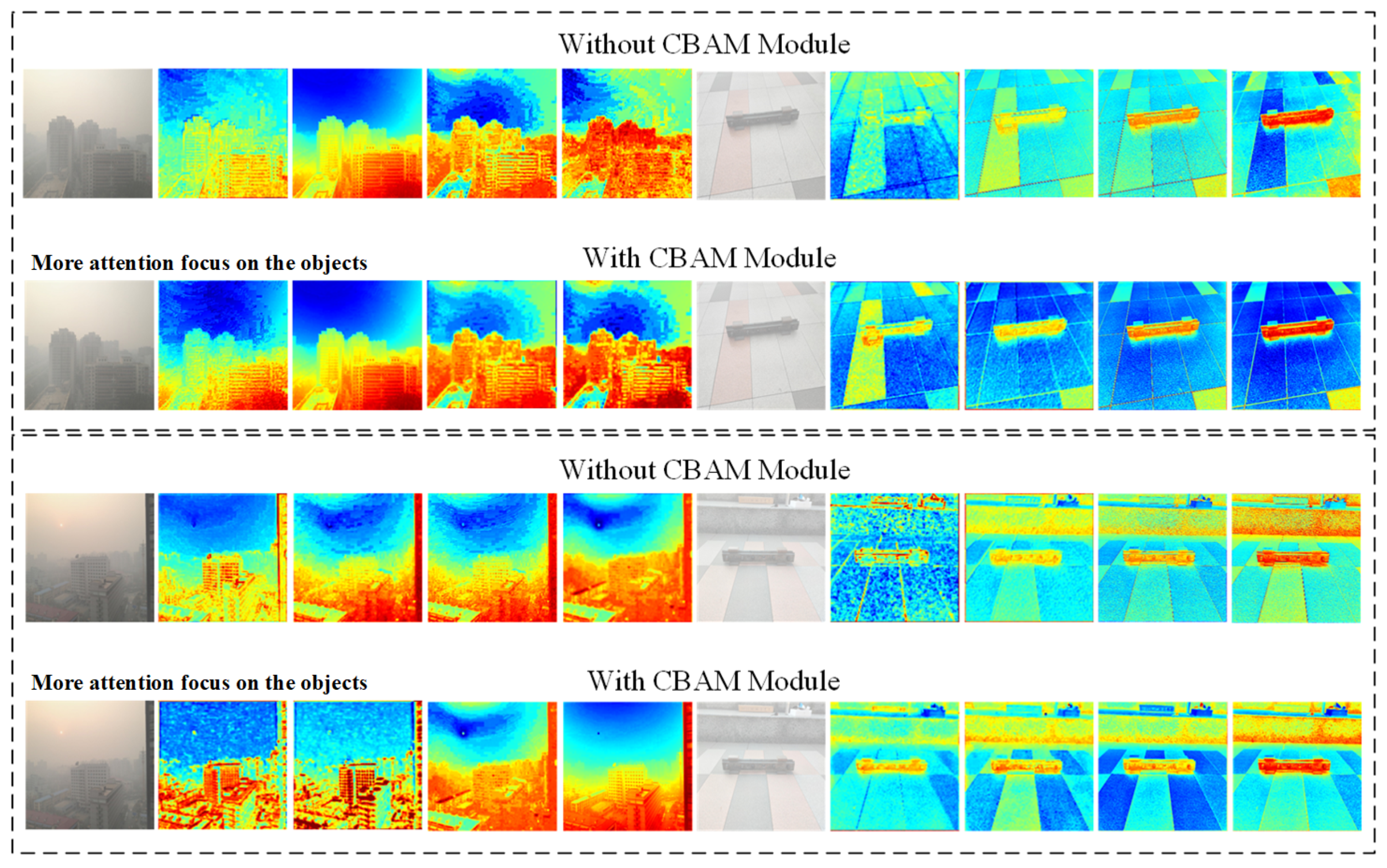
After the ablation experiments, we found that the CBAM module of this paper has the greatest impact on the final experimental results. For this reason, we used a heatmap approach to test the effectiveness of the CBAM module alone, as shown in Figure 7, where more red blocks of color are shown in the attentional region. On the other hand, in the inattentional region, more blue blocks of color are shown.
Figure 7.
CBAM heatmap visualization.
In Figure 7, the five columns on the left show the effect of the public dataset and the five columns on the right show the effect of the homemade dataset. With the same images, the top represents the effect without the CBAM module and the bottom represents the effect with the CBAM module. We can see that in both the public dataset and in the homemade dataset, the heatmap below changes faster than the one above and that the model’s attention is more likely to focus on the objects in the haze. This proves that the operation of adding the CBAM module is effective and necessary, and its can effectively improve the performance of the model in this paper.
3.2.3. Comparison Experiment
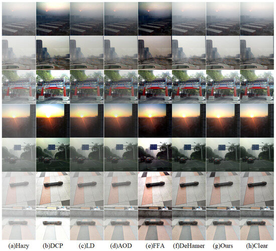
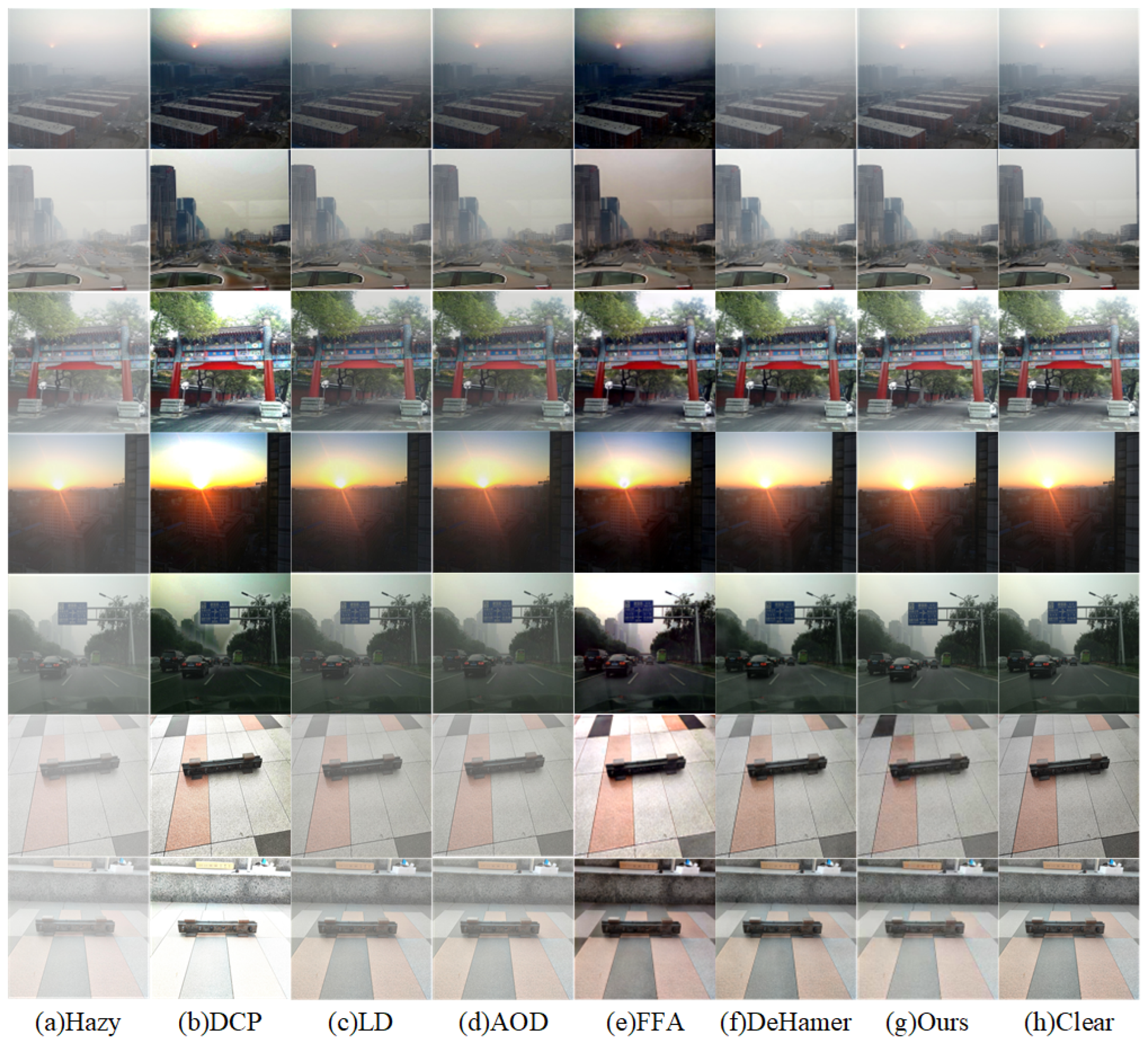
In order to verify the feasibility of the method in this paper, we compare the network model with several current image dehazing models ((b) DCP [7], (c) LDNet [15], (d) AODNet [16], (e) FFANet [17], and (f) DeHamer [18]) on the public dataset and homemade dataset, respectively, and the results of the comparisons are shown in Figure 8 and Table 2.
Figure 8.
Comparison of the effectiveness of multiple dehazing models.
Table 2.
Comparison of the effectiveness of different methods.
In Figure 8, the top five rows of images are from the public dataset, and the bottom two rows of images are from the homemade dataset, from which it can be seen that the outputs of DCP generally have some halos and artifacts. On the other hand, the outputs of LDNet and AODNet have obvious blurring effects in the homemade dataset, which cannot completely eliminate the haze. The outputs of FFA have some color distortions for both the ground and the sky, and there is excessive brightness. The output of DeHamer and the method in this paper is better and closer to the real clear image.
As can be seen from Table 2, the experimental results of the various methods on the public dataset are generally better than on the homemade dataset. The method of this paper performs best on the public dataset, with the highest PSNR and SSIM scores of all the methods, which are 35.27 and 0.9869, respectively. In the homemade dataset, the PSNR score of the method of this paper is also the highest (30.41), while the SSIM score (0.9511) is slightly inferior to DeHamer (0.9528) and 0.0017 lower than DeHamer. The results demonstrate the feasibility of this study. From the perspective of the algorithm’s real-time performance, the advantage of our model mainly lies in its lower FLOPs (floating-point operations per second), which means that the model has a smaller computational load, lower computational power requirements, and a higher inference efficiency. Although the number of parameters (Params) is not the smallest, the model achieves lower FLOPs while ensuring high performance. This reflects the efficiency of its algorithm design, which can achieve favorable results with fewer computations and strike a better balance in computational resource utilization.
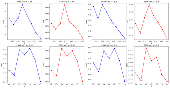
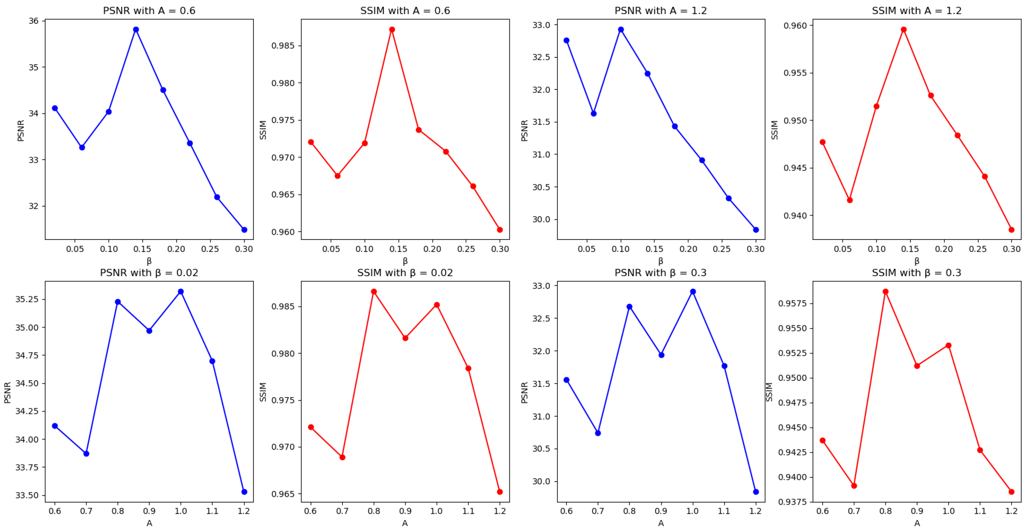
We further validate the algorithm’s performance under dynamic atmospheric changes. For the “dynamic atmospheric changes” scenario, we constructed an extended test set based on the RESIDE public dataset. We conducted performance comparisons under extreme parameter combinations and with single parameter variations. The comparison results are shown in Figure 9 and Table 3.
Figure 9.
Performance curve for single-parameter variations.
Table 3.
Comparison of dehazing methods under dynamic atmospheric parameter combinations.
As shown in Table 3, in the low-brightness light haze scenario (), the PSNR/SSIM of the proposed method is 1.67/0.0108 higher than that of the suboptimal algorithm, DeHamer, demonstrating an advantage in restoring low-contrast details. In the high-brightness heavy dense haze scenario (), the proposed method achieves PSNR/SSIM values of 29.84/0.9385, representing an improvement of 2.72/0.0358 over DeHamer, which verifies its robustness under strong scattering interference.
In Figure 9, the atmospheric light value (A) was expanded from the original range [0.8, 1.0] to [0.6, 1.2], generating seven values at intervals of 0.1. The scattering coefficient was expanded from [0.04, 0.2] to [0.02, 0.3], generating eight values at intervals of 0.04. A total of 56 sets (7 × 8) of hazy images with different parameter combinations were synthesized using the atmospheric scattering model , with each combination containing 100 test images (5600 images in total). When fixing and increasing (from light to dense haze), PSNR first increases and then decreases, peaking at , indicating the algorithm optimally handles moderate haze concentrations.
With fixed at 0.3 and A increasing from low to high brightness: The PSNR/SSIM exhibits a fluctuating downward trend as A increases, reaching the highest value at and decreasing to 29.84/0.9385 at , reflecting the impact of extreme high-brightness conditions on atmospheric light estimation.
The method proposed in this paper provides a new technical path for cross-domain image dehazing in railway scenarios through multi-channel feature decoupling and the CBAM attention mechanism. It aligns with optimized algorithms such as “feature hierarchy to mitigate domain differences” and “prototype alignment” in [27], and clarifies the improvement directions for class-imbalanced data and explicit domain alignment. We are deeply aware of the impact of the limitations of self-built datasets on the model’s generalization ability. In the future, we will further expand the diversity of the dataset and incorporate strategies such as “prototype alignment” from [27] to optimize cross-domain feature learning, so as to promote the reliable application of the algorithm in actual railway detection scenarios.
As a phased achievement in railway image dehazing, the current research has verified the effectiveness of the algorithm in conventional scenarios.
4. Concluding Remarks
In this paper, an improved adaptive high-pass filter module is added to the existing convolutional layer feature extraction method, in which a Laplace filter is added, which directly improves the efficiency of feature extraction; in addition, in the feature reconstruction, an atmospheric luminance channel is added on the basis of the three RGB color channels, which improves the accuracy of the color features on the basis of the original; moreover, combined with the CBAM attention module, the features are fused to obtain the final de-fogged image. Through the comparison experiments in the public dataset RESIDE and the homemade dataset, it is proved that the method of this paper is better than most of the other methods. Thus, it demonstrates a certain degree of feasibility and research value.
However, current methods have limitations: in terms of global representation, they rely on the local feature extraction capability of CNNs while lacking explicit modeling of the global topological structure of images. In terms of data generalization capability, due to the dependence of deep learning on large-scale data, models are prone to overfitting on small-sample datasets in specific scenarios, such as railway bolts. The SSIM index of the self-constructed dataset is slightly lower than that of the DeHamer method, reflecting an insufficient robust representation of structural priors. Additionally, although geometric features are implicitly processed through RGBA channels and attention mechanisms, the lack of explicit topological connectivity constraints further affects detection accuracy.
To address the above issues, we plan to focus on the optimization direction of integrating persistent homology theory [28] in future research. Specifically, we intend to introduce the persistent homology theory into the feature extraction module to capture global topological structures at multiple scales. By analyzing the structural stability of clear images using persistent homology, we will establish a topological prior for the transmission map to improve the accuracy of transmission map estimation. We will design a lightweight fusion framework with a hierarchical network structure: shallow networks will retain CNNs to extract local texture features, while deep networks will embed persistent homology processing for global structures. Meanwhile, persistent homology features will be mapped into low-dimensional vectors to serve as attention weights, focusing on key regions to balance the model’s efficiency and performance. Additionally, we will extract general topological features from railway scenarios for few-shot and cross-domain migration, enhancing the model’s generalization ability to new data.
The self-constructed dataset lacks diverse railway scenarios, which restricts the model’s application in real environments. In subsequent research, we plan to build a multi-scenario dataset to enhance the scene richness of the data, integrate cross-modal data by combining multi-modal sensor data such as infrared and LiDAR, and construct a railway scenario dataset that includes depth information.
In addition, there is still much room for improvement and optimization of our proposed method. Moreover, the algorithm can be explored in more depth to meet the more stringent requirements for image quality in the future. The homemade dataset can also be improved to make it more applicable to the research and detection of multiple methods. We can also improve our self-developed dataset to make it more suitable for the research and detection of multiple methods.
Author Contributions
Conceptualization, H.X., Z.C., S.L. and S.H.; methodology, H.X. and S.H.; software, H.X. and K.X.; writing—original draft preparation, Z.C. and S.C.; writing—review and editing, S.H., S.L. and J.T.; visualization, S.H., Z.C. and H.X.; supervision, Z.C. and K.X.; investigation, S.C.; funding acquisition, W.Z.; project administration, K.X. and W.Z. All authors have read and agreed to the published version of this manuscript.
Funding
This work was supported by the National Natural Science Foundation of China (Nos. 62373372 and 62272485), the Innovative Entrepreneurship Undergraduate Training Programme [Grant No. Yz2024410] at Yangtze University, and the National Innovative Entrepreneurship Undergraduate Training Programme (Grant No. 202410489004).
Data Availability Statement
The data used in this study are unavailable due to privacy restrictions.
Acknowledgments
We gratefully acknowledge all the members who participated in this work.
Conflicts of Interest
The authors declare no conflicts of interest.
References
- Jiang, H.; Ma, Q.; Cao, S.; Wang, Z. Researchand Application on Railway Vehicle Running Safety Monitor System (5T). J. Highw. Transp. Res. Dev. 2009, 26, 1–6. [Google Scholar]
- Wang, Y.; Cai, X.; Tang, X.; Pan, S.; Wang, Y.; Yan, H.; Ren, Y.; Hou, Y. HSRA-Net: Intelligent Detection Network of Anomaly Monitoring Data in High-Speed Railway. IEEE Trans. Intell. Transp. Syst. 2024, 25, 20793–20803. [Google Scholar] [CrossRef] [Scilit]
- Asha, C.S.; Siddiq, A.B.; Akthar, R.; Rajan, M.R.; Suresh, S. ODD-Net: A hybrid deep learning architecture for image dehazing. Sci. Rep. 2024, 14, 30619. [Google Scholar] [CrossRef] [Scilit] [PubMed]
- Vishnoi, R.; Goswami, P.K. A Comprehensive Review on Deep Learning based Image Dehazing Techniques. In Proceedings of the International Conference on System Modeling and Advancement in Research Trends (SMART), Moradabad, India, 16–17 December 2022; pp. 1392–1397. [Google Scholar]
- Lv, X.; Chen, W.; Shen, I. Real-Time Dehazing for Image and Video. In Proceedings of the Pacific Conference on Computer Graphics and Applications, Hangzhou, China, 25–27 September 2010; pp. 62–69. [Google Scholar]
- Jin, Y.; Chen, J.; Tian, F.; Hu, K. LFD-Net: Lightweight Feature-Interaction Dehazing Network for Real-Time Remote Sensing Tasks. IEEE J. Sel. Top. Appl. Earth Obs. Remote Sens. 2023, 16, 9139–9153. [Google Scholar] [CrossRef] [Scilit]
- He, K.; Sun, J.; Tang, X. Single image haze removal using dark channel prior. IEEE Trans. Pattern Anal. Mach. Intell. 2010, 33, 2341–2353. [Google Scholar] [PubMed]
- Wu, R.; Duan, Z.; Guo, C.; Chai, Z.; Li, C. Ridcp: Revitalizing real image dehazing via high-quality codebook priors. In Proceedings of the IEEE/CVF Conference on Computer Vision and Pattern Recognition, Vancouver, BC, Canada, 17–23 June 2023; pp. 22282–22291. [Google Scholar]
- Galteri, L.; Seidenari, L.; Bertini, M.; Del Bimbo, A. Deep generative adversarial compression artifact removal. In Proceedings of the IEEE International Conference on Computer Vision, Venice, Italy, 22–29 October 2017; pp. 4826–4835. [Google Scholar]
- Cai, B.; Xu, X.; Jia, K.; Qing, C.; Tao, D. Dehazenet: An end-to-end system for single image haze removal. IEEE Trans. Image Process. 2016, 25, 5187–5198. [Google Scholar] [CrossRef] [Scilit] [PubMed]
- Li, L.; Dong, Y.; Ren, W.; Pan, J.; Gao, C.; Sang, N.; Yang, M. Semi-Supervised Image Dehazing. IEEE Trans. Image Process. 2020, 29, 2766–2779. [Google Scholar] [CrossRef] [Scilit] [PubMed]
- Ren, W.; Pan, J.; Zhang, H.; Cao, X.; Yang, M.-H. Single image dehazing via multi-scale convolutional neural networks with holistic edges. Int. J. Comput. Vis. 2017, 128, 240–259. [Google Scholar] [CrossRef] [Scilit]
- Song, Y.; Li, J.; Wang, X.; Chen, X. Single image dehazing using ranking convolutional neural network. IEEE Trans. Multimed. 2009, 20, 1548–1560. [Google Scholar] [CrossRef] [Scilit]
- Guo, Q.; Huang, Y. Image dehazing algorithm based on DehazeNet and edge detection mean-guided filtering. Transducer Microsyst. Technol. 2020, 39, 150–153. [Google Scholar]
- Ullah, H.; Muhammad, K.; Irfan, M.; Anwar, S.; Sajjad, M.; Imran, A.S.; de Albuquerque, V.H.C. Light-DehazeNet: A novel lightweight CNN architecture for single image dehazing. IEEE Trans. Image Process. 2021, 30, 8968–8982. [Google Scholar] [CrossRef] [Scilit] [PubMed]
- Li, B.; Peng, X.; Wang, Z.; Xu, J.; Feng, D. An all-in-one network for dehazing and beyond. arXiv 2017, arXiv:1707.06543. [Google Scholar]
- Qin, X.; Wang, Z.; Bai, Y.; Xie, X.; Jia, H. FFA-Net: Feature fusion attention network for single image dehazing. In Proceedings of the AAAI Conference on Artificial Intelligence, New York, NY, USA, 7–12 February 2020; Volume 34, pp. 11908–11915. [Google Scholar]
- Guo, C.; Yan, Q.; Anwar, S.; Cong, R.; Ren, W.; Li, C. Image dehazing transformer with transmission-aware 3d position embedding. In Proceedings of the IEEE/CVF Conference on Computer Vision and Pattern Recognition, New Orleans, LA, USA, 18–24 June 2022; pp. 5812–5820. [Google Scholar]
- Lu, Z.; Li, J.; Liu, H.; Huang, C.; Zhang, L.; Zeng, T. Transformer for single image super-resolution. In Proceedings of the IEEE/CVF Conference on Computer Vision and Pattern Recognition, New Orleans, LA, USA, 18–24 June 2022; pp. 457–466. [Google Scholar]
- Gao, G.; Cao, J.; Bao, C.; Hao, Q.; Ma, A.; Li, G. A novel transformer-based attention network for image dehazing. Sensors 2022, 22, 3428. [Google Scholar] [CrossRef] [Scilit] [PubMed]
- Sameh Arif, A.; Mansor, S.; Logeswaran, R. Combined bilateral and anisotropic-diffusion filters for medical image de-noising. In Proceedings of the 2011 IEEE Student Conference on Research and Development, Cyberjaya, Malaysia, 19–20 December 2011; pp. 420–424. [Google Scholar] [CrossRef] [Scilit]
- Zheng, Z.; Ren, W.; Cao, X.; Hu, X.; Wang, T.; Song, F.; Jia, X. Ultra-high-definition image dehazing via multi-guided bilateral learning. In Proceedings of the IEEE/CVF Conference on Computer Vision and Pattern Recognition (CVPR), Nashville, TN, USA, 20–25 June 2021; pp. 16180–16189. [Google Scholar]
- Chen, J.; Paris, S.; Durand, F. Real-time edge-aware image processing with the bilateral grid. ACM Trans. Graph. (TOG) 2007, 26, 103-es. [Google Scholar] [CrossRef]
- Woo, S.; Park, J.; Lee, J.Y.; Kweon, I.S. CBAM: Convolutional block attention module. In Proceedings of the European Conference on Computer Vision (ECCV), Munich, Germany, 8–14 September 2018; pp. 3–19. [Google Scholar]
- Brauwers, G.; Frasincar, F. A general survey on attention mechanisms in deep learning. IEEE Trans. Knowl. Data Eng. 2021, 35, 3279–3298. [Google Scholar] [CrossRef] [Scilit]
- Li, B.; Ren, W.; Fu, D.; Tao, D.; Feng, D.; Zeng, W.; Wang, Z. Benchmarking single-image dehazing and beyond. IEEE Trans. Image Process. 2018, 28, 492–505. [Google Scholar] [CrossRef] [Scilit] [PubMed]
- Fang, X.; Easwaran, A.; Genest, B.; Suganthan, P.N. Your data is not perfect: Towards cross-domain out-of-distribution detection in class-imbalanced data. Expert Syst. Appl. 2025, 267, 126031. [Google Scholar] [CrossRef] [Scilit]
- Wang, C.; Cao, R.; Wang, R. Learning discriminative topological structure information representation for 2D shape and social network classification via persistent homology. Knowl.-Based Syst. 2025, 311, 113125. [Google Scholar] [CrossRef] [Scilit]

Disclaimer/Publisher’s Note: The statements, opinions and data contained in all publications are solely those of the individual author(s) and contributor(s) and not of MDPI and/or the editor(s). MDPI and/or the editor(s) disclaim responsibility for any injury to people or property resulting from any ideas, methods, instructions or products referred to in the content. |
© 2025 by the authors. Licensee MDPI, Basel, Switzerland. This article is an open access article distributed under the terms and conditions of the Creative Commons Attribution (CC BY) license (https://creativecommons.org/licenses/by/4.0/).