


Abstract
Early-stage planning of floating marine renewable energy infrastructures can benefit from identifying areas with favorable hydrodynamic conditions. Hydrodynamic stability assessment can support the planning of floating photovoltaic systems, offshore wind turbines, and renewable hydrogen production facilities. This study presents a transferable, data-driven multivariate framework that quantifies hydrodynamic variability to identify areas of higher relative hydrodynamic stability for marine renewable energy site selection. It integrates sea surface potential temperature, salinity, water velocity, wave characteristics, and bathymetry; quantifies temporal variability using waveform length; and combines the resulting variable layers through a hybrid stability index and parametric weighting procedure. Applied to Spanish marine subdivisions shallower than 1000 m using Marine Copernicus data, the results show that wave-related variability is the dominant contributor, while the Levantine–Balearic subdivision exhibits the largest relative extent of stable zones and the highest overall relative stability under global normalization. The resulting relative stability index provides a transferable hydrodynamic pre-screening layer that can be integrated into Geographic Information System (GIS)-based marine spatial planning before technology-specific renewable-resource and other planning assessments.
Keywords:
decision-making; floating; hydrodynamics; planning; renewables; siting; stability; variability 1. Introduction
Oceans and seas are dynamic natural systems that interact complexly with the atmosphere and Earth’s surface, forming part of a coupled global system in which matter and energy are continuously exchanged [1]. Spatial variations in ocean temperature and salinity, together with Earth’s rotation, gravitational forces, and atmospheric processes, drive water movements both at the surface and at depth, giving rise to a three-dimensional ocean circulation that operates across multiple spatial and temporal scales [2,3,4]. This circulation not only plays a fundamental role in the redistribution of heat, salt, and other physical and biogeochemical properties, but also contributes decisively to climate regulation and the Earth’s energy balance [2,3], as oceans and seas act as the primary heat reservoirs and modulate the planet’s thermal response [5].
The interaction between ocean circulation and seabed topography actively shapes submarine relief and coastal zones through erosion and sedimentation processes influenced by ocean dynamics, atmospheric forcing, and continental inputs [6,7,8]. The vertical and horizontal motions associated with this circulation regulate nutrient availability in the surface layer, thereby controlling biological productivity and the distribution of marine ecosystems [9,10]. Additionally, ocean dynamics make the marine environment a natural and virtually inexhaustible source of renewable energy [11,12,13,14]. The higher density of seawater compared to air, together with the greater predictability of marine energy resources relative to other renewable energy sources [15], gives the marine environment a high potential for electricity generation. This potential has attracted increasing interest in recent years [16,17,18,19,20,21,22].
However, despite the significant growth potential in the design and deployment of ocean-based power generation technologies [22], their large-scale development remains constrained by substantial technical and operational challenges associated with continuous operations in the marine environment [23,24]. These challenges are particularly pronounced in systems whose installation, operation, or maintenance is conducted underwater, at great depths, and far from the coast, where extreme environmental conditions increase technical complexity, operational risks, and associated costs.
As reported in previous studies [25,26], Spain has strong industrial and technological potential in the field of renewable energy, ranking as the second country in Europe and the fifth worldwide in installed wind power capacity. Furthermore, it benefits from a well-established shipbuilding industry, a consolidated maritime–port sector, extensive research and civil engineering capabilities, and an industrial ecosystem for manufacturing materials and equipment that supports the development of marine renewable energy and facilitates its future deployment in deep waters.
Floating marine renewable energy structures deployed in shallow to moderate-depth waters represent a more technologically viable alternative in Spain, as they simplify installation, operation, and maintenance requirements, as well as grid connection to the mainland. Within this framework, examples include offshore wind turbines and floating solar energy systems for direct electricity supply and/or green hydrogen production [27,28]. Identifying favorable hydrodynamic conditions for these technologies may support more favorable operating conditions by limiting wave- and current-induced platform motions. For floating photovoltaic and photovoltaic–hydrogen systems, platform motion and wave-induced spatial disturbances can modify the orientation of the active surface relative to incident solar radiation and affect the operating conditions of the associated energy-conversion and hydrogen-production systems [27,29,30]. Similarly, in floating wind turbines, wave-induced platform dynamics can modify rotor motion, orientation, and the apparent wind experienced by the turbine, thereby affecting power production [31]. Recent high-fidelity FOWT studies further demonstrate that the accurate representation of environmental loads, wave–current effects, and platform dynamics is essential for predicting motion and mooring responses under demanding operating conditions [32]. These hydrodynamic effects should nevertheless be considered separately from renewable resource availability, which must be assessed using technology-specific information such as solar irradiance or wind conditions.
These solutions reduce the technical complexity of offshore operations and contribute to lowering the levelized cost of energy (LCOE), thereby enhancing the economic viability of marine power generation systems [23].
These types of marine structures are particularly relevant in Spain due to its geographical and geodynamic setting [33]. The interaction between tectonic, hydrodynamic, and sedimentary processes has shaped the configuration of its continental margins [33,34,35]. As a result, the submerged continental shelf—characterized by shallow to moderate depths—often exhibits a limited width of only a few kilometers, followed by a steep slope toward the continental margin and abyssal zones [33,34].
The development and installation of marine platforms in the country depend on the following factors [25,36]: (i) aligning these installations with national energy and climate strategies and with the applicable regulatory framework of the host country, which establish maritime spatial planning criteria and define suitable or restricted areas for the development of marine renewable energy; and (ii) accounting for the dynamic and stability conditions of the ocean at the installation site. This approach facilitates the site selection process and supports the selection and design of suitable platforms as part of a broader marine energy planning framework.
Marine spatial planning and offshore renewable energy site selection commonly rely on Geographic Information Systems (GISs), which allow spatial data to be analyzed and represented as thematic map layers [37]. Recent studies have combined GIS-based and multi-criteria frameworks to integrate different technical, environmental, economic, resource-related, logistical, infrastructural, and met-ocean criteria [38,39,40]. These constraints commonly include, among others, bathymetry, protected areas, renewable resources, wave climate, and operational thresholds [37,39,41]. These approaches are frequently coupled with Multi-Criteria Decision-Making (MCDM), Multiple Attribute Decision Analysis (MADA), or Analytic Hierarchy Process (AHP) methods to rank candidate sites [42,43,44]. Recent applications include offshore wind and floating wind site selection [41,42,44], offshore solar and floating solar-related applications [27,28,45], hybrid offshore wind–solar frameworks [37,40], floating energy islands [39], and Spanish floating offshore wind case studies [46].
Recent studies on marine-current energy converters further show that hydrodynamic design and operating conditions can substantially influence device performance, highlighting the importance of characterizing the surrounding marine environment as part of the broader planning and design process [47]. However, the outcome of GIS–MCDM, MADA, or AHP frameworks may depend on the selected criteria and relative weights [43,45,48]. This dependence is particularly relevant when expert judgement or predefined weighting scenarios are used to combine heterogeneous technical, economic, environmental, logistical, or met-ocean criteria [42,43,46].
The present study complements these approaches by introducing a data-driven hydrodynamic pre-screening layer for marine renewable energy site selection and planning. Rather than ranking candidate sites mainly according to resource availability, economic feasibility, infrastructure proximity, or regulatory constraints, the proposed framework focuses on the dynamic stability of the marine environment. It integrates a set of marine variables—including sea surface potential temperature, salinity, water velocity components, wave characteristics, and bathymetry—quantifies their temporal variability using the waveform-length metric, and combines them through a hybrid stability index to identify spatial clusters of comparatively stable marine zones that can support the early-stage planning of floating renewable energy infrastructures, including floating wind, floating solar, and hybrid offshore energy platforms. The resulting hydrodynamic layer is intended as a pre-screening criterion and should subsequently be combined with technology-specific resource information, such as wind conditions for wind energy or solar irradiance for photovoltaic applications, together with other technical, environmental, and economic criteria.
The methodology is general and transferable to nearshore and offshore areas worldwide and across different temporal ranges, provided that georeferenced time series of the selected marine variables are available. Its application is therefore not restricted to Spanish waters or to the temporal range considered in this case study and can be adapted to other marine regions and analysis periods by using equivalent oceanographic datasets and, when required, by adding, removing, or replacing input variables according to regional conditions and specific analysis requirements. Importantly, the relative contribution of the selected variables is explored automatically through a parametric weighting procedure, avoiding dependence on a single predefined weighting scenario. The resulting spatial stability index is interpretable and can be incorporated as an additional GIS layer in marine spatial planning and decision-support workflows. Accordingly, the main contribution of the framework lies in providing a transferable and spatially resolved procedure for integrating multiple physical drivers of surface hydrodynamic variability and identifying areas of higher relative stability at a finer spatial scale than broad regional classifications.
Spain is used here as a case study because of its diverse Atlantic and Mediterranean coastal domains and island systems, which provide contrasting marine environments in which to evaluate the proposed framework, as well as its strong naval, shipbuilding, port, and offshore engineering capabilities, as reflected in recent maritime spatial planning analyses for offshore wind energy in Spanish waters [25,26,49].
2. Materials and Methods
The first step in the proposed methodology is to define the geographical areas on which the study focuses. In this case, Spanish marine territory is divided into five subdivisions [50]: North Atlantic, South Atlantic, Strait and Alboran, Levantine–Balearic, and Canary (Figure 1).
Figure 1.
Geographical zones of Spain: Marine subdivisions. Base map: Cartopy/Natural Earth.
All ocean variable data used as input in this study were provided by and downloaded from Marine Copernicus [51]. Marine Copernicus is the European ocean observation and forecasting service and is part of the European Union’s Copernicus Programme.
As shown in Table 1, this study uses two Marine Copernicus products: (i) P1: Atlantic–Iberian Biscay Irish–Ocean Physics Analysis and Forecast [52]; and (ii) P2: Atlantic–Iberian Biscay Irish–Ocean Wave Analysis and Forecast [53]. These products provide high-resolution analyses and forecasts of the ocean’s physical state in the Iberia–Biscay–Ireland (IBI) region, within the geographical bounds of 19° W to 5° E and 26° N to 56° N, with a spatial grid resolution of 1/36° (≈2–3 km).
Table 1.
Marine Copernicus products used in this study.
Table 2 and Table 3 present the set of multidimensional ocean variables considered in this study, included within the previously described products, P1 and P2. Here, longitude is denoted by , latitude by , time by t, and the measurement depth of the variable by d.
Table 2.
P1 product: Variable selection and definition.
Table 3.
P2 product: Variable selection and definition.
The variables were processed at the native temporal resolution of their respective Copernicus products, namely daily for the P1 variables and hourly for the P2 wave variables. No temporal interpolation or resampling to a common temporal resolution was performed. Importantly, for each individual variable, the temporal resolution is identical at all geographical locations considered in the analysis. Therefore, the same temporal sampling and the same mathematical transformation are applied to every time series belonging to a given variable, preserving the relative geospatial pattern of temporal variability within that data layer.
For clarity, Figure 2 presents the methodological diagram of the study, in which four phases are defined: (i) Ocean Variables, including all steps required to access and retrieve the ocean variables used as inputs for the analysis; (ii) Waveform Length, used to extract the temporal variability of the ocean variables as a key feature; (iii) Normalization, applied to reduce the influence of outliers and ensure that all variables lie within the interval ; (iv) Identification and Clustering, used to determine geographical locations that meet the defined stability criteria, and to group individual stable locations into stable zones and exclude the remaining areas.
Figure 2.
Methodological diagram of the present study for the calculation of marine stability zones.
2.1. Mathematical Model: Multivariable Hydrodynamic Analysis—Ocean Variables, Waveform Length, Normalization, Identification, and Clustering
Oceans and seas are dynamic natural systems [1] that operate across multiple spatial and temporal scales [2,3,4]. The ocean variables that describe them are coupled not only physically but also across temporal and spatial dimensions, as the state at a given ocean location influences, to varying degrees, both its future states and those of adjacent regions. This interaction enables the existence of geographical areas with similar variability patterns, which can be identified through the individual and collective analysis of data associated with these variables.
In this study, each ocean variable is generically represented as , where x denotes the variable identifier, its geographical position, and t its temporal dimension. For each location , x is described by a sequential data series—composed of N values—that captures its temporal evolution. The value of N is determined by the time range under study and the variable’s sampling period (Ts).
2.1.1. PHASE I: Ocean Variables
The ocean variables shown in Table 2 and Table 3 are downloaded from the Marine Copernicus service in NetCDF4 format and subsequently imported into Python (version 3.12.3) for processing using the mathematical model presented below. The downloaded data are then masked, first according to the defined geographical boundaries and subsequently based on their associated depth (deptho).
2.1.2. PHASE II: Waveform Length
The instability of is defined as a key feature and, following previous studies [54], is computed using the mathematical model known as waveform length (:
The key feature represents the mean absolute change between consecutive observations of variable x over the analyzed temporal range. Because Equation (1) normalizes the accumulated absolute changes by the number of consecutive intervals (N − 1), a larger number of observations does not, by itself, produce a larger value. Higher values indicate greater temporal variability or dynamic activity, whereas lower values indicate comparatively more stable temporal behavior. For each variable, is calculated using the same temporal resolution and mathematical transformation at all geographical locations, allowing the relative spatial distribution of temporal variability to be characterized within that variable. Consequently, the framework does not directly compare raw waveform-length magnitudes between variables sampled at different temporal resolutions. By incorporating the absolute changes between consecutive observations, waveform length preserves the sequential evolution of the signal and provides a direct descriptor of its temporal activity over the analyzed period. Its formulation is computationally simple and maintains sensitivity to changes in amplitude, noise, trend, and temporal variability [54,55]. Furthermore, it is insensitive to the mean value of the signal.
is defined as the two-dimensional matrix that groups the set of points , computed for a given variable x, and is used to store, in an ordered manner, the logical relationships among the different values within the same marine subdivision [50]. While —applied to the ocean variables thetao, so, uo, vo and wo—is computed directly from Equation (1), its calculation for characterizing instability induced by surface and deep-water waves requires special consideration due to the interdependence of multiple ocean variables. Accordingly, to compute wave-induced instability at the surface, is redefined as in Equation (2). The variable represents deep-water wave power as a proportional relationship between wave amplitude (vhm0) and wave period (vtm10).
Furthermore, the proposed mathematical model also accounts for wave direction (vmdr) when calculating wave-induced instability. Because vmdr is an angular variable, its temporal variability at each geographical location is quantified using circular variance in [0, 1] [56,57]. Each angular observation can be represented as a unit vector whose Cartesian components are given by its cosine and sine values. The mean resultant vector is obtained by averaging these components over the N observations, and its magnitude, denoted by , represents the degree of directional concentration of the data. When all directions are similar, the unit vectors point in nearly the same direction and approaches 1, indicating high directional consistency. Conversely, when the directions are widely dispersed, the vectors tend to cancel each other and approaches 0, indicating low directional consistency. Circular variance is therefore defined as , so that V approaches 0 for highly concentrated directions and approaches 1 for highly dispersed directions. Accordingly, the normalization factor used to calculate the mean sine and cosine components in Equation (3) is 1/N, consistently with the standard definition of circular variance.
where represents locations with high directional stability of waves, and indicates high instability.
Based on this, and following Equations (2) and (3), is defined as:
where the factor applies a penalty to the initially computed , in proportion to the circular variability at that location .
2.1.3. PHASE III: Normalization
represents the matrix robustly normalized according to Equations (5) and (6). This normalization is performed independently for each variable layer before multivariable integration. Therefore, the model combines the relative spatial variability represented by the normalized layers rather than directly accumulating raw values, while preserving the geospatial relationships and the relative temporal-variability patterns among the geographical locations within each variable layer.
where is equivalent to the matrix but with values clipped within the range defined by the 5th and 95th percentiles, []. This ensures that the normalization process defined in Equation (5) is robust to the presence of outliers. Subsequently, is obtained by applying min–max normalization () to so that all its values lie within the interval .
Through this normalization process, the mathematical relationships among the points within remain invariant, enabling their subsequent processing and comparison within multidimensional environments composed of different types of variables x. This multidimensionality (md) is mathematically expressed by the vector (p), defined as shown in Equation (7):
2.1.4. PHASE IV: Identification and Clustering
Once all normalized components of the vector (p) have been individually computed, a specific weight () is assigned to each, according to the importance of each variable (x) in contributing to overall instability. Accordingly, the vector (p) is redefined as (pw):
The values of are normalized according to the following expression:
The mathematical model assumes that ocean variables related to velocity—regardless of direction—have equal importance in determining overall instability at a given location and therefore assigns them the same weight.
For the parametric analysis, the weighting space was explored using an exhaustive grid-search procedure with a step size of 0.1. Three hierarchical allocation parameters, each ranging from 0 to 1 in increments of 0.1, were used to generate the weights while satisfying Equations (9) and (10). First, the fraction assigned to the wave-related component was defined. The remaining fraction was then distributed between the three water-velocity components and the thermohaline variables. The fraction assigned to water velocity was equally divided among uo, vo and wo, consistently with Equation (10), while the remaining fraction was distributed between salinity and sea surface potential temperature. This construction guarantees that all weights are non-negative and that their sum is equal to one, as required by Equation (9).
Using the vector (pw), the mathematical model computes the Manhattan norm () (Equation (11)) and the Euclidean norm () (Equation (12)) [58] to geometrically quantify and assess the intensity of instability associated with the component values at each location . Accordingly, the Manhattan norm () is defined as:
and the Euclidean norm () is defined as:
where md = 6, corresponding to the dimensions of the vector (pw) shown in Equation (8).
The norms and are then normalized using —denoted as and —to ensure that all values lie within the interval .
The unification and hybrid combination of the normalized norms and into a single stability index (I) is performed—analogous to the elastic net approach in machine learning, which combines Lasso and Ridge regularization [59]—through the parameter alpha (α), which regulates the influence of each norm on the final result (Equation (13)) [59].
where and , and the value of has the following interpretation:
The identification and clustering of geographical areas with the most favorable historical stability conditions for the deployment of floating marine platforms for renewable energy generation—such as offshore and nearshore wind, solar energy, and/or green hydrogen production [27,28]—are carried out through a parametric analysis applied to the values of the weights and the parameter alpha (). To this end, the model evaluates Equation (13) for all weighting configurations () generated within the discretized parameter space and for all discretized values of . Both the hierarchical weighting parameters () and range from 0 to 1 with a step size of 0.1. Accordingly, the three weighting loops generate 113 = 1331 parameter configurations, and each configuration is evaluated for 11 values of , resulting in a total of 14,641 parametric evaluations at each geographical location . The result of each evaluation is compared against the threshold () defined in Equation (15). Let denote the finite set of weight vectors generated by the discretized hierarchical weighting procedure, and .
After evaluating at each geographical location for each of the 14,641 parametric configurations, if the condition is satisfied for a given location across all combinations of the discretized parameter space ( and ), the corresponding values are accumulated and the location is classified as stable. Otherwise, the location is excluded from the set of stability zones and assigned Not a Number (NaN) (Equation (16)). The accumulated values of are then normalized so that .
Based on Equation (16), the visualization of not only indicates which areas have been identified and clustered as stable within a given marine subdivision but also represents—within those areas—the accumulated degree of stability calculated for each . Thus, corresponds to maximum relative stability, whereas indicates the highest instability within a region classified as relatively stable. Finally, the following configuration parameters were used to perform the stability analysis and obtain the results presented.
For the present Spanish coastal case study, a depth threshold of 1000 m was adopted as a spatial filtering criterion to exclude deep-ocean areas and focus the analysis on comparatively nearshore waters. This criterion is particularly relevant in Spanish coastal sectors where large water depths may occur relatively close to shore because of the narrow continental margin and proximity to deep-ocean domains. Similar depth limits have been adopted in previous offshore renewable-energy spatial assessments [49]. However, the 1000 m threshold does not constitute an intrinsic limitation of the proposed methodology. The depth threshold can be modified or removed in applications targeting deeper offshore environments, depending on the objectives and spatial scope of the case study. More generally, the methodology allows the spatial domain and input variables to be adapted, provided that all variables are defined over consistent spatial and temporal ranges. These ranges may therefore coincide with or differ from those specified in Table 4. Additionally, the 2025 calendar year was adopted as a complete annual reference period for the application and assessment of the proposed methodology, allowing the framework to be evaluated over a continuous temporal window that includes the seasonal variability occurring throughout the year. However, the one-year period does not constitute an intrinsic limitation of the proposed methodology. The temporal range can be extended to multi-year time series or reduced to shorter analysis periods, depending on the objectives of the study and provided that the required oceanographic data and computational resources are available. This flexibility also allows consecutive temporal windows to be analyzed, enabling changes in the spatial distribution, extent, and relative stability of the identified zones to be examined over time. Accordingly, the results obtained for 2025 should be interpreted as the hydrodynamic stability patterns identified for the selected reference period rather than as a long-term climatological characterization.
Table 4.
Mathematical model and stability analysis: Configuration parameters.
3. Results
Figure 3 shows the areas within the Spanish marine subdivisions (Figure 1) with seabed depths of up to 2505 m below the geoid.
Figure 3.
Bathymetry of the marine subdivisions along the Spanish continental coast (a) and the Canary Islands coast (b). Units are expressed in meters. Base map: Cartopy/Natural Earth.
For each marine subdivision, and for areas with depths below 1000 m, the spatial occurrence of each component of the multidimensional vector (p) was analyzed. The oceanographic products considered in this study are defined on a regular square grid with a uniform spatial resolution of approximately 2–3 km. Therefore, each available georeferenced grid point has the same spatial representativeness within a given marine subdivision. At each geographical location, the component of p exhibiting the highest normalized value was identified, and its relative occurrence was calculated as the number of grid points satisfying this condition divided by the total number of valid and available grid points within the corresponding marine subdivision, expressed as a percentage. Table 5 summarizes the spatial occurrence percentages of the highest normalized component for each marine subdivision.
Table 5.
Marine Subdivisions: spatial occurrence of each component of vector (p) as the highest normalized component, expressed as percentage of valid georeferenced grid points within each marine subdivision (%).
Figure 4 shows the geographical distribution of the dominant components of vector (p), quantitatively summarized in Table 5, separately for each analyzed marine subdivision: North Atlantic (a), South Atlantic (b), Strait and Alboran (c), Levantine–Balearic (d), and Canary (e). This spatial representation enables the identification of regional patterns in surface ocean dynamics, illustrating how the component with the highest normalized value varies geographically according to local hydrodynamic and oceanographic conditions.
Figure 4.
Shows the geographical distribution of the highest normalized component of vector (p) separately for each marine subdivision: North Atlantic (a), South Atlantic (b), Strait and Alboran (c), Levantine–Balearic (d), and Canary (e). Base map: Cartopy/Natural Earth.
Analogously, Table 6 summarizes the spatial occurrence of each component as the lowest normalized component of p within each marine subdivision. For each variable, the percentage was calculated as the number of valid georeferenced grid points at which that variable exhibits the lowest normalized value divided by the total number of valid and available grid points within the same marine subdivision. These results allow the identification of variables whose influence on surface ocean dynamics is more limited over the considered time period. Together, these findings complement the previous analysis of the dominant components of vector (p) (Table 5 and Figure 4), providing a more comprehensive view of the spatial distribution of surface ocean variability and the physical processes that contribute, to a greater or lesser extent, to the hydrodynamic variability of the studied marine subdivisions.
Table 6.
Marine Subdivisions: spatial occurrence of each component of vector (p) as the lowest normalized component, expressed as percentage of valid georeferenced grid points within each marine subdivision (%).
Figure 5 shows the geographical distribution of the components exhibiting the lowest normalized value separately for each marine subdivision: North Atlantic (a), South Atlantic (b), Strait and Alboran (c), Levantine–Balearic (d), and Canary (e). This spatial representation enables the identification of regions where certain variables exhibit the lowest relative variability, reflecting more stable hydrodynamic conditions for these physical processes.
Figure 5.
Shows the geographical distribution of the lowest normalized component of vector (p) separately for each marine subdivision: North Atlantic (a), South Atlantic (b), Strait and Alboran (c), Levantine–Balearic (d), and Canary (e). Base map: Cartopy/Natural Earth.
Once the spatial occurrence patterns of the highest- and lowest-normalized components of vector (p) were established, and after applying the mathematical model defined in Equations (1)–(16) using the configurations specified in Table 4, the zones exhibiting the highest historical stability within the analyzed marine subdivisions were identified.
Figure 6 shows the main geographical features of Spain used as reference points during the clustering process of the stable marine zones.
Figure 6.
Geographical reference locations relevant to the interpretation of the identified stability zones. (a) Countries, coastal regions, gulfs, strait, islands, and the Ebro River; (b) cities, lighthouses, mountain ranges, and capes. Base map: Cartopy/Natural Earth.
Table 7 quantitatively summarizes the relative size (%) of each zone classified as stable for a threshold value of , as well as the number of main clusters identified and their relative contribution within the set of stable zones.
Table 7.
Marine Subdivisions: Stable zones. Main clusters (τ = 0.5) and relative size (%) of marine subdivisions and clusters.
Figure 7 shows the geographical distribution of the zones identified as stable within each of the analyzed marine subdivisions. In this case, data normalization was performed separately for each marine subdivision, enabling stable zones to be identified within their respective boundaries. This representation includes only those locations that satisfy the stability condition defined by the model (Equations (15) and (16), with ), displaying for each point the accumulated stability index In this context, values within (blue zones) represent areas of maximum relative stability within the identified stable regions, whereas values within (red zones) indicate locations with higher relative variability, although still within the set of zones classified as stable by the model. This representation allows simultaneous visualization of both the spatial extent of stable zones and their relative degree of stability.
Figure 7.
Stability map of the marine subdivisions along the Spanish continental coast (a) and the marine subdivision along the Canary Islands coast (b), using τ = 0.5. Normalization was performed separately for each marine subdivision. Base map: Cartopy/Natural Earth.
Figure 8 shows the same stable zones under a global normalization scheme. In this case, data normalization was performed globally using the complete dataset from all marine subdivisions, enabling comparison of the detected stable zones across subdivisions. Therefore, unlike Figure 7, Figure 8 supports an inter-subdivision comparison under a common normalization scale.
Figure 8.
Stability map of the marine subdivisions along the Spanish continental coast (a) and the marine subdivision along the Canary Islands coast (b), using τ = 0.5. Normalization was performed globally across all marine subdivisions. Base map: Cartopy/Natural Earth.
Table 8 provides an additional characterization of these stable zones by classifying them into three categories of relative stability based on the value of the index . Specifically, zones are classified as high stability (blue zones with ), medium stability (green zones with 0.3 < ≤ 0.6), and lower relative stability within stable zones (red zones with ). This classification enables analysis of the internal structure of the identified clusters and the distribution of stability levels within each marine subdivision.
Table 8.
Marine Subdivisions: Stable zones. Main clusters () and relative size (%) of blue, green, and red zones.
4. Discussion
The analysis of the ocean variables considered in this study (Table 2 and Table 3), within the marine subdivisions under the jurisdiction of the Kingdom of Spain (Figure 1) and over the year 2025, shows that the component with the greatest influence within the vector is that associated with wave power, , with an approximate spatial occurrence of 46.63% (Table 5). This result indicates that wave-related dynamics constitute the primary factor governing surface hydrodynamic variability in the studied areas. This pattern is consistently observed across all marine subdivisions, although with varying intensity. The highest spatial occurrence is found in the South Atlantic subdivision (53.92%), followed by Strait and Alboran (50.76%) and Canary (49.31%), while in Levantine–Balearic (45.04%) and North Atlantic (44.48%) wave-related variability remains the most frequently dominant component, although with a lower spatial occurrence.
In contrast, the component associated with seawater potential temperature, , shows the lowest spatial occurrence as the dominant component in the global analysis (7.85%), with similar values across most marine subdivisions. However, its relevance increases in regions characterized by water mass mixing processes, such as Strait and Alboran, where it reaches 17.31%, reflecting the interaction between Atlantic and Mediterranean waters.
Moreover, variables associated with ocean currents exhibit distinct regional behaviors (Table 5). The component shows a comparatively high spatial occurrence as the dominant component in Levantine–Balearic (18.46%) and North Atlantic (13.88%), while its spatial occurrence is lower in Strait and Alboran (3.84%) and South Atlantic (6.05%). Similarly, the vertical velocity component is prominent in Levantine–Balearic (15.99%) and South Atlantic (14.45%). In the case of salinity, shows its highest spatial occurrence as the dominant component in Strait and Alboran (18.16%), reflecting the hydrodynamic complexity of this region. Finally, the northward velocity component shows a comparatively high spatial occurrence as the dominant component in North Atlantic (18.76%) and Canary (13.08%).
The spatial distribution shown in Figure 4 confirms that variability associated with wave dynamics () is particularly intense in areas exposed to the open ocean, especially along the Atlantic margin of the Iberian Peninsula (Figure 4a,b). Additionally, regions with high wave-related variability are identified in certain Mediterranean areas, such as northern Catalonia, the vicinity of the Balearic archipelago, and the coastal stretch between Málaga, Granada, and Almería, as well as in northern Fuerteventura and Lanzarote (Figure 4). Furthermore, the spatial representation shows that components associated with water velocity (, , and ) become more relevant in specific areas where current dynamics are more intense or complex. These components exhibit a more heterogeneous spatial distribution than that associated with wave dynamics, reflecting the influence of regional processes such as water mass interactions, seabed morphology, and proximity to the coast. This phenomenon is particularly evident in the Strait of Gibraltar region (Figure 4c and Figure 6a), where the geomorphological constriction of the ocean passage intensifies currents and increases the relevance of both velocity components and wave dynamics in the Alboran Sea and at the entrance to the Mediterranean. In turn, salinity ( exhibits localized contributions in specific areas, particularly at major river mouths such as the Miño (Galicia), the Guadiana and Guadalquivir (Andalusia), and the Ebro (Catalonia), as well as in water-mixing zones off the coast of Marbella and between Málaga and El Ejido (Figure 4).
Additionally, variations in seawater velocity (, , and )—particularly the vertical component, associated with the upward movement of water from the seabed to the surface (upwelling)— as well as salinity (), are key ocean variables in determining the biological value of a given marine area. This correlation is observed when considering the results shown in Figure 4 and the location of some of Spain’s most important marine protected areas. Notable examples include the Jaizkibel–Capbretón marine area, located at the boundary of the North Atlantic subdivision near France and off San Sebastián; the western Galician–Cantabrian migratory corridor, which extends along much of the coastline from Gijón through Vigo to the northern Portuguese border; the Gulf of Cádiz; the Western Strait, situated between the Gulf of Cádiz and the Strait of Gibraltar; Málaga Bay–Cerro Gordo; South Almería–Cabo de Gata; the Ebro Delta; the l’Empordà marine area off the coast of Girona; and marine areas located between the islands of the Balearic archipelago, among others.
The complementary analysis of components occurring as the lowest normalized component (Table 6 and Figure 5) identifies salinity () as the component most frequently occurring as the lowest normalized component, with a global spatial occurrence of 35.83%, followed by vertical water velocity () (18.50%) and the eastward velocity component () (13.05%). In contrast, the northward velocity component shows the lowest spatial occurrence within this lowest-normalized-component analysis () (9.82%), followed by seawater potential temperature () (10.89%) and wave power () (11.90%).
The analysis by marine subdivision further reveals significant regional differences. In the North Atlantic, salinity clearly constitutes the most frequently occurring component as the lowest normalized component (48.37%), while in the South Atlantic it reaches as much as 58.18%, reflecting a high relative stability of this variable in that region. In the Strait and Alboran subdivision, although salinity remains predominant (30.42%), velocity components also show relevant values and are distributed according to the geographical constraints defined by the coastline and their distance from the Strait of Gibraltar, where greater distance corresponds to lower relative importance, and vice versa. In the Levantine–Balearic subdivision, a more balanced distribution among variables is observed, whereas in the Canary subdivision the vertical water velocity component shows the highest relative presence within this group (46.30%).
Once the hydrodynamic variability of the ocean variables associated with the vector (p) has been characterized, the proposed mathematical model enables the identification and clustering of geographical areas that exhibit the most stable historical conditions for the deployment of floating marine platforms for renewable energy generation, such as offshore and nearshore wind, floating solar systems, or green hydrogen production. From an operational perspective, identifying areas with comparatively stable hydrodynamic conditions can support the preliminary identification of favorable operating environments for floating renewable energy technologies. This is relevant because wave- and current-induced platform motions can affect the operating conditions of energy-conversion systems. In floating photovoltaic systems, variations in platform orientation can modify the relative position of the active surface with respect to incident solar radiation, thereby affecting energy-conversion conditions [27]. Similarly, in floating wind turbines, platform dynamics can modify rotor motion and orientation, the apparent wind experienced by the rotor, and its effective projected area, thereby affecting power production [31]. Nevertheless, the present framework does not directly quantify electrical power production, energy yield, conversion efficiency, capacity factor, or the dynamic response of a specific platform. The energetic suitability of the identified zones must therefore be subsequently evaluated using technology-specific resource information, such as wind conditions or solar irradiance, together with other relevant technical and economic criteria. Hydrodynamic stability should consequently be interpreted as a complementary pre-screening criterion rather than as a direct measure of renewable resource availability, energy yield, or conversion efficiency.
As shown by the results summarized in Table 7 and illustrated in Figure 7, the Levantine–Balearic subdivision exhibits the largest relative extent of stable zones within areas shallower than 1000 m, followed by South Atlantic, Strait and Alboran, and North Atlantic. In contrast, the Canary subdivision shows a significantly smaller proportion of stable surface within the considered depth range.
Regarding the identified stability clusters (Table 7), and considering a threshold value of , the North Atlantic subdivision presents four main clusters (Figure 1 and Figure 8a), the largest of which is located along the Cantabrian coast (Foz–Ribadeo, Gijón–Llanes, Bilbao, San Sebastián). The remaining three are distributed along the Galician coast (A Coruña–Ferrol, Noia, Vigo–Pontevedra). In the South Atlantic subdivision, a single cluster is identified in the Gulf of Cádiz (Figure 1 and Figure 7a). In the Strait and Alboran subdivision, two clusters are detected: one between the Strait of Gibraltar and El Ejido, and another in the Gulf of Almería (Figure 1 and Figure 7a). In the Levantine–Balearic subdivision, three main clusters are identified along the Spanish Mediterranean coastline and around the Balearic archipelago (Figure 1 and Figure 7a). Finally, in the Canary subdivision (Figure 1 and Figure 7b), three stability zones are identified: around Las Palmas de Gran Canaria, along the coasts of Fuerteventura and Lanzarote, and in an offshore area between these islands and the coast of Morocco.
The analysis of stability levels (Table 8 and Figure 7) shows that areas of highest relative stability (blue zones) tend to be located in regions partially sheltered by coastal configuration or the presence of islands, where exposure to wave- and current-related variability is comparatively reduced. Conversely, lower-stability zones are generally associated with sectors more directly exposed to dominant ocean dynamics, where temporal variability in the analyzed hydrodynamic variables is greater. In the North Atlantic subdivision, the most stable areas are found in protected coastal regions along the Cantabrian coast. In the South Atlantic, the Gulf of Cádiz exhibits a relatively balanced distribution of high, medium, and low stability zones. In the Strait and Alboran subdivision, the most stable areas are concentrated near the coast, with stability progressively decreasing toward the Strait of Gibraltar. In the Levantine–Balearic subdivision, the greatest extent of stability is observed along the Spanish Mediterranean coastline, while in the Canary subdivision, the most stable zones are located south of Fuerteventura and Lanzarote and southwest of Gran Canaria (Figure 6).
The combined analysis of Figure 4, Figure 5 and Figure 7 explains the local stability patterns, whereas Figure 8 provides the global inter-subdivision comparison. Together, these results show that areas classified as blue zones tend to coincide with regions where wave-related variability is not the dominant component. Conversely, where this variable clearly governs system dynamics, the model tends to classify these areas as unstable or, at most, as red zones of low relative stability. Importantly, the framework does not only distinguish broad regional contrasts but also resolves spatial heterogeneity within each marine subdivision, allowing comparatively stable and unstable sectors to be identified within the same Atlantic, Mediterranean, or insular domain.
Figure 8 provides a global normalization of the detected stable zones using the complete dataset across all marine subdivisions. This representation allows the relative stability of the marine subdivisions to be compared under a common normalization scale. From this global perspective, the Levantine–Balearic subdivision exhibits the highest relative stability, followed by the Strait and Alboran subdivision. The South Atlantic subdivision also presents a stable nearshore sector, mainly associated with the Gulf of Cádiz. In the Canary subdivision, the most stable area is primarily restricted to a narrow band located south of Fuerteventura and Lanzarote, and southwest of Las Palmas de Gran Canaria. By contrast, the North Atlantic coast shows the lowest relative stability among the analyzed subdivisions. Although this broad Atlantic–Mediterranean contrast is physically expected, its reproduction by the framework provides a consistency check with known large-scale oceanographic behavior rather than constituting the main contribution of the study. A second consistency check is provided at the local scale, where the model systematically identifies comparatively higher stability in areas partially sheltered by coastal morphology or island systems and lower stability in more exposed sectors. These physically coherent patterns increase confidence in the framework when discriminating intermediate or less obvious areas where relative hydrodynamic stability cannot be inferred directly from broad regional characteristics.
The results obtained in this study show partial spatial agreement with previous Spanish offshore wind siting studies, despite differences in methodological focus. In the Canary subdivision, previous GIS–MCDM analyses identified and ranked suitable areas for floating offshore wind farms around Gran Canaria, Fuerteventura, and Lanzarote [46]. This is also consistent with recent maritime spatial planning assessments showing that offshore wind site selection in the Canary Islands is constrained by multiple technical, environmental, social, and economic criteria [49]. Similarly, the present study detects stable zones around Las Palmas de Gran Canaria and along the Fuerteventura–Lanzarote corridor, as well as an offshore stable area between these islands and the Moroccan coast, as shown in Figure 7b and Figure 8b. In the North Atlantic subdivision, the stable clusters identified along the Galician coast complement previous GIS-based analyses for floating offshore wind planning that considered several exclusion and feasibility constraints [61].
These spatial agreements should be interpreted as complementary rather than equivalent. Previous studies mainly addressed where floating offshore wind farms could be technically, legally, environmentally, and economically feasible, often using GIS–MCDM, MADA, AHP, or robust multi-criteria frameworks for ranking candidate sites [42,43,44,48]. In contrast, the present framework does not aim to produce a final suitability ranking. Instead, it provides a transferable hydrodynamic stability pre-screening layer based on the temporal variability of multiple marine variables, while limiting expert judgement mainly to the selection of the marine variables included in the hydrodynamic stability analysis. Therefore, the proposed approach avoids reliance on a single manually defined weighting scenario by exploring the relative contribution of the variables through a parametric weighting procedure. These spatial agreements should be interpreted as evidence of spatial consistency between complementary approaches rather than as a direct validation of the present framework. Previous studies mainly addressed where floating offshore wind farms could be technically, legally, environmentally, and economically feasible [42,43,44,48]. In contrast, the present framework does not aim to produce a final suitability ranking. Instead, it provides a hydrodynamic pre-screening layer based on the temporal variability of multiple georeferenced marine variables. For each variable, the same mathematical transformations are applied consistently across all geographical locations, thereby preserving the relative spatial and temporal relationships contained within each data layer. Temporal variability is quantified through waveform length, which represents the cumulative trajectory of the time series over the analyzed period, with larger values indicating more dynamically variable signals and lower values indicating comparatively more stable behavior. The relative contribution of the variables is then explored through a parametric weighting procedure, avoiding dependence on a single manually predefined weighting scenario and limiting expert judgement mainly to the selection of the marine variables included in the analysis.
This layer can be incorporated into GIS–MCDM and maritime spatial planning workflows as an additional physical criterion before applying technology-specific renewable resource assessments and detailed techno-economic, environmental, and regulatory filters.
Accordingly, the 1000 m depth threshold adopted in the present case study should not be interpreted as a techno-economic feasibility limit for floating renewable-energy systems; technology-specific constraints related to mooring, anchoring, cabling, installation, and cost should be assessed in subsequent planning stages.
The applicability of the framework is not limited to Spanish waters. The same workflow can be transferred to other coastal and offshore regions by using georeferenced time series of equivalent oceanographic variables over the temporal range of interest. The input variables may be added, removed, or replaced according to regional hydrodynamic characteristics and data availability, while the spatial and temporal domains can be adapted to the specific planning problem. Consequently, the Spanish case study provides an application example across contrasting Atlantic, Mediterranean, and insular environments, while the resulting framework can support comparable hydrodynamic pre-screening analyses in other marine regions. Accordingly, the main contribution of the framework lies in providing a transferable and spatially resolved procedure for integrating multiple physical drivers of surface hydrodynamic variability and identifying stability clusters at a finer spatial scale than broad regional classifications.
In addition, the selection of the stability threshold has a substantial effect on the identification and clustering of stable zones. As shown in Table 9 and Figure 9, more restrictive values of () substantially reduce the area classified as stable, whereas higher values () relax the stability condition and therefore increase both the number and size of the detected zones.
Table 9.
Marine Subdivisions: Main clusters () and relative size of stable zones.
Figure 9.
Stable zones. effect: (a) North Atlantic; South Atlantic; Levantine–Balearic; and Strait and Alboran; and (b) Canary Islands. Base map: Cartopy/Natural Earth.
Table 10 further shows that variations in affect not only the relative size of the clusters, but also their composition and even their existence. For example, cluster 2 (Sisargas Islands Lighthouse—A Coruña—Ferrol) in the North Atlantic subdivision is not detected for , whereas for it merges with the main cluster and extends to Vilán Lighthouse (Figure 6 and Figure 9a). Similarly, a new cluster appears in the Canary subdivision between the islands of La Gomera and Tenerife when (Figure 6 and Figure 9b). In this context, selecting represents a reasonable balance between strict and permissive stability criteria, as it corresponds to the mean value of the normalized stability index defined in the mathematical model.
Table 10.
Marine Subdivisions: Main clusters () and relative size of clusters.
Figure 9 illustrates the evolution of stability zones for different values of , considering a local data normalization process within the boundaries of each marine subdivision. In this figure, green and yellow colors highlight the areas identified as stable for , which is used as a reference to analyze the evolution of stability zones. The use of green and yellow, instead of the color scheme shown in Figure 7, is intended solely to facilitate the visualization of the boundaries defined by variations in . As observed, the influence of varies significantly across marine subdivisions. In some cases, a given variation in results in only minor changes in the identified stability zones, whereas in others it leads to much larger variations. This is evident, for example, in the cluster located along the Atlantic coast of Galicia, the Gulf of Cádiz cluster, and the Strait and Alboran subdivision (Figure 9a). In the Levantine–Balearic subdivision, the value of shows particular relevance in the Balearic archipelago region.
Furthermore, analyzing the evolution of stability zone boundaries as a function of τ not only allows the assessment of boundary stability relative to the reference solution (τ = 0.5), but also enables evaluation of the sensitivity of stability conditions to variations in this threshold. Greater sensitivity is observed in areas where small changes in τ lead to significant variations in the size and geometry of the identified stable zones. Conversely, applying a stricter stability criterion—that is, a lower value of τ—allows the identification of the stability core of each of the detected clusters.
5. Conclusions
This study presents a transferable, data-driven multivariate hydrodynamic stability framework for early-stage marine renewable energy site selection and planning. Unlike conventional GIS–MCDM, MADA, AHP, LCOE, or energy-yield-based approaches, which usually rank candidate sites according to technical, economic, environmental, regulatory, or resource criteria, the proposed methodology provides a complementary hydrodynamic pre-screening layer. The framework integrates several marine variables, quantifies their temporal variability using the waveform-length metric, and combines them through a hybrid stability index and a parametric weighting procedure to identify stable marine zones that can support the preliminary planning of floating renewable energy infrastructures.
The main conclusions of this work are summarized as follows:
- •
- Methodological contribution. The proposed framework does not aim to produce a final suitability ranking. Instead, it identifies marine areas with comparatively low historical hydrodynamic variability through a spatially resolved, multivariable analysis, providing an interpretable relative stability index that can be incorporated as an additional GIS layer in marine spatial planning and decision-support workflows.
- •
- Transferability and adaptability. The methodology is not restricted to Spanish waters, to the 1000 m depth threshold adopted in this case study, or to the temporal range considered. It can be applied to other nearshore and offshore regions, including deeper offshore environments, by modifying or removing the depth threshold according to the objectives and spatial scope of the analysis. Likewise, the temporal range can be extended to multi-year time series or reduced to shorter analysis periods, provided that georeferenced time series of equivalent marine variables and sufficient computational resources are available. Consecutive temporal windows may also be analyzed to examine changes in the spatial distribution, extent, and relative stability of the identified zones over time. Accordingly, the results obtained for 2025 characterize the hydrodynamic stability patterns of the selected annual reference period and should not be interpreted as a long-term climatological characterization. The framework can also be adapted to regional conditions and specific analysis requirements by adding, removing, or replacing input variables.
- •
- Dominant hydrodynamic driver. Wave-related variability is the most frequently dominant component of surface hydrodynamic variability in the analyzed Spanish marine subdivisions. Areas where wave-related variability is not dominant tend to show higher relative stability, whereas more exposed regions governed by wave dynamics are more frequently classified as unstable or as low-stability zones.
- •
- Local stability patterns. Using local normalization within each marine subdivision, stable zones were identified in all analyzed regions. The Levantine–Balearic subdivision shows the largest relative extent of stable zones, followed by the South Atlantic, Strait and Alboran, North Atlantic, and Canary subdivisions.
- •
- Inter-subdivision comparison. Using global normalization, the Levantine–Balearic subdivision emerges as the most stable marine region overall, followed by the Strait and Alboran subdivision. The South Atlantic shows a stable nearshore sector mainly associated with the Gulf of Cádiz, the Canary subdivision presents a narrow stable band south of the archipelago, and the North Atlantic coast shows the lowest relative stability under the global criterion.
- •
- Main stability clusters. At the internal level, the North Atlantic subdivision contains clusters along the Cantabrian and Galician coasts; the South Atlantic contains one main cluster in the Gulf of Cádiz; the Strait and Alboran subdivision contains clusters between the Strait of Gibraltar and El Ejido and in the Gulf of Almería; the Levantine–Balearic subdivision contains clusters along the Mediterranean coastline and around the Balearic archipelago; and the Canary subdivision contains stable zones around Las Palmas de Gran Canaria, Fuerteventura–Lanzarote, and the offshore area between these islands and Morocco.
- •
- Role of coastal and insular sheltering. The highest stability levels are generally found in areas partially sheltered by coastal morphology or island systems, whereas lower-stability clusters are located in regions more exposed to dominant ocean dynamics.
- •
- Effect of the stability threshold. The stability condition τ strongly influences the spatial extent and geometry of the detected clusters. More restrictive values reduce the identified stable area and highlight the stability core of each cluster, while more relaxed values increase the number and size of detected stable zones.
- •
- Planning and operational relevance. The identification of hydrodynamically stable marine zones can support marine renewable energy planning by providing an additional physical criterion for the management of marine space and the early screening of floating renewable energy infrastructures. By identifying areas with comparatively stable hydrodynamic conditions, the framework can support the preliminary identification of potentially favorable operating environments for floating renewable energy infrastructures. The framework does not directly quantify power production, energy yield, or conversion efficiency. The energetic suitability of these areas must subsequently be assessed using technology-specific resource information, including wind conditions or solar irradiance, together with other relevant planning criteria. Accordingly, the stability index should be interpreted as a complementary pre-screening criterion rather than as a direct measure of renewable resource availability, energy yield, or conversion efficiency. In this context, the principal practical significance of the framework lies in reducing the spatial search domain during early-stage planning by identifying areas that merit subsequent technology-specific assessment, rather than replacing those later stages of the site-selection process.
Author Contributions
Conceptualization, A.G.-R., P.F.-A. and D.V.; methodology, A.G.-R., P.F.-A. and D.V.; software, A.G.-R.; validation, A.G.-R., P.F.-A. and D.V.; formal analysis, A.G.-R.; investigation, A.G.-R., P.F.-A. and D.V.; resources, A.G.-R. and P.F.-A.; data curation, A.G.-R.; writing—original draft preparation, A.G.-R., P.F.-A. and D.V.; writing—review and editing, A.G.-R., P.F.-A. and D.V.; supervision, P.F.-A. and D.V. All authors have read and agreed to the published version of the manuscript.
Funding
This research received no external funding.
Data Availability Statement
The oceanographic data used in this study are publicly available from the Copernicus Marine Service, and bathymetric information is available from EMODnet. The specific datasets used are identified and cited in Table 1, Table 2 and Table 3. The geographical base maps used in the figures were generated in Python using Cartopy and Natural Earth geographic data. Natural Earth data are in the public domain.
Acknowledgments
Declaration of generative artificial intelligence (AI) and AI-assisted technologies in the manuscript preparation process: During the preparation of this work, the author(s) used ChatGPT (GPT-5.6) exclusively for English language editing. After using this tool, the author(s) reviewed and edited the content as needed and took full responsibility for the content of the published article.
Conflicts of Interest
The authors declare no conflicts of interest.
Abbreviations
The following abbreviations are used in this manuscript:
| AHP | Analytic Hierarchy Process |
| AI | Artificial Intelligence |
| α | Alpha parameter. |
| d | Depth dimension |
| deptho | Sea floor depth below geoid (bathymetry) |
| EMODnet | European Marine Observation and Data Network |
| GISs | Geographic Information Systems |
| I | Stability Index |
| Accumulated and normalized Stability Index | |
| IBI | Iberia–Biscay–Ireland region |
| LCOE | Levelized Cost of Energy |
| Manhattan norm | |
| Normalized Manhattan norm | |
| Euclidean norm | |
| Normalized Euclidean norm | |
| Longitude dimension | |
| MADA | Multiple Attribute Decision Analysis |
| Max | Maximum |
| MCDM | Multi-Criteria Decision-Making |
| MD | Marine subdivision |
| md | Multidimensional: Number of components in vectors (p) and (pw). |
| MFWAM | Météo–France WAve Model |
| Min | Minimum |
| N | Number of values |
| NaN | Not a Number; unstable or discarded location |
| NEMO | Nucleus for European Modelling of the Ocean |
| Norm | Normalization |
| p | Multidimensional vector |
| P1 | Marine Product 1 |
| P2 | Marine Product 2 |
| Latitude dimension | |
| PSU | Practical Salinity Units |
| pw | Weighted multidimensional vector |
| 5th percentile | |
| 95th percentile | |
| Mean resultant length; measure of directional concentration of the angular observations | |
| SI | International System of Units |
| Standard Deviation of x | |
| so | Sea water salinity |
| t | Time dimension |
| Stability threshold | |
| thetao | Sea surface potential temperature |
| Ts | Sampling period |
| uo | Eastward sea water velocity |
| V | Circular variance |
| vhm0 | Significant wave height |
| vmdr | Wave origin direction |
| vo | Northward sea water velocity |
| vtm10 | Mean wave period |
| Wave power oceanic variable | |
| Weight of the x oceanic variable | |
| Waveform length of x | |
| Normalized and robust WLx matrix | |
| Wwave_power | Weight of the wave power variable |
| WLwave_power | Waveform length of wave power |
| WL′wave_power | Waveform length of wave power corrected by circular variation |
| ′wave_power | Normalized and robust WLwavepower matrix adjusted using circular variation penalty factor. |
| wo | Vertical sea water velocity |
| x | Generic oceanic variable |
| WLx after robust outlier clipping |
References
- Guo, B.; Li, C. Ocean–Atmosphere–Land Interactions and Their Roles in Climate Change. Atmosphere 2025, 16, 1382. [Google Scholar] [CrossRef] [Scilit]
- Buckley, M.W.; Marshall, J. Observations, inferences, and mechanisms of Atlantic Meridional Overturning Circulation variability: A review. Rev. Geophys. 2016, 54, 5–63. [Google Scholar] [CrossRef] [Scilit]
- Lozier, M.S. Overturning in the subpolar North Atlantic: A review. Phil. Trans. R. Soc. A 2023, 381, 20220191. [Google Scholar] [CrossRef] [Scilit]
- Huang, R.X. Ocean, Energy Flows in. In Encyclopedia of Energy; Elsevier: Amsterdam, The Netherlands, 2004; Volume 4. [Google Scholar]
- Von Schuckmann, K.; Moreira, L.; de Pascual Collar, A.; Grégoire, M.; Brasseur, P.; Garric, G.; Karstensen, J.; Lionello, P.; Marcos, M.; Poulain, P.M.; et al. (Eds.) 9th Edition of the Copernicus Ocean State Report (OSR9); State Planet 2025, 6-osr9; Copernicus Publications: Enschede, The Netherlands, 2025. [Google Scholar] [CrossRef] [Scilit]
- Holt, J.; Polton, J.; Huthnance, J.; Wakelin, S.; O’Dea, E.; Harle, J. Climate-driven change in the North Atlantic and Arctic Oceans can greatly reduce the circulation of the North Sea. Geophys. Res. Lett. 2018, 45, 11827–11836. [Google Scholar] [CrossRef] [Scilit]
- Chowdhury, P.; Lakku, N.K.G.; Lincoln, S.; Seelam, J.K.; Beher, M.R. Climate change and coastal morphodynamics: Interactions on regional scales. Sci. Total Environ. 2023, 899, 166432. [Google Scholar] [CrossRef] [Scilit]
- Schubert, R.; Gula, J.; Capó, E.; Damien, P.; Molemaker, M.J.; Vic, C.; McWilliams, J.C. The ocean flows downhill near the seafloor and recirculates upward above. Nat. Commun. 2025, 16, 5873. [Google Scholar] [CrossRef] [Scilit]
- Hátún, H.; Azetsu-Scott, K.; Somavilla, R.; Rey, F.; Johnson, C.; Mathis, M.; Mikolajewicz, U.; Coupel, P.; Tremblay, J.-É.; Hartman, S.; et al. The subpolar gyre regulates silicate concentrations in the North Atlantic. Sci. Rep. 2017, 7, 14576. [Google Scholar] [CrossRef] [Scilit]
- Clayton, S.; Dutkiewicz, S.; Jahn, O.; Hill, C.; Heimbach, P.; Follows, M.J. Biogeochemical versus ecological consequences of modeled ocean physics. Biogeosciences 2017, 14, 2877–2889. [Google Scholar] [CrossRef] [Scilit]
- Armaroli, N.; Balzani, V. The Future of Energy Supply: Challenges and Opportunities. Angew. Chem. Int. Ed. 2007, 46, 52–66. [Google Scholar] [CrossRef] [Scilit]
- Mohtasham, J. Review Article—Renewable Energies. Energy Procedia 2015, 74, 1289–1297. [Google Scholar] [CrossRef] [Scilit]
- Shaner, M.R.; Atwater, H.A.; Lewis, N.S.; Mcfarland, E.W. A Comparative Technoeconomic Analysis of Renewable Hydrogen Production Using Solar Energy. Energy Environ. Sci. 2016, 9, 2354. [Google Scholar] [CrossRef] [Scilit]
- Martin, S.S.; Chebak, A. Concept of Educational Renewable Energy Laboratory Integrating Wind, Solar and Biodiesel Energies. Int. J. Hydrogen Energy 2016, 41, 21036–21046. [Google Scholar] [CrossRef] [Scilit]
- Ringwood, J.V. Marine renewable energy devices and their control: An overview. IFAC-PapersOnLine 2022, 55-31, 136–141. [Google Scholar] [CrossRef] [Scilit]
- Kaldellis, J.K.; Apostolou, D. Life Cycle Energy and Carbon Footprint of Offshore Wind Energy. Comparison with Onshore Counterpart. Renew. Energy 2017, 108, 72–84. [Google Scholar] [CrossRef] [Scilit]
- Weiss, C.V.C.; Guanche, R.; Ondiviela, B.; Castellanos, O.F.; Juanes, J. Marine Renewable Energy Potential: A Global Perspective for Offshore Wind and Wave Exploitation. Energy Convers. Manag. 2018, 177, 43–54. [Google Scholar] [CrossRef] [Scilit]
- Draycott, S.; Sellar, B.; Davey, T.; Noble, D.R.; Venugopal, V.; Ingram, D.M. Capture and Simulation of the Ocean Environment for Offshore Renewable Energy. Renew. Sustain. Energy Rev. 2019, 104, 15–29. [Google Scholar] [CrossRef] [Scilit]
- Shadman, M.; Roldan-Carvajal, M.; Pierart, F.G.; Haim, P.A.; Alonso, R.; Silva, C.; Osorio, A.F.; Almonacid, N.; Carreras, G.; Maali Amiri, M. A Review of Offshore Renewable Energy in South America: Current Status and Future Perspectives. Sustainability 2023, 15, 1740. [Google Scholar] [CrossRef] [Scilit]
- Salvador, S.; Ribeiro, M.C.; Byrne, J.; Lund, P. Socio-Economic, Legal, and Political Context of Offshore Renewable Energies. Wiley Interdiscip. Rev. Energy Environ. 2023, 12, e462. [Google Scholar] [CrossRef] [Scilit]
- Tumse, S.; Bilgili, M.; Yildirim, A.; Sahin, B. Comparative Analysis of Global Onshore and Offshore Wind Energy Characteristics and Potentials. Sustainability 2024, 16, 6614. [Google Scholar] [CrossRef] [Scilit]
- International Renewable Energy Agency (IRENA). Renewable Energy Statistics 2025; IRENA: Abu Dhabi, United Arab Emirates, 2025. [Google Scholar]
- Costa, Á.M.; Orosa, J.A.; Vergara, D.; Fernández-Arias, P. New Tendencies in Wind Energy Operation and Maintenance. Appl. Sci. 2021, 11, 1386. [Google Scholar] [CrossRef] [Scilit]
- Liu, G.; Guo, J.; Peng, H.; Ping, H.; Ma, Q. Review of Recent Offshore Floating Photovoltaic Systems. J. Mar. Sci. Eng. 2024, 12, 1942. [Google Scholar] [CrossRef] [Scilit]
- Ministerio para la Transición Ecológica y el Reto Demográfico. Ministerio para la Transición Ecológica y el Reto Demográfico. Roadmap for the Development of Offshore Wind and Ocean Energies in Spain; Government of Spain: Madrid, Spain, 2021.
- Ocean Energy Systems (OES). Annual Report: An Overview of Ocean Energy Activities in 2020; International Energy Agency—Ocean Energy Systems: Paris, France, 2021. [Google Scholar]
- García-Ruiz, Á.; Fernández-Arias, P.; Vergara, D. Mathematics-Driven Analysis of Offshore Green Hydrogen Stations. Algorithms 2025, 18, 237. [Google Scholar] [CrossRef] [Scilit]
- García-Ruiz, A.; Fernández-Arias, P.; del Bosque, A.; Vergara, D. Optimizing Offshore Green Hydrogen Systems via Modular Simulation. Eng. Proc. 2026, 138, 14. [Google Scholar] [CrossRef] [Scilit]
- Cui, R.; Yang, M. How Do Power Fluctuations and Spatially Random Disturbances Affect PEM Water Electrolyzer Performances in Marine Environments? Energy Convers. Manag. 2026, 364, 121742. [Google Scholar] [CrossRef] [Scilit]
- Ma, L.; Dai, Z.; Ma, Y.; Yang, Z.; Huang, F.; Fu, Q. Research on the sEMG-Driven Cable-Actuated Continuum Manipulator for Offshore Photovoltaic Coupled Electrolysis Hydrogen Production Operation and Maintenance. J. Mar. Sci. Eng. 2026, 14, 1970. [Google Scholar] [CrossRef] [Scilit]
- Fontanella, A.; Colpani, G.; De Pascali, M.; Muggiasca, S.; Belloli, M. Assessing the Impact of Waves and Platform Dynamics on Floating Wind-Turbine Energy Production. Wind Energy Sci. 2024, 9, 1393–1417. [Google Scholar] [CrossRef] [Scilit]
- Yang, H.-S.; Alkhabbaz, A.; Lee, Y.-H. Toward Reliable FOWT Modeling: A New Calibration Approach for Extreme Environmental Loads. Energies 2025, 18, 5545. [Google Scholar] [CrossRef] [Scilit]
- Ercilla, G.; Galindo-Zaldívar, J.; Juan, C.; Estrada, F.; Iglesias, J.; Valencia, J.; Tendero-Salmeron, V.; d’Acremont, E.; Fernandez-Puga, M.C.; Gonzalez-Castillo, L.; et al. Geomorphology of the northern and southern continental margins of the Iberian Peninsula: Quaternary interplay of tectonics and sedimentation. Mar. Geol. 2025, 480, 107467. [Google Scholar] [CrossRef] [Scilit]
- Fernández-Salas, L.M.; Durán, R.; Mendes, I.; Galparsoro, I.; Lobo, F.J.; Bárcenas, P.; Rosa, F.; Ribó, M.; García-Gil, S.; Ferrín, A.; et al. Shelves of the Iberian Peninsula and the Balearic Islands (I): Morphology and sediment types. Bol. Geológico Y Min. 2015, 126, 327–376. [Google Scholar] [CrossRef] [Scilit]
- Llave, E.; Hernández-Molina, F.J.; Ercilla, G.; Roque, C.; Van Rooij, D.; García, M.; Juan, C.; Mena, A.; Brackenridge, R.; Jané, G.; et al. Bottom current processes along the Iberian continental margin. Bol. Geológico Y Min. 2015, 126, 219–256. [Google Scholar] [CrossRef] [Scilit]
- Departamento de Seguridad Nacional (DSN). Spanish Maritime Strategy 2025–2050; Government of Spain: Madrid, Spain, 2023.
- Ali, F.; Etemad-Shahidi, A.; Stewart, R.A.; Sanjari, M.J.; Hayward, J.A.; Nicholson, R.C. A GIS-based framework for hybrid offshore wind and floating solar power plants in Australia. Ocean Coast. Manag. 2026, 277, 108199. [Google Scholar] [CrossRef] [Scilit]
- Ali, F.; Etemad-Shahidi, A.; Stewart, R.A.; Sanjari, M.J.; Hayward, J.A.; Nicholson, R.C. Co-located offshore wind and floating solar farms: A systematic quantitative literature review of site selection criteria. Renew. Energy Focus 2024, 50, 100611. [Google Scholar] [CrossRef] [Scilit]
- Ferguson, S.; Gkantou, M.; Nikitas, G.; Ferentinou, M. Site selection and conceptual design of an offshore floating modular energy island in the United Kingdom. IOP Conf. Ser. Earth Environ. Sci. 2025, 1552, 012017. [Google Scholar] [CrossRef] [Scilit]
- Srinivas, B.A.; Shah, M.; Varshney, S. A comprehensive GIS-driven multi-criteria framework for offshore floating hybrid wind-solar site selection and performance analysis. Int. J. Thermofluids 2025, 29, 101362. [Google Scholar] [CrossRef] [Scilit]
- Johnston, B.; Al Kez, D.; McLoone, S.; Foley, A. Offshore wind potential in Northern Ireland using GIS multi-criteria assessment. Appl. Energy 2025, 378, 124764. [Google Scholar] [CrossRef] [Scilit]
- Loughney, S.; Wang, J.; Bashir, M.; Armin, M.; Yang, Y. Development and application of a multiple-attribute decision-analysis methodology for site selection of floating offshore wind farms on the UK Continental Shelf. Sustain. Energy Technol. Assess. 2021, 47, 101440. [Google Scholar] [CrossRef] [Scilit]
- Díaz, H.; Loughney, S.; Wang, J.; Guedes Soares, C. Comparison of multicriteria analysis techniques for decision making on floating offshore wind farms site selection. Ocean Eng. 2022, 248, 110751. [Google Scholar] [CrossRef] [Scilit]
- Dimitriou, I.C.; Sarmas, E.; Trachanas, G.P.; Marinakis, V.; Doukas, H. Multi-criteria GIS-based offshore wind farm site selection: Case study in Greece. Renew. Sustain. Energy Rev. 2025, 207, 114962. [Google Scholar] [CrossRef] [Scilit]
- Vagiona, D.G.; Tzekakis, G.; Loukogeorgaki, E.; Karanikolas, N. Site selection of offshore solar farm deployment in the Aegean Sea, Greece. J. Mar. Sci. Eng. 2022, 10, 224. [Google Scholar] [CrossRef] [Scilit]
- Díaz, H.; Guedes Soares, C. A multi-criteria approach to evaluate floating offshore wind farms siting in the Canary Islands (Spain). Energies 2021, 14, 865. [Google Scholar] [CrossRef] [Scilit]
- Kim, I.C.; Alkhabbaz, A.; Jeong, H.; Lee, Y.H. Optimization Methodology of Small Scale Horizontal Axis Shrouded Tidal Current Turbine. In Proceedings of the 2019 IEEE Asia-Pacific Conference on Computer Science and Data Engineering (CSDE), Melbourne, VIC, Australia, 9–11 December 2019; pp. 1–3. [Google Scholar] [CrossRef] [Scilit]
- Karczmarczyk, A.; Wątróbski, J.; Bączkiewicz, A.; Mróz-Malik, O.; Drożdż, W. New robust multi-criteria decision-making method for wind farm location problems. Appl. Energy 2025, 398, 126401. [Google Scholar] [CrossRef] [Scilit]
- Martín-Betancor, M.; Osorio, J.; Ruiz-García, A.; Nuez, I. Evaluation of maritime spatial planning for offshore wind energy in the Canary Islands: A comparative analysis. Mar. Policy 2024, 161, 106046. [Google Scholar] [CrossRef] [Scilit]
- Ministerio para la Transición Ecológica y el Reto Demográfico. Marine Demarcations. Available online: https://www.miteco.gob.es/es/cartografia-y-sig/ide/descargas/costas-medio-marino/demarcaciones-marinas.html (accessed on 5 October 2026).
- Copernicus Marine Service. Marine Copernicus Products. Available online: https://data.marine.copernicus.eu/products (accessed on 5 October 2026).
- Copernicus Marine Service. Atlantic-Iberian Biscay Irish—Ocean Physics Analysis and Forecast. 2026. Available online: https://data.marine.copernicus.eu/product/IBI_ANALYSISFORECAST_PHY_005_001/description (accessed on 5 October 2026). [CrossRef]
- Copernicus Marine Service. Atlantic-Iberian Biscay Irish—Ocean Wave Analysis and Forecast. 2026. Available online: https://data.marine.copernicus.eu/product/IBI_ANALYSISFORECAST_WAV_005_005/description (accessed on 5 October 2026). [CrossRef]
- Phinyomark, A.; Phukpattaranont, P.; Limsakul, C. Feature reduction and selection for EMG signal classification. Expert Syst. Appl. 2012, 39, 7420–7431. [Google Scholar] [CrossRef] [Scilit]
- Phinyomark, A.; Quaine, F.; Charbonnier, S.; Serviere, C.; Tarpin-Bernardb, F.; Laurillaub, Y. Feature extraction of the first difference of EMG time series for EMG pattern recognition. Comput. Methods Programs Biomed. 2014, 117, 247–256. [Google Scholar] [CrossRef] [Scilit]
- Fisher, N.I. Statistical Analysis of Circular Data; Cambridge University Press: Cambridge, UK, 1993. [Google Scholar]
- Berens, P. CircStat: A MATLAB toolbox for circular statistics. J. Stat. Softw. 2009, 31, 1–21. [Google Scholar]
- Thant, A.A.; Aye, S.M. Euclidean, Manhattan and Minkowski Distance Methods for Clustering Algorithms. Int. J. Sci. Res. Sci. Eng. Technol. 2020, 7, 553–559. [Google Scholar] [CrossRef] [Scilit]
- Hastie, T. Ridge Regularization: An Essential Concept in Data Science. Technometrics 2020, 62, 426–433. [Google Scholar] [CrossRef] [Scilit]
- European Marine Observation and Data Network (EMODnet). EMODnet Map Viewer. Available online: https://emodnet.ec.europa.eu/geoviewer/#!/ (accessed on 5 October 2026).
- Castro-Santos, L.; Lamas-Galdo, M.I.; Filgueira-Vizoso, A. Managing the oceans: Site selection of a floating offshore wind farm based on GIS spatial analysis. Mar. Policy 2020, 113, 103803. [Google Scholar] [CrossRef] [Scilit]
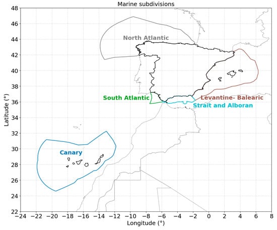
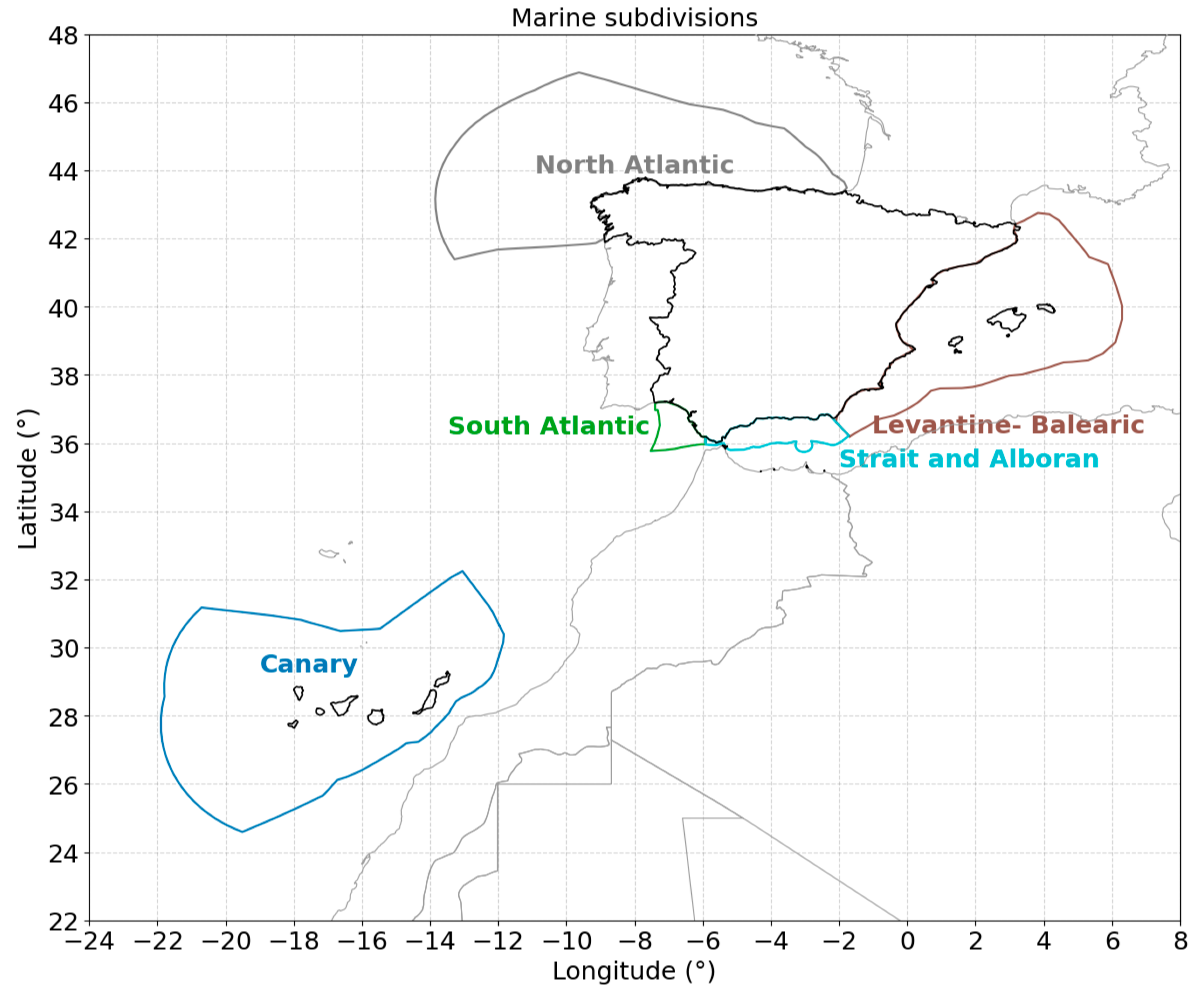
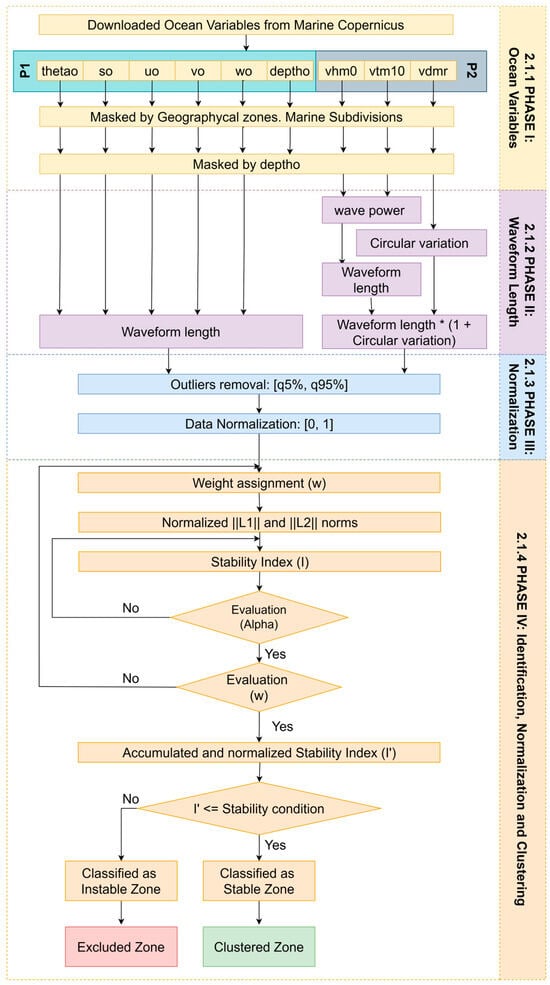
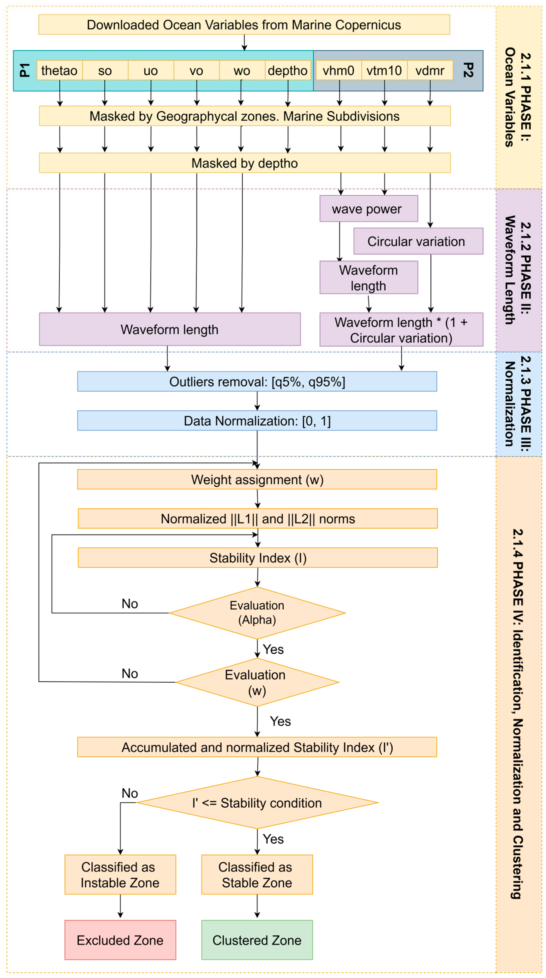
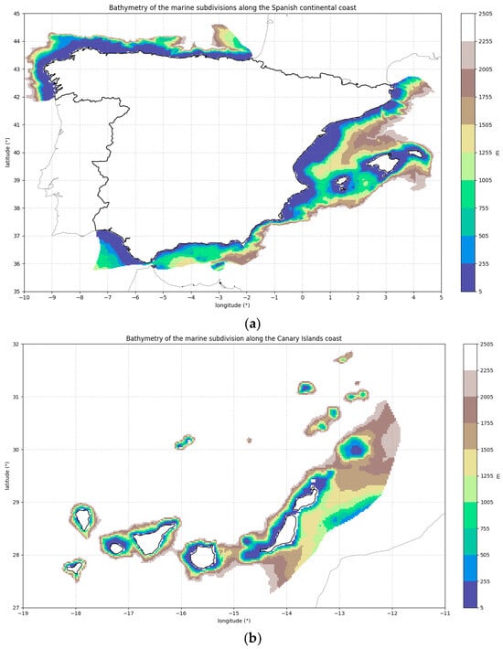
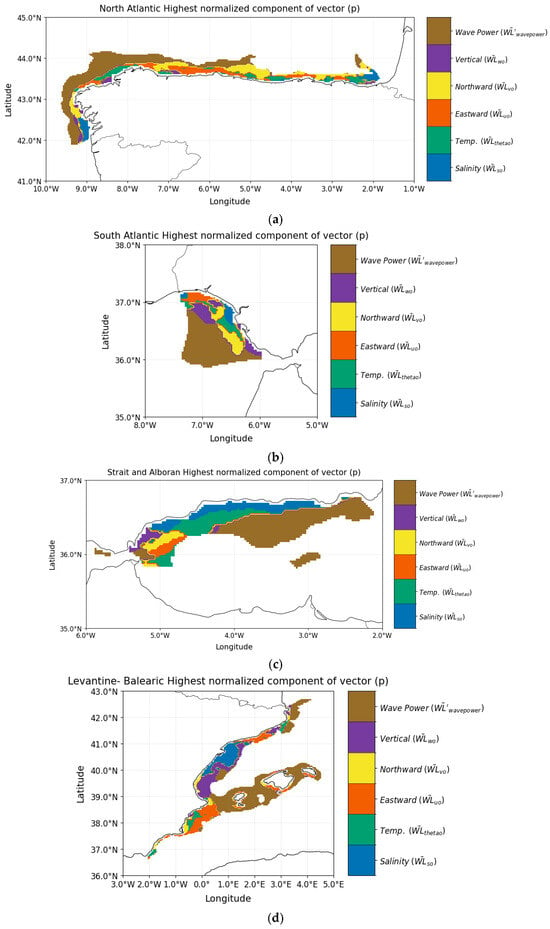
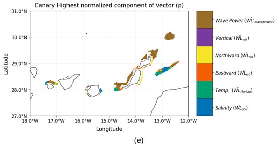
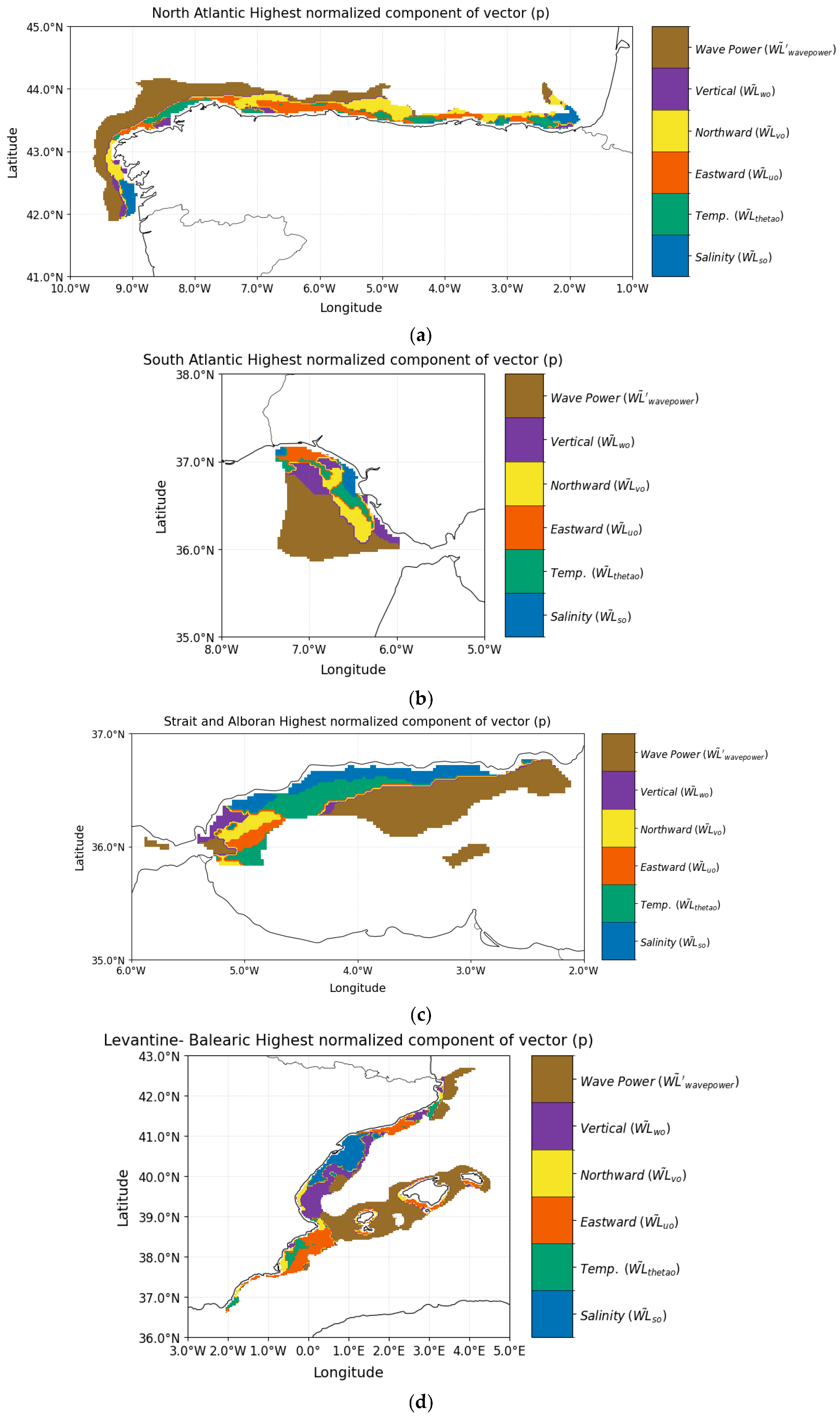
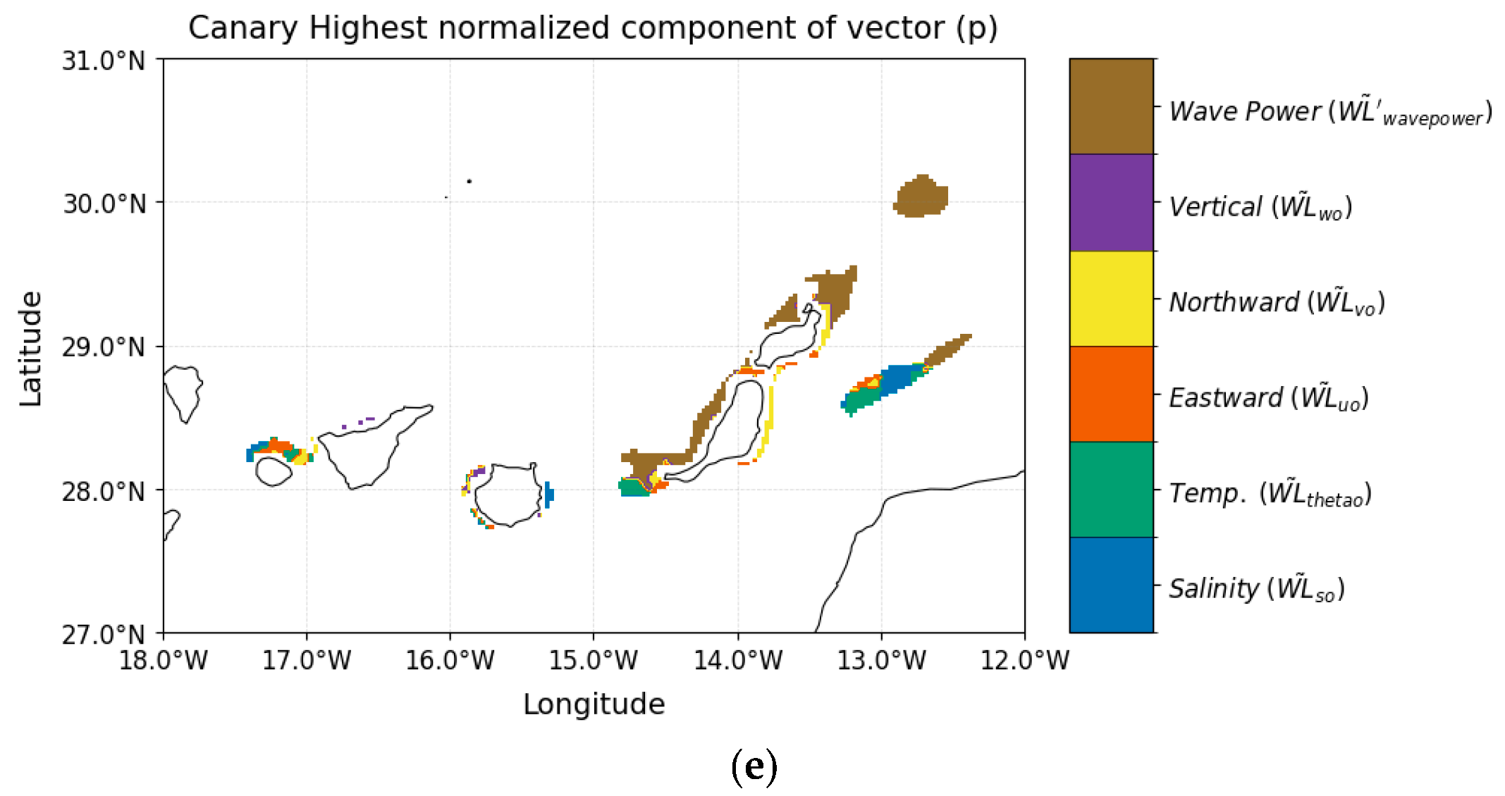
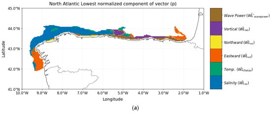
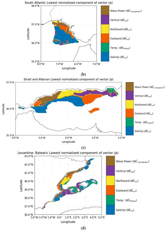
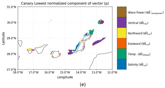
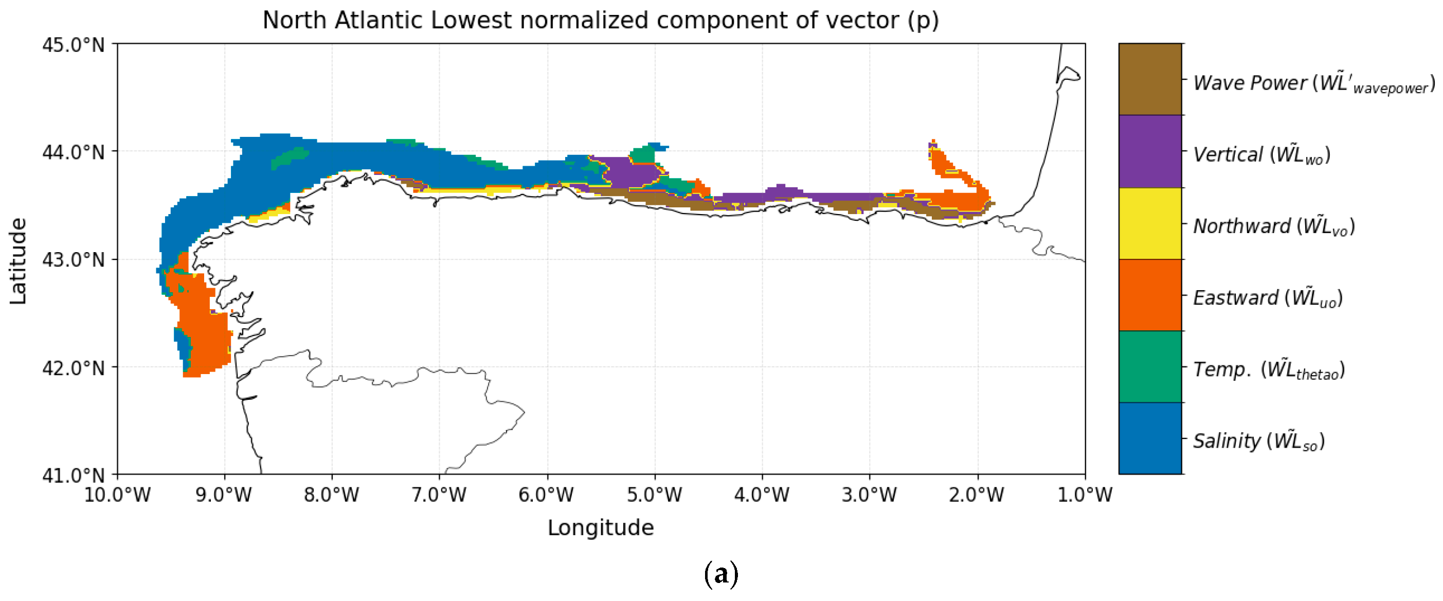
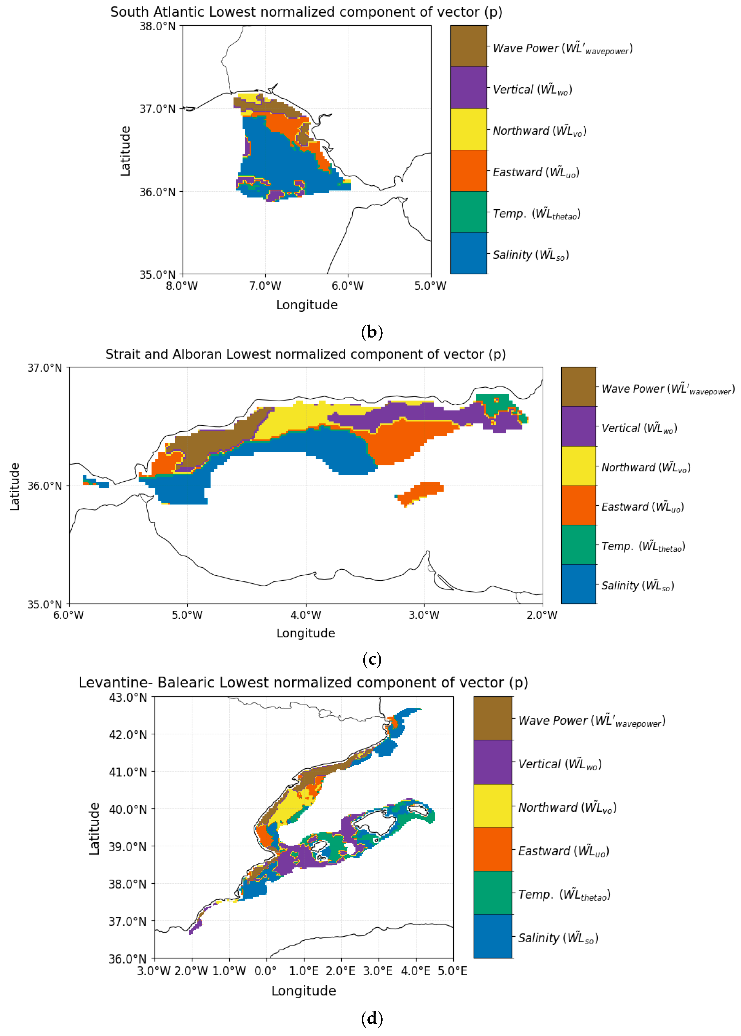
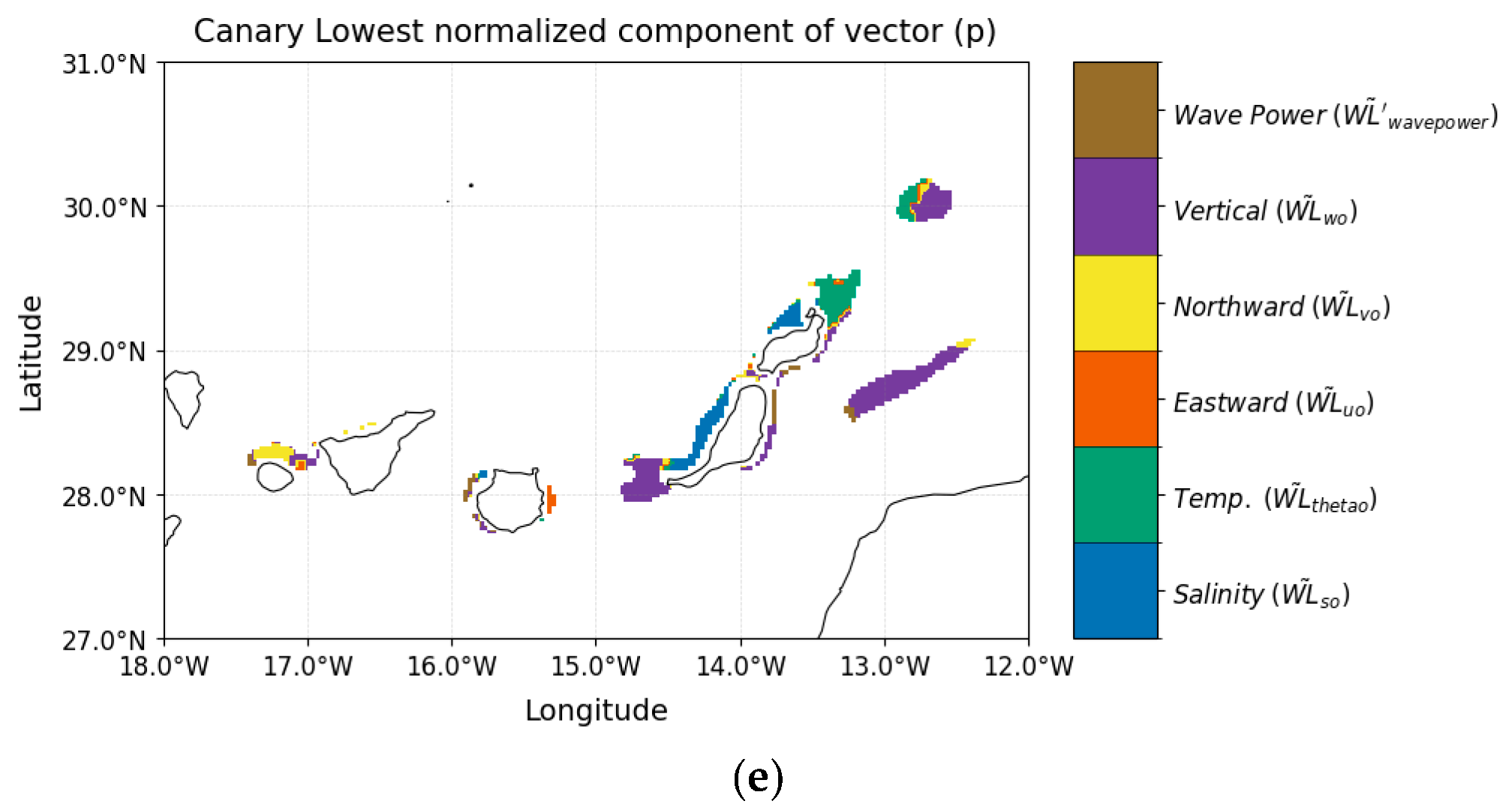
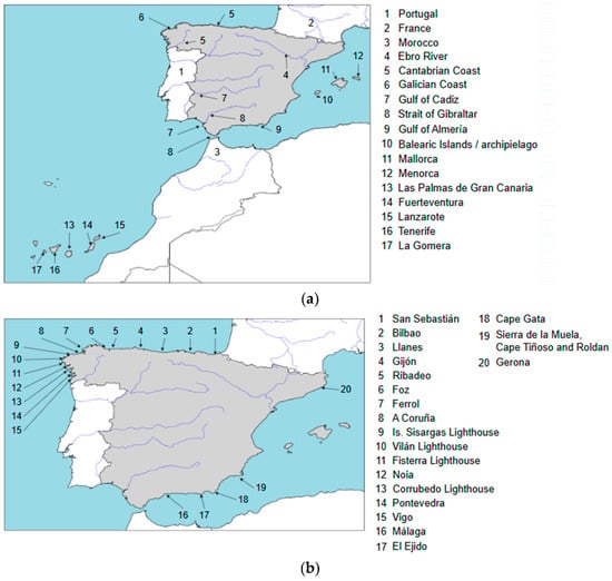
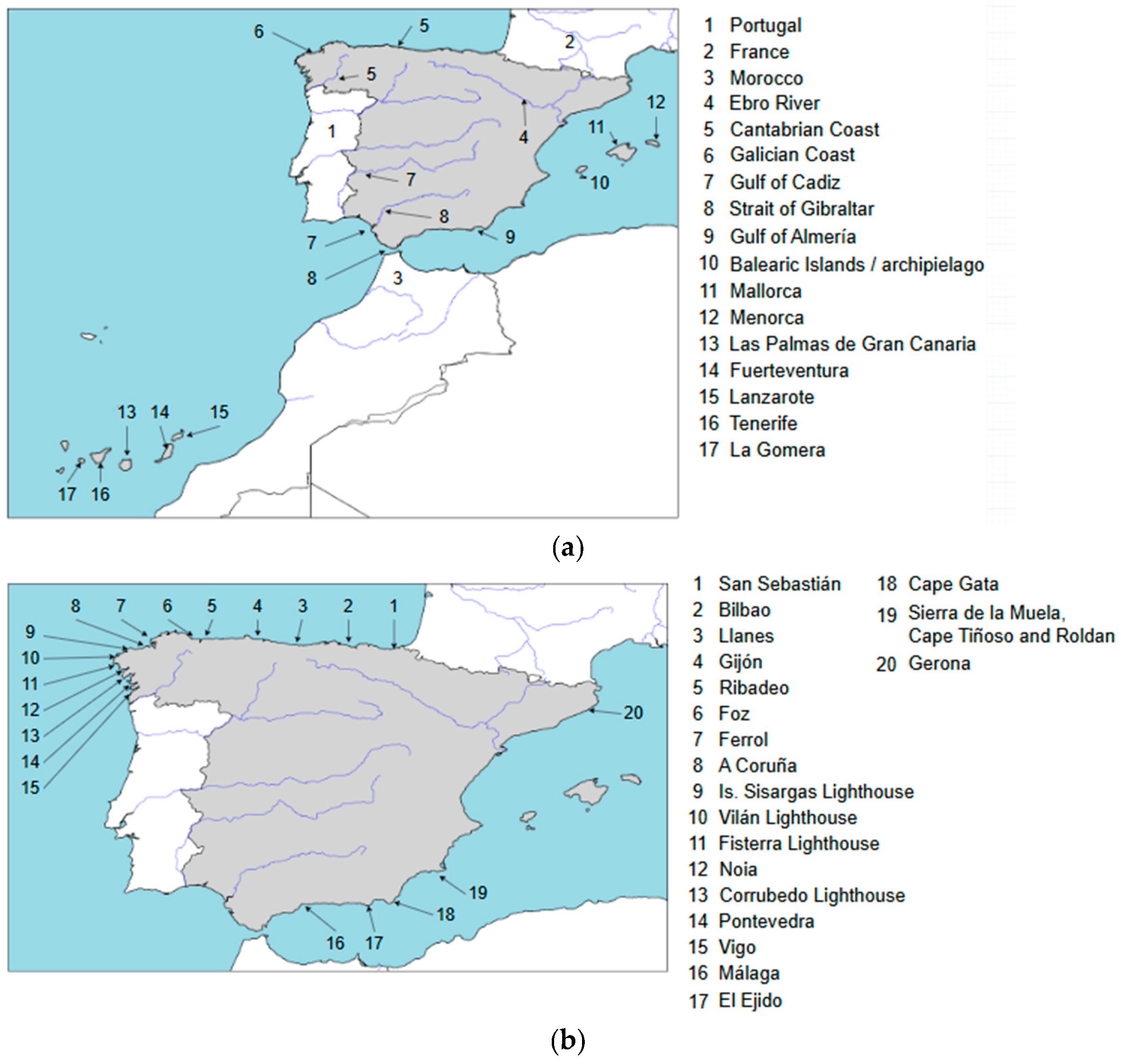
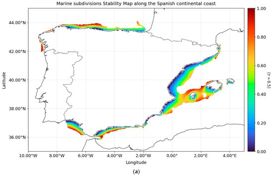
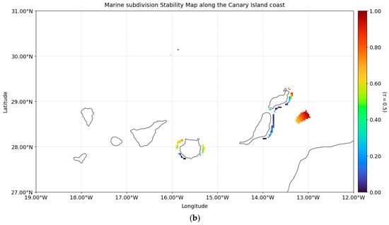
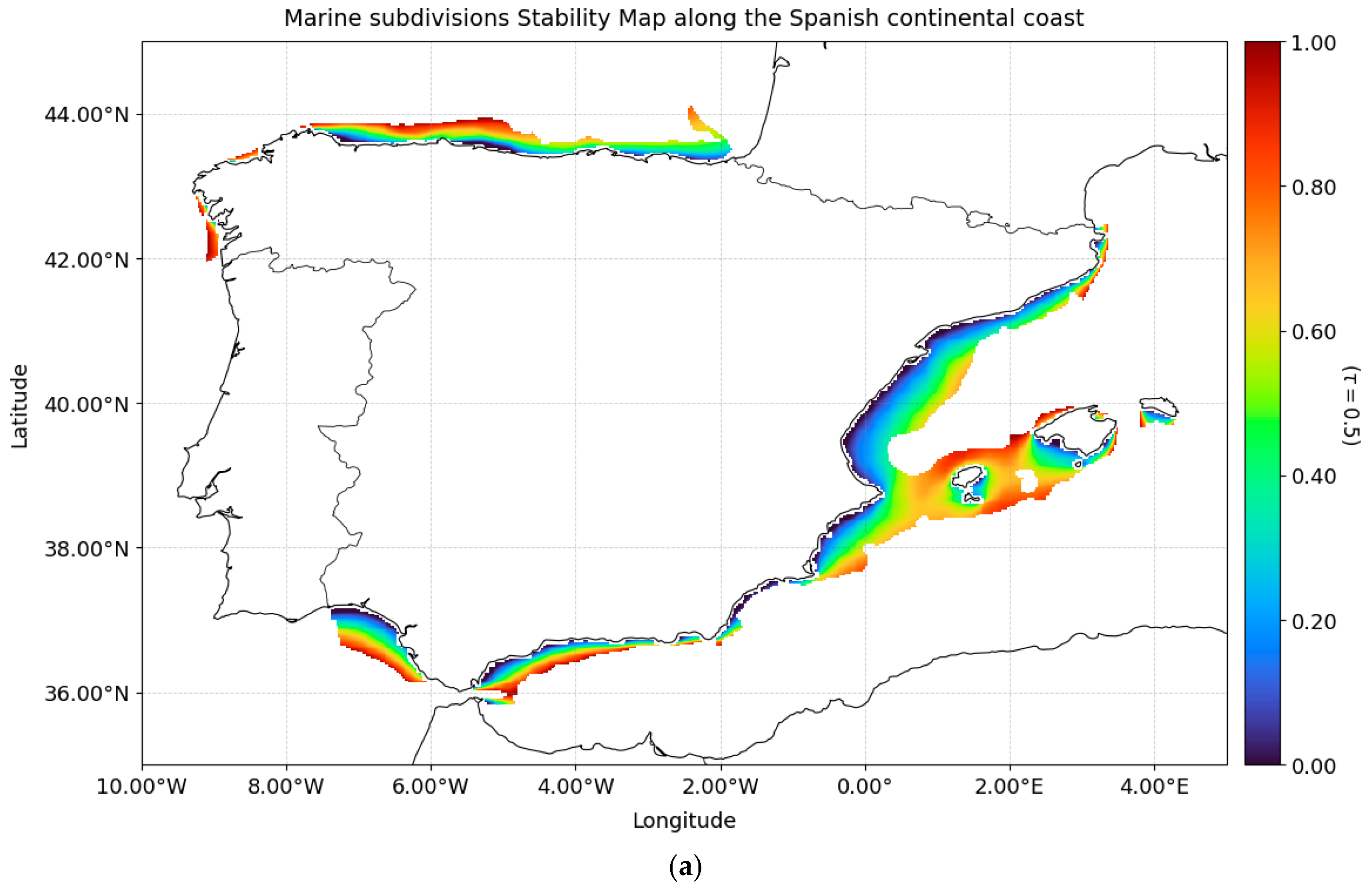
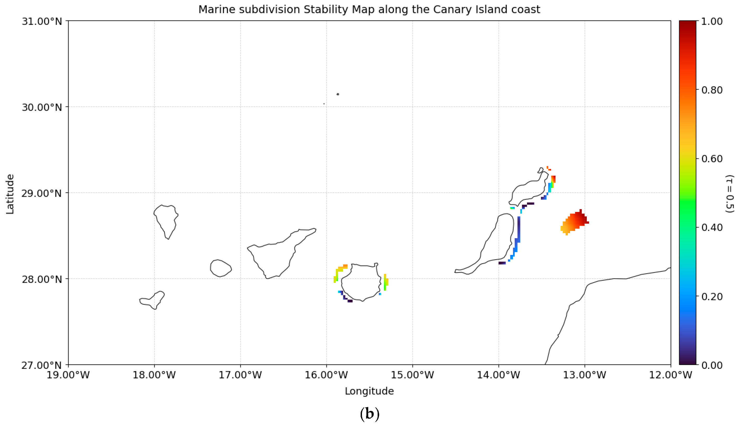
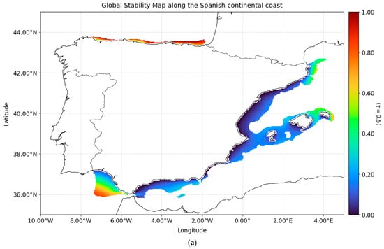
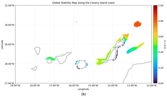
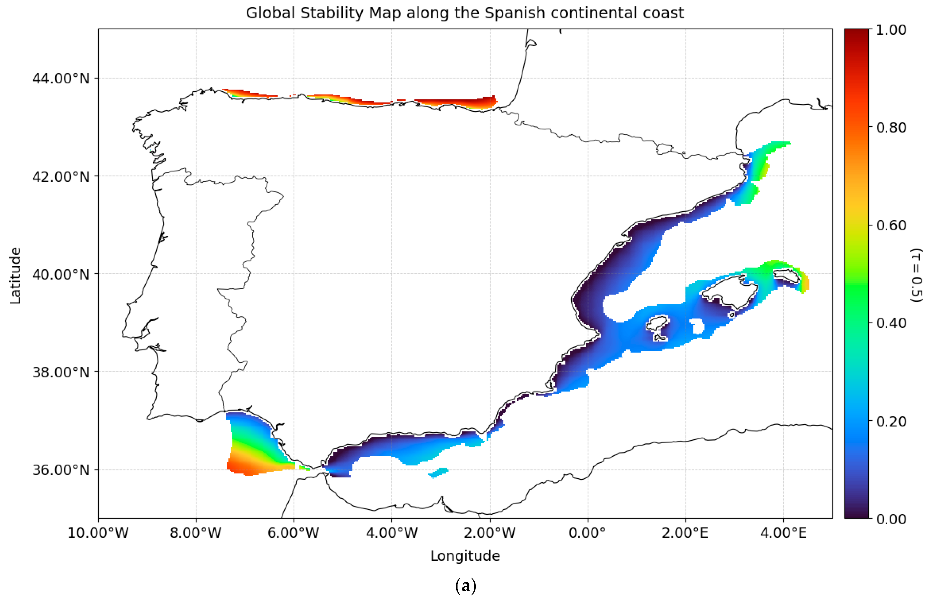
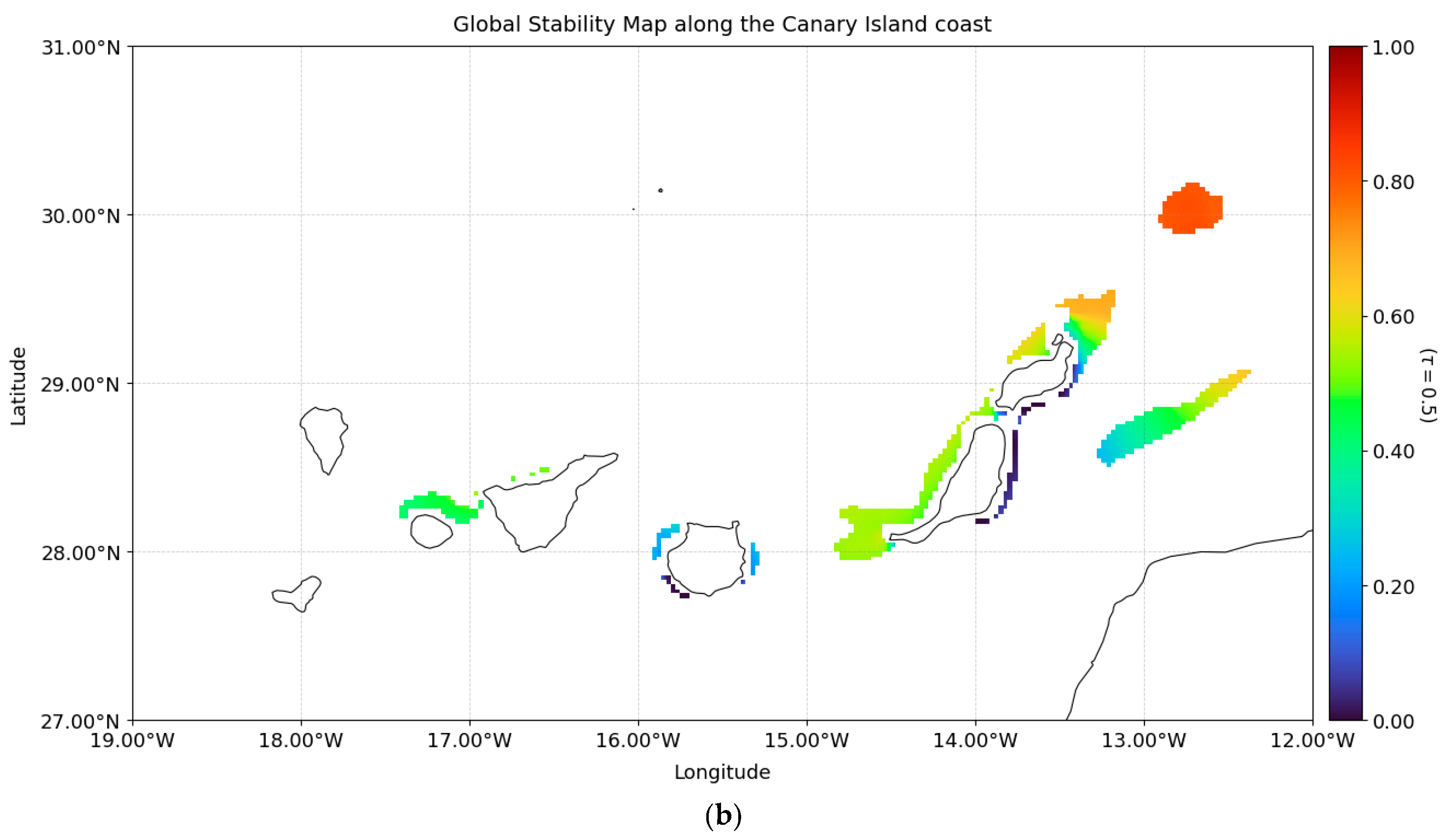
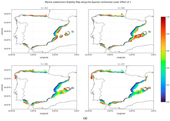
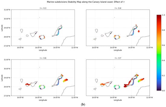
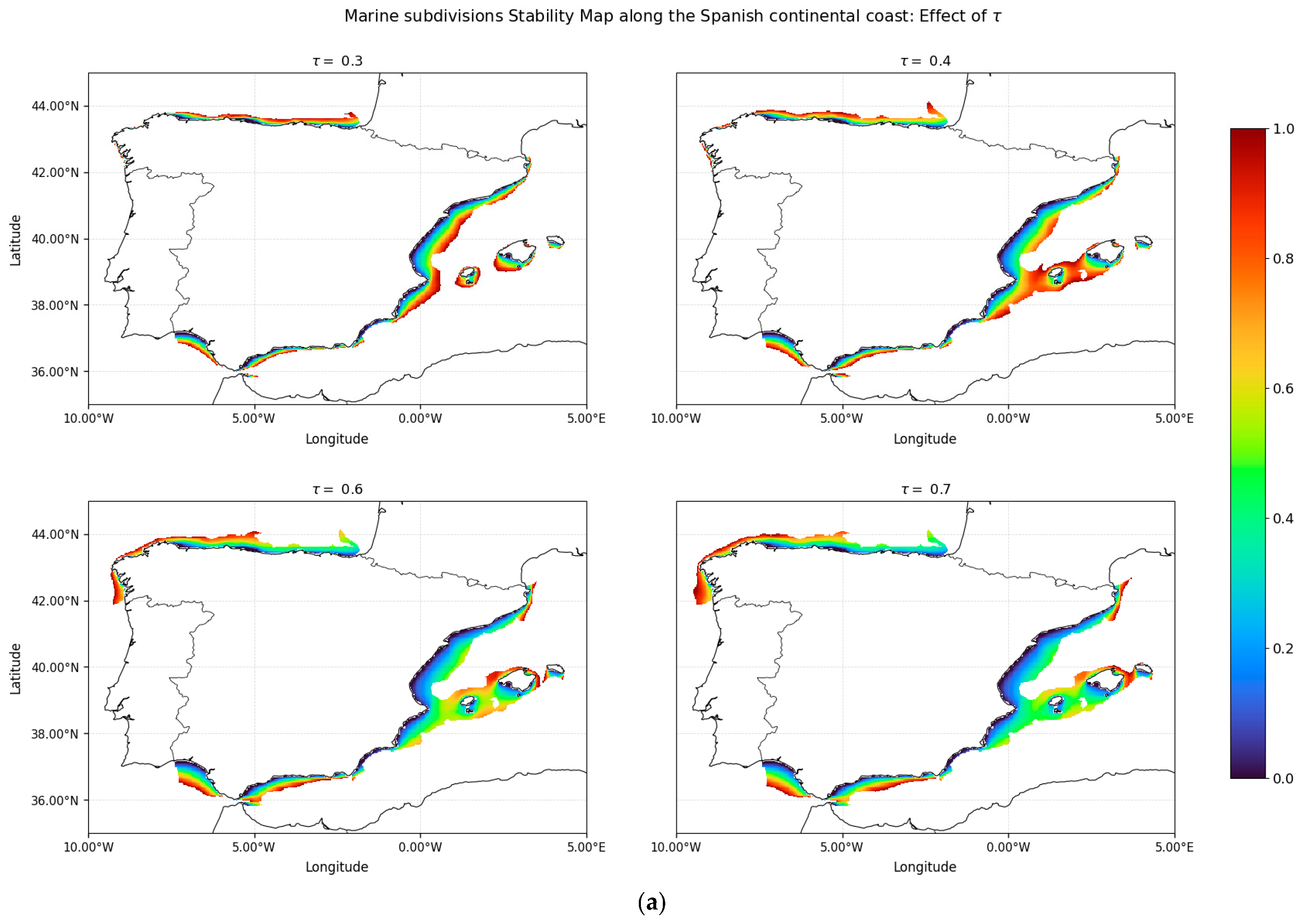
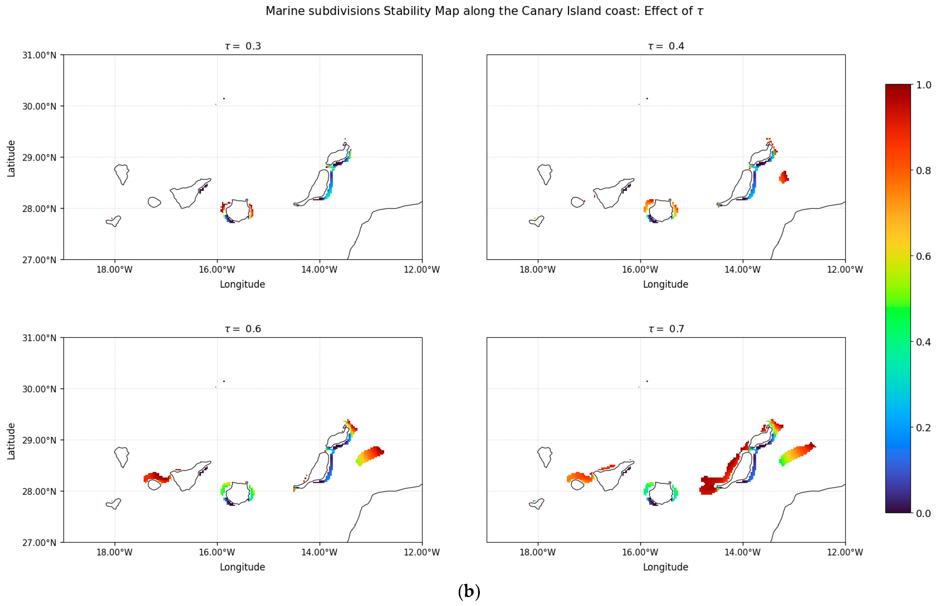

Disclaimer/Publisher’s Note: The statements, opinions and data contained in all publications are solely those of the individual author(s) and contributor(s) and not of MDPI and/or the editor(s). MDPI and/or the editor(s) disclaim responsibility for any injury to people or property resulting from any ideas, methods, instructions or products referred to in the content. |
© 2026 by the authors. Licensee MDPI, Basel, Switzerland. This article is an open access article distributed under the terms and conditions of the Creative Commons Attribution (CC BY) license.