


Highlights
Please indicate how your work links to systems science via your contributions to systems practice, theory, and or methodology.
- A set of dispatching heuristics and a genetic algorithm are developed for a hybrid flow shop scheduling problem that jointly incorporates lot streaming, no-wait, blocking, and sequence-dependent setup times, motivated by a real industrial problem.
- This study demonstrates how multiple interacting constraints jointly determine system behavior, capturing trade-offs that partial models would fail to reveal.
What are the main findings and/or the implications of the main findings?
- The genetic algorithm consistently yields superior schedules and near-optimal solutions on small instances, while the proposed dispatching heuristics achieve comparable quality within seconds, rendering them suitable for real-time scheduling decisions.
- The benefit of sequence optimization over a simple setup-minimizing rule varies non-monotonically with machine capacity and setup time magnitude, guiding managers on when capacity expansion or setup time reduction is most worthwhile.
Abstract
This study considers a 1-m-1 hybrid flow shop scheduling problem that simultaneously incorporates four practical constraints: lot streaming, no-wait, blocking, and sequence-dependent setup times. Although each of these characteristics has been studied individually in the literature, their joint consideration in a single HFS model has received little attention. The problem is motivated by a real-world order sequencing problem in insulation board manufacturing, where all four constraints arise simultaneously from the production process. To formally characterize the problem, we develop a mixed-integer programming formulation that captures all operational constraints. For practical-scale problems, we propose several dispatching heuristics that can obtain sufficiently good solutions within a short computation time. We further develop a genetic algorithm as an independent solution approach to obtain high-quality solutions close to the optimum within a reasonable computation time. Computational experiments on instances generated based on real insulation board production characteristics demonstrate that the proposed algorithms outperform a benchmark greedy rule, and sensitivity analyses reveal the effects of setup time magnitude and the number of parallel machines on scheduling performance.
1. Introduction
Efficient scheduling is a central requirement in industrial management, particularly in multi-stage production systems where limited resources, technological constraints, and product-dependent operations must be coordinated simultaneously. The hybrid flow shop (HFS) is a representative production layout for such systems and has been widely adopted in manufacturing industries such as paper, steel, textiles, chemicals, and semiconductor fabrication. An HFS consists of a series of processing stages, each containing one or more parallel machines, through which every job must pass in a fixed order while being processed by exactly one machine at each stage. As a generalization of both the flow shop scheduling problem and the parallel machine scheduling problem, the HFS captures the essential structure of many real-world production systems and has been extensively studied due to its theoretical significance and practical relevance [1]. Since even the simplest two-stage variant is NP-hard [2], heuristic and metaheuristic approaches are often required to obtain high-quality schedules within reasonable computation times.
In practice, real manufacturing systems impose operational constraints that extend well beyond the classical HFS setting. Four characteristics are particularly important in many production environments. First, lot streaming divides a job or lot into smaller sublots, allowing downstream stages to begin processing before the entire lot has completed the preceding stage. This enables overlap among stages and can significantly reduce makespan by improving resource utilization and reducing idle time [3]. Second, the no-wait constraint requires that a sublot move to the next stage immediately after completing the current stage. This condition arises when intermediate storage is unavailable or when product quality may deteriorate if waiting occurs [4]. Third, the blocking constraint occurs when a completed sublot cannot be released from the current machine because the downstream resource is unavailable. In such cases, the sublot remains on the current machine and prevents it from processing subsequent sublots, which is typical of zero-buffer or limited-buffer production systems [4]. Fourth, sequence-dependent setup times (SDSTs) arise when the setup required before processing a job depends on the job processed immediately beforehand. In such environments, sequencing decisions directly affect total setup time and therefore become inseparable from scheduling decisions [5]. Each of these characteristics has been studied in the scheduling literature, but their simultaneous consideration remains challenging because of their strong interactions.
Existing studies have generally focused on individual constraints or partial combinations of these features. For example, Wang et al. [6] studied an HFS problem with lot streaming and SDSTs, while Maciel et al. [7] considered blocking and SDSTs. However, studies that simultaneously incorporate lot streaming, no-wait, blocking, and SDSTs within a single HFS model are scarce. The interaction among these four constraints creates a scheduling structure that differs qualitatively from models considering only one or two of them. A sequence that performs well under a partial set of constraints may become infeasible or highly inefficient once the remaining constraints are also enforced. Therefore, algorithms designed for simpler HFS variants cannot be expected to perform effectively in fully constrained real-world settings, which motivates the development of a dedicated problem formulation and tailored solution methods.
This study addresses a real-world order sequencing problem arising in the production of insulation boards. The target production system is a three-stage 1-m-1 HFS consisting of a single machine at the first stage, multiple parallel machines at the second stage, and a single machine at the third stage. The problem requires determining the processing sequence of customer orders while simultaneously considering lot streaming, no-wait, blocking, and SDSTs. From an industrial management perspective, the problem is not merely to minimize makespan, but to coordinate setup-intensive operations, bottleneck resources, zero-buffer material flow, and order-level processing decisions under practical computational limits. A detailed description of the production process and the resulting scheduling characteristics is provided in Section 3.
To the best of our knowledge, no prior work has formulated or solved the 1-m-1 HFS scheduling problem under the simultaneous presence of lot streaming, no-wait, blocking, and SDSTs. This paper addresses this gap by developing an exact mathematical formulation and practical solution algorithms for a real-world constrained production scheduling problem. The main contributions of this study are as follows:
- We formally define a 1-m-1 HFS scheduling problem that simultaneously considers lot streaming, no-wait, blocking, and SDSTs, motivated by a real-world insulation board manufacturing process, and develop a mixed-integer programming (MIP) formulation.
- We propose three families of dispatching heuristics, including a setup-time-based greedy heuristic, rollout-based heuristics, and exchange-based heuristics, to obtain high-quality solutions rapidly for practical production scheduling.
- We develop a genetic algorithm (GA) with multiple selection and crossover operators to obtain improved makespan solutions within a reasonable computation time.
- We conduct computational experiments on instances generated based on real insulation board production characteristics, compare the proposed algorithms in terms of solution quality and computation time, and provide sensitivity analyses with respect to setup time magnitude and the number of parallel machines at the second stage.
The remainder of this paper is organized as follows: Section 2 reviews the relevant literature on HFS scheduling, lot streaming, no-wait and blocking constraints, and SDSTs. Section 3 describes the insulation board production process and presents the MIP formulation. Section 4 and Section 5 introduce the proposed dispatching heuristics and the genetic algorithm, respectively. Section 6 reports the computational experiments, sensitivity analyses, and managerial implications. Section 7 concludes this paper and discusses future research directions.
2. Literature Review
This section reviews studies related to the constrained hybrid flow shop scheduling problem considered in this paper. Since the basic concepts of the four main characteristics—lot streaming, no-wait, blocking, and sequence-dependent setup times (SDSTs)—were introduced in Section 1, this section focuses on how each characteristic has been addressed in the HFS scheduling literature, and how prior studies have combined them.
2.1. Hybrid Flow Shop Scheduling
The hybrid flow shop scheduling problem (HFSP) has been extensively studied because it represents a broad class of multi-stage manufacturing systems. Early review papers established the theoretical foundation and classification framework of HFSPs. Linn and Zhang [8] reviewed modeling and solution approaches, while Kis and Pesch [9] focused on exact solution methods for non-preemptive multiprocessor flow shop problems. Wang [10] classified HFSP solution methods into exact algorithms, heuristics, and artificial-intelligence-based approaches. Quadt and Kuhn [11], Ruiz and Vazquez-Rodriguez [1], and Ribas et al. [12] subsequently provided comprehensive taxonomies covering HFSP variants, constraints, and solution methods. More recent reviews by Lee and Loong [13] and Neufeld et al. [14] further summarized developments in flexible flow shop and multi-objective HFS research.
Due to the NP-hard complexity of HFSPs, exact methods are generally applicable only to small instances, whereas heuristic and metaheuristic approaches are widely adopted for industrial-scale problems. As manufacturing systems have grown more complex, the classical HFSP has been extended to incorporate practical constraints such as lot streaming, no-wait, blocking, sequence-dependent setup times, machine eligibility, and limited buffers.
2.2. HFS Scheduling with Lot Streaming
Lot streaming has been studied mainly in classical flow shop settings [3,15,16,17], but its extension to HFS environments is more complex because sublots must be coordinated across parallel machines within each stage. Early HFS lot-streaming studies therefore often focused on two-stage systems. Kim et al. [18] considered a two-stage HFS in which jobs are split into fixed-size lots for makespan minimization. Zhang et al. [19] studied a multi-machine first stage with a single second-stage machine, proposing heuristics to minimize mean completion time. Liu [20] developed exact and heuristic approaches for a similar setting with a predetermined number of sublots. Cheng et al. [21] addressed the joint determination of sublot number and size. Nejati et al. [22] investigated an assembly HFS with multiple machines at both stages using a hybrid GA and simulated annealing. Wang et al. [6] studied a two-stage paint manufacturing HFS with variable sublots and sequence-dependent setup times.
Multi-stage HFS with lot streaming has received comparatively less attention. Naderi and Yazdani [23] studied a general HFSP with sublots and SDSTs, minimizing total tardiness under fixed sublot sizes. Zhang et al. [24] proposed a modified migrating birds optimization algorithm for an HFSP with lot streaming to minimize total flow time. Chen et al. [25] addressed energy-efficient HFS scheduling with lot streaming, while Shao et al. [26] recently studied a distributed heterogeneous HFSP with lot streaming across factories of different capacities.
Across this body of work, lot streaming consistently improves production performance in HFS environments. However, the majority of these studies do not incorporate no-wait or blocking constraints alongside lot streaming. These constraints fundamentally alter sublot movement between stages and are characteristic of zero-buffer production systems such as the insulation board process studied here.
2.3. HFS Scheduling with No-Wait and Blocking Constraints
No-wait and blocking constraints have been widely studied in flow shop environments; Hall and Sriskandarajah [4] provided a foundational survey of scheduling problems involving both. In HFS settings, Sriskandarajah et al. [27] showed that the two-stage no-wait HFSP is NP-hard for makespan minimization. Sriskandarajah [28] subsequently developed heuristics with worst-case performance analysis for this problem. Xie et al. [29] proposed algorithms for minimizing makespan in a two-stage no-wait HFSP, and Cheng et al. [30] analyzed the computational complexity of two- and three-stage variants. Wang et al. [31] developed a genetic algorithm for a two-stage no-wait HFS, and Wang et al. [32] proposed a branch-and-bound approach for a related formulation. No-wait HFS models have also been applied to operating room scheduling [33,34], and Rabiee et al. [35] studied a no-wait HFS with unrelated parallel machines, machine eligibility, and SDSTs.
Blocking constraints in HFS environments have received somewhat less attention. Luo et al. [36] addressed a two-stage blocking HFS motivated by metalworking, while Missaoui et al. [37] proposed iterated greedy methods for a blocking HFS with due-date windows. Aqil et al. [38] studied a blocking HFS with SDSTs, and Qin et al. [39,40] developed iterated greedy algorithms for energy-efficient and distributed blocking HFS variants. Meng et al. [41] extended classical HFSP models to include no-wait and blocking as special cases within a unified MIP framework.
While no-wait and blocking constraints have both been studied in HFS settings, they are almost invariably treated in isolation or combined with at most one additional feature. No existing study examines a setting in which no-wait, blocking, and lot streaming coexist—the very combination that characterizes the insulation board process modeled in this paper.
2.4. HFS Scheduling with Sequence-Dependent Setup Times
Sequence-dependent setup times have been actively studied in HFS scheduling because changeover requirements vary with product type. Kurz and Askin [42] were among the first to address the HFSP with SDSTs, and subsequently proposed a random-key genetic algorithm for the same problem [43]. Zandieh et al. [44] introduced an immune algorithm and benchmarked it against the genetic algorithm. Subsequent work applied further metaheuristics, including agent-based GAs [45], simulated annealing [46,47], tabu search [48], and trajectory-based methods [49].
Several studies have combined SDSTs with one other HFS characteristic. Wang et al. [50], Jolai et al. [51], and Ramezani et al. [52] studied no-wait HFS with SDSTs. Aqil et al. [38] and Maciel et al. [7] considered HFS with blocking and SDSTs. Naderi and Yazdani [23], Nejati et al. [53], and Wang et al. [6] addressed lot streaming combined with SDSTs in HFS-related problems.
Taken together, these studies confirm the importance of SDSTs in practical HFS environments. Yet, in every case, SDSTs is paired with at most one of the other three characteristics—no-wait, blocking, or lot streaming. No existing study embeds SDSTs within a model that simultaneously imposes all three.
2.5. Learning-Based Approaches to HFS Scheduling
Beyond the heuristic and metaheuristic methods reviewed above, recent work has applied deep reinforcement learning (DRL) and graph neural networks (GNNs) to HFS scheduling. Zhao et al. [54] proposed an end-to-end DRL architecture based on a heterogeneous graph neural network for the general HFSP. Learning-based methods have also been applied to HFS variants involving individual characteristics considered in this paper: Zhao et al. [55] combined Q-learning with a cooperative meta-heuristic for no-wait flow-shop scheduling with SDSTs; Chen et al. [56] proposed a Q-learning-based hyper-heuristic for hybrid flow shop scheduling with lot streaming; and Wang et al. [57] developed a DRL policy network for the blocking hybrid flow shop scheduling problem.
These studies demonstrate that DRL and GNN-based methods can be effective when applied to HFS variants defined by one or two of the characteristics considered in this paper. Despite this progress, we adopted the dispatching heuristics and genetic algorithm (GA), rather than a learning-based approach, for two main reasons. First, designing a state representation and reward signal that correctly captures the interactions among lot streaming, no-wait, blocking, and SDSTs is a substantial undertaking in its own right, and no existing learning-based formulation provides a starting point for this specific combination of characteristics. Second, learning-based methods typically require a large number of training instances to generalize reliably, whereas the industrial process motivating this study is confidentiality-sensitive and does not provide access to a large historical dataset of real production schedules. Dispatching heuristics and a metaheuristic, neither of which requires training data and both of which generalize directly from the problem definition, are therefore better suited to the data availability constraints of our setting.
2.6. Research Gap
The preceding review shows that lot streaming, no-wait, blocking, and SDSTs have each been actively studied in HFS scheduling, and that several partial combinations have been explored. For example, lot streaming has been combined with SDSTs [6,23], no-wait with SDSTs [50,51,52], and blocking with SDSTs [7,38]. However, no prior study appears to have addressed all four characteristics simultaneously within a single HFS model.
This gap is not merely a matter of completeness. The four characteristics are coupled through a chain of sequencing and resource-release decisions that only closes when all four are present together: a sequencing choice made to reduce setup time determines how quickly sublots arrive at a shared downstream resource, blocking determines how long that resource stays occupied once congestion occurs, and the resulting delay in resource release feeds back into upstream sequencing decisions for later orders. A model that omits any one of the four characteristics breaks a link in this chain; so, a sequencing rule that appears optimal under a partial model need not remain so once all four constraints act together. Section 3.1 describes the specific mechanism by which this coupling arises in our production setting, and our sensitivity results in Section 6.5 confirm it empirically: the benchmark greedy rule, which sequences orders solely to minimize setup time, is competitive only when the number of Stage 2 machines is large enough to absorb the resulting congestion, and degrades sharply otherwise. Existing studies that combine at most two of the four characteristics cannot expose this trade-off, and algorithms developed for such partial models have no mechanism to account for it—which is the underlying reason a dedicated formulation and tailored heuristics are necessary here.
This study addresses this gap by formulating a 1-m-1 HFS scheduling problem that simultaneously incorporates lot streaming, no-wait, blocking, and SDSTs—a combination that, to the best of our knowledge, has not been jointly considered in the existing literature. The problem is motivated by a real insulation board manufacturing process, described in detail in the next section.
3. Problem Description and Mathematical Formulation
This section formally defines the scheduling problem studied in this paper. Section 3.1 describes the insulation board manufacturing process and introduces the problem structure and assumptions. Section 3.2 presents the mixed-integer programming (MIP) formulation.
3.1. Problem Description
3.1.1. Production Process
This study is motivated by a real-world scheduling problem encountered in the production of phenolic foam insulation boards. The insulation board is manufactured by forming a thermal core between two flexible facings. The production process consists of three sequential stages: foaming (Stage 1), curing (Stage 2), and cutting (Stage 3).
At Stage 1, raw boards are continuously fed into the line and a mixture of phenolic resin, catalyst, hardener, and blowing agent is sprayed onto each board through the nozzle of a foaming tank. At Stage 2, the foamed boards are held inside curing chambers under controlled temperature and humidity until the resin fully solidifies. Stage 2 consists of m parallel curing chambers, each of which can accommodate a fixed number of boards at a time. At Stage 3, the cured boards are precision-cut by a single cutting machine to the thickness and length specified in each customer order.
3.1.2. Orders and Sublots
The scheduling problem is to determine the processing sequence of a set of n customer orders so as to minimize the total makespan. Each order is characterized by the board thickness and quantity required by the customer, which together determine the processing times at each stage prior to scheduling.
Each order j is divided into smaller processing units called sublots, where each sublot corresponds to the portion of the order that occupies one curing chamber at Stage 2. The number of sublots is determined by the total board quantity and the chamber capacity, and order j thus consists of sublots . Because all curing chambers have the same capacity, sublots of the same order have identical sizes and identical processing times at every stage.
3.1.3. Operational Constraints
The three-stage process described above gives rise to all four characteristics considered in this study, as illustrated in Figure 1. We first describe the lot-streaming structure, which defines the sublot-level flow of each order, and then explain the stage-specific constraints imposed on this flow.
Figure 1.
Example Gantt chart of the insulation board production schedule.
Lot streaming: Because the curing stage is considerably longer than both the foaming and cutting stages, it represents the bottleneck of the production process. To improve overlap among successive stages and thereby reduce the overall makespan, each order is split into sublots that can be processed across multiple curing chambers. This lot-streaming structure allows the foaming, curing, and cutting operations of an order to proceed in an overlapping manner while requiring the sublot flow to be coordinated with the no-wait and blocking constraints. At Stage 3, orders are processed in the sequence determined by their Stage 2 completion times—that is, the order whose last sublot completes curing first is processed first at Stage 3. Sublots belonging to the same order are then processed consecutively.
No-wait constraint (Stage 1 → Stage 2): Once a sublot completes foaming at Stage 1, the foamed resin must immediately enter a curing chamber at Stage 2. Any delay between the two stages causes the resin to begin solidifying outside the chamber, compromising the structural integrity of the board. Accordingly, a sublot cannot wait between Stage 1 and Stage 2: the start time of each sublot at Stage 2 is fully determined by its completion time at Stage 1.
Blocking constraint (Stage 2 → Stage 3): There is no intermediate buffer between the curing chambers and the cutting machine. Once curing is complete, a sublot must wait inside its curing chamber until the cutting machine at Stage 3 becomes available to process it. During this waiting period, the curing chamber is occupied and cannot accept a new sublot. This constitutes the blocking constraint: a sublot that has completed Stage 2 blocks its curing chamber until Stage 3 can begin.
Sequence-dependent setup times (Stage 1): At the foaming stage, the setup time between consecutive orders depends on the difference in board thickness. A larger difference in thickness between the preceding and the following order requires a longer reconfiguration of the foaming equipment. Furthermore, for the same thickness difference, the setup time is longer when the following order has a larger thickness than the preceding one, because upsizing the board dimensions requires more careful adjustment than downsizing. Let denote the setup time incurred at Stage 1 when order k is processed immediately after order j.
3.1.4. Problem Summary
Using standard scheduling notation, the problem studied in this paper can be summarized as follows:
- The production process is a 1-m-1 HFS: Stage 1 and Stage 3 each have a single machine, and Stage 2 has m identical parallel machines ().
- There are n orders to be scheduled; order consists of sublots of equal size. All sublots of the same order have identical processing times at each stage.
- At Stage 1, a sequence-dependent setup time is incurred when order k is processed immediately after order j ().
- A no-wait constraint exists between Stage 1 and Stage 2: each sublot must move to Stage 2 immediately upon completing Stage 1.
- A blocking constraint exists between Stage 2 and Stage 3: a sublot that has completed Stage 2 must remain on its machine until the Stage 3 machine becomes available.
- All orders are available for processing at time zero. Preemption is not allowed.
The objective is to find an order sequence that minimizes the makespan .
3.2. Mathematical Formulation
The mathematical symbols, sets, parameters, and decision variables used in the formulation are summarized in Table 1 for reference.
Table 1.
Notation used in the problem formulation.
The scheduling problem described in Section 3.1 is formulated as the following mixed-integer program.
where M is a sufficiently large positive constant. The objective function (1) minimizes the makespan, i.e., the completion time of the last sublot processed across all orders. Constraint (2) ensures that the completion time of the first sublot of each order at Stage 1 is at least its processing time. Constraint (3) enforces sequential processing of the sublots belonging to the same order at Stage 1: sublot cannot complete before sublot l has finished. Constraint (4) captures the sequence-dependent setup time between consecutive orders at Stage 1. If order j precedes order k (i.e., ), the first sublot of order k cannot begin until the last sublot of order j has completed and the setup time has been served; otherwise, the constraint is relaxed by the big-M term.
Constraint (5) enforces the no-wait condition between Stage 1 and Stage 2. When sublot l of order j is assigned to machine i at Stage 2 (i.e., ), its completion time at Stage 2 equals its Stage 1 completion time plus the Stage 2 processing time, allowing for no idle time between the two stages. When , the big-M term renders the constraint inactive. Constraint (6) ensures that on each machine at Stage 2, consecutive sublots of the same order are processed sequentially: if both sublot l and sublot of order j are assigned to machine i, sublot cannot begin before sublot l has finished. Constraint (7) ensures that on each machine at Stage 2, the sublot of order k cannot start before the sublot of order j has finished, provided that both sublots are assigned to the same machine i and order j precedes order k at Stage 1.
Constraint (8) enforces the blocking condition between Stage 2 and Stage 3. The start time of sublot of order k on machine i at Stage 2 must be no earlier than the start time of sublot l of order j at Stage 3, whenever both sublots are on the same Stage 2 machine and order j precedes order k at Stage 3 (i.e., ). This ensures that sublot l has vacated the Stage 2 machine before sublot can begin curing, reflecting the zero-buffer blocking constraint. The coefficient arises because three binary variables appear in the activation term. Constraint (9) ensures that a sublot cannot begin processing at Stage 3 until its Stage 2 processing is complete. Constraint (10) enforces sequential processing of sublots of the same order at Stage 3. Constraint (11) determines the processing order of orders at Stage 3: if order j precedes order k at Stage 3 (i.e., ), the first sublot of order k cannot start until the last sublot of order j has finished. Constraint (12) links the Stage 3 processing sequence to the Stage 2 completion times of the last sublots of consecutive orders. Together with constraint (11), this prevents infeasible schedules in which a Stage 2 machine would be required to release a sublot before the preceding order has completed Stage 3.
Constraints (13) and (14) ensure that for every pair of distinct orders, exactly one precedes the other at Stage 1 and Stage 3, respectively. Constraint (15) ensures that each sublot is assigned to exactly one machine at Stage 2. Constraint (16) defines the makespan as the maximum completion time of the last sublot over all orders. Constraints (17) and (18) specify the domains of the binary decision variables.
4. Dispatching Heuristics
Since the 1-m-1 HFS scheduling problem with lot streaming, no-wait, blocking, and SDSTs is NP-hard, exact solution via the MIP formulation in Section 3.2 is feasible only for small instances. For practical production environments where schedules must be generated quickly, we propose three families of dispatching heuristics: a greedy heuristic, an exchange heuristic, and a rollout heuristic. All three heuristics operate on the order sequence and evaluate candidate schedules using a common schedule evaluation function, COMPUTESCHEDULE(K), which computes the makespan of a given sequence by simulating the 1-m-1 HFS under the no-wait, blocking, SDSTs, and lot-streaming constraints defined in Section 3.1.
4.1. Greedy Heuristic
The greedy heuristic constructs an order sequence by exploiting the dominant role of SDSTs at Stage 1. As noted in Section 3.1, the setup time at Stage 1 decreases as the thickness difference between consecutive orders diminishes, and the asymmetry of setup times means that processing a thinner order immediately after a thicker one incurs less setup time than the reverse. Because Stage 2 is the bottleneck of the production process and typically determines the makespan, minimizing total setup time at Stage 1 directly reduces idle time propagation into Stage 2.
The greedy heuristic therefore sorts all orders in descending order of board thickness.
This sorting strategy minimizes the total SDSTs at Stage 1 by ensuring that the thickness difference between consecutive orders is small and that the asymmetric setup penalty associated with a thicker order following a thinner order is avoided. When the number of Stage 2 machines m is sufficiently large to prevent bottlenecks at Stage 1, this rule produces an optimal or near-optimal schedule. The resulting sequence serves as the initial solution for the exchange and genetic algorithm described in Section 4.2 and Section 5, respectively.
4.2. Exchange Heuristic
The exchange heuristic is a local-search procedure that improves a given initial sequence by iteratively swapping pairs of orders. Starting from the given sequence, the algorithm repeatedly examines pairwise swaps and applies the swap that yields the greatest reduction in makespan, continuing until no improving swap exists. Two variants are proposed: the 2-EX heuristic and the Grouped 2-EX heuristic.
4.2.1. 2-EX Heuristic
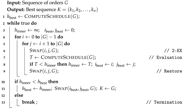
The 2-EX heuristic performs pairwise exchange over all pairs of orders in the current sequence. At each iteration, every pair with is examined by temporarily swapping orders at positions i and j in the sequence G, evaluating the resulting makespan via COMPUTESCHEDULE(G), and then restoring the original order. The swap that yields the minimum makespan is recorded. If is strictly less than the current best makespan , the swap is permanently applied and the search continues; otherwise, the algorithm terminates. The pseudocode is given in Algorithm 1.
| Algorithm 1: 2-EX heuristic. |
 |
4.2.2. Grouped 2-EX Heuristic
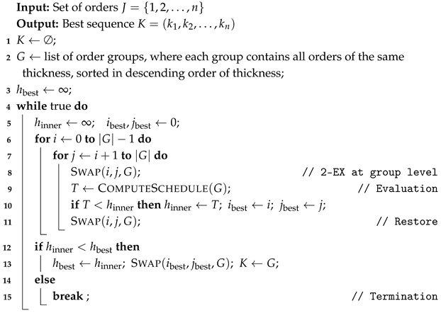
The Grouped 2-EX heuristic applies the 2-EX exchange logic at the level of thickness groups rather than individual orders. The key observation is that, under SDSTs, orders of the same thickness incur zero setup time between them; so, their relative order within a group does not affect the total setup time at Stage 1. The algorithm therefore first groups orders by board thickness and sorts the groups in descending order of thickness to form the initial sequence G. It then applies pairwise swaps between adjacent groups, evaluating the resulting makespan for each group-level swap. The swap that most reduces makespan is applied, and the process repeats until no further improvement is possible. The pseudocode is given in Algorithm 2.
| Algorithm 2: Grouped 2-EX heuristic. |
 |
4.3. Rollout Heuristic
The rollout heuristic is a sequential constructive procedure rooted in the rollout framework of Bertsekas and Castanon [58], which evaluates each candidate decision at a given stage by estimating its downstream cost using a base policy, rather than committing greedily. The approach has been successfully applied to a variety of scheduling problems [59,60,61,62], including those with blocking and no-wait constraints. We propose two variants: the basic rollout heuristic and the two-step rollout heuristic, both of which rely on the Base heuristic described below as their internal evaluation policy.
4.3.1. Basic Rollout Heuristic
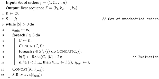
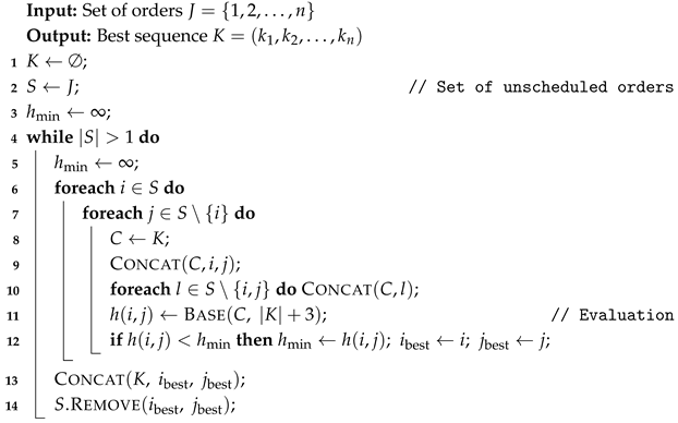
The rollout heuristic builds the sequence one order at a time. At each step, every unscheduled order is tentatively placed next in the partial sequence K, and the cost of this decision is estimated by appending the remaining orders via the Base heuristic and computing the resulting makespan. The order that leads to the minimum estimated makespan is permanently added to K and removed from S. This process repeats until all orders are scheduled. The pseudocode is given in Algorithm 3.
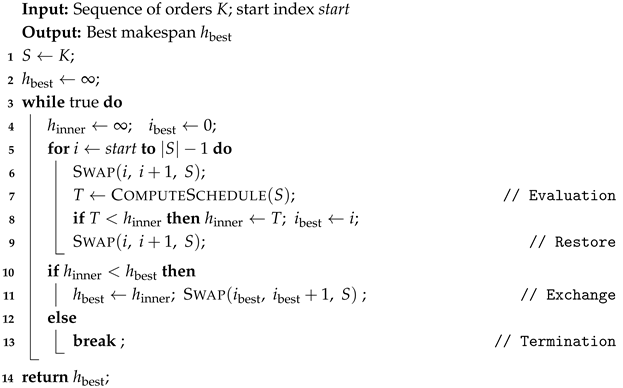
The evaluation step of Algorithm 3 invokes BASE (Algorithm 4), whose role is to estimate the cost-to-go from a partial sequence C in which the first positions are already fixed by the orders placed in K. Rather than accepting the arbitrary arrangement of the unscheduled orders appended in the preceding lines, the Base heuristic refines the remaining suffix of C by repeatedly applying pairwise adjacent exchanges until no further improvement in makespan is possible, and returns the resulting makespan.
| Algorithm 3: Rollout heuristic. |
 |
Specifically, given a sequence C and a starting index start, the base heuristic scans all adjacent pairs in the suffix , temporarily swaps them, evaluates the resulting makespan via COMPUTESCHEDULE, and restores the original order. The adjacent swap yielding the greatest reduction is applied, and the scan repeats. The algorithm terminates when a full scan produces no improving swap, and returns the best makespan found. Because the base heuristic is invoked repeatedly inside the rollout loops, its computational efficiency directly controls the overall running time of the rollout heuristics. Using adjacent swaps (rather than all-pair swaps as in 2-EX) keeps each base heuristic call inexpensive while still providing a meaningful quality signal for the rollout evaluation. The pseudocode is given in Algorithm 4.
| Algorithm 4: Base heuristic: BASE. |
 |
4.3.2. Two-Step Rollout Heuristic
The two-step rollout heuristic extends the basic rollout by fixing two orders simultaneously at each iteration rather than one. At each step, every ordered pair of distinct unscheduled orders is tentatively appended to K, and the cost is estimated via BASE (Algorithm 4). The pair that minimizes the estimated makespan is permanently added to K and both orders are removed from S. Although evaluating all ordered pairs increases the computational effort relative to the basic rollout, it enables a deeper lookahead and typically yields solutions of higher quality. The pseudocode is given in Algorithm 5.
| Algorithm 5: Two-step rollout heuristic. |
 |
5. Genetic Algorithm
Although the dispatching heuristics proposed in Section 4 produce schedules rapidly, their solution quality is limited by the greedy nature of the search. To obtain higher-quality solutions within a reasonable computation time, we additionally propose a genetic algorithm (GA). The GA evolves a population of permutation-encoded chromosomes over multiple generations through selection, crossover, mutation, and elitist replacement. The overall procedure follows the sequence population initialization → selection → crossover → mutation → next-generation construction → termination check.
5.1. Encoding and Initialization
Each chromosome is encoded as a permutation vector of the n orders, representing the processing sequence at Stage 1. The fitness of a chromosome is evaluated by COMPUTESCHEDULE, with a smaller makespan corresponding to higher fitness.
The initial population consists of chromosomes generated as random permutations of the order set J. The population size is set proportional to n to ensure that the search space is adequately explored as the number of orders grows. Because the number of feasible permutations grows factorially with n, scaling Q linearly with n provides a reasonable balance between solution diversity and computation time. Preliminary experiments on a subset of the problem instances used in the computational study (Section 6), with all other GA parameters fixed at the values reported in Section 5.6, showed that varying the population-size multiplier alone (i.e., ) from 25 to 200 changes the average improvement over GRD by only about 0.25 percentage points, while computation time increases from approximately 7 s to approximately 241 s; the multiplier of 100 used throughout this paper balances solution quality with computation time.
5.2. Selection
The selection step chooses parent chromosomes from the current population to undergo crossover. We evaluated three selection methods—pairing selection [63], proportional roulette wheel selection [64], and rank-based roulette wheel selection [65]—and adopted rank-based roulette wheel selection in the final GA based on its best performance in preliminary experiments. Detailed results of these preliminary experiments are presented in Section 6.2.
In rank-based roulette wheel selection, all chromosomes in the current population are ranked in ascending order of makespan (rank 1 for the smallest makespan), and a selection probability proportional to rank is assigned to each chromosome. The fitness of chromosome i with rank among Q chromosomes is defined as follows:
where is the selective pressure parameter. A chromosome with rank receives the highest fitness value , while one with rank receives . When approaches 1.0, selection probabilities become nearly uniform, promoting diversity; when approaches 2.0, higher-ranked chromosomes are strongly favored. We set to balance exploitation of high-quality solutions with maintenance of population diversity. Preliminary experiments on the problem instances used in the computational study (Section 6), with all other GA parameters fixed at the values reported in Section 5.6, showed that varying alone over the 1.0–2.0 range changes the average improvement over GRD by less than 0.1 percentage points, confirming that GA performance is not sensitive to this parameter.
5.3. Crossover
The crossover step combines two selected parent chromosomes to produce two offspring chromosomes. We evaluated seven crossover operators: three classical operators— Partially Mapped Crossover (PMX), Modified Order Crossover (MOC), and Order Crossover (OX1) [66]—and four building-block-based operators designed to preserve meaningful partial orderings shared between parents—Similar Job Order Crossover (SJOX), Similar Job 2-Point Order Crossover (SJ2OX), Similar Block Order Crossover (SBOX), and Similar Block 2-Point Order Crossover (SB2OX) [67,68]. Preliminary experiments across all test scenarios showed that SB2OX achieved the highest average improvement over the greedy heuristic, and it was therefore adopted in the final GA. Detailed results of these preliminary experiments are presented in Section 6.2.
SB2OX is based on the concept of a building block, defined as a sequence of at least two consecutive genes that have identical values at the same positions in both parent chromosomes and . The operator proceeds in three steps, as illustrated in Figure 2.
Figure 2.
Illustration of the SB2OX crossover operator applied to parent chromosomes and . (a) Step 1: building blocks shared by and (highlighted in blue) are inherited directly by offspring and at their shared positions. (b) Step 2: two cut points are selected and the segment between them is copied from the opposite parent (, highlighted in green; , highlighted in orange); positions filled in Step 1 are not overwritten. (c) Step 3: the remaining unfilled positions are completed by reading sequentially through the same parent ( for , for ), skipping genes already present in the offspring.
In Step 1 (building block inheritance), up to two building blocks are identified from and and copied directly into the offspring and at their shared positions, preserving common partial orderings between the two parents. If no building block is shared between the two parents, Step 1 contributes no positions, and the offspring are generated entirely by Steps 2 and 3.
In Step 2 (two-point crossover), two random cut points are selected in and . For offspring , the segment between the cut points is copied from ; for offspring , the corresponding segment is copied from . Genes already placed in Step 1 retain their positions and are not overwritten.
In Step 3 (filling the remaining positions), the positions left unfilled after Steps 1 and 2 are completed by reading through the opposite parent sequentially and inserting genes not yet present in the offspring. Specifically, the remaining positions of are filled from , and those of are filled from , skipping any gene already assigned.
Step 1 exploits convergent partial orderings accumulated in the population, while Steps 2 and 3 introduce recombination diversity, achieving a balance between exploitation and exploration.
5.4. Mutation
Mutation introduces random perturbations into the population to maintain diversity and prevent premature convergence. For each chromosome in the population, mutation is applied with probability . When triggered, swap operations are performed, where , so that approximately of the genes are displaced. Each swap exchanges two randomly chosen positions in the chromosome. Using the same instances as in Section 5.2, we also examined the sensitivity of the mutation parameters r and , with all other GA parameters fixed at the values reported in Section 5.6. Jointly varying r and over the 0.1–0.5 range changed the average improvement over GRD by less than 0.2 percentage points, though computation time increased with both parameters; the smaller values used here were retained accordingly.
5.5. Next-Generation Construction and Termination
After applying selection, crossover, and mutation to the current population of Q chromosomes, Q offspring chromosomes are produced. The chromosomes comprising the current population and the offspring are merged, and the best Q chromosomes by makespan are retained to form the next generation. This elitist replacement strategy ensures that the best solutions found are never discarded.
The GA terminates when the average improvement in makespan between consecutive generations falls below a threshold relative to the greedy heuristic solution. Formally, the termination condition is:
where is the makespan of chromosome i at generation t and is the makespan of the greedy heuristic solution. This criterion stops the GA once the population has effectively converged and further improvement becomes negligible.
5.6. Parameter Summary
Table 2 summarizes the parameter settings of the proposed GA.
Table 2.
Parameter settings of the proposed genetic algorithm.
6. Computational Experiments
This section presents computational experiments to evaluate the performance of the proposed dispatching heuristics and genetic algorithm.
6.1. Instances
Test instances were generated randomly to reflect the characteristics of the real insulation board production process described in Section 3.1. The numerical values used in the instances were scaled so as not to correspond directly to any actual production data, and units are omitted throughout.
Each order is assigned a board thickness drawn uniformly at random from nine discrete levels: . The processing times of a sublot at each stage are determined by the board thickness of the corresponding order. Specifically, the Stage 1 (foaming) and Stage 3 (cutting) processing times are inversely proportional to thickness, while the Stage 2 (curing) processing time is directly proportional to thickness. The resulting processing time ranges are at Stage 1, at Stage 2, and at Stage 3, with processing times drawn from a uniform distribution over the corresponding interval at each stage. The number of sublots per order is sampled from a zero-truncated Poisson distribution with mean . The setup time at Stage 1 is determined by the thickness difference between consecutive orders j and k, as described in Section 3.1. The thickness difference is partitioned into intervals of width 5, and the setup time increases by 4 for each interval: for a difference of 1–5, for 6–10, and for 11–15, up to a maximum of for a difference of 21–25. In addition, when the following order k has a greater thickness than the preceding order j (i.e., an upward thickness change), the setup time is multiplied by a factor of 1.2, reflecting the asymmetric reconfiguration cost described in Section 3.1.
Scenarios are defined by varying two factors: the number of Stage 2 machines and the number of orders . The full factorial combination yields 30 scenarios in total. Because the GA incorporates stochastic elements in population initialization, selection, crossover, and mutation, we generate 10 independent random instances per scenario, yielding 300 instances in total. Algorithm performance is reported as the average improvement over the 10 instances within each scenario.
6.2. Preliminary Experiments on the Selection Method and Crossover Operator
Before finalizing the genetic algorithm described in Section 5, we conducted preliminary computational experiments to select the selection method and crossover operator used in the final GA from among the candidates introduced in Section 5.2 and Section 5.3. These experiments used the 300 random instances introduced above. All other GA parameters were fixed at the values reported in Section 5.6; only the selection method or the crossover operator was varied at a time.
We first compared the three candidate selection methods—pairing selection, proportional roulette wheel selection, and rank-based roulette wheel selection. For each selection method, the GA was run with each of the seven candidate crossover operators (PMX, MOC, OX1, SJOX, SJ2OX, SBOX, and SB2OX) on all 300 instances, yielding evaluations per selection method. Figure 3 shows the distribution, over these 2100 evaluations, of the percentage improvement in makespan over the GRD heuristic achieved by the GA under each selection method.
Figure 3.
Distribution of the percentage improvement over GRD achieved by the GA, by selection method (2100 evaluations per method: 7 crossover operators × 300 random instances).
As shown in Figure 3, the three selection methods achieve broadly similar improvement distributions. Rank-based roulette wheel selection achieved the highest average improvement among the three and was therefore adopted as the selection method of the proposed GA.
We then compared the seven candidate crossover operators using the same procedure, fixing each crossover operator in turn and applying all three selection methods to the 300 instances, yielding evaluations per crossover operator. Figure 4 shows the resulting improvement distributions.
Figure 4.
Distribution of the percentage improvement over GRD achieved by the GA, by crossover operator (900 evaluations per operator: 3 selection methods × 300 random instances).
SB2OX and SJ2OX achieved the highest average improvement among the seven operators, both clearly outperforming the three classical operators (PMX, MOC, OX1), as well as the remaining building-block-based operators (SJOX, SBOX). SB2OX achieved a marginally higher average improvement than SJ2OX across the 900 instances and was therefore selected as the crossover operator of the proposed GA. The GA configuration resulting from this preliminary study—rank-based roulette wheel selection with and SB2OX crossover—is the one used throughout the remainder of this paper.
6.3. Performance Analysis of Dispatching Heuristics and Genetic Algorithm
This section evaluates the performance of the proposed dispatching heuristics and the GA relative to the greedy heuristic baseline. The algorithms compared are as follows:
- GRD: greedy heuristic;
- GRD + 2EX: GRD followed by 2-EX local search;
- ROLL: rollout heuristic;
- ROLL + 2EX: ROLL followed by 2-EX local search;
- 2ROLL: two-step rollout heuristic;
- 2ROLL + 2EX: 2ROLL followed by 2-EX local search;
- GR2: grouped 2-EX heuristic;
- GR2 + 2EX: GR2 followed by 2-EX local search;
- GA: genetic algorithm.
Algorithm performance is measured by the percentage improvement in makespan relative to GRD, defined as follows:
where is the makespan obtained by the greedy heuristic and is the makespan obtained by a given algorithm. All algorithms were implemented in C# and run on a PC with 16.0 GB RAM and a 2.10 GHz CPU.
Table 3 reports the average improvement over GRD for each algorithm, aggregated by the number of orders n. For a given n, there are five scenarios (one per value of m), each with 10 random instances; so, each entry is averaged over 50 instances.
Table 3.
Percentage improvement in makespan over the greedy heuristic (GRD) by number of orders n.
Several observations follow from Table 3. First, the improvement over GRD tends to decrease as n increases. This is because larger instances provide fewer opportunities to explore permutation space, and because orders with similar thicknesses occur more frequently, which, in turn, narrows the room for improvement over the greedy rule. Second, applying the 2-EX local search after any base heuristic consistently yields additional improvement at low computational cost, confirming the effectiveness of the post-processing step. Among the dispatching heuristics, 2ROLL + 2EX achieves the best average improvement of 1.83%. The GA outperforms all dispatching heuristics, achieving an average improvement of 2.78% over GRD.
Figure 5 shows the computation times of the algorithms across different values of n. The computation times of 2ROLL + 2EX and GA grow rapidly with n. In particular, the GA requires up to approximately 60 s for , whereas all dispatching heuristics terminate within a few seconds in all scenarios. Nevertheless, given that production schedules in the actual manufacturing environment are planned well in advance, a computation time of up to 60 s is practically acceptable. Thus, the GA provides a favorable trade-off between solution quality and computation time.
Figure 5.
Computation time of each algorithm as a function of the number of orders n.
6.4. Comparison with Optimal Solutions for Small Instances
To assess the absolute solution quality of the proposed algorithms, we compare them against optimal solutions obtained by complete enumeration for small instances with orders. When , the total number of feasible permutations is , which is tractable for exhaustive search. Prior to adopting exhaustive enumeration, we also attempted to solve the exact MIP formulation directly using Gurobi 13.0. Solving time increased sharply with n, and for , regardless of m, the solver failed to prove optimality within the one-hour time limit. These results indicate that solving the exact formulation directly with a general-purpose solver within a practical time budget is not feasible at this scale; we therefore rely on exhaustive enumeration, which exploits the problem’s permutation structure directly, to obtain the optimal solution for instances.
The optimality gap is defined as follows:
where is the optimal makespan and is the makespan produced by a given algorithm. For each of the five values of m, 10 random instances are generated, and the reported gap is averaged over these 10 instances.
Table 4 presents the optimality gaps for all algorithms when . Algorithms combining a base heuristic with 2-EX (GRD + 2EX, ROLL + 2EX, 2ROLL + 2EX, GR2 + 2EX) all achieve gaps within approximately 1% of the optimum. Among these, 2ROLL + 2EX yields the smallest average gap of 0.88%. The GA achieves an average gap of only 0.04%, demonstrating that it identifies near-optimal solutions even for this relatively small instance size.
Table 4.
Optimality gap (%) relative to the exhaustive-search optimal solution for instances with orders.
6.5. Effect of the Number of Stage 2 Machines
Figure 6 illustrates the performance of each algorithm as a function of the number of Stage 2 machines m for the scenario with orders. Each data point is the average improvement over GRD across 10 random instances for that scenario.
Figure 6.
Percentage improvement over GRD as a function of the number of Stage 2 machines m for .
The results reveal a non-monotone relationship between m and algorithm improvement. As m increases from 3 to 5, improvement tends to rise; however, once m exceeds 5, improvement declines. This pattern can be explained as follows: When m is small (e.g., ), the Stage 2 curing chambers become a bottleneck due to insufficient capacity, causing delays that dominate the makespan regardless of sequencing decisions. Consequently, the benefit of sequence optimization is limited. Conversely, when m is sufficiently large (), the curing stage no longer creates a bottleneck, and the proportion of sequence-dependent setup times in the total makespan increases. In this regime, GRD—which is specifically designed to minimize setup times—becomes relatively more effective, narrowing the improvement margin for the other heuristics. Across all values of m, the GA consistently achieves the highest improvement.
6.6. Effect of Setup Time Magnitude
Figure 7 examines how the magnitude of sequence-dependent setup times affects algorithm performance. Setup times are scaled by a multiplier relative to the base values defined in Section 6.1. Performance is averaged over all 300 random instances (30 scenarios × 10 instances each) for each value of .
Figure 7.
Percentage improvement over GRD as a function of the setup time multiplier .
As increases, setup times account for a larger share of the total makespan, which amplifies the advantage of GRD—a greedy rule that directly minimizes setup times. As a result, the improvement in the other algorithms over GRD decreases as grows. Conversely, when is small, setup times contribute less to the makespan, and sequence optimization beyond the greedy rule yields greater benefit. Across all values of , the GA achieves the highest improvement, confirming its robustness to varying setup time environments.
6.7. Stage 2 Utilization and Work-in-Process Analysis
Because Stage 2 is the bottleneck of the production process, makespan is closely tied to how effectively the m curing chambers are utilized. We also report the average work-in-process (WIP) time per order, defined as the time elapsed between an order’s Stage 1 start and its Stage 3 completion, averaged over all orders in an instance. Figure 8 and Figure 9 report makespan and average WIP time, respectively, for the GA as a function of both the number of orders n and the number of Stage 2 machines m.
Figure 8.
Makespan achieved by the GA, as a function of the number of Stage 2 machines m, for each value of n.
Figure 9.
Average work-in-process (WIP) time achieved by the GA, as a function of the number of Stage 2 machines m, for each value of n.
As shown in Figure 8, makespan increases with n and decreases with m, as expected given the additional parallel curing capacity. As shown in Figure 9, average WIP time per order, by contrast, depends much more on m than on n: it falls from approximately 400 at to approximately 371–373 at –7, and is essentially flat across n at any fixed m, indicating that an individual order’s flow time through the system is governed mainly by curing-chamber availability rather than by how many other orders share the schedule.
To understand this pattern more directly, we decompose the total available Stage 2 machine time, , into three mutually exclusive components for each schedule: busytime, during which a chamber is actively curing a sublot; blocking time, during which a chamber holds a sublot that has finished curing but is still waiting for the Stage 3 machine to become available; and idle time, during which a chamber holds no sublot at all. By construction, the percentages of busy, blocking, and idle time sum to 100% of the available Stage 2 machine time for every schedule. Figure 10 reports this decomposition for the GA, as a function of both n and m, with each cell averaged over 10 random instances.
Figure 10.
Stage 2 busy, blocking, and idle time (%) achieved by the GA, as a function of the number of orders n and the number of Stage 2 machines m (each cell averaged over 10 random instances).
As shown in Figure 10, the number of Stage 2 machines m has a far stronger effect on the utilization decomposition than the number of orders n. Averaged over all n, busy time falls from 95.48% at to 68.75% at , while blocking time rises from 0.15% to 2.49% and idle time rises from 4.38% to 28.76%; busy time increases only modestly with n within each value of m (for example, from 93.1% to 96.9% at , and from 66.5% to 70.7% at ). This is consistent with the sensitivity analysis in Section 6.5: when m is small, the curing stage is heavily utilized and blocking is rare because Stage 3 rarely has to wait; as m grows, chambers are used less intensively and both blocking and idle time increase, reflecting the shift in the bottleneck away from Stage 2. Averaged over all 300 instances, the GA achieves 83.14% Stage 2 busy time, 1.34% blocking time, and 15.52% idle time.
6.8. Summary and Managerial Implications
The computational experiments yield the following key findings and practical implications for production managers in insulation board manufacturing and similar hybrid flow shop environments.
First, the GA consistently achieves the highest makespan improvement across all scenarios, with an average of 2.78% over GRD, followed by 2ROLL + 2EX at 1.83% among the dispatching heuristics. When higher solution quality is required and a computation time of up to approximately one minute is acceptable, the GA is the recommended choice for daily production planning. For small instances with , the GA achieves an average optimality gap of only 0.04%, confirming near-optimal solution quality.
Second, applying the 2-EX local search as a post-processing step after any base heuristic reliably yields additional improvement at negligible computational cost. When real-time scheduling decisions are required on the shop floor, the dispatching heuristics—particularly 2ROLL+2EX—provide high-quality schedules within seconds and serve as a practical alternative to the GA.
Third, improvement over GRD tends to decrease as the number of orders n increases, and the GA requires up to approximately 60 s for , which remains practically acceptable given typical production planning horizons.
Fourth, the sensitivity analysis with respect to the number of Stage 2 machines m reveals a non-monotone relationship: improvement peaks around and declines for both smaller and larger values. When m is small, curing-stage bottlenecks limit the benefit of sequence optimization; when m is sufficiently large, setup times dominate the makespan and the greedy rule becomes comparatively more effective. Managers should therefore be aware that investing in additional curing chambers beyond a certain threshold yields diminishing returns in terms of scheduling flexibility.
Finally, the sensitivity analysis with respect to setup time magnitude shows that the benefit of advanced sequencing algorithms is greatest when setup times are small relative to processing times. In environments where changeover times can be reduced through tooling or process improvements, the relative advantage of the proposed heuristics over simple greedy scheduling increases accordingly.
7. Conclusions
This paper studied the order-sequencing problem in a hybrid flow shop (HFS) arising from an insulation board manufacturing process, with the objective of minimizing the total makespan. The production environment simultaneously incorporates lot streaming, no-wait and blocking constraints, and sequence-dependent setup times (SDSTs) at Stage 1—a combination of practical constraints that has received limited attention in the existing HFS scheduling literature. By addressing this problem, this study extends the scope of HFS research while remaining grounded in an industrial application.
To solve the problem efficiently, we developed a suite of dispatching heuristics: a rollout heuristic, a two-step rollout heuristic, and a grouped 2-EX heuristic, each optionally augmented with a 2-EX local-search post-processing step. These heuristics generate high-quality schedules within seconds, making them directly applicable to real-time shop-floor decision making. For situations where higher solution quality is required, we further proposed a genetic algorithm (GA) with rank-based roulette wheel selection and SB2OX crossover. The GA achieves an average makespan improvement of 2.78% over the greedy heuristic across all scenarios, and an average optimality gap of only 0.04% on small instances, demonstrating near-optimal solution quality within a computation time of approximately 60 s even for the largest instances considered.
Sensitivity analyses revealed that the number of Stage 2 machines and the magnitude of setup times both have a significant influence on the relative performance of the algorithms, providing actionable insights for production managers regarding equipment investment and changeover reduction strategies.
Several directions remain for future research. First, the current study considers a single Stage 1 machine for the foaming process; extending the model to allow for multiple parallel machines at Stage 1 would increase the generality of the framework and better reflect production environments with higher throughput requirements. Second, the proposed algorithms treat all problem parameters as deterministic and known in advance. Incorporating uncertainty in processing times, setup times, or order arrival—through robust optimization or stochastic scheduling approaches—would improve the practical robustness of the resulting schedules. Third, the objective in this study is limited to makespan minimization; future work could explore multi-objective formulations that simultaneously consider criteria such as total tardiness, energy consumption, or machine utilization, which are of growing importance in sustainable manufacturing. Fourth, a further direction is the adaptation of general-purpose metaheuristics from the broader HFS literature to the specific combination of constraints considered here, enabling a direct comparison with the proposed GA. Finally, the integration of the proposed heuristics with machine-learning-based methods—for example, using reinforcement learning to adaptively select dispatching rules based on the current system state—represents a promising avenue for further improving solution quality in dynamic production environments.
Author Contributions
Conceptualization, J.H.; methodology, H.P., M.L. and J.H.; software, H.P. and M.L.; validation, H.P., M.L. and J.H.; formal analysis, H.P., M.L. and J.H.; data curation, H.P. and M.L.; writing—original draft preparation, H.P.; writing—review and editing, J.H.; visualization, H.P.; supervision, J.H. All authors have read and agreed to the published version of the manuscript.
Funding
This work was supported by the National Research Foundation of Korea (NRF) grant funded by the Korea government (MSIT) (RS-2026-25489108).
Data Availability Statement
The raw data supporting the conclusions of this article will be made available by the authors on request.
Conflicts of Interest
The authors declare no conflicts of interest.
References
- Ruiz, R.; Vazquez-Rodriguez, J.A. The hybrid flow shop scheduling problem. Eur. J. Oper. Res. 2010, 205, 1–18. [Google Scholar] [CrossRef] [Scilit]
- Gupta, J.N. Two-stage, hybrid flowshop scheduling problem. J. Oper. Res. Soc. 1988, 39, 359–364. [Google Scholar]
- Chang, J.H.; Chiu, H.N. A comprehensive review of lot streaming. Int. J. Prod. Res. 2005, 43, 1515–1536. [Google Scholar] [CrossRef] [Scilit]
- Hall, N.G.; Sriskandarajah, C. A survey of machine scheduling problems with blocking and no-wait in process. Oper. Res. 1996, 44, 510–525. [Google Scholar] [CrossRef] [Scilit]
- Zhu, X.; Wilhelm, W.E. Scheduling and lot sizing with sequence-dependent setup: A literature review. IIE Trans. 2006, 38, 987–1007. [Google Scholar] [CrossRef] [Scilit]
- Wang, S.; Kurz, M.; Mason, S.J.; Rashidi, E. Two-stage hybrid flow shop batching and lot streaming with variable sublots and sequence-dependent setups. Int. J. Prod. Res. 2019, 57, 6893–6907. [Google Scholar] [CrossRef] [Scilit]
- Maciel, I.; Prata, B.; Nagano, M.; Abreu, L. A hybrid genetic algorithm for the hybrid flow shop scheduling problem with machine blocking and sequence-dependent setup times. J. Proj. Manag. 2022, 7, 201–216. [Google Scholar] [CrossRef] [Scilit]
- Linn, R.; Zhang, W. Hybrid flow shop scheduling: A survey. Comput. Ind. Eng. 1999, 37, 57–61. [Google Scholar] [CrossRef] [Scilit]
- Kis, T.; Pesch, E. A review of exact solution methods for the non-preemptive multiprocessor flowshop problem. Eur. J. Oper. Res. 2005, 164, 592–608. [Google Scholar] [CrossRef] [Scilit]
- Wang, H. Flexible flow shop scheduling: Optimum, heuristics and artificial intelligence solutions. Expert Syst. 2005, 22, 78–85. [Google Scholar] [CrossRef] [Scilit]
- Quadt, D.; Kuhn, H. A taxonomy of flexible flow line scheduling procedures. Eur. J. Oper. Res. 2007, 178, 686–698. [Google Scholar] [CrossRef] [Scilit]
- Ribas, I.; Leisten, R.; Framinan, J.M. Review and classification of hybrid flow shop scheduling problems from a production system and a solutions procedure perspective. Comput. Oper. Res. 2010, 37, 1439–1454. [Google Scholar] [CrossRef] [Scilit]
- Lee, T.; Loong, Y. A review of scheduling problem and resolution methods in flexible flow shop. Int. J. Ind. Eng. Comput. 2019, 10, 67–88. [Google Scholar] [CrossRef] [Scilit]
- Neufeld, J.S.; Schulz, S.; Buscher, U. A systematic review of multi-objective hybrid flow shop scheduling. Eur. J. Oper. Res. 2023, 309, 1–23. [Google Scholar] [CrossRef] [Scilit]
- Potts, C.N.; Baker, K.R. Flow shop scheduling with lot streaming. Oper. Res. Lett. 1989, 8, 297–303. [Google Scholar] [CrossRef] [Scilit]
- Kalir, A.A.; Sarin, S.C. Evaluation of the potential benefits of lot streaming in flow-shop systems. Int. J. Prod. Econ. 2000, 66, 131–142. [Google Scholar] [CrossRef] [Scilit]
- Pan, Q.K.; Ruiz, R. An estimation of distribution algorithm for lot-streaming flow shop problems with setup times. Omega 2012, 40, 166–180. [Google Scholar] [CrossRef] [Scilit]
- Kim, J.S.; Kang, S.H.; Lee, S.M. Transfer batch scheduling for a two-stage flowshop with identical parallel machines at each stage. Omega 1997, 25, 547–555. [Google Scholar] [CrossRef] [Scilit]
- Zhang, W.; Yin, C.; Liu, J.; Linn, R.J. Multi-job lot streaming to minimize the mean completion time in m-1 hybrid flowshops. Int. J. Prod. Econ. 2005, 96, 189–200. [Google Scholar] [CrossRef] [Scilit]
- Liu, J. Single-job lot streaming in m-1 two-stage hybrid flowshops. Eur. J. Oper. Res. 2008, 187, 1171–1183. [Google Scholar] [CrossRef] [Scilit]
- Cheng, M.; Sarin, S.C.; Singh, S. Two-stage, single-lot, lot streaming problem for a 1 + 2 hybrid flow shop. J. Glob. Optim. 2016, 66, 263–290. [Google Scholar]
- Nejati, M.; Mahdavi, I.; Hassanzadeh, R.; Mahdavi-Amiri, N. Lot streaming in a two-stage assembly hybrid flow shop scheduling problem with a work shift constraint. J. Ind. Prod. Eng. 2016, 33, 459–471. [Google Scholar] [CrossRef] [Scilit]
- Naderi, B.; Yazdani, M. A model and imperialist competitive algorithm for hybrid flow shops with sublots and setup times. J. Manuf. Syst. 2014, 33, 647–653. [Google Scholar] [CrossRef] [Scilit]
- Zhang, B.; Pan, Q.K.; Gao, L.; Zhang, X.L.; Sang, H.Y.; Li, J.Q. An effective modified migrating birds optimization for hybrid flowshop scheduling problem with lot streaming. Appl. Soft Comput. 2017, 52, 14–27. [Google Scholar] [CrossRef] [Scilit]
- Chen, T.L.; Cheng, C.Y.; Chou, Y.H. Multi-objective genetic algorithm for energy-efficient hybrid flow shop scheduling with lot streaming. Ann. Oper. Res. 2020, 290, 813–836. [Google Scholar]
- Shao, W.; Shao, Z.; Pi, D. Modelling and optimization of distributed heterogeneous hybrid flow shop lot-streaming scheduling problem. Expert Syst. Appl. 2023, 214, 119151. [Google Scholar] [CrossRef] [Scilit]
- Sriskandarajah, C.; Ladet, P. Some no-wait shops scheduling problems: Complexity aspect. Eur. J. Oper. Res. 1986, 24, 424–438. [Google Scholar] [CrossRef] [Scilit]
- Sriskandarajah, C. Performance of scheduling algorithms for no-wait flowshops with parallel machines. Eur. J. Oper. Res. 1993, 70, 365–378. [Google Scholar] [CrossRef] [Scilit]
- Xie, J.; Xing, W.; Liu, Z.; Dong, J. Minimum deviation algorithm for two-stage no-wait flowshops with parallel machines. Comput. Math. Appl. 2004, 47, 1857–1863. [Google Scholar] [CrossRef] [Scilit]
- Cheng, T.E.; Sriskandarajah, C.; Wang, G. Two-and three-stage flowshop scheduling with no-wait in process. Prod. Oper. Manag. 2000, 9, 367–378. [Google Scholar] [CrossRef] [Scilit]
- Wang, S.; Liu, M. A genetic algorithm for two-stage no-wait hybrid flow shop scheduling problem. Comput. Oper. Res. 2013, 40, 1064–1075. [Google Scholar] [CrossRef] [Scilit]
- Wang, S.; Liu, M.; Chu, C. A branch-and-bound algorithm for two-stage no-wait hybrid flow-shop scheduling. Int. J. Prod. Res. 2015, 53, 1143–1167. [Google Scholar]
- Zhong, W.; Shi, Y. Two-stage no-wait hybrid flowshop scheduling with inter-stage flexibility. J. Comb. Optim. 2018, 35, 108–125. [Google Scholar]
- Azaiez, M.N.; Gharbi, A.; Kacem, I.; Makhlouf, Y.; Masmoudi, M. Two-stage no-wait hybrid flow shop with inter-stage flexibility for operating room scheduling. Comput. Ind. Eng. 2022, 168, 108040. [Google Scholar] [CrossRef] [Scilit]
- Rabiee, M.; Jolai, F.; Asefi, H.; Fattahi, P.; Lim, S. A biogeography-based optimisation algorithm for a realistic no-wait hybrid flow shop with unrelated parallel machines to minimise mean tardiness. Int. J. Comput. Integr. Manuf. 2016, 29, 1007–1024. [Google Scholar] [CrossRef] [Scilit]
- Luo, H.; Huang, G.Q.; Zhang, Y.; Dai, Q.; Chen, X. Two-stage hybrid batching flowshop scheduling with blocking and machine availability constraints using genetic algorithm. Robot. Comput.-Integr. Manuf. 2009, 25, 962–971. [Google Scholar] [CrossRef] [Scilit]
- Missaoui, A.; Boujelbene, Y. An effective iterated greedy algorithm for blocking hybrid flow shop problem with due date window. RAIRO-Oper. Res. 2021, 55, 1603–1616. [Google Scholar] [CrossRef] [Scilit]
- Aqil, S.; Allali, K. Two efficient nature inspired meta-heuristics solving blocking hybrid flow shop manufacturing problem. Eng. Appl. Artif. Intell. 2021, 100, 104196. [Google Scholar] [CrossRef] [Scilit]
- Qin, H.X.; Han, Y.Y.; Zhang, B.; Meng, L.L.; Liu, Y.P.; Pan, Q.K.; Gong, D.W. An improved iterated greedy algorithm for the energy-efficient blocking hybrid flow shop scheduling problem. Swarm Evol. Comput. 2022, 69, 100992. [Google Scholar] [CrossRef] [Scilit]
- Qin, H.X.; Han, Y.Y.; Liu, Y.P.; Li, J.Q.; Pan, Q.K. A collaborative iterative greedy algorithm for the scheduling of distributed heterogeneous hybrid flow shop with blocking constraints. Expert Syst. Appl. 2022, 201, 117256. [Google Scholar] [CrossRef] [Scilit]
- Meng, L.; Zhang, C.; Shao, X.; Zhang, B.; Ren, Y.; Lin, W. More MILP models for hybrid flow shop scheduling problem and its extended problems. Int. J. Prod. Res. 2020, 58, 3905–3930. [Google Scholar] [CrossRef] [Scilit]
- Kurz, M.E.; Askin, R.G. Comparing scheduling rules for flexible flow lines. Int. J. Prod. Econ. 2003, 85, 371–388. [Google Scholar] [CrossRef] [Scilit]
- Kurz, M.E.; Askin, R.G. Scheduling flexible flow lines with sequence-dependent setup times. Eur. J. Oper. Res. 2004, 159, 66–82. [Google Scholar] [CrossRef] [Scilit]
- Zandieh, M.; Ghomi, S.F.; Husseini, S.M. An immune algorithm approach to hybrid flow shops scheduling with sequence-dependent setup times. Appl. Math. Comput. 2006, 180, 111–127. [Google Scholar] [CrossRef] [Scilit]
- Gomez-Gasquet, P.; Andres, C.; Lario, F.C. An agent-based genetic algorithm for hybrid flowshops with sequence dependent setup times to minimise makespan. Expert Syst. Appl. 2012, 39, 8095–8107. [Google Scholar] [CrossRef] [Scilit]
- Naderi, B.; Zandieh, M.; Balagh, A.K.G.; Roshanaei, V. An improved simulated annealing for hybrid flowshops with sequence-dependent setup and transportation times to minimize total completion time and total tardiness. Expert Syst. Appl. 2009, 36, 9625–9633. [Google Scholar] [CrossRef] [Scilit]
- Mirsanei, H.S.; Zandieh, M.; Moayed, M.J.; Khabbazi, M.R. A simulated annealing algorithm approach to hybrid flow shop scheduling with sequence-dependent setup times. J. Intell. Manuf. 2011, 22, 965–978. [Google Scholar] [CrossRef] [Scilit]
- Jungwattanakit, J.; Reodecha, M.; Chaovalitwongse, P.; Werner, F. Algorithms for flexible flow shop problems with unrelated parallel machines, setup times, and dual criteria. Int. J. Adv. Manuf. Technol. 2008, 37, 354–370. [Google Scholar] [CrossRef] [Scilit]
- Pan, Q.K.; Gao, L.; Li, X.Y.; Gao, K.Z. Effective metaheuristics for scheduling a hybrid flowshop with sequence-dependent setup times. Appl. Math. Comput. 2017, 303, 89–112. [Google Scholar] [CrossRef] [Scilit]
- Wang, S.; Wang, X.; Yu, L. Two-stage no-wait hybrid flow-shop scheduling with sequence-dependent setup times. Int. J. Syst. Sci. Oper. Logist. 2020, 7, 291–307. [Google Scholar] [CrossRef] [Scilit]
- Jolai, F.; Rabiee, M.; Asefi, H. A novel hybrid meta-heuristic algorithm for a no-wait flexible flow shop scheduling problem with sequence dependent setup times. Int. J. Prod. Res. 2012, 50, 7447–7466. [Google Scholar] [CrossRef] [Scilit]
- Ramezani, P.; Rabiee, M.; Jolai, F. No-wait flexible flowshop with uniform parallel machines and sequence-dependent setup time: A hybrid meta-heuristic approach. J. Intell. Manuf. 2015, 26, 731–744. [Google Scholar] [CrossRef] [Scilit]
- Nejati, M.; Mahdavi, I.; Hassanzadeh, R.; Mahdavi-Amiri, N.; Mojarad, M. Multi-job lot streaming to minimize the weighted completion time in a hybrid flow shop scheduling problem with work shift constraint. Int. J. Adv. Manuf. Technol. 2014, 70, 501–514. [Google Scholar] [CrossRef] [Scilit]
- Zhao, Y.; Luo, X.; Zhang, Y. The application of heterogeneous graph neural network and deep reinforcement learning in hybrid flow shop scheduling problem. Comput. Ind. Eng. 2024, 187, 109802. [Google Scholar] [CrossRef] [Scilit]
- Zhao, F.; Jiang, T.; Wang, L. A reinforcement learning driven cooperative meta-heuristic algorithm for energy-efficient distributed no-wait flow-shop scheduling with sequence-dependent setup time. IEEE Trans. Ind. Inform. 2023, 19, 8427–8440. [Google Scholar] [CrossRef] [Scilit]
- Chen, Y.; Du, J.; Mumtaz, J.; Zhong, J.; Rauf, M. An efficient Q-learning integrated multi-objective hyper-heuristic approach for hybrid flow shop scheduling problems with lot streaming. Expert Syst. Appl. 2025, 262, 125616. [Google Scholar] [CrossRef] [Scilit]
- Wang, C.; Cao, Z.; Suppe, A.J.; Wu, Y.; Lu, Y.; Wu, G. Deep reinforcement learning for solving hybrid flow shop scheduling problems with limited buffers. Int. J. Prod. Res. 2026, 64, 5735–5756. [Google Scholar] [CrossRef] [Scilit]
- Bertsekas, D.P.; Castanon, D.A. Rollout algorithms for stochastic scheduling problems. J. Heuristics 1999, 5, 89–108. [Google Scholar] [CrossRef] [Scilit]
- Meloni, C.; Pacciarelli, D.; Pranzo, M. A rollout metaheuristic for job shop scheduling problems. Ann. Oper. Res. 2004, 131, 215–235. [Google Scholar] [CrossRef] [Scilit]
- Pacciarelli, D.; Meloni, C.; Pranzo, M. Models and methods for production scheduling in the pharmaceutical industry. In Planning Production and Inventories in the Extended Enterprise: A State-of-the-Art Handbook; Springer: New York, NY, USA, 2011; Volume 2, pp. 429–459. [Google Scholar]
- Ciavotta, M.; Meloni, C.; Pranzo, M. Scheduling dispensing and counting in secondary pharmaceutical manufacturing. AIChE J. 2009, 55, 1161–1170. [Google Scholar] [CrossRef] [Scilit]
- Ko, D.; Han, J. A rollout heuristic algorithm for order sequencing in robotic compact storage and retrieval systems. Expert Syst. Appl. 2022, 203, 117396. [Google Scholar] [CrossRef] [Scilit]
- Ko, S.S.; Han, Y.H.; Choi, J.Y. Paint batching problem on M-to-1 conveyor systems. Comput. Oper. Res. 2016, 74, 118–126. [Google Scholar] [CrossRef] [Scilit]
- Zhang, L.; Chang, H.; Xu, R. Equal-width partitioning roulette wheel selection in genetic algorithm. In Proceedings of the 2012 Conference on Technologies and Applications of Artificial Intelligence; IEEE: Piscataway, NJ, USA, 2012; pp. 62–67. [Google Scholar]
- Razali, N.M.; Geraghty, J. Genetic algorithm performance with different selection strategies in solving TSP. In Proceedings of the World Congress on Engineering, Hong Kong, China, 6–8 July 2011; Volume 2, pp. 1–6. [Google Scholar]
- Umbarkar, A.J.; Sheth, P.D. Crossover operators in genetic algorithms: A review. ICTACT J. Soft Comput. 2015, 6, 1083–1092. [Google Scholar] [CrossRef] [Scilit]
- Ruiz, R.; Maroto, C.; Alcaraz, J. Two new robust genetic algorithms for the flowshop scheduling problem. Omega 2006, 34, 461–476. [Google Scholar] [CrossRef] [Scilit]
- Ruiz, R.; Maroto, C. A genetic algorithm for hybrid flowshops with sequence dependent setup times and machine eligibility. Eur. J. Oper. Res. 2006, 169, 781–800. [Google Scholar] [CrossRef] [Scilit]
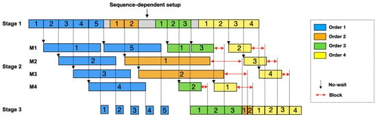
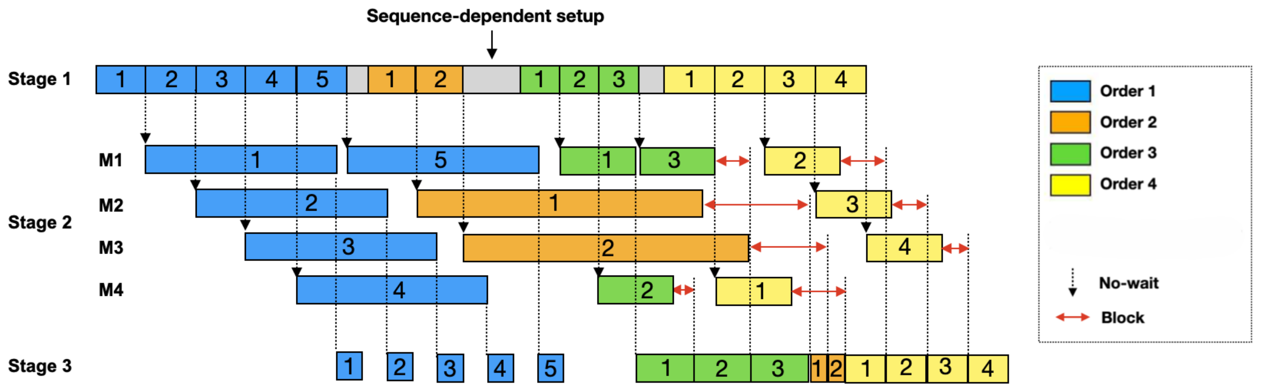
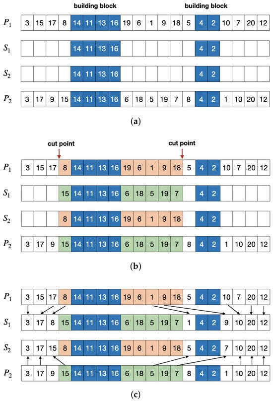
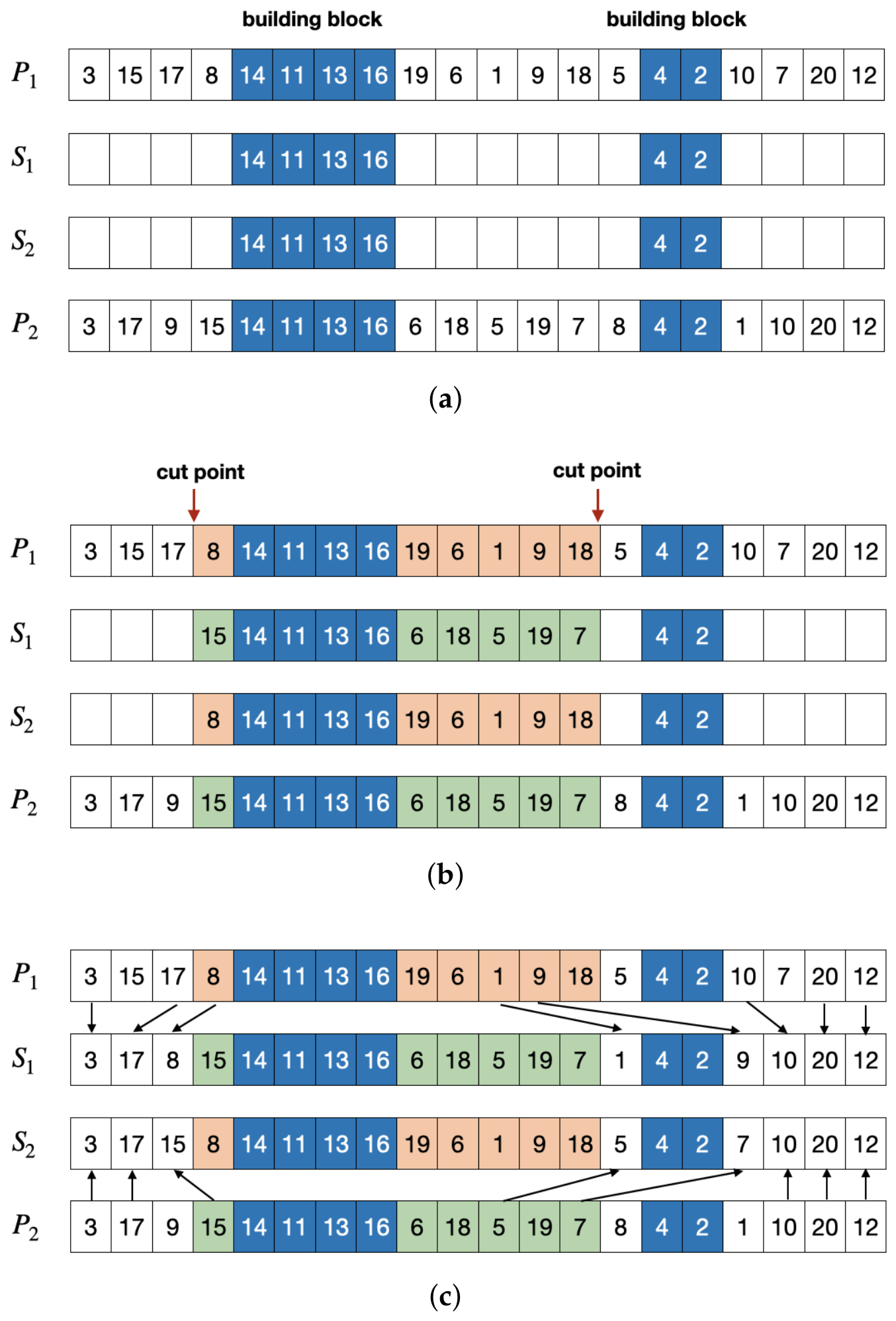
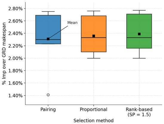
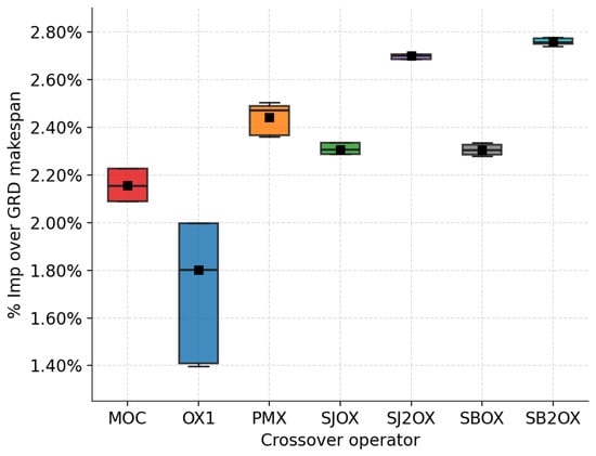
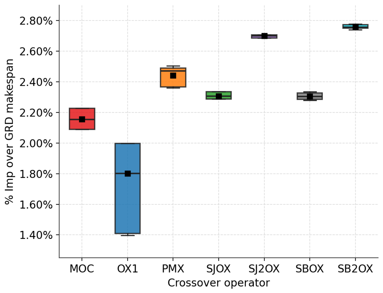
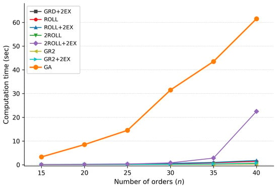
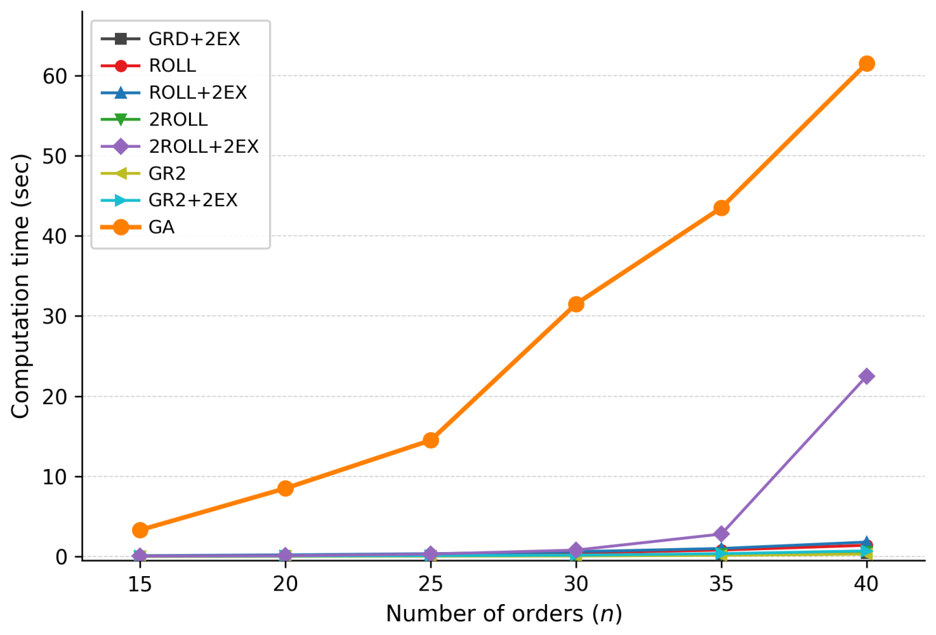
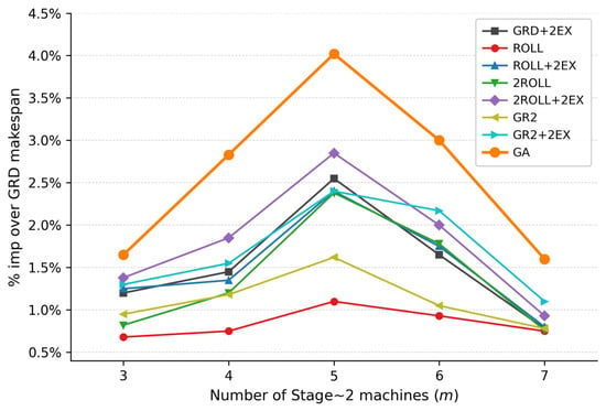
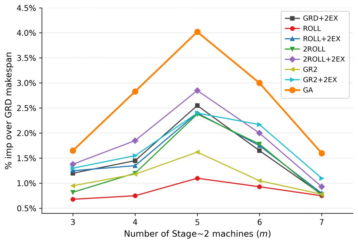
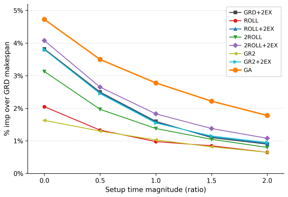
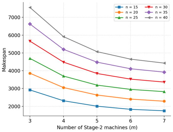
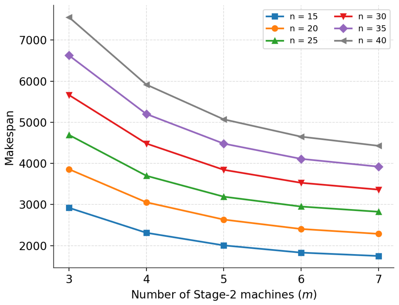
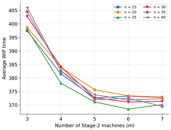
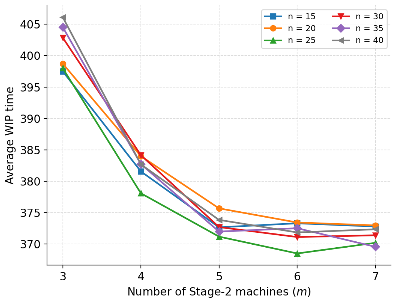
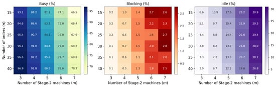
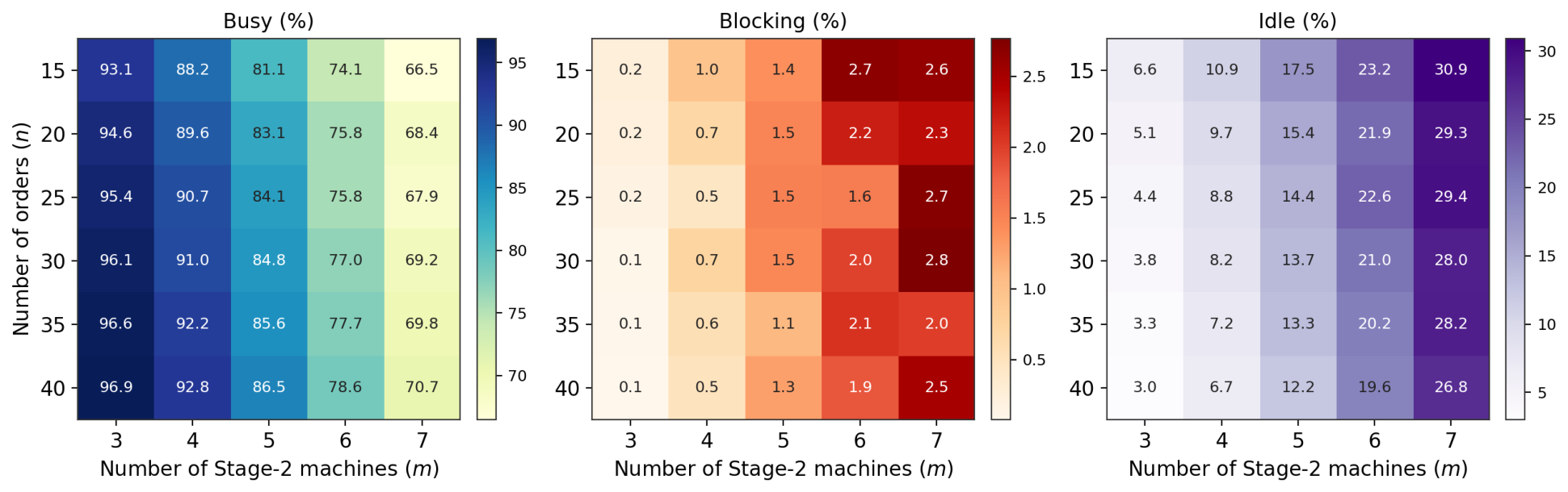

Disclaimer/Publisher’s Note: The statements, opinions and data contained in all publications are solely those of the individual author(s) and contributor(s) and not of MDPI and/or the editor(s). MDPI and/or the editor(s) disclaim responsibility for any injury to people or property resulting from any ideas, methods, instructions or products referred to in the content. |
© 2026 by the authors. Licensee MDPI, Basel, Switzerland. This article is an open access article distributed under the terms and conditions of the Creative Commons Attribution (CC BY) license.