


Highlights
Please indicate how your work links to systems science via your contributions to systems practice, theory, and/or methodology.
- We develop a dynamic shock-response measure of financial network resilience by integrating time-varying correlation networks with TVP-VAR impulse responses.
- The measure combines shock resistance and recovery duration to characterize resilience as an evolving property of the financial system.
What are the main findings and/or the implications of the main findings?
- Digital transformation exhibits an inverted U-shaped relationship with financial network resilience, with market trading activity and market illiquidity serving as key transmission channels.
- Economic policy uncertainty increases the curve’s concavity while partially mitigating the adverse marginal association at high digitalization levels, supporting adaptive risk monitoring and liquidity management.
Abstract
Digital transformation can strengthen financial systems by improving information processing and market efficiency, but it may also amplify interconnectedness and common exposures to shocks. This paper examines this trade-off by developing a dynamic shock-response framework for measuring financial network resilience and investigating its nonlinear relationship with digital transformation. Using daily adjusted closing prices of 95 listed Chinese financial institutions from 2008 to 2024, we construct dynamic financial correlation networks and characterize resilience along two dimensions, namely resistance to shocks and recoverability following shocks. These dimensions are quantified using impulse responses estimated from a TVP-VAR model. We then employ an RU-MIDAS framework to examine how digital transformation affects financial network resilience. The results show that network resistance declines markedly during major financial shocks, while recoverability deteriorates more substantially when multiple crises overlap. More importantly, digital transformation exhibits an inverted U-shaped relationship with financial network resilience, indicating that its resilience-enhancing effects diminish and eventually reverse beyond a certain level. Mechanism estimates reveal opposing indirect channels at the evaluated digital transformation levels. Declining trading activity is associated with weaker resilience, while reduced market illiquidity provides a positive compensating effect. Furthermore, economic policy uncertainty steepens this nonlinear relationship and partially mitigates the adverse effects at higher digitalization levels. These findings provide a dynamic perspective on financial network resilience and reveal the potential trade-off between the resilience benefits and systemic vulnerabilities associated with digital transformation.
1. Introduction
Digital transformation is fundamentally reshaping financial systems by improving information processing, transaction efficiency, and financial services [1]. At the same time, it is strengthening the interconnectedness of financial institutions and creating new channels for shock transmission across financial markets. While digital transformation can enhance financial stability by improving information processing and market efficiency, it may also amplify interconnectedness and common exposures to shocks, potentially undermining stability. Whether digital transformation ultimately strengthens financial network resilience or increases systemic vulnerability remains unclear. Addressing this issue is essential for understanding financial stability in the digital era.
Financial resilience has become an important perspective for understanding the stability of modern financial systems. It generally refers to the ability of financial markets or systems to withstand external shocks and recover from disruptions [2,3]. Existing studies commonly characterize resilience along two complementary dimensions: resistance, which captures the ability to absorb the initial impact of shocks, and recoverability, which reflects the speed at which the system returns to equilibrium after disturbances [4,5,6,7]. As financial institutions become increasingly interconnected, resilience should be understood not only as a property of individual institutions or markets but also as an attribute of the financial network formed by these interactions. Financial network resilience thus refers to the capacity of interconnected financial institutions to maintain core functions and restore stability following external shocks [8].
The literature on financial network resilience has expanded rapidly in recent years, examining the topic from several perspectives. One stream of research investigates how network structures influence systemic risk transmission and financial stability [9,10]. Another explores the resilience of financial networks under major crises and extreme events [11,12]. More recently, scholars have proposed strategies for improving network resilience by optimizing financial network structures and reducing contagion risks [13]. Despite these advances, the dynamic measurement of financial network resilience in response to external shocks remains insufficiently explored. Alternative approaches to constructing financial networks have distinct advantages and limitations. Correlation-based networks are easy to estimate and capture average co-movement, but they may miss tail dependence. Tail-risk networks focus on extreme downside risk but require relatively long samples and strong distributional assumptions. Variance-decomposition networks measure spillover intensity but do not directly map shock absorption and recovery. By contrast, the rolling-window FDR-filtered correlation network offers a transparent and flexible framework that captures time-varying interconnectedness while filtering out spurious weak links through FDR control, making it particularly suitable for tracking network evolution in rapidly changing financial environments. While this approach yields a linear representation, these features ensure computational tractability and interpretability.
To quantify financial resilience, the literature has mainly relied on three approaches: indicator-based methods, counterfactual estimation, and shock-response analysis. Indicator-based approaches construct composite resilience indices using selected economic or financial variables, whereas counterfactual methods evaluate resilience by comparing observed outcomes with hypothetical no-shock scenarios. Although widely adopted, both approaches rely heavily on indicator selection or model assumptions and are less capable of capturing the dynamic evolution of financial systems. By contrast, shock-response approaches based on impulse response analysis directly characterize how systems respond to and recover from external disturbances. In particular, the Time-Varying Parameter Vector Autoregression (TVP-VAR) model allows both parameters and shock transmission mechanisms to evolve over time, providing a more flexible framework for measuring resilience in rapidly changing financial environments [14,15,16].
Our resilience measure differs from existing connectedness and systemic-risk indicators in three respects. First, connectedness measures such as the Diebold–Yilmaz spillover index [17] capture the magnitude and direction of risk transmission, but they do not directly quantify how a network absorbs a shock or how quickly it recovers. Second, systemic-risk indicators that focus on the distress externalities or systemic importance of individual institutions, such as DebtRank [18], assess risk at the level of individual nodes, whereas our measure treats resilience as a dynamic property of the whole financial network. Third, by deriving resistance and recoverability from TVP-VAR impulse responses, our framework allows the shock-response mechanism itself to evolve over time. Thus, our measure complements rather than replaces existing connectedness and systemic-risk indicators.
The role of digital transformation in financial systems has also attracted growing scholarly attention. At the macro level, digital technologies have been shown to improve financial efficiency, information transparency, and risk monitoring capabilities [19,20,21]. At the micro level, digital transformation enhances firms’ operational efficiency, innovation, and financial resilience [22]. However, digitalization may also increase interconnectedness, technological dependence, and synchronization across financial institutions, thereby amplifying systemic risk contagion [23]. These contrasting effects suggest that digital transformation may exert both stabilizing and destabilizing influences on financial systems, implying a potentially nonlinear relationship with financial network resilience [24]. Nevertheless, empirical evidence on this issue remains limited, and the underlying transmission mechanisms have yet to be fully understood.
To address these research gaps, this study investigates the relationship between digital transformation and financial network resilience using China’s financial system as the empirical setting. First, we develop a dynamic framework for measuring financial network resilience from a shock-response perspective and quantify resilience in terms of resistance and recoverability based on impulse response functions estimated from a TVP-VAR model. Second, we employ the Reverse Unrestricted Mixed Data Sampling (RU-MIDAS) model to examine the nonlinear effect of digital transformation on financial network resilience and provide evidence of an inverted U-shaped relationship. Third, we identify the transmission mechanisms and boundary conditions underlying this nonlinear relationship by examining the mediating roles of market trading activity and market illiquidity and the moderating effect of economic policy uncertainty. China’s financial system, one of the world’s largest and most rapidly digitalizing, provides an appropriate setting for examining these issues. The findings contribute to the literature on financial network resilience by integrating dynamic resilience measurement with digital transformation and have useful implications for macroprudential regulation and digital financial governance.
2. Theoretical Analysis and Research Hypotheses
2.1. Digital Transformation and Financial Network Resilience
Digital transformation is fundamentally reshaping the operational logic and risk transmission pathways of the financial system. While enhancing information processing efficiency, optimizing risk management, and ensuring business continuity, digital technologies are also altering interconnections among financial institutions and risk transmission channels [25,26]. This implies that digital transformation does not uniformly strengthen or weaken financial network resilience; its impact depends on the relative strength of enabling effects and risk effects during digitalization.
At moderate levels of digital transformation, digital technologies can significantly enhance financial network resilience by improving information quality and strengthening risk response capabilities, with improvements in information transparency playing a critical role. Digital tools enable financial institutions to efficiently process vast amounts of operational and transactional data, using real-time data analysis to effectively alleviate information asymmetry [27] and curb irrational panic-driven trading behavior. Meanwhile, elastic computing systems ensure the continuity of critical operations under extreme external shocks [28], while distributed ledger technology enables precise identification and rapid isolation of risk nodes [29]. The combined effects of these mechanisms allow digital transformation to substantially strengthen both the resistance and recoverability of financial networks, thereby reinforcing overall financial network resilience.
However, excessive digitalization also creates new systemic risks, significantly undermining financial network resilience. As digitalization deepens, financial institutions gradually converge in their technological architectures, algorithmic trading models, and core data sources, exhibiting pronounced technological homogeneity [30]. Under normal conditions, homogeneous technological applications improve overall operational efficiency, yet under extreme market shocks, they can create severe hidden risks. Financial institutions, driven by similar algorithmic signals, simultaneously engage in risk-off selling and liquidity hoarding, causing localized and manageable risks to spread rapidly and evolve into system-wide risk resonance, thereby amplifying market volatility [31]. Meanwhile, heavy reliance on major third-party technology service providers creates concentrated infrastructure risks. If a core technology platform experiences a cyberattack or operational failure, it can paralyze the operations of multiple financial institutions simultaneously, leading to widespread financial service disruptions and significantly impairing the crisis recovery capacity of the financial network [32]. Moreover, the proliferation of high-frequency algorithmic trading further intensifies these risks [33]. Under market stress, homogeneous algorithms tend to trigger sell orders simultaneously, creating a self-reinforcing downward price spiral and markedly increasing the sensitivity of the financial network to external shocks. It follows that when digitalization reaches an excessively high level, systemic risks accumulate at an accelerating pace [34], exerting a pronounced negative impact on financial network resilience.
The interplay between these two mechanisms determines the net effect of digital transformation on financial network resilience. In the early stages of digital transformation, enabling effects such as reduced information asymmetry, enhanced risk identification capabilities, and improved business stability dominate, significantly strengthening financial network resilience as digitalization advances. When digital transformation surpasses a critical threshold, risk effects including technological homogeneity, infrastructure concentration, and algorithmic procyclicality gradually outweigh the benefits of digitalization. The marginal benefits of resilience enhancement continuously diminish and eventually become negative [35]. This pattern across stages indicates a significant inverted U-shaped relationship between digital transformation and financial network resilience. Accordingly, we propose the following research hypothesis:
H1.
Digital transformation exerts an inverted U-shaped effect on financial network resilience.
2.2. The Mediating Role of Market Trading Activity and Market Illiquidity
Market trading activity reflects the turnover frequency of financial assets and market participants’ willingness to trade, while market illiquidity measures transaction costs and market depth. Together, these two indicators characterize the overall quality of financial market functioning. Digital transformation can reshape the risk resistance and risk diffusion mechanisms of financial networks by altering market trading behavior and liquidity conditions. Therefore, market trading activity and market illiquidity serve as important transmission channels through which digital transformation affects financial network resilience [36].
Regarding market trading activity, the effects of digital transformation vary across stages. In the early stages of digital transformation, the proliferation of electronic trading platforms and algorithmic trading systems effectively reduces market transaction costs, enhances order execution efficiency, and broadens market participation, thereby significantly increasing market trading activity. Information-driven active trading enables financial institutions to rapidly adjust asset allocations and optimize risk hedging strategies under external shocks, thereby strengthening the risk resistance capacity of financial networks. However, as digitalization becomes excessive, algorithmic homogenization and stringent regulatory interventions may suppress speculative trading and reduce market turnover. This decline in trading activity impairs the price discovery process and weakens the market’s liquidity buffer. During periods of stress, the lack of active trading can trigger sudden liquidity spirals, exacerbating risk contagion and ultimately weakening financial network resilience [37,38]. In summary, digital transformation indirectly affects financial network resilience through phase-dependent changes in market trading activity.
Regarding market illiquidity, digital transformation also exhibits nonlinear effects [23]. In the early stages, digital transformation can temporarily increase market illiquidity due to structural friction, as capital rapidly reallocates toward digital-native assets, causing a temporary decline in market depth in traditional financial segments. However, as digitalization deepens and digital platforms mature, they broaden the investor base and significantly reduce information asymmetry, thereby decreasing market illiquidity [39]. Lower market illiquidity implies greater market depth and lower transaction costs, which helps financial institutions dispose of assets at reasonable prices when shocks occur, prevents price collapses and cascading default risks triggered by disorderly selling, and effectively maintains financial network stability. Conversely, high illiquidity amplifies the negative externalities of asset fire sales, causing localized idiosyncratic risks to spread through balance sheet interconnections and develop into systemic risks [40] and severely undermining financial network resilience [41]. Consequently, digital transformation indirectly affects financial network resilience through phase-dependent nonlinear changes in market illiquidity.
In summary, digital transformation affects financial network resilience through distinct channels. The turnover channel produces a negative transmission effect after its turning point, while the market illiquidity channel exhibits a compensating effect. Accordingly, we propose the following hypothesis:
H2.
Market trading activity and market illiquidity mediate the relationship between digital transformation and financial network resilience, with their indirect effects varying across digital transformation levels.
2.3. The Moderating Role of Economic Policy Uncertainty
Economic policy uncertainty reflects the degree of ambiguity in market participants’ expectations regarding fiscal, monetary, and regulatory policies [42]. It can significantly reshape financial institutions’ decision-making and the effectiveness of their digital transformation efforts, thereby creating substantial variation in how digital transformation affects financial network resilience [43].
At moderate levels of digitalization, the information processing advantages and low-cost trading benefits of digital technologies can effectively enhance financial network resilience [44,45], while high economic policy uncertainty further amplifies this positive enabling effect [46]. Under high economic policy uncertainty, market noise intensifies and policy signals become increasingly opaque, making it difficult for financial institutions to predict counterparty behavior and regulatory policy directions, thereby significantly increasing the risks associated with operational decisions [47]. In this context, the capabilities provided by digital transformation, such as precise information screening, multi-scenario risk simulation, and real-time risk warning, can deliver greater value, substantially increasing the marginal benefits of digital enablement and effectively helping financial institutions hedge against the adverse effects of policy uncertainty [48]. Therefore, high economic policy uncertainty reinforces the resilience-enhancing effect of moderate digitalization on financial networks.
When digitalization exceeds a critical threshold, issues such as technological homogenization, reliance on third-party infrastructure, and algorithmic procyclicality continuously undermine financial network resilience. While high economic policy uncertainty steepens the inverted U-shaped curve, it does not simply exacerbate the negative effects. On the one hand, policy ambiguity shortens financial institutions’ long-term planning horizons, making them more sensitive to market fluctuations. On the other hand, to hedge against policy and market risks, financial institutions may increasingly rely on advanced digital risk-control tools, such as real-time liquidity monitoring and multi-scenario stress testing. This defensive use of digitalization enhances risk identification and partially offsets the adverse effects of excessive digitalization [49]. Ultimately, while the curve becomes steeper, the ability to hedge risks through advanced digital tools partially mitigates the detrimental effects at higher digitalization levels [50].
In summary, economic policy uncertainty moderates the inverted U-shaped relationship by simultaneously amplifying the positive enabling effects at moderate levels and mitigating the adverse effects at excessive levels [51]. By increasing financial institutions’ sensitivity to both the enabling and risk effects, economic policy uncertainty moderates the inverted U-shaped relationship between digital transformation and financial network resilience, making the curve steeper. Accordingly, we propose the following hypothesis:
H3.
Economic policy uncertainty steepens the inverted U-shaped relationship between digital transformation and financial network resilience.
3. Methodology and Data
Financial network resilience [8] refers to the ability of the complex network formed by financial institutions and their interconnections to maintain core functions, resist shock propagation, and restore stability in the face of external shocks. To dynamically quantify financial network resilience, this study adopts a shock-response analytical framework and measures it along two dimensions, absorption intensity and recovery duration, using impulse response functions derived from the TVP-VAR model. Before measuring financial network resilience, two key tasks must be accomplished. The first is to construct a Financial Network Dynamic Index (FNDI) that captures the time-varying interconnected structure of the financial system. Specifically, we generate a dynamic correlation network using a rolling window and Pearson correlation coefficient matrices, and then employ principal component analysis (PCA) to extract an index that reflects the overall dynamics of the financial network from its topological and centrality characteristics. The second is to delineate the response path of the financial network to external shocks and measure its response characteristics, a process that can be effectively captured by the impulse response functions of the TVP-VAR model. Accordingly, the construction of our financial network resilience measurement model consists of the following four components.
3.1. Data Sources
The sample spans 2008 to 2024. We construct the financial network based on the adjusted closing price data of 95 listed Chinese financial institutions to measure financial network resilience. The sample comprises 42 banks, 47 securities firms, and 6 insurance companies. Since some institutions were listed after the start of our sample period, the sample composition varies across years. All stock price data are obtained from the Tushare database. In addition, we select the S&P 500 Volatility Index (VIX) as the external shock variable. This index is widely regarded as the fear gauge of global financial markets and effectively captures changes in international risk sentiment. A rise in the VIX signals stronger global risk aversion, weaker risk appetite among global investors, and capital flight from emerging to developed economies. These trends put downward pressure on China’s financial market stability. Meanwhile, a rising VIX is associated with heightened global economic uncertainty, which transmits to China’s real economy through trade linkages, affecting corporate profitability and solvency, and thereby indirectly influencing financial network resilience. Although the impact of the VIX on China’s financial system is indirect, it is strongly exogenous, as it primarily reflects U.S. market sentiment and is largely unaffected by internal factors within China’s financial system. Therefore, it is appropriate to use the VIX as a proxy for external risk shocks. The construction of the financial network, FDR control, PCA, and the TVP-VAR estimation were performed in R (version 4.5.0; R Foundation for Statistical Computing, Vienna, Austria).
3.2. Measurement of Financial Network Resilience Characteristics
3.2.1. Financial Network Construction
To capture the dynamic linkages among financial institutions, we employ the rolling correlation threshold method [52] to construct a time-varying financial network and extract its topological and centrality characteristics. This approach uses a rolling window to capture the time-varying interconnectedness of the financial system and uses false discovery rate (FDR) control to retain only statistically significant correlations, ensuring the robustness of the network structure [53]. The construction proceeds as follows.
We first convert the daily closing prices of listed Chinese financial institutions into log returns:
where is the log return of stock i at time t, and is the closing price of stock i at time t. Next, we set a rolling window of length L with step size s, which partitions the return series into overlapping sub-periods. Within each window, we compute Pearson correlation coefficients between all institution pairs, generating a time-varying correlation matrix :
To identify statistically significant correlations, we apply the FDR approach [54]. With a significance level , we determine the adjusted threshold such that , where is the total number of possible institution pairs. We then construct the weighted adjacency matrix as follows:
where represents the absolute value of the Pearson correlation coefficient, serving as the edge weight between nodes and . To calculate the weighted shortest paths, we transform the edge weights into distances using . This yields a time-varying adjacency matrix that captures the evolving network structure. Based on , we obtain the topological and node centrality indicators of the financial network, as summarized in Table 1. These indicators collectively characterize the structural fragility, risk transmission paths, and systemic risk evolution of the financial system.
Table 1.
Network characteristic indicators.
3.2.2. Construction of FNDI
Network topology indicators reveal the macro-environment and potential scope of risk contagion [17,53], while centrality indicators identify systemically important nodes in the network [18]. The joint dynamics of these two types of indicators characterize the evolution of the financial system’s risk state [55,56]. To synthesize these network indicators into a comprehensive index that captures the overall state of the financial network, this study employs PCA to construct FNDI. This method effectively extracts the information on systemic risk shared across multiple network indicators, mitigating the information bias inherent in any single indicator. In addition, PCA addresses multicollinearity among indicators through orthogonal transformation, enhancing the statistical reliability and stability of the resulting index. Moreover, as PCA determines weights based on the variance structure of the data, it reduces the influence of subjective judgment and provides a robust, comprehensive quantitative measure of the overall state of the financial network.
The principal components are obtained as linear combinations of the standardized indicators:
where are the standardized indicators and are the component loadings. The FNDI is then constructed as the weighted sum of the first k principal components, with weights proportional to their variance contribution rates.
3.2.3. Time-Varying Parameter Vector Autoregression (TVP-VAR) Model
The TVP-VAR model, with time-varying parameters [14,57], captures the dynamic and evolving relationships among variables in the economic system. The model is specified as:
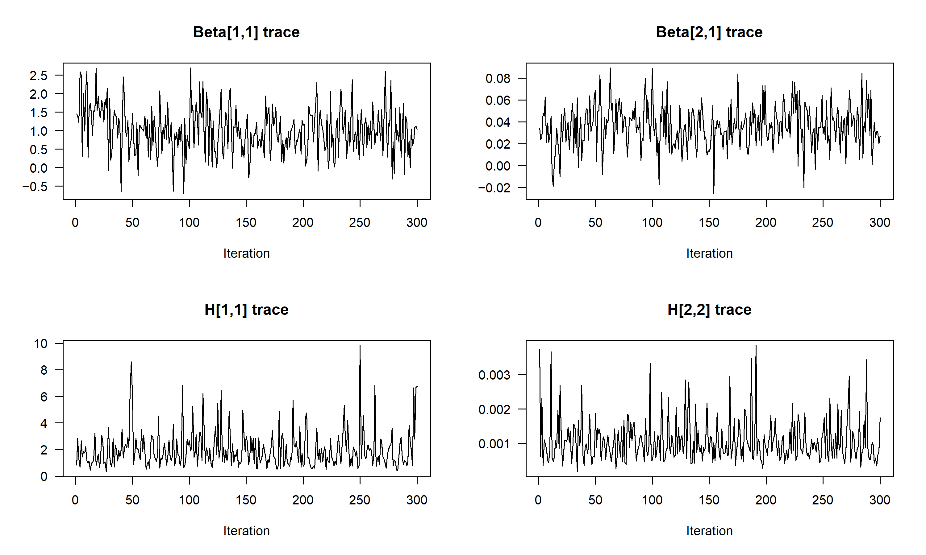
where is ordered as . This VIX-first Cholesky ordering implies that VIX affects FNDI contemporaneously, while FNDI affects VIX only with a lag, reflecting the exogeneity of global risk sentiment to China’s financial network; (for ) are matrices of time-varying coefficients; is a lower-triangular matrix; is a diagonal matrix with ; and is the error term. In this paper, we employ the Bayesian MCMC method to estimate the TVP-VAR model, with 3000 iterations and 1000 burn-in, using default priors. Detailed settings, including lag selection, identification, and convergence diagnostics, are provided in the Appendix A.
3.2.4. Quantification of Network Resilience via Impulse Responses
Following Chen et al. [58], we employ VIX as the external shock variable and estimate a TVP-VAR model including both VIX and FNDI to derive the impulse response function () of FNDI to VIX shocks. Based on this function, we construct two resilience measures, absorption intensity () and recovery duration (), as follows:
where t denotes the specific calendar time when the shock occurs, and i denotes the i-th response period after the shock. The absolute value of is used to capture the overall impact of shocks on the financial network, as the impulse response may take negative values. N denotes the number of periods required for the impulse response function to converge to zero. In addition, following Hamilton [59], we employ a Markov-switching (MS) model to identify low-resilience regimes by detecting the durations during which an absorption intensity is in its low state and recovery duration is in its high state.
4. Measurement Results and Analysis of Financial Network Resilience
4.1. Descriptive Analysis of Financial Network Characteristics
To balance estimation stability and time-varying dynamics, we adopt a rolling window of 120 trading days with a step size of one day to measure the dynamic changes in the topological and centrality characteristics of the financial network. The annual means of the resulting financial network characteristics are presented in Table 2.
Table 2.
Annual means of financial network characteristics.
Table 2 shows that the interconnected network of Chinese financial institutions is characterized by relatively short path lengths and high clustering coefficients. PL is calculated using weighted shortest paths, where the edge distance is defined inversely to the correlation strength. Thus, in years with highly synchronized movements, strong correlations result in shorter weighted paths, indicating highly efficient information transmission. Conversely, in years with a sparser network, the paths become longer due to structural fragmentation. The ND remains at a high level for most of the sample period, fluctuating between 0.705 and 1.000. It reaches its maximum of 1.000 during the 2008 financial crisis, drops to a trough of 0.705 in 2017, rebounds to 0.998 during the 2020 pandemic, and then declines to 0.822 in 2024. The CE follows a similar pattern, gradually declining from 0.878 in 2008 to 0.795 in 2024, with a notable trough of 0.711 in 2017. These patterns suggest that although a few highly connected core institutions exist in the network, their systemic importance has gradually decreased over time.
4.2. Empirical Extraction of FNDI
We employ PCA to reduce the dimensionality of the network characteristic indicators and construct FNDI, a composite measure that captures the overall dynamics of the financial network. Before performing PCA, Bartlett’s test of sphericity is conducted on the indicators. As shown in Table 3, the KMO value is 0.60 and the p-value is less than 0.01, indicating that the selected indicators are suitable for PCA.
Table 3.
Bartlett’s test of sphericity.
The explained variance is presented in Table 4. The first principal component has an eigenvalue greater than 1, with a cumulative variance contribution rate of 63.184%. This indicates that the first principal component effectively captures the overall dynamic characteristics of the financial network while retaining sufficient information. Therefore, the FNDI is constructed from this first principal component, and the composite score coefficients of each indicator are presented in Table 5.
Table 4.
Total variance explained.
Table 5.
Composite score coefficient matrix.
4.3. Trends of FNDI and VIX
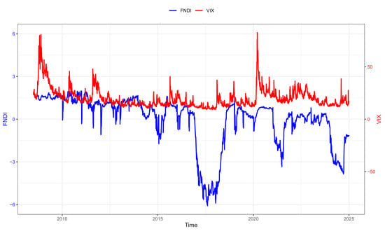
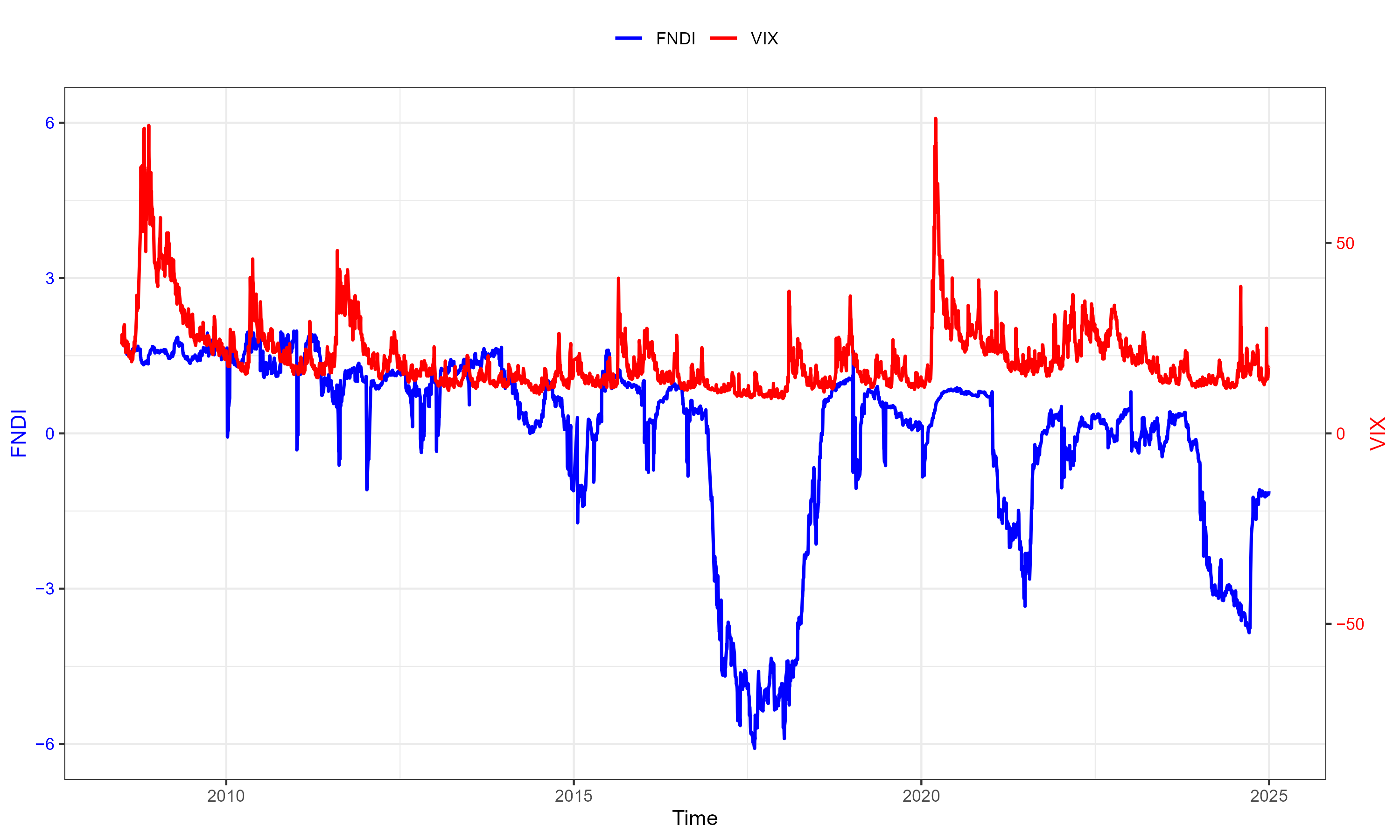
In Figure 1, the red line represents VIX, reflecting China’s external financial risk conditions, while the blue line represents FNDI, capturing the dynamic evolution of China’s financial network. The fluctuations of FNDI and VIX exhibit synchronized movements, as seen during the 2008 financial crisis and the 2020 COVID-19 pandemic, when both indices experienced notable volatility. The correlation coefficient between the two series is 0.3436. Moreover, although FNDI is positively correlated with VIX, the calculation of the resilience characteristics (absorption intensity and recovery duration) depends solely on the dynamic area of impulse response functions under external risk shocks (Equations (6) and (7)), and is independent of the sign of the correlation coefficient. Therefore, FNDI is suitable for the modeling analysis in this paper.
Figure 1.
Trends of FNDI and VIX.
4.4. Impulse Response Function of FNDI to VIX
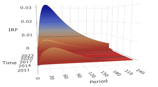
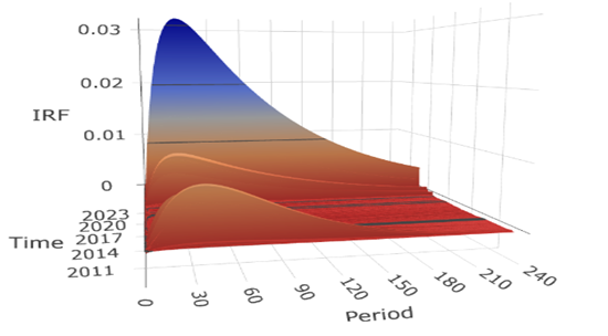
Figure 2 presents a three-dimensional impulse response plot based on the TVP-VAR model, which reflects the impact of external risk shocks on China’s financial network. The X-axis represents the response horizon, the Y-axis represents the timing of VIX shocks, and the Z-axis represents the impulse response values of FNDI to VIX shocks. The results show that the response of FNDI to VIX shocks is predominantly positive over the sample period, with values ranging from 0 to 0.031.
Figure 2.
Impulse response function of FNDI to VIX.
In terms of the response horizon, the impact reaches its peak at around 30 days and then converges slowly, approaching zero over approximately 240 trading days (about one year). This slow convergence reflects the long-memory nature of daily data. Over calendar time, the strongest response occurs around 2020, coinciding with the COVID-19 outbreak when the VIX surged to historically high levels. A moderate response is also observed during 2008–2012, corresponding to the global financial crisis and the subsequent European sovereign debt crisis. During 2012–2017, the response remains relatively muted, consistent with a period of comparative market stability. Overall, the results suggest that external risk shocks lead to a deterioration in financial network resilience, with the magnitude of this effect being time-varying and particularly pronounced during periods of extreme market turbulence.
4.5. Resilience Characteristics of China’s Financial Network
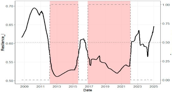
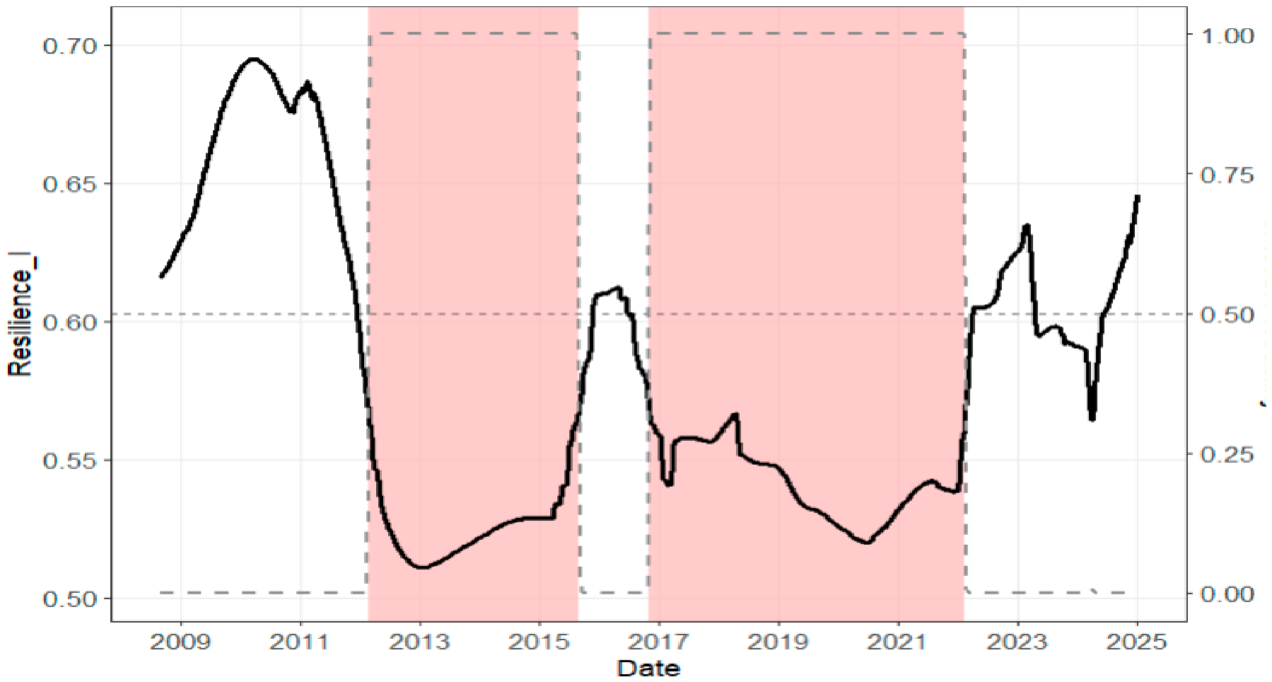
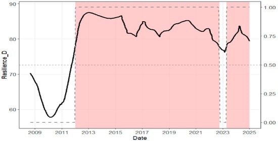
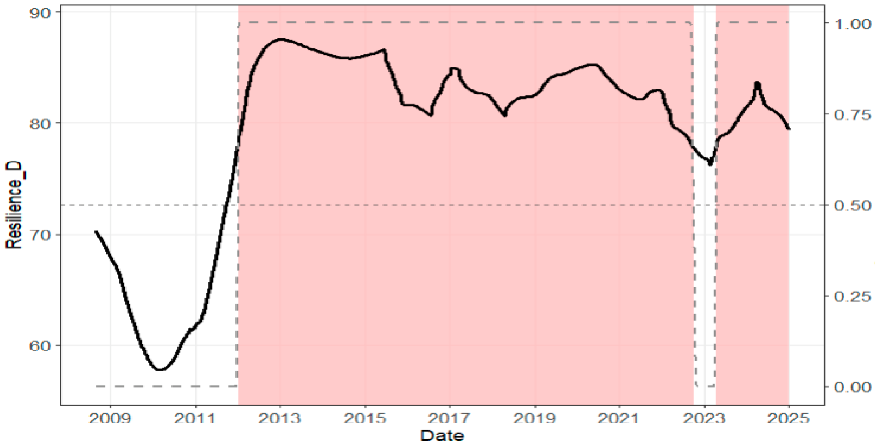
Figure 3 and Figure 4 present the dynamic evolution of the two resilience characteristics in China’s financial network, resistance and recoverability. Resistance is captured by absorption intensity, while recoverability is captured by recovery duration. Low absorption intensity indicates a state of weak resistance, whereas a long recovery duration indicates a state of slow recovery, both of which point to lower levels of financial network resilience. The dashed lines represent the smoothed probabilities estimated from the MS model, and the red shaded areas identify the periods classified as low-resilience regimes.
Figure 3.
Resistance and smoothed probability of the low state.
Figure 4.
Recoverability and smoothed probability of the low state.
The figures show that the resilience characteristics of China’s financial network alternate between high and low states, exhibiting asymmetric and phase-specific fluctuations. Notably, while both resistance and recoverability identify two distinct low-resilience episodes, their temporal patterns differ substantially. This divergence reflects the distinct nature of the two dimensions: resistance captures instantaneous shock absorption and is more responsive to transient disturbances, whereas recoverability reflects the speed of adjustment following structural disruptions and is therefore highly persistent once impaired.
To identify these low- and high-state episodes, this paper adopts the MS model following Hamilton [59]. The low-resilience periods are determined by the intersection of the estimated smoothed probabilities with the 0.5 threshold, in conjunction with the trajectory of the resilience characteristic curves. The specific phases are presented in Table 6. For resistance, the first phase (2012–2015) corresponds to the aftermath of the European sovereign debt crisis and the 2015 stock market crash. The second phase (2016–2022) reflects the compounded effects of domestic financial deleveraging, US–China trade frictions, and the COVID-19 pandemic. In stark contrast, for recoverability, the first low-state phase spans a decade (2012–2022), indicating a strong hysteresis effect: even when the network’s resistance temporarily recovered, its recovery speed remained structurally sluggish due to successive overlapping shocks. The second low-recoverability phase (2023–2024) reflects ongoing challenges posed by the real estate liquidity crisis, geopolitical conflicts, and external monetary tightening, which prolonged the recovery time of China’s financial network.
Table 6.
Low-resilience periods of China’s financial network.
4.6. Robustness Test of Resilience Characteristics Measurement
As reported in Table 7, we recalculate the FNDI with window lengths of 100, 110, 120, and 130 trading days, and compute their correlations with the benchmark FNDI. All correlation coefficients exceed 0.979, indicating that the FNDI series are highly consistent and that the window length does not materially affect the construction of the FNDI.
Table 7.
Sensitivity analysis of window length.
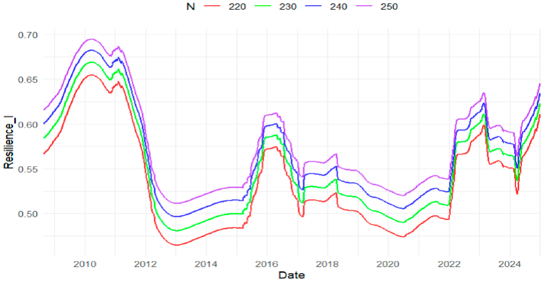
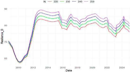
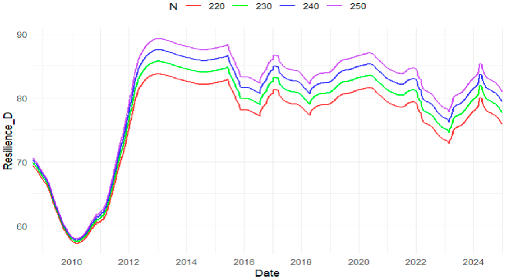
We conduct a robustness check by setting the impulse response convergence horizon N to 220, 230, 240, and 250 to examine the impact of different convergence horizons on the measurement results. As shown in Figure 5 and Figure 6, the resilience characteristic curves under these convergence horizons exhibit highly consistent dynamic trajectories, indicating that the financial network resilience measurements in this paper are robust to the choice of N. Furthermore, a correlation analysis is conducted to examine the relationships among resilience characteristics under different convergence horizons, and the results are presented in Table 8. The correlation coefficients all exceed 0.99, which further supports the reliability of the resilience characteristic measurements.
Figure 5.
Robustness analysis of resistance.
Figure 6.
Robustness analysis of recoverability.
Table 8.
Correlation coefficients.
5. Empirical Analysis of the Effects of Digital Transformation
5.1. Variable Definitions
- (1)
- Dependent Variable
We employ the entropy weight method to construct a composite index of financial network resilience (FNR) based on the two resilience characteristics derived from the above analysis, resistance and recoverability. The index construction is presented in Table 9.
Table 9.
Construction of FNR.
- (2)
- Explanatory Variable
The explanatory variable is digital transformation (DIG), sourced from CSMAR. It is derived from a weighted score across six dimensions for listed firms. To capture the overall transformation trend of the financial industry, we select all listed firms in the financial sector, compute the arithmetic mean of their annual digital transformation indices, and construct the annual average digital transformation index for the financial industry. Since the raw data span the period 2011–2024, we first employ linear extrapolation to estimate the missing values for 2008–2010. To address the frequency mismatch and avoid pseudo-replication, we further apply the Chow-Lin method to disaggregate the annual DIG into a monthly series. The high-frequency indicators used for disaggregation, namely mobile phone users, fixed broadband subscribers, and telecom business revenue, are sourced from the Ministry of Industry and Information Technology (MIIT). All series are processed into monthly values to ensure frequency alignment, and the Chow-Lin procedure is estimated using the maximum likelihood method. The consistency check confirms that the annual mean of the disaggregated monthly DIG matches the original annual DIG exactly for all years.
- (3)
- Control Variables
We select the year-on-year growth rate of the end-of-period balance of money and quasi-money (M2), the CPI year-on-year growth rate (CPI), the national manufacturing PMI (PMI), and the consumer confidence index (CCI) as control variables to ensure the robustness of the empirical results. M2 captures the overall liquidity conditions of the economy; CPI reflects changes in domestic purchasing power; PMI (with 50 as the threshold) serves as a proxy for expectations regarding macroeconomic activity; and CCI captures the confidence and expectations of microeconomic agents. Data are sourced from the People’s Bank of China and the National Bureau of Statistics.
- (4)
- Mediating Variables
We employ market turnover (Turnover) and the Amihud illiquidity measure (AILLIQ) as proxy variables for market trading activity and market illiquidity, respectively. Turnover reflects the degree of trading activity, with higher turnover indicating a greater willingness among investors to trade and faster incorporation of information into prices. AILLIQ captures the price impact per unit of trading volume; lower values indicate greater market depth and lower transaction costs, corresponding to a lower level of market illiquidity. All data are sourced from the CSMAR database.
- (5)
- Moderating Variable
The Economic Policy Uncertainty Index of China (EPU) is used as the moderating variable. It is sourced from the CSMAR database and compiled from reports from the People’s Daily and Guangming Daily, reflecting the degree of uncertainty in the macroeconomic environment in mainland China. To reduce skewness and mitigate potential multicollinearity, the EPU index is logarithmically transformed and then mean-centered.
5.2. Model Construction for the Effects of Digital Transformation
To address the frequency mismatch among variables, this study employs the RU-MIDAS model proposed in [60], which extends monthly low-frequency variables to the daily frequency by assigning the same value to all daily observations within a given month. This specification is equivalent to a mixed-frequency data model under equal-weighting constraints [61]. Because the monthly-frequency regressors are constant within each calendar month, the residuals may exhibit serial correlation within the same month. Accordingly, the baseline model incorporates month-of-year and day-of-the-week fixed effects to control for seasonal and cyclical fluctuations. Standard errors are clustered at the year-month level for statistical inference. The baseline model is specified as follows.
We specify the following baseline regression model to test H1. The explanatory variable, digital transformation (), is measured at the monthly frequency and is extended to daily data by assigning the same value to all daily observations within a given month, i.e., .
where denotes the financial network resilience on day t; is the level of digital transformation, and is its squared term; are control variables, all of which are monthly data and are also extended to the daily frequency; , denote month and day-of-the-week fixed effects, respectively; and is the idiosyncratic error term.
We specify the following mediation model to test H2. We employ Turnover and AILLIQ as mediating variables to examine the transmission mechanisms through which digital transformation affects financial network resilience, focusing on market activity and market liquidity.
where represents the mediating variable on day , which is proxied by Turnover and AILLIQ, respectively. Equation (9) tests the nonlinear effect of digital transformation on the mediator, while Equation (10) augments the baseline model with the mediator to examine its mediating effect.
The moderating effect model is formulated as follows to test H3. We employ the Economic Policy Uncertainty Index of China () as a moderating variable. This index is originally at a monthly frequency and is converted to daily frequency (), with all trading days within the same month sharing the same value.
where is the interaction term between the linear term of digital transformation and the moderator, and is the interaction term between the quadratic term of digital transformation and the moderator.
5.3. Empirical Results and Analysis
5.3.1. Baseline Regression Analysis
The results of the baseline regression model are presented in Table 10. Column (1) presents the specification without control variables, while Column (2) adds the full set of control variables. In both specifications, the estimated coefficient of the linear term of DIG is significantly positive, and that of the squared term is significantly negative. From column (2), the estimated coefficient of DIG is 8.637, and that of is 1.389, both of which are statistically significant at the 1% level. This indicates an inverted U-shaped relationship between digital transformation and financial network resilience, thus confirming H1.
Table 10.
Baseline regression results.
We further verify the robustness of the inverted U-shaped relationship between digital transformation and financial network resilience using the Utest procedure proposed by Lind & Mehlum [62]. The test results are presented in Table 11. The slope at the lower bound of the interval is significantly positive (1.613, p < 0.01), while the slope at the upper bound is significantly negative (−2.154, p < 0.01), satisfying the necessary conditions for the existence of an inverted U-shaped relationship. The turning point is 3.11, which lies within the actual range of the digital transformation variable [2.529, 3.886]. The overall p-value is 1.45 × 10⁻⁷, leading to rejection of the null hypothesis at the 1% significance level. This confirms the existence of an inverted U-shaped relationship between digital transformation and financial network resilience and the robustness of the baseline regression results.
Table 11.
Utest results.
5.3.2. Robustness Tests
- (1)
- Monthly aggregated regression.
To examine whether the findings are sensitive to the repetition of monthly regressors across daily observations, we aggregate the daily variables to the monthly frequency, yielding a sample of 197 monthly observations. We then re-estimate the baseline model using robust standard errors and month fixed effects. As shown in Column (1) of Table 12, the coefficients for DIG (8.507) and DIG2 (−1.368) remain significantly positive and negative, respectively, at the 1% level. This cleaner test confirms that our inverted U-shaped findings are not driven by repeated daily observations and are highly robust.
Table 12.
Robustness Tests results.
- (2)
- Excluding the extrapolated period
To address the concern about the extrapolated period, we re-estimate the baseline regression by excluding the years 2008–2010. As shown in Column (2) of Table 12, Robustness Tests results, the coefficients of DIG and are 4.692 and −0.754, respectively, both significant at the 1% level. The inverted U-shaped relationship remains robust, confirming that our core conclusion is not driven by the extrapolated period.
- (3)
- Quantile regression
The robustness of the inverted U-shaped relationship across different resilience levels is further examined using quantile regressions at the 0.25, 0.5, and 0.75 quantiles. As shown in Column (3) of Table 12, the coefficient of the linear term is significantly positive and that of the squared term is significantly negative across all quantiles, confirming that the inverted U-shaped relationship between digital transformation and financial network resilience remains robust regardless of the resilience level.
- (4)
- Alternative measures of the dependent variable
To further verify the robustness of our results, we replace the dependent variable with its two sub-dimensions: resistance and recoverability. As shown in the last two columns of Table 12, the coefficients of the linear and squared terms of DIG on resistance are 1.616 and −0.259, respectively, both significant at the 1% level, indicating an inverted U-shaped relationship. For recoverability (measured by recovery duration, where a longer duration indicates lower recoverability), the coefficients are −3.426 and 0.551, respectively, both significant at the 1% level, indicating a U-shaped relationship. This indicates that digitalization initially shortens the recovery duration (enhancing recoverability) but prolongs it at higher levels (weakening recoverability). Notably, the implied turning points for resistance and recoverability (approximately 3.12 and 3.11) both fall well within the valid DIG sample range [2.529, 3.886]. These results consistently confirm that the inverted U-shaped relationship holds across different dimensions of financial network resilience.
5.3.3. Endogeneity Tests
Although the baseline results remain robust to the checks reported above, potential endogeneity between digital transformation and financial network resilience may still be a concern. We therefore conduct the following additional analyses.
- (1)
- Lagged-term test. We further assess the robustness of the nonlinear relationship by re-estimating the model using the one-period lag of digital transformation and its squared term as explanatory variables. As shown in Column (1) of Table 13, the coefficient of the lagged linear term is significantly positive (8.860, p < 0.01), while that of the squared term is significantly negative (−1.425, p < 0.01), consistent with the sign pattern of the baseline regression. These results indicate that the nonlinear relationship remains robust when lagged DIG is used, although this specification does not provide causal identification.Table 13. Endogeneity test results.
- (2)
- Excluding extreme years. Considering that the 2008 global financial crisis and the 2020 COVID-19 pandemic may have exerted extreme shocks on financial network resilience, we exclude these two years from the sample and re-estimate the model. As shown in Column (2) of Table 13, the coefficient of the linear term of digital transformation is significantly positive (7.549, p < 0.01), while that of the squared term is significantly negative (−1.219, p < 0.01). The inverted U-shaped relationship remains robust, indicating that our core conclusion is not driven by extreme years.
5.3.4. Mediating Effect Analysis
The mediation analysis results are presented in Table 14. In Column (1), the coefficients of the linear and squared terms of digital transformation on Turnover are 5.291 and −0.860, respectively, and are significant at the 10% and 5% levels, yielding a turning point of approximately 3.076. In Column (3), the coefficients on AILLIQ are 1.306 and −0.207, respectively, both significant at the 1% level, with a turning point of approximately 3.155. In Columns (2) and (4), the coefficients of Turnover (0.069, significant at the 5% level) and AILLIQ (−0.713, significant at the 1% level) indicate their opposing marginal associations with network resilience. Overall, these results support H2, confirming that market trading activity and market illiquidity mediate the relationship between digital transformation and financial network resilience, with their indirect effects varying across digitalization levels and exerting distinct influences.
Table 14.
Mediating effect results.
To further verify the nonlinear mediating channels, we employ a bootstrap method. The results are reported in Table 15. The evaluated DIG percentiles (3.58, 3.69, and 3.74) are located in the high-digitalization regime, exceeding the calculated turning points of both mediators (3.076 for Turnover and 3.155 for AILLIQ). At these high-digitalization levels, the AILLIQ channel exhibits a significantly positive indirect effect, with all bias-corrected 95% confidence intervals excluding zero. This indicates that the continuous reduction in market illiquidity serves as a positive compensating channel for resilience. Conversely, the Turnover channel exhibits a negative indirect effect. Its bias-corrected confidence intervals also exclude zero, while its associated p-values range from 0.083 to 0.095, indicating that this negative mediating effect is only marginally significant (at the 10% level). This suggests that the suppression of trading activity in the highly digitalized setting reduces market liquidity buffers, thereby weakening the positive contribution of active trading to network resilience and resulting in a net negative mediation effect for the turnover channel. Overall, these findings provide robust evidence for H2, confirming that market trading activity and market illiquidity mediate the relationship between digital transformation and financial network resilience, with their indirect effects varying across digitalization levels.
Table 15.
Bootstrap test results for nonlinear mediating effects.
5.3.5. Moderating Effect Analysis
We examine the moderating effect of EPU by sequentially adding the linear and quadratic interaction terms between digital transformation and EPU to the baseline model. The results are presented in Table 16. In both models, the coefficient of the linear term of DIG is significantly positive, while that of the squared term is significantly negative, suggesting that the inverted U-shaped relationship remains robust across different specifications. In Column (2), the coefficient of is −0.054 and significantly negative at the 1% level, indicating that the inverted U-shaped curve becomes more concave as EPU increases.
Table 16.
Moderating effect results.
To clarify this moderating effect, we evaluate the cross-partial derivative of the marginal effect: . Within the observed DIG sample range [2.529, 3.886], this expression remains strictly positive. This implies an upward shift in the marginal association between DIG and resilience as EPU increases, thereby mitigating the adverse effects at higher DIG levels. The conditional turning points calculated across the EPU range also fall within the valid DIG sample bounds. Therefore, these estimates support the moderating role of EPU through simultaneous changes in curvature and slope. Thus, H3 is verified.
5.3.6. Heterogeneity Analysis
- (1)
- Temporal heterogeneity
Given differences in policy environments and market conditions across periods, the impact of digital transformation on financial network resilience may exhibit heterogeneity. To this end, we conduct a temporal heterogeneity analysis. In 2015, the Chinese State Council’s “Government Work Report” first proposed the “Internet+” action plan, marking the launch of China’s digital transformation strategy. Using this as the cutoff, we divide the sample into two sub-periods, 2008–2015 and 2016–2024, and perform group-wise regressions to compare the effects before and after the policy shift.
The group-wise regression results are presented in Table 17. Both sub-periods exhibit a significant inverted U-shaped relationship. In the 2008–2015 period, the coefficient of the linear term of digital transformation is 6.623, while that of the squared term is −1.061. In the 2016–2024 period, the coefficient of the linear term is 1.019, and that of the squared term is −0.161. Descriptively, the absolute magnitude of the linear coefficient is larger in the earlier period (6.623 vs. 1.019), suggesting a steeper initial slope. By comparison, the marginal effect tends to weaken and the curve becomes flatter in the later period. This may be attributed to the fact that digital transformation has become increasingly pervasive in recent years, and the financial industry has gradually moved beyond the phase of rapid marginal improvement.
Table 17.
Heterogeneity results.
- (2)
- Heterogeneity across market volatility regimes
We examine the heterogeneous effects of digital transformation on financial network resilience under different market volatility conditions by dividing the sample into high-volatility and low-volatility periods based on the historical median of the VIX index and performing separate regressions for each regime. The results are presented in Table 17. The inverted U-shaped relationship between digital transformation and financial network resilience remains significant under both volatility regimes. A comparison of the coefficient estimates across the two groups reveals that, in the low-volatility period, the coefficient of the linear term of digital transformation is 10.772, which is larger than 8.315 in the high-volatility period, and the absolute value of the squared term coefficient is also larger. Based on the coefficient magnitudes, the inverted U-shaped curve appears steeper in the low-volatility regime. This difference may be explained by the fact that, in relatively stable market environments, financial institutions have more resources to undertake substantive digital transformation, allowing digital investments to translate more effectively into improvements in operational efficiency and risk prevention capabilities. In contrast, during high-volatility periods, financial institutions face liquidity pressures and heightened risk-aversion motives, making it more difficult to fully realize the potential benefits of digital investments, resulting in a flatter inverted U-shaped curve.
6. Conclusions
Using daily closing price data for financial institutions from 2008 to 2024, we construct a dynamic financial network and employ the TVP-VAR model to measure financial network resilience. We further apply an RU-MIDAS model to examine empirically the impact of digital transformation on financial network resilience and its underlying mechanisms. The measurement results show that the resilience characteristics of China’s financial network alternate between high and low states, with varying durations across different phases. On this basis, we examine the impact of digital transformation on financial network resilience and draw the following main conclusions: (1) digital transformation has an inverted U-shaped effect on financial network resilience; (2) market trading activity and market illiquidity are key mediating channels, with the trading-activity channel exerting a negative effect and the illiquidity channel providing a positive compensating effect across the evaluated digitalization levels; and (3) economic policy uncertainty significantly moderates this relationship by steepening the inverted U-shaped curve and shifting the marginal association upward at higher digitalization levels.
These findings have several policy implications. First, financial institutions should pursue digital transformation prudently, balancing the benefits of technological advancement against potential risks such as technological homogenization and over-reliance on third-party service providers. Regulatory authorities should establish dynamic monitoring mechanisms to guide the healthy development of digital transformation in the financial sector. Second, attention should be paid to changes in market trading activity and market illiquidity. Financial institutions should use digital transformation to enhance information transparency and trading efficiency, promote reasonable trading activity, alleviate market illiquidity, and strengthen the resilience of the financial system. Regulators should monitor abnormal fluctuations in market turnover and liquidity dry-ups to prevent excessive speculation and market dysfunction. Third, the impact of economic policy uncertainty should be taken seriously, and differentiated regulatory approaches should be implemented. During periods of high economic policy uncertainty, digital transformation has a more pronounced effect on financial network resilience. Regulators should strengthen policy communication and expectation guidance to reduce the interference of policy uncertainty on financial institutions’ decision-making, while also enhancing the monitoring and early warning of digital transformation risks during such periods.
7. Limitation
Despite its contributions, this study has several limitations. First, monthly DIG is estimated using the Chow-Lin disaggregation method. Although the annual mean of the disaggregated series perfectly matches the original annual DIG, the within-year variation is model-based rather than directly observed. Second, the rolling window length of 120 trading days is selected based on practice in the financial network literature, but this choice inevitably involves a trade-off between estimation stability and time-varying dynamics. Third, the financial network is constructed as a weighted FDR-filtered correlation network. Although this approach captures the intensity of connections, it remains a linear representation and may not fully capture tail dependence or nonlinear contagion mechanisms. Fourth, the number of nodes in the network changes over time as new institutions are listed, which may partly drive the decline in network density. We have not controlled for this node-count effect in the baseline specification. Fifth, although we cluster standard errors at the year-month level to address intra-month serial correlation, this approach does not fully account for potential cross-month serial correlation. Finally, FNR is a generated dependent variable constructed through a multi-stage procedure involving network construction, PCA, estimation of TVP-VAR impulse responses, and resilience aggregation. The uncertainty arising from these preceding stages is not fully propagated into the standard errors reported for the final regressions. Future research could address these limitations by employing tail-risk or multilayer networks, balanced panels, and higher-frequency data.
Author Contributions
Conceptualization, Z.H. and Y.S.; methodology, Z.H. and Y.S.; software, Z.Z.; validation, Z.H., Y.S., and S.C.; formal analysis, Y.S.; investigation, Z.H., Z.Z. and Y.S.; data curation, Z.Z.; writing-original draft preparation, Z.Z. and Y.S.; writing-review and editing, S.C.; visualization, Z.Z.; supervision, Z.H. and Y.S.; funding acquisition, Z.H. All authors have read and agreed to the published version of the manuscript.
Funding
The work is supported by the National Planning Office of Philosophy and Social Science, China (24BTJ039).
Data Availability Statement
Dataset available on request from the authors.
Conflicts of Interest
The authors declare no conflict of interest.
Appendix A
Lag selection: The lag order is set to 2 based on the BIC in a constant-parameter VAR.
Identification: Shocks are identified via Cholesky decomposition with VIX ordered first.
Diagnostics: Trace plots of the MCMC chains are shown in Figure A1. All chains exhibit good mixing behavior and no discernible trend, indicating convergence.
Figure A1.
Trace plots of the MCMC chains.
References
- Li, Z.; Lai, Q.; He, J. Does digital technology enhance the global value chain position? Borsa Istanb. Rev. 2024, 24, 856–868. [Google Scholar] [CrossRef] [Scilit]
- Borio, C. The financial cycle and macroeconomics: What have we learnt? J. Bank. Finance 2014, 45, 182–198. [Google Scholar] [CrossRef] [Scilit]
- Ouyang, Z.; Deng, Y.; Lai, Y. Measuring the resilience of higher-order financial risk networks: A new interpretable multi-dimensional method. Finance Res. Lett. 2026, 88, 109231. [Google Scholar] [CrossRef] [Scilit]
- Gai, P.; Kapadia, S. Contagion in financial networks. Proc. R. Soc. A 2010, 466, 2401–2423. [Google Scholar] [CrossRef] [Scilit]
- Haldane, A.G.; May, R.M. Systemic risk in banking ecosystems. Nature 2011, 469, 351–355. [Google Scholar] [CrossRef] [Scilit] [PubMed]
- Martin, R.; Sunley, P.; Tyler, P. Local growth evolutions: Recession, resilience and recovery. Camb. J. Reg. Econ. Soc. 2015, 8, 141–148. [Google Scholar] [CrossRef] [Scilit]
- Shi, W.; Mena, C. Supply Chain Resilience Assessment With Financial Considerations: A Bayesian Network-Based Method. IEEE Trans. Eng. Manag. 2023, 70, 2241–2256. [Google Scholar] [CrossRef] [Scilit]
- Kou, G.; Chao, X.; Peng, Y.; Wang, F. Network resilience in the financial sectors: Advances, key elements, applications, and challenges for financial stability regulation. Technol. Econ. Dev. Econ. 2022, 28, 531–558. [Google Scholar] [CrossRef] [Scilit]
- Glasserman, P.; Young, H. Contagion in Financial Networks. J. Econ. Lit. 2016, 54, 779–831. [Google Scholar] [CrossRef] [Scilit]
- Acemoglu, D.; Ozdaglar, A.; Tahbaz-Salehi, A. Systemic Risk and Stability in Financial Networks. Am. Econ. Rev. 2015, 105, 564–608. [Google Scholar] [CrossRef] [Scilit]
- Ringsmuth, A.K.; Otto, I.M.; van den Hurk, B.; Lahn, G.; Reyer, C.P.; Carter, T.R.; Magnuszewski, P.; Monasterolo, I.; Aerts, J.C.; Benzie, M.; et al. Lessons from COVID-19 for managing transboundary climate risks and building resilience. Clim. Risk Manag. 2022, 35, 100395. [Google Scholar] [CrossRef] [Scilit] [PubMed]
- Liu, H.; Shi, X.; Yuan, P.; Dong, X. Study on the evolution of multiple network resilience of urban agglomerations in the yellow river basin. Sustainability 2022, 14, 11174. [Google Scholar] [CrossRef] [Scilit]
- Luo, Q.; Chen, Y. Assessing the systemic risk and resilience of digital industrial clusters: A financial network perspective. Int. Rev. Finance Anal. 2026, 109, 104740. [Google Scholar] [CrossRef] [Scilit]
- Nakajima, J. Time-varying parameter VAR model with stochastic volatility: An overview of methodology and empirical applications. Monet. Econ. Stud. 2011, 29, 107–142. [Google Scholar]
- Korobilis, D. VAR forecasting using Bayesian variable selection. J. Appl. Econom. 2013, 28, 204–230. [Google Scholar] [CrossRef] [Scilit]
- Chen, Y.; Sun, C. A new method for measuring financial resilience. Econ. Lett. 2024, 242, 111883. [Google Scholar] [CrossRef] [Scilit]
- Diebold, F.X.; Yılmaz, K. On the network topology of variance decompositions: Measuring the connectedness of financial firms. J. Econom. 2014, 182, 119–134. [Google Scholar] [CrossRef] [Scilit]
- Battiston, S.; Puliga, M.; Kaushik, R.; Tasca, P.; Caldarelli, G. DebtRank: Too Central to Fail? Financial Networks, the FED and Systemic Risk. Sci. Rep. 2012, 2, 541. [Google Scholar] [CrossRef] [Scilit] [PubMed]
- Fuster, A.; Plosser, M.; Schnabl, P.; Vickery, J. The role of technology in mortgage lending. Rev. Finance Stud. 2019, 32, 1854–1899. [Google Scholar] [CrossRef] [Scilit]
- Li, Y. Does digital transformation reduce proactive risk-taking in banks? Evidence from risk governance mechanisms in China. J. Finance Regul. Compliance 2026, 34, 517–535. [Google Scholar] [CrossRef] [Scilit]
- Bajwa, F.A.; Fu, J.; Bajwa, I.A.; Rehman, M.; Abbas, K. Digital financial inclusion and its dual impact on economic and environmental outcomes in ASEAN countries. Data Sci. Finance Econ. 2025, 5, 53–75. [Google Scholar] [CrossRef] [Scilit]
- Chen, Y.; Cai, Q.; Wang, Z.; Xu, Z. Has digital transformation enhanced the corporate resilience in the face of COVID-19? Evidence from China. Int. Rev. Finance Anal. 2024, 96, 103709. [Google Scholar] [CrossRef] [Scilit]
- Khattak, M.A.; Ali, M.; Azmi, W.; Rizvi, S.A.R. Digital transformation, diversification and stability: What do we know about banks? Econ. Anal. Policy 2023, 78, 122–132. [Google Scholar] [CrossRef] [Scilit]
- Li, C.; Long, G.; Li, S. Research on measurement and disequilibrium of manufacturing digital transformation: Based on the text mining data of A-share listed companies. Data Sci. Finance Econ. 2023, 3, 30–54. [Google Scholar] [CrossRef] [Scilit]
- Boot, A.; Hoffmann, P.; Laeven, L.; Ratnovski, L. Fintech: What’s old, what’s new? J. Finance Stab. 2021, 53, 100836. [Google Scholar] [CrossRef] [Scilit]
- Candelon, B.; Ferrara, L.; Joëts, M. Global financial interconnectedness: A non-linear assessment of the uncertainty channel. Appl. Econ. 2021, 53, 2865–2887. [Google Scholar] [CrossRef] [Scilit]
- Shen, C.; Wu, J.; Li, Y.; Chen, Q. Does digital transformation improve the cost efficiency of commercial banks? Evidence from China. Finance Res. Lett. 2025, 73, 106619. [Google Scholar] [CrossRef] [Scilit]
- Wan, J.; Li, S.; Li, B.; Tan, Y. Can Fintech development enhance corporate resilience? Evidence from China. Pac.-Basin Finance J. 2026, 99, 103252. [Google Scholar] [CrossRef] [Scilit]
- Amini, H.; Bichuch, M.; Feinstein, Z. Decentralized payment clearing using blockchain and optimal bidding. Eur. J. Oper. Res. 2023, 309, 409–420. [Google Scholar] [CrossRef] [Scilit]
- Li, W.; Sha, Z.; Liu, Y.; Cheng, B. Corporate digital transformation and equity liquidity under association network transmission mechanisms. Appl. Econ. 2026, 58, 9409–9424. [Google Scholar] [CrossRef] [Scilit]
- Chen, Y. Bank interconnectedness and financial stability: The role of bank capital. J. Finance Stab. 2022, 61, 101019. [Google Scholar] [CrossRef] [Scilit]
- Maciejewski, J.; Krivtsova, T. Threats to state financial security in the digital age: Challenges for dispositional groups. Finance Credit Syst. Prospect. Dev. 2026, 1, 173–191. [Google Scholar] [CrossRef] [Scilit]
- Calcagnile, L.M.; Bormetti, G.; Treccani, M.; Marmi, S.; Lillo, F. Collective synchronization and high frequency systemic in-stabilities in financial markets. Quant. Finance 2018, 18, 237–247. [Google Scholar] [CrossRef] [Scilit]
- Ai, Y.; Chi, Z.; Sun, G.; Zhou, H.; Kong, T. The research on non-linear relationship between enterprise digital transformation and stock price crash risk. N. Am. J. Econ. Finance 2023, 68, 101984. [Google Scholar] [CrossRef] [Scilit]
- Zhao, G.; Bi, X.; Zhai, K.; Yuan, X. Influence of digital transformation on banks’ systemic risk in China. Finance Res. Lett. 2024, 63, 105358. [Google Scholar] [CrossRef] [Scilit]
- Elafify, M.G.; Wang, Q. The impact of corporate digital transformation on stock market activity: Evidence from the Chinese listed manufacturing companies. J. Finance Report. Account. 2024, 24, 2615–2637. [Google Scholar] [CrossRef] [Scilit]
- Guo, X.; Gu, C.; Zhang, C.; Li, S. Institutional herding and investor sentiment. J. Finance Mark. 2024, 68, 100891. [Google Scholar] [CrossRef] [Scilit]
- Ioannou, S.; Wójcik, D.; Urban, M. FinTech and financial instability. Is this time different? J. Post Keynes. Econ. 2024, 47, 542–565. [Google Scholar] [CrossRef] [Scilit] [PubMed]
- Liu, H.; Zhu, J.; Cheng, H. Enterprise digital transformation’s impact on stock liquidity: A corporate governance perspective. PLoS ONE 2024, 19, e0293818. [Google Scholar] [CrossRef] [Scilit] [PubMed]
- Zhang, X.; Fu, Q.; Lu, L.; Wang, Q.; Zhang, S. Bank liquidity creation, network contagion and systemic risk: Evidence from Chinese listed banks. J. Finance Stab. 2021, 53, 100844. [Google Scholar] [CrossRef] [Scilit]
- Broto, C.; Lamas, M. Is market liquidity less resilient after the financial crisis? Evidence for US Treasuries. Econ. Model. 2020, 93, 217–229. [Google Scholar] [CrossRef] [Scilit] [PubMed]
- Baker, S.R.; Bloom, N.; Davis, S.J. Measuring economic policy uncertainty. Q. J. Econ. 2016, 131, 1593–1636. [Google Scholar] [CrossRef] [Scilit]
- Bordo, M.D.; Duca, J.V.; Koch, C. Economic policy uncertainty and the credit channel: Aggregate and bank level U.S. evidence over several decades. J. Finance Stab. 2016, 26, 90–106. [Google Scholar] [CrossRef] [Scilit]
- Yuan, Y.; Tan, H.; Liu, L. The effects of digital transformation on supply chain resilience: A moderated and mediated model. J. Enterp. Inf. Manag. 2024, 37, 488–510. [Google Scholar] [CrossRef] [Scilit]
- Ji, Z.; Huang, Y. Does digital transformation promote economic resilience? Urban-level evidence from China. Heliyon 2024, 10, e26461. [Google Scholar] [CrossRef] [Scilit] [PubMed]
- Cui, L.; Wang, Y. Can corporate digital transformation alleviate financial distress? Finance Res. Lett. 2023, 55, 103983. [Google Scholar] [CrossRef] [Scilit]
- Jing, W.; Hsiao, C.Y.-L. Economic policy uncertainty and the risk of Chinese commercial banks. Finance Res. Lett. 2025, 81, 107437. [Google Scholar] [CrossRef] [Scilit]
- Liang, F.; Zhao, P.; Huang, Z. Financial technology, macroeconomic uncertainty, and commercial banks’ proactive risk-taking in China. China Econ. Q. Int. 2023, 3, 77–87. [Google Scholar] [CrossRef] [Scilit]
- Huynh, J. Digital transformation under the pressure of uncertainty in the banking sector. Econ. Anal. Policy 2025, 86, 559–575. [Google Scholar] [CrossRef] [Scilit]
- Li, Y.; Xia, Y.; Sun, Z.; Sun, N. Does digital transformation affect systemic risk? Evidence from the banking sector in China. Int. Rev. Finance Anal. 2025, 102, 104137. [Google Scholar] [CrossRef] [Scilit]
- Shao, X.; Wang, L.; Li, X. Financial asset allocations, economic policy uncertainty, and enterprise digital transformation. Manag. Decis. Econ. 2024, 45, 2613–2626. [Google Scholar] [CrossRef] [Scilit]
- Achitouv, I. Dynamical analysis of financial stocks network: Improving forecasting using network properties. PLoS ONE 2025, 20, e0319985. [Google Scholar] [CrossRef] [Scilit] [PubMed]
- Yu, B.; Ouyang, H.; Guan, C.; Lin, B. Network measurement and influence mechanism of dynamic risk contagion among global stock markets: Based on time-varying spillover index and complex network method. N. Am. J. Econ. Finance 2024, 74, 102258. [Google Scholar] [CrossRef] [Scilit]
- Benjamini, Y.; Hochberg, Y. Controlling the False Discovery Rate: A Practical and Powerful Approach to Multiple Testing. J. R. Stat. Soc. Ser. B (Methodol.) 1995, 57, 289–300. [Google Scholar] [CrossRef] [Scilit]
- Billio, M.; Getmansky, M.; Lo, A.W.; Pelizzon, L. Econometric measures of connectedness and systemic risk in the finance and insurance sectors. J. Finance Econ. 2012, 104, 535–559. [Google Scholar] [CrossRef] [Scilit]
- Chen, J.; Hu, Q.; Tu, L.; Liu, S. Systemic importance identification and risk supervision of banks: Evidence from China. J. Risk Model Valid. 2025, 19, 59–84. [Google Scholar] [CrossRef] [Scilit]
- Primiceri, G.E. Time Varying Structural Vector Autoregressions and Monetary Policy. Rev. Econ. Stud. 2005, 72, 821–852. [Google Scholar] [CrossRef] [Scilit]
- Chen, Y.; Sun, C.; Zhang, X. Analyzing and forecasting China’s financial resilience: Measurement techniques and identification of key influencing factors. J. Finance Stab. 2025, 76, 101372. [Google Scholar] [CrossRef] [Scilit]
- Hamilton, J.D. A New Approach to the Economic Analysis of Nonstationary Time Series and the Business Cycle. J. Econom. Soc. 1989, 57, 357–384. [Google Scholar] [CrossRef] [Scilit]
- Foroni, C.; Guérin, P.; Marcellino, M. Using low frequency information for predicting high frequency variables. Int. J. Forecast. 2018, 34, 774–787. [Google Scholar] [CrossRef] [Scilit]
- Hecq, A.; Ternes, M.; Wilms, I. Hierarchical Regularizers for Reverse Unrestricted Mixed Data Sampling Regressions. J. Forecast. 2025, 44, 1946–1968. [Google Scholar] [CrossRef] [Scilit]
- Lind, J.T.; Mehlum, H. With or Without U? The Appropriate Test for a U-Shaped Relationship. Oxf. Bull. Econ. Stat. 2010, 72, 109–118. [Google Scholar] [CrossRef] [Scilit]

Disclaimer/Publisher’s Note: The statements, opinions and data contained in all publications are solely those of the individual author(s) and contributor(s) and not of MDPI and/or the editor(s). MDPI and/or the editor(s) disclaim responsibility for any injury to people or property resulting from any ideas, methods, instructions or products referred to in the content. |
© 2026 by the authors. Licensee MDPI, Basel, Switzerland. This article is an open access article distributed under the terms and conditions of the Creative Commons Attribution (CC BY) license.