A Branch-and-Benders-Cut Decomposition Framework for Park-and-Ride Location Optimization

Highlights

Please indicate how your work links to systems science via your contributions to systems practice, theory, and/or methodology.

• This study develops an integrated optimization framework that captures the interactions between travelers’ mode choices and park-and-ride facility location decisions.
• A Branch-and-Benders-Cut Decomposition method is proposed to efficiently solve the resulting facility location optimization problem.

What are the main findings and/or the implications of the main findings?

• Computational experiments demonstrate the effectiveness of the proposed decomposition framework in solving park-and-ride facility location problems.
• The proposed framework provides methodological support for transportation planners in optimizing park-and-ride facility locations while accounting for travelers’ choice behavior.

Abstract

Park-and-ride (P&R) facility location optimization involves coupled facility-opening decisions and probabilistic traveler allocation. This study develops a Branch-and-Benders-Cut Decomposition (B&CBD) framework for exact optimization under a specified multinomial logit (MNL) discrete choice model. Following the reformulation of the nonlinear model as a mixed-integer linear programming (MILP) model, the framework exploits origin–destination (OD) separability by retaining facility-location decisions in the master problem and solving traveler-allocation decisions through independent subproblems. Benders decomposition is integrated with a branch-and-cut algorithm, embedding cut generation within a single search tree and avoiding repeated master-problem optimization in the conventional Benders loop. An in–out strategy further guides cut generation using interpolated separation points. Computational experiments on synthetic instances compare the proposed framework with classical Benders decomposition, its in–out variant, and direct MILP solution. B&CBD outperforms the tested Benders variants, although a direct solution is generally faster for small instances. Across 12 Chicago network-based instances, B&CBD reaches the prescribed optimality tolerance in all cases, compared with 10 for the direct solution, and achieves shorter runtimes in all six instances with 20 candidate facilities.

1. Introduction

The Park-and-Ride (P&R) system is an urban traffic management strategy combining private cars and public transport to reduce congestion and pollution in city centers [1]. Facilities are typically built on city outskirts or transport hubs, where commuters park and transfer to buses or subways before entering the CBD [2]. By intercepting car trips at the periphery, P&R reduces traffic and parking pressure in central areas, increases public transit share, and supports sustainable mobility.

As an integral part of multimodal transport, P&R facilities have become an important component of urban mobility planning. Their effectiveness depends on location: properly sited facilities along commuting corridors reduce travel time and cost, enhancing attractiveness [3], whereas poor siting or neglect of connectivity and user needs often leads to low utilization and inefficiency [4,5].

Extensive research applies Multi-Criteria Decision Analysis (MCDA) to site evaluation, considering spatial, economic, environmental, and accessibility factors. The Analytic Hierarchy Process (AHP) remains widely used for its structure and reliance on expert judgment [5,6]. To improve weight assignment and transparency, integrated approaches combine AHP with the Best–Worst Method [7], GIS-based MCDA [8], or ELECTRE with TOPSIS [9,10], incorporating spatial data and enhancing interpretability. Yet, these models largely depend on static expert scoring and lack a behavioral foundation. Although accessibility and heterogeneous preferences strongly influence usage, few models embed competitive user choice or flow-splitting mechanisms.

To address these limitations, recent studies have incorporated user behavior prediction models based on discrete choice theory—such as Multinomial Logit (MNL) and Mixed Logit (ML)—into facility location frameworks [11,12,13,14], thereby formulating integrated Mixed-integer Nonlinear Programming (MINLP) models. These models simultaneously capture the interaction between facility placement and probabilistic user allocation, enabling a more realistic representation of competitive user choice behavior among candidate facilities and enhancing the behavioral adaptability of location strategies. However, due to the nonlinear nature of user choice probability functions, such models often require linearization for tractability, which significantly increases the number of variables and constraints and poses considerable computational challenges. Therefore, structured decomposition and acceleration strategies are urgently needed to ensure solvability and practical applicability.

Motivated by these gaps, this study extends the mixed-integer linear programming (MILP) model proposed by Aros-Vera et al. [11], in which the linearization of demand modeling typically leads to a substantial increase in the number of variables and constraints, making traditional solution methods computationally inefficient. To address the issue of model scalability, we propose a B&CBD algorithm that leverages the decomposable structure of the model to generate cuts and accelerate pruning efficiently. This approach supports exact P&R facility-location optimization under the specified MNL choice model. This study advances the field in the following aspects:

(1) Joint optimization of facility location and user allocation: The master problem determines facility locations, while the subproblems estimate user-allocation probabilities. Their iterative coordination jointly accounts for the spatial distribution of P&R facilities and travelers’ facility preferences.

(2) Exact algorithm based on structural decomposition: By exploiting the block-diagonal structure of the linearized demand model, we develop a customized B&CBD algorithm that decomposes the original problem into smaller subproblems and mitigates the computational burden introduced by linearization.

(3) Multi-scale evaluation and scalability assessment: Computational experiments across instances of different sizes are conducted to evaluate the performance and scalability of the proposed approach, demonstrating its applicability to larger urban transportation networks.

The remainder of this paper is organized as follows. Section 2 reviews relevant literature on facility location models and solution methods. Section 3 presents the model formulation, including key variables, constraints, and objectives. Section 4 introduces the B&CBD algorithm, combining Benders decomposition with B&C techniques. Section 5 reports computational results and compares algorithm performance. Section 6 concludes with key findings and future research directions.

2. Literature Review

2.1. Methods for P&R Facility Location

The effectiveness of Park-and-Ride (P&R) facilities depends heavily on siting, which is shaped by planning, transport management, and socio-economic factors. Research on P&R siting methods can broadly be grouped into three categories: design guideline-based methods, multi-criteria decision-making (MCDM) approaches, and optimization-based models.

2.1.1. Design Guideline-Based Methods

Early studies emphasized guidelines and standards for P&R design. Mather proposed criteria for safe and user-funded facilities [15], while Spillar [16] consolidated institutional planning and design practices. At the national level, the U.S. Transit Cooperative Research Program (TCRP) developed key reports outlining recommendations for placement, dimensions, and operations [17,18]. They typically suggested facilities 10–25 miles from downtowns, balancing convenience and congestion relief, and emphasized accessibility, visibility, safety, and transit integration. While useful, such “one-size-fits-all” guidelines lack flexibility and behavioral realism [19]. As urban dynamics evolve, reliance has shifted toward context-sensitive and data-driven methods.

2.1.2. Multi-Criteria Decision Analysis (MCDM) Methods

MCDM frameworks allow simultaneous evaluation of multiple criteria, including spatial layout, cost, environment, and accessibility, and are now widely applied in P&R siting. Among them, the Analytic Hierarchy Process (AHP) is the most common, valued for its structured framework and ability to incorporate expert judgment. Applications include assessing metro station and P&R connectivity [20], optimizing sites in Vilnius with a combination of AHP and TOPSIS [21], and supporting user transfer decisions [6]. To improve weighting consistency, AHP has been combined with the Best-Worst Method (BWM) [7], while hybrid ELECTRE-TOPSIS models supported alternative rankings [9]. Enhanced AHP was applied in Turkey [5], and GIS-MCDM frameworks integrated AHP with spatial analysis [8]. Overall, research has evolved from expert-driven scoring toward GIS-based and MCDM-based data-driven frameworks, highlighting a trend toward intelligent and participatory decision-making.

2.1.3. Optimization-Based Models

Optimization approaches form the theoretical backbone of P&R facility location problems (P&R-FLP). Early models adopted classical formulations such as the p-median, covering, and maximal covering problems [22,23,24], seeking to minimize travel distance or maximize coverage. To better reflect corridor-based demand, Hodgson proposed the Flow-Capturing Model [25], later extended by Horner & Groves [26].

Behavioral models add realism by incorporating user choice. Logit models capture transfer probabilities [11], while mixed logit accounts for heterogeneity and randomness [12,27], especially in maximum capture problems [28,29,30]. Extensions include marginal accessibility constraints to represent distance decay [31], panel mixed logit for information perception [32], and the Paired Combinatorial Weibit (PCW) model to capture route substitution and correlation [33]. Kim et al. incorporated capacity constraints and a nested logit demand function into P&R facility-location modeling and developed an MILP formulation with an enhanced branch-and-cut procedure [34]. Further, multimodal equilibrium frameworks model intermodal chains and mode choice [35], and space-time intermodal networks were applied for large-scale events [36]. Wang et al. used survey data and an integrated choice and latent variable model to examine the effects of travel information, values, attitudes, and heterogeneous travel-time sensitivity on P&R decisions [37]. These developments illustrate a shift toward multi-level models that integrate uncertainty and user behavior.

Solution approaches have also evolved. Heuristic methods, especially genetic algorithms (GAs), were initially preferred for scalability [38,39]. Logit-based discrete choice models were sometimes embedded into nonlinear programming and linearized into MILP for tractability [11]. Multi-objective models have been solved with commercial optimizers [40], while Lagrangian relaxation has addressed time-space and on-demand contexts [36,41]. Recent studies have combined Lagrangian relaxation with ADMM to decompose heterogeneous multi-compartment routing models into parallel single-vehicle subproblems, improving scalability [42]. To capture behavioral uncertainty, hybrid methods combined greedy heuristics with Branch-and-Bound [28], outer approximation [29], and submodular cutting-plane approaches [27]. Méndez-Vogel et al. compared and combined row-generation methods and cut families for competitive facility location under the MNL choice rule, providing updated computational evidence on exact solution approaches [43]. Recent efforts include GA-based sensitivity analysis for suburban-urban decay effects [31] and PCW models embedded in MILP to capture perception heterogeneity [33]. Solution-space decomposition has also been used to identify the best K fixed-charge network designs by partitioning the feasible region into standard network-design subproblems [44].

More recently, Benders-based decomposition has been increasingly used to address large-scale transportation optimization. It has been applied to intercity electric freight transportation by separating assignment and capacitated flow decisions [45] to time-dependent vehicle routing with stochastic demands by separating routing and scenario-specific recourse [46], and to time-dependent truck-drone delivery by decomposing assignment and coupled scheduling decisions [47]. These applications demonstrate its effectiveness for problems coupling upper-level planning with lower-level operations. P&R planning exhibits a similar structure, as facility-location decisions are coupled with user-allocation decisions, motivating the use of Benders-based decomposition for P&R facility location with model-based traveler choice.

2.2. Limitations in Existing Literature

Although P&R facility location has attracted substantial research, several gaps remain. First, many studies rely on static, expert-based evaluations and fail to capture user heterogeneity or facility competition, limiting behavioral realism. Second, heuristic methods dominate, while exact algorithms for large-scale, behaviorally grounded models are still scarce, restricting both solution quality and theoretical insights. Third, linearizing user choice models often leads to an explosion in variables and constraints, creating scalability bottlenecks that hinder city-wide applications.

To address these gaps, this study extends the MINLP framework of Aros-Vera et al. by explicitly embedding discrete user choice into a location-allocation model [11]. A tailored Branch-and-Benders-Cut Decomposition (B&CBD) algorithm is proposed to exploit separable problem structure, providing scalable and exact solutions. The contribution is an exact optimization framework for P&R planning under a specified MNL choice model, rather than a new behavioral model or an empirical validation of traveler preferences.

3. Problem Description and Modeling

3.1. Problem Description

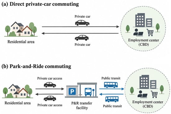
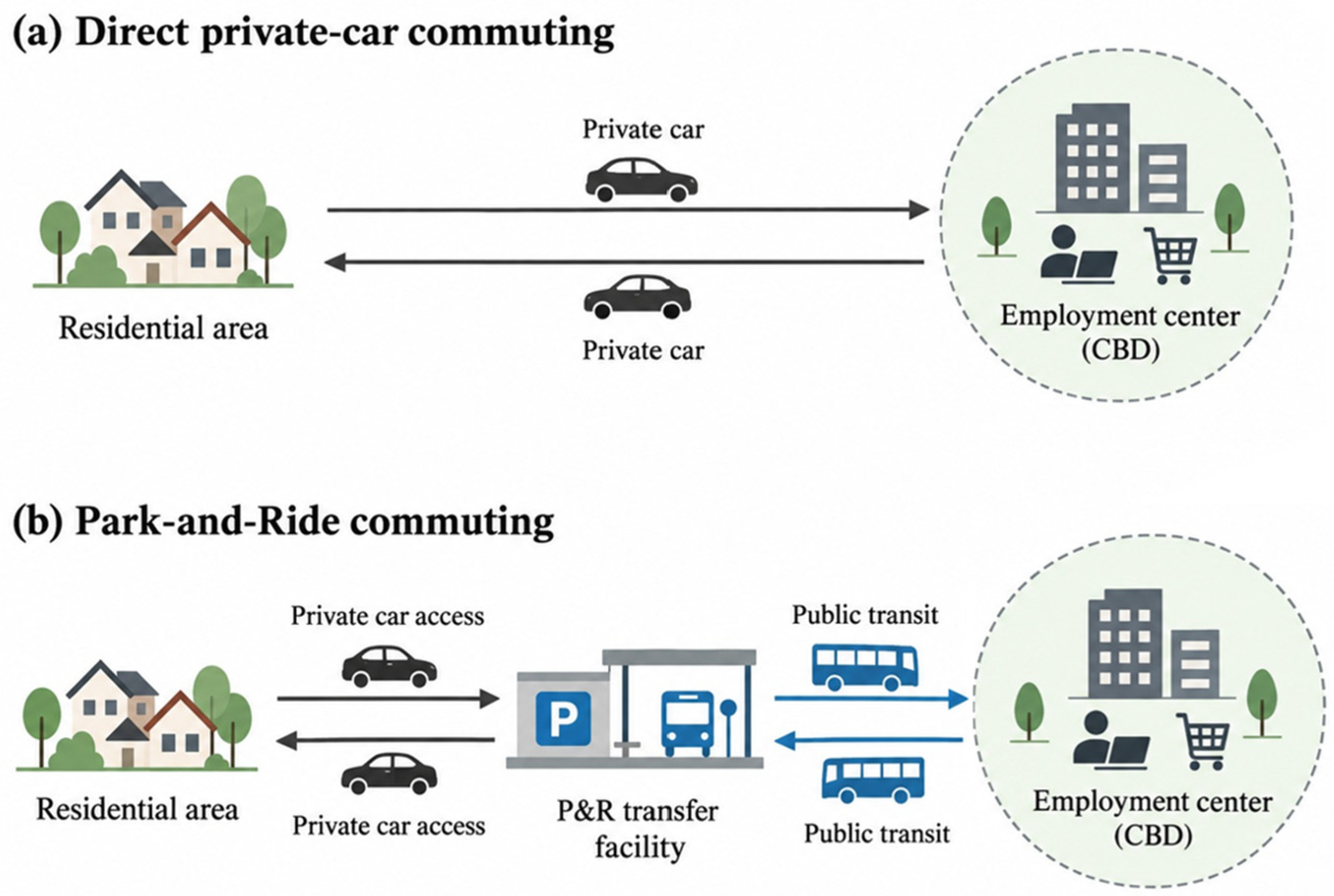
The spatial separation between low-density residential areas and concentrated employment centers in the Central Business District (CBD) generates substantial commuting demand and contributes to road congestion and parking pressure in central areas. As illustrated in Figure 1a, the conventional commuting pattern relies entirely on private cars for travel between residential areas and the CBD. In contrast, Figure 1b shows the P&R commuting pattern, in which travelers drive from residential areas to a P&R transfer facility and then continue their trips to the CBD by public transit. Given the OD demand, this study determines the locations of P&R facilities to enhance P&R demand capture and improve accessibility while accounting for travelers’ choice behavior and the spatial distribution of demand.

Figure 1. Commuting patterns: private car vs. P&R.

3.2. Modeling

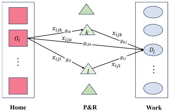
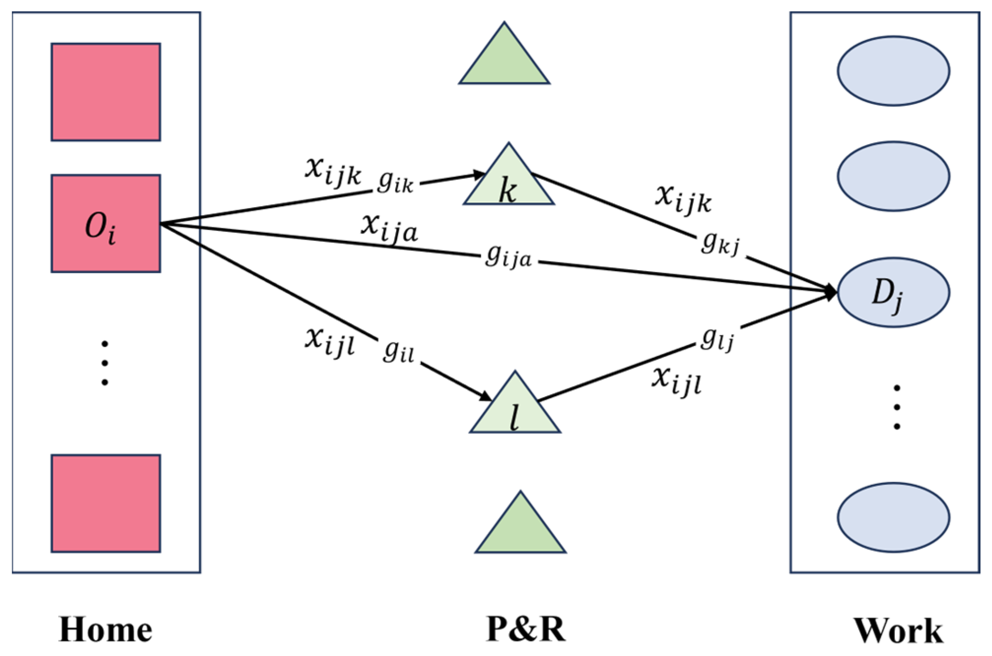
Figure 2 illustrates two travel options for each origin–destination (i, j) pair: direct private car travel and P&R. Each OD pair has a demand h_ij. In the private car mode, travelers incur a cost g_ija, proportional to distance. In the P&R mode, travelers drive to a candidate facility k ∈ K, then transfer to public transit, with total cost g_ijk = g_ik + g_kj. Facility construction is indicated by binary variable y_k. A multinomial Logit model determines the choice probability: x_ijk for P&R via facility k, and x_ija for direct car travel. This framework optimizes facility location to shift demand toward public transit and reduce urban congestion. The main notations are summarized in Table 1.

Figure 2. Mode choice structure and cost components in the P&R system.

Table 1. Summary of the main notations.

Sets
I:	set of origins concerning OD
J:	set of destinations concerning OD
K:	set of candidate facility
P:	set of extremum points
R:	set of extreme rays
Parameters
hij:	demand for OD between (i,j)
gijk:	cost of using facility k from i to j
θ:	cost sensitivity
p:	number of facilities constructed
a:	private car mode only
Variables
xijk:	continuous. proportion of OD pair (i,j) using facility k
xija:	continuous. proportion of OD pair (i,j) using mode a
yk:	binary. 1 if facility k is constructed, otherwise 0.
ya:	binary. 1 if mode a is selected, otherwise 0
λijk:	continuous. dual variable
μij:	continuous. dual variable
πijkl:	continuous. dual variable
zij:	introduced intermediate variable

The following assumptions are adopted to maintain model tractability:

(1)

The OD demand is assumed to be known.

(2)

Facility capacity constraints are not considered.

(3)

Travel costs are fixed, exogenous inputs based on Euclidean distances in the synthetic experiments and network shortest-path distances in the Chicago Sketch case study.

(4)

Traveler choices satisfy the Independence of Irrelevant Alternatives (IIA) assumption.

The IIA assumption implies that the odds of choosing one alternative over another do not depend on the availability of other alternatives. In P&R planning, nearby facilities may share access routes or transit services and thus be correlated substitutes. The present MNL specification does not explicitly represent this correlation and may overestimate their combined attractiveness, potentially affecting demand capture and facility selection. The analysis therefore focuses on exact optimization under the specified MNL model; mathematical optimality does not establish the empirical accuracy of its behavioral predictions.

Travelers’ choices depend on the generalized costs of the available alternatives and their sensitivity to these costs. Under the IIA assumption, the multinomial logit model estimates the probability that travelers associated with each OD pair choose a P&R facility or direct car travel. The multinomial logit model applies utility maximization under the independence assumption to estimate the probability that an OD pair (i,j) selects facility k or private car travel.

$$x_{\mathit{ijk}}={\displaystyle \frac{e^{-\theta g_{\mathit{ijk}}}}{\sum _{\forall l\in K\cup \left\{a\right\}}{e}^{-\theta g_{\mathit{ijl}}}}}\forall i\in I,\forall j\in J,\forall k,l\in K\cup \left\{a\right\},k\ne l$$

(1)

Here, the numerator is the perceived utility of commuters from origin i to destination j via facility k, and the denominator sums the utilities of all facilities plus the private car. Since constructed facilities are unknown, the binary variable y_k is introduced, and Equation (1) is accordingly reformulated as Equation (2).

$$x_{\mathit{ijk}}={\displaystyle \frac{y_k{e}^{-\theta g_{\mathit{ijk}}}}{\sum _{\forall l\in K\cup \left\{a\right\}}{y}_l{e}^{-\theta g_{\mathit{ijl}}}}}\forall i\in I,\forall j\in J,\forall k,l\in K\cup \left\{a\right\},k\ne l$$

(2)

If a facility at location k is not built (y_k = 0), then x_ijk = 0. The variable y_a = 1 always represents private car use, ensuring that the denominator is never zero. The parameter θ denotes cost sensitivity: a larger θ means users prefer cheaper modes. If a facility k is built, demand from OD pair (i,j) equals h_ijx_ijk; thus, total P&R demand is the sum over all OD pairs. The objective is to select p facilities from candidate set K to maximize total P&R users. The model is given as follows:

$$\mathit{max}\sum _{\forall i\in I,j\in J}\sum _{\forall k\in K}{h}_{\mathit{ij}}{x}_{\mathit{ijk}}$$

(3)

$$s.t.\sum _{\forall k\in K}{y}_k=p$$

(4)

y_a = 1

(5)

$$x_{\mathit{ijk}}={\displaystyle \frac{y_k{e}^{-\theta g_{\mathit{ijk}}}}{\sum _{\forall l\in K\cup \left\{a\right\}}{y}_l{e}^{-\theta g_{\mathit{ijl}}}}}\forall i\in I,\forall j\in J,\forall k,l\in K\cup \left\{a\right\},k\ne l$$

(6)

y_kϵ{0,1}   ∀k ∈ K

(7)

The above model describes a nonlinear integer problem. After linearization, the model is equivalent to the following:

$$\mathit{max}\sum _{\forall i\in I,j\in J}\sum _{\forall k\in K}{h}_{\mathit{ij}}{x}_{\mathit{ijk}}$$

(8)

$$s.t.\sum _{\forall k\in K}{y}_k=p$$

(9)

y_a = 1

(10)

x_ijk ≤ y_k   ∀i ∈ I, ∀j ∈ J, ∀k ∈ K ∪ {a}

(11)

$$x_{\mathit{ija}}+\sum _{\forall k\in K}{x}_{\mathit{ijk}}=1\forall i\in I,\forall j\in J$$

(12)

$$x_{\mathit{ijk}}\le {\displaystyle \frac{e^{-\theta g_{\mathit{ijk}}}}{\sum _{\forall l\in K\cup \left\{a\right\}}{e}^{-\theta g_{\mathit{ijl}}}}}{x}_{\mathit{ijl}}+\left(1-y_l\right)\forall i\in I,\forall j\in J,\forall k,l\in K\cup \left\{a\right\},k\ne l$$

(13)

0 ≤ x_ijk ≤ 1   ∀i ∈ I,∀j ∈ J,∀k ∈ K ∪ {a}

(14)

y_kϵ{0,1}   ∀k ∈ K

(15)

Objective function (8) maximizes facility usage. Constraint (9) restricts construction to p facilities from K. Constraint (10) sets private car share to 1, ensuring the denominator is nonzero. Constraint (11) links allocation to constructed facilities. Constraint (12) requires all mode shares to sum to 1. Constraint (13) enforces logit proportionality. Constraints (14) and (15) impose non-negativity and integrality. The linearization process of the above model was proposed by Aros-Vera et al. [11], and the complete proof can be found in their paper.

4. Solution Algorithm

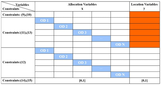
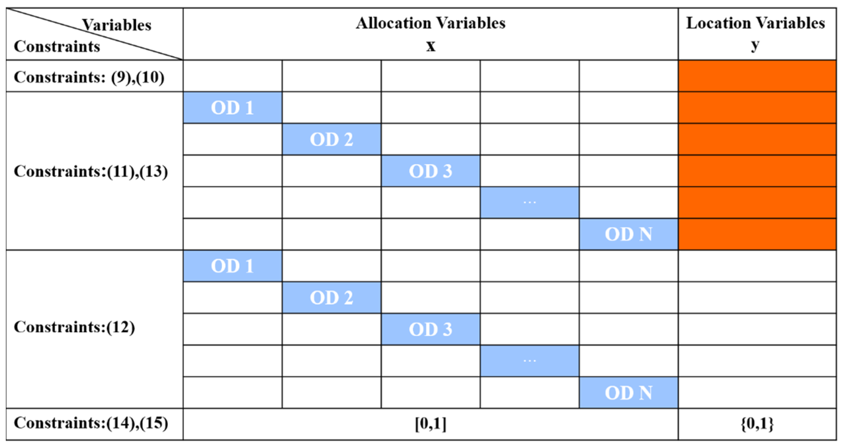
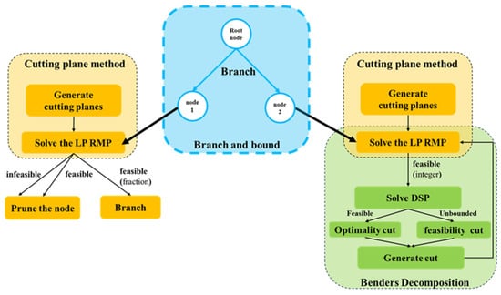
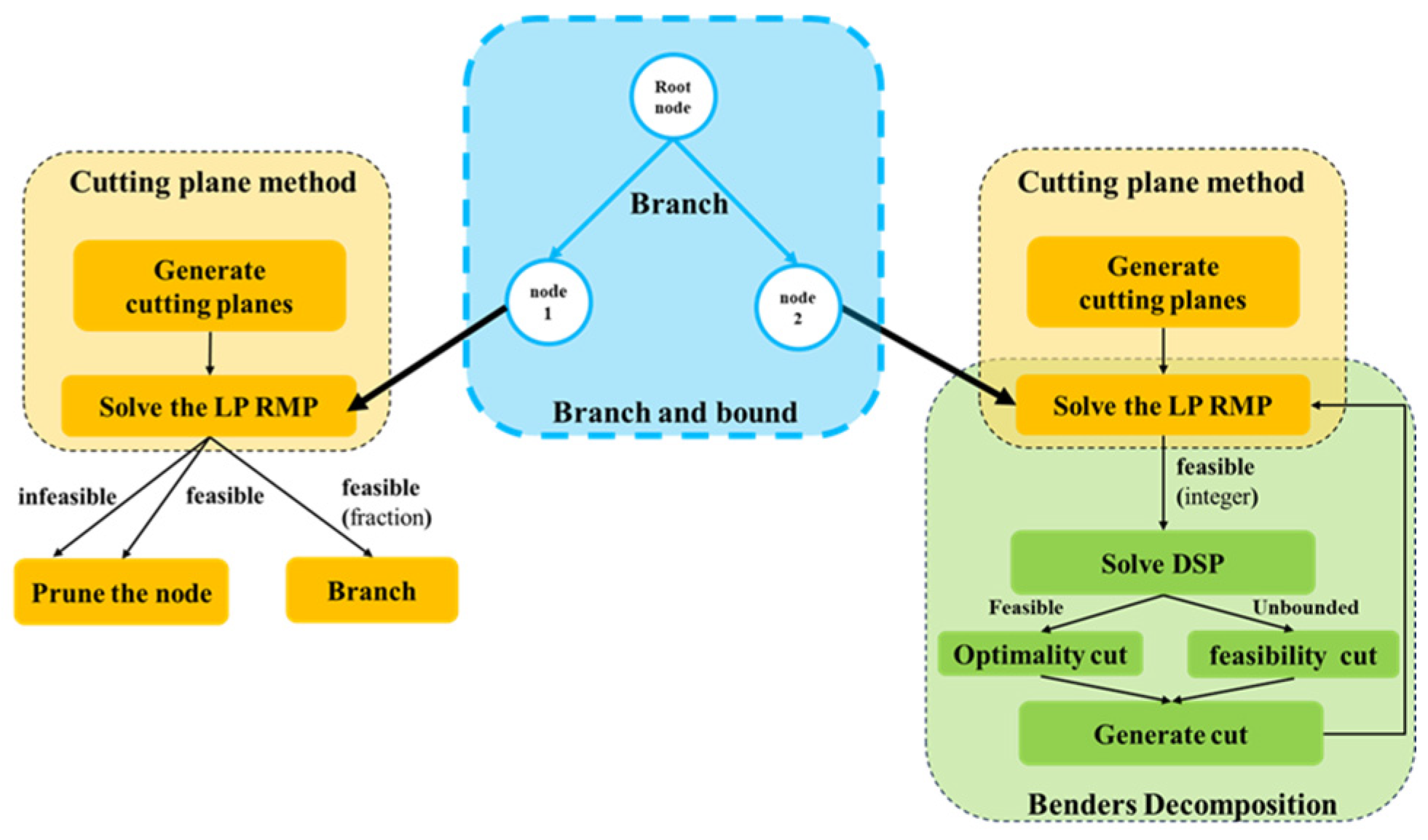
This study formulates the P&R facility location as a MILP with a block-diagonal structure, as illustrated in Figure 3, explicitly incorporating discrete choice behavior. The model tightly couples facility location and user flow assignment through probabilistic constraints, significantly increasing complexity and limiting the scalability of direct solver approaches. To address this, we propose a B&CBD algorithm based on the CBD framework. The model is decomposed into a relaxed master problem (RMP) and OD-specific Benders subproblems (BSPs), enabling reduced per-iteration complexity and parallel solutions. Unlike CBD, which suffers from slow convergence and large master problems, B&CBD integrates Benders cut generation into a branch-and-bound framework, allowing dynamic cut management and flexible branching. In addition, the in–out strategy described in Section 4.2 is used to generate Benders optimality cuts for the RMP; no additional family of strengthening inequalities is introduced. This yields a scalable and efficient algorithm tailored to the combinatorial complexity of large-scale mixed-integer optimization. A schematic of the B&C process with Benders decomposition is provided in Figure 4.

Figure 3. Structure of coupling constraints.

Figure 4. Schematic representation of Branch-and-Benders-Cut algorithm.

4.1. Classical Benders Decomposition

Based on the MILP established for the P&R facility location problem, it is known that the 0-1 integer variable indicates whether facility k is constructed, and the continuous variable represents the proportion of commuters traveling from origin i to destination j using facility k or driving private cars. The RMP contains integer variables, while the BSPs contain continuous variables. An overbar denotes a specified solution value. The vector $\overline{y_k}$ represents the current master-problem solution and is held fixed when solving the subproblem. The quantities ${\overline{{\lambda }_{\mathit{ijk}}}}^p$, ${\overline{{\mu }_{\mathit{ij}}}}^p$, and ${\overline{{\pi }_{\mathit{ijkl}}}}^p$ denote the dual-variable values associated with extreme point p ∈ P, which are used as coefficients in a Benders optimality cut. The RMP and BSP formulations of the MILP are given in Equations (16)–(20) and (21)–(25), respectively, as follows:

$$\left[\mathit{RMP}\right]\mathit{max}\sum _{\forall i\in I,j\in J}{z}_{\mathit{ij}}$$

(16)

$$s.t.\sum _{\forall k\in K}{y}_k=p$$

(17)

$$\sum _{\forall i\in I,j\in J}\sum _{\forall k\in K\cup \left\{a\right\}}{\overline{{\lambda }_{\mathit{ijk}}}}^p\overline{y_k}+\sum _{\forall i\in I,j\in J}{\overline{{\mu }_{\mathit{ij}}}}^p+\sum _{\forall i\in I,j\in J}\sum _{\forall k,l\in K\cup \left\{a\right\},l\ne k}{\overline{{\pi }_{\mathit{ijkl}}}}^p\left(1-\overline{y_k}\right)\ge z_{\mathit{ij}}p\in P$$

(18)

y_a = 1

(19)

y_kϵ{0,1}, z_ij   free   ∀i ∈ I, ∀j ∈ J, ∀k ∈ K

(20)

$$\left[\mathit{BSPs}\right]\mathit{max}\sum _{\forall i\in I,j\in J}\sum _{\forall k\in K}{h}_{\mathit{ij}}{x}_{\mathit{ijk}}$$

(21)

$$s.t.x_{\mathit{ijk}}\le \overline{y_k}\forall i\in I,\forall j\in J,\forall k\in K\cup \left\{a\right\}$$

(22)

$$x_{\mathit{ija}}+\sum _{\forall k\in K}{x}_{\mathit{ijk}}=1\forall i\in I,\forall j\in J$$

(23)

$$x_{\mathit{ijk}}\le {\displaystyle \frac{e^{-\theta g_{\mathit{ijk}}}}{\sum _{\forall l\in K\cup \left\{a\right\}}{e}^{-\theta g_{\mathit{ijl}}}}}{x}_{\mathit{ijl}}+\left(1-\overline{y_l}\right)\forall i\in I,\forall j\in J,\forall k,l\in K\cup \left\{a\right\},k\ne l$$

(24)

0 ≤ x_ijk ≤ 1   ∀i ∈ I, ∀j ∈ J, ∀k ∈ K ∪ {a}

(25)

Given the facility-location decisions obtained from the RMP, the BSP corresponding to each OD pair can be formulated as shown in Equations (21)–(25). Since each BSP is a linear programming problem, we solve its dual formulation, referred to as the dual Benders subproblem (DBSP). In the DBSP, the fixed facility-location decisions y_k affect only the objective function rather than the constraints. Therefore, at each iteration, only the objective function needs to be updated, while the constraint structure remains unchanged. Accordingly, the DBSPs are formulated as follows:

$$[\mathit{DBSPs}]\mathit{min}\sum _{\forall i\in I,j\in J}\sum _{\forall k\in K\cup \left\{a\right\}}{\lambda }_{\mathit{ijk}}\overline{y_k}+\sum _{\forall i\in I,j\in J}{\mu }_{\mathit{ij}}+\sum _{\forall i\in I,j\in J}\sum _{\forall k,l\in K\cup \left\{a\right\},l\ne k}{\pi }_{\mathit{ijkl}}(1-\overline{y_k})$$

(26)

$$s.t.{\lambda }_{\mathit{ijk}}+{\mu }_{\mathit{ij}}+\sum _{\forall l\in K\cup \left\{a\right\}}{\pi }_{\mathit{ijkl}}(1-{\displaystyle \frac{e^{-\theta g_{\mathit{ijl}}}}{e^{-\theta g_{\mathit{ijk}}}}}{\pi }_{\mathit{ijlk}})\ge h_{\mathit{ij}}\forall i\in I,\forall j\in J,\forall k\in K$$

(27)

$${\lambda }_{\mathit{ijk}}+{\mu }_{\mathit{ij}}+\sum _{\forall l\in K}{\pi }_{\mathit{ijkl}}(1-{\displaystyle \frac{e^{-\theta g_{\mathit{ijl}}}}{e^{-\theta g_{\mathit{ijk}}}}}{\pi }_{\mathit{ijlk}})\ge 0\forall i\in I,\forall j\in J,k=\{a\}$$

(28)

λ_ijk ≥ 0,   μ_ij free,   π_ijkl ≥ 0   ∀i ∈ I, ∀j ∈ J, ∀k,l ∈ K ∪ {a}

(29)

To simplify the interaction between the master problem and the subproblem, the dual form of the subproblem is further reformulated into a standard linear minimization problem, hereafter referred to as the reformulated dual of subproblems (RDBSPs).

$$[\mathrm{RDBSPs}]\max \sum _{\forall i\in I,j\in J}{z}_{\mathit{ij}}$$

(30)

$$s.t.\sum _{\forall i\in I,j\in J}\sum _{\forall k\in K\cup \left\{a\right\}}{\overline{{\lambda }_{\mathit{ijk}}}}^p\overline{y_k}+\sum _{\forall i\in I,j\in J}{\overline{{\mu }_{\mathit{ij}}}}^p+\sum _{\forall i\in I,j\in J}\sum _{\forall k,l\in K\cup \left\{a\right\},l\ne k}{\overline{{\pi }_{\mathit{ijkl}}}}^p\left(1-\overline{y_k}\right)\ge z_{\mathit{ij}}\forall p\in P$$

(31)

$$\sum _{\forall i\in I,j\in J}\sum _{\forall k\in K\cup \left\{a\right\}}{\overline{{\lambda }_{\mathit{ijk}}}}^r\overline{y_k}+\sum _{\forall i\in I,j\in J}{\overline{{\mu }_{\mathit{ij}}}}^r+\sum _{\forall i\in I,j\in J}\sum _{\forall k,l\in K\cup \left\{a\right\},l\ne k}{\overline{{\pi }_{\mathit{ijkl}}}}^r\left(1-\overline{y_k}\right)\ge 0\forall r\in R$$

(32)

z_ij   free

(33)

For this maximization problem, solving the RMP, a solution y^* can be obtained, and the optimal RMP objective value provides an upper bound on the original problem. At a feasible integer facility-location vector, solving the BSPs yields a feasible objective value and hence a lower bound. If the DSPs have an optimal solution and the upper and lower bounds are not equal, an optimality cut (inequality 31) can be added to the RMP. If the dual problem of the subproblem is unbounded, a feasibility cut (inequality 32) can be added to the RMP. The bounds are updated iteratively, and the iteration stops when their gap satisfies the prescribed tolerance. The CBD algorithm process is shown as Algorithm 1.

Algorithm 1. Pseudocode for classical benders decomposition algorithm.

Input: problem instance

Output: optimal site selection

1. Initialize: fix complicating variables y, set lower bound LB and upper bound UB and select value of ε

2. While UB−LB ≥ ε

3. Solve RDBSPs with current value of y*

4. If DSPs are unbounded then

5. Add feasibility cut (inequality 32) to the RMP

6. else

7. Update LB using the best feasible objective value obtained from the subproblems

Add optimality cut (inequality 31) to the RMP

8. end if

9. Solve RMP

Extract updated y* from solution

Update UB using the optimal RMP objective value

10. End while

11. Stop. Optimal solution of the original problem is obtained

4.2. Acceleration Strategy

CBD’s efficiency is often hampered by weak or poorly placed cuts, leading to slow convergence. To improve convergence, we adopt the in–out cut generation strategy originally proposed by Ben-Ameur and Neto [48] and subsequently applied by Fischetti et al. [49] and Song et al. [50]. The strategy strengthens Benders cuts by generating them at an interpolated separation point. The interpolation parameter is fixed at α = 0.5 for all instances.

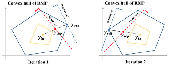
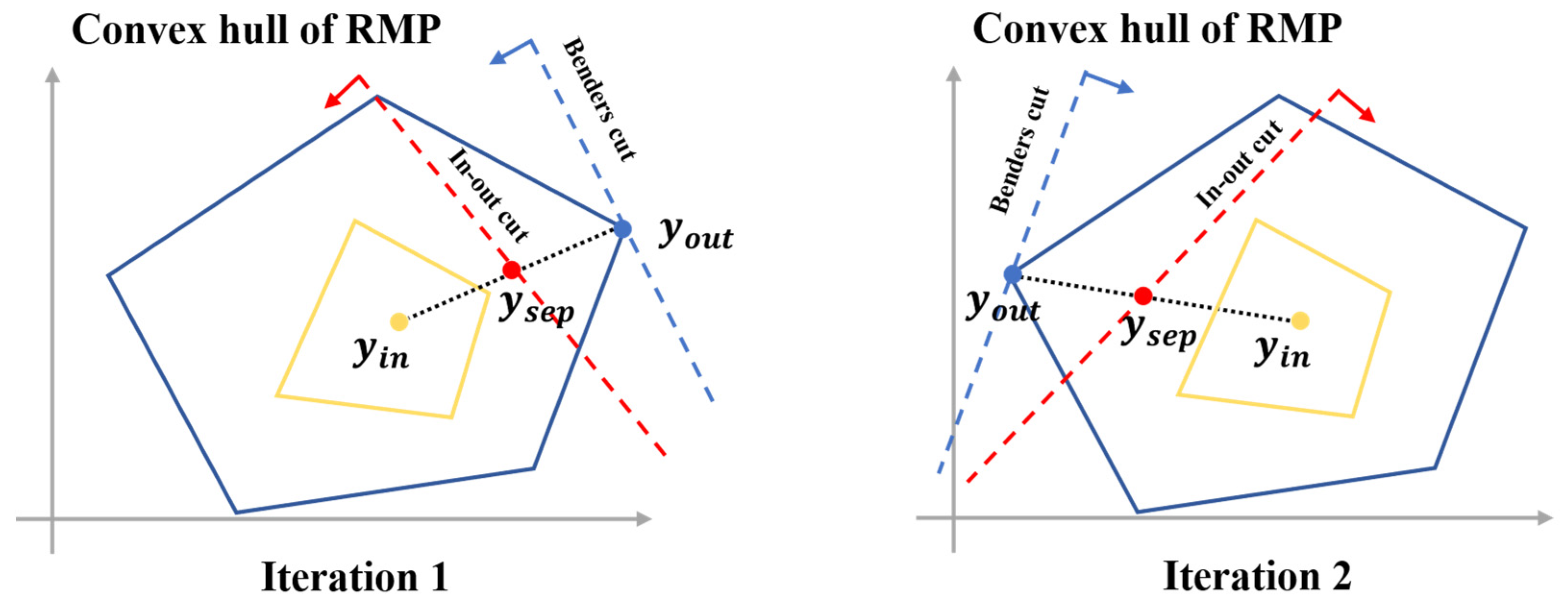
At each node, instead of generating cuts solely at the current RMP solution y_out and the feasible solution y_in of the original problem, we compute a separation point: y_sep = αy_out + (1 − α)y_in, α ∈ [0, 1]. This technique stabilizes the search and guides cut generation toward promising regions. As shown in Figure 5, cuts generated at y_sep typically separate both y_sep and y_out, improving efficiency. If no violated cuts are found, y_in is updated to y_sep for the next iteration. Specifically, the Benders optimality cut generated at y_sep, based on the dual solution (${\overline{{\lambda }_{\mathit{ijk}}}}^p,{\overline{{\mu }_{\mathit{ij}}}}^p,{\overline{{\pi }_{\mathit{ijkl}}}}^p$) of the subproblem, is formulated as follows:

$$\sum _{\forall i\in I,j\in J}\sum _{\forall k\in K\cup \left\{a\right\}}{\overline{{\lambda }_{\mathit{ijk}}}}^p{y}_{\mathit{sep}}+\sum _{\forall i\in I,j\in J}{\overline{{\mu }_{\mathit{ij}}}}^p+\sum _{\forall i\in I,j\in J}\sum _{\forall k,l\in K\cup \left\{a\right\},l\ne k}{\overline{{\pi }_{\mathit{ijkl}}}}^p\left(1-y_{\mathit{sep}}\right)\ge z_{\mathit{ij}}$$

(34)

Figure 5. In–out cutting plane schematic.

This form ensures that the optimality cut remains valid and effective, while the interpolation enhances numerical stability and cut strength.

4.3. Branch-and-Benders-Cut Decomposition Algorithm

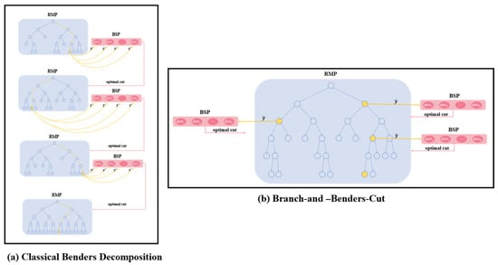
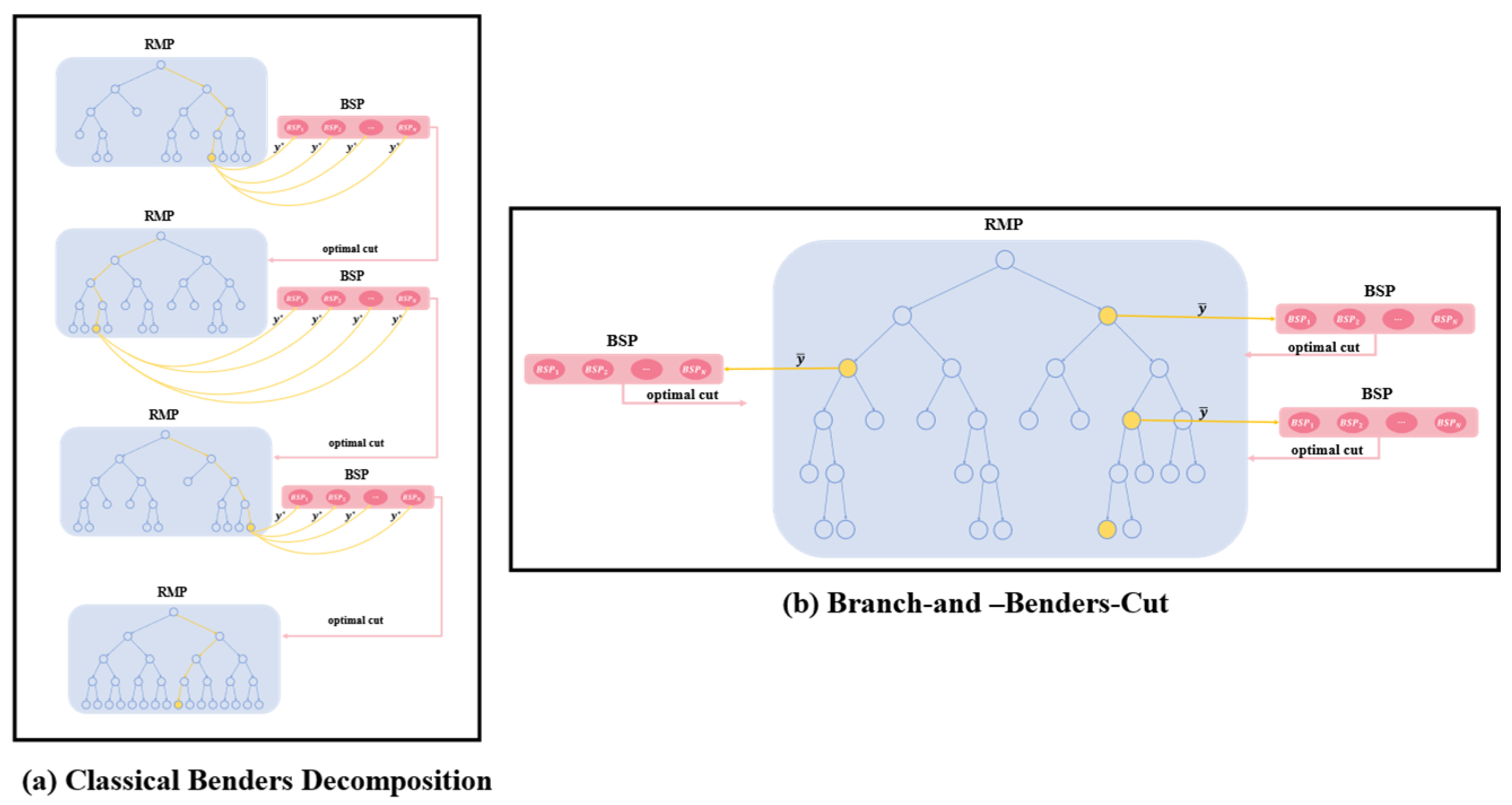
In traditional Benders decomposition, the RMP must be re-solved whenever a new cut is added. As cuts accumulate, the RMP grows, increasing computational overhead. Early iterations often generate weak cuts, leading to repeated exploration of similar solution regions and low efficiency. Although convergence is theoretically guaranteed, redundant computations and premature discarding of suboptimal solutions frequently occur. Figure 6 illustrates these limitations by contrasting CBD with the B&C framework, which avoids repeated master problem solving and enables more efficient cut management.

Figure 6. Comparison between classical Benders decomposition and the Branch-and-Benders-Cut framework.

In response, the B&CBD algorithm integrates Benders cuts directly into the branch-and-bound process. Unlike the traditional “Benders loop,” which requires solving the RMP to optimality at each iteration, B&C builds the RMP once and embeds cut generation and pruning within a single tree via callback functions. This prevents revisiting nodes and eliminates unnecessary restarts, significantly improving convergence efficiency. The framework has demonstrated strong performance in complex problems such as crew scheduling, time-dependent vehicle routing, stochastic network design, and the TSP with drones, highlighting its versatility and potential. Algorithm 2 presents the pseudocode of the B&CBD algorithm.

Algorithm 2 follows the maximization formulation. The node LP objective z is an upper bound for that node, whereas the incumbent objective z^* represents the best feasible objective value and hence a global lower bound. The incumbent objective is initialized to negative infinity and is updated only from a feasible integer solution whose subproblems have been evaluated. A node is pruned when its upper bound does not exceed the incumbent objective.

Algorithm 2. Pseudocode for B&CBD algorithm.

Input: problem instance, RMP, and DSP.

Output: final site-selection solution and its objective value.

1. Add the original RMP into tree L, initialize the incumbent solution y* = null, and its objective value z* = −∞.

2. While L is not empty do:

3. Select a node RMP from L.

4. Solve the LP relaxation of RMP to obtain an optimal solution $\overline{y}$ with objective value z.

5. If LP is infeasible, prune the node

6. Else if z ≤ z*, prune the node.

7. Else if $\overline{y}$ is integer:

8. Solve DSP based on $\overline{y}$ and generate benders cuts.

If no cuts generated, update z*= z and $y^{*}=\overline{y}$, prune the node.

Else, add the cuts to the LP relaxation and return to 4.

9. Else:

10. If a candidate solution $\widehat{y}$ is found, search for violated cutting planes.

Solve DSP based on $\widehat{y}$ and generate benders cuts.

If any cutting planes or benders cuts are found, add them to the LP relaxation and return to 4.

End if, choose one non-integral variable from $\overline{y}$ to branch, create two nodes and add them

11. end if

12. End while

13. Stop. Return Final solution y* and value of z*

5. Numerical Experiments

5.1. Experiment Setup and Evaluation Strategy

The computational evaluation compares B&CBD with CBD and CBD-I to examine convergence, solution bounds, and runtime. The direct solution of the complete MILP provides an additional baseline for the small synthetic instances. These comparisons distinguish improvements over other Benders variants from performance relative to direct solver optimization. The Chicago Sketch Network case study then examines the applicability of B&CBD to a larger network-based instance.

5.2. Small-Scale Instances

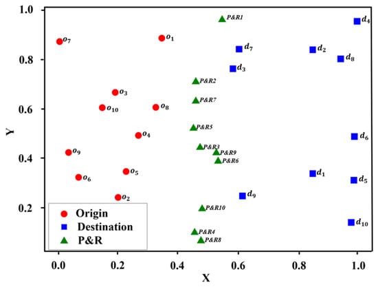
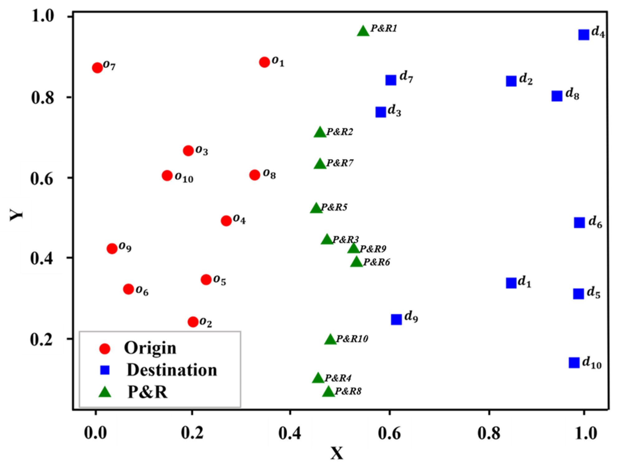
To test the proposed algorithm, a synthetic instance with 10 origins, 10 destinations, and 10 candidate facilities was generated. Coordinates were assigned within specific intervals to place facilities between origins and destinations. Travel costs in this synthetic instance are constructed from Euclidean distances between the generated coordinates, with direct car travel always being the cheapest. This setting provides a controlled geometric environment for comparing the solution algorithms and does not represent travel distances on a road network. The instance contains 100 OD pairs, each with demand 10. Figure 7 illustrates the spatial distribution, with circles for origins, squares for destinations, and triangles for facilities.

Figure 7. Distribution of origins, destinations, and P&R facilities.

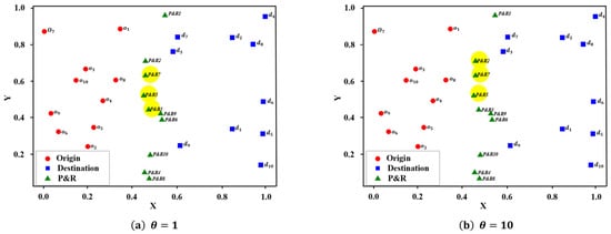
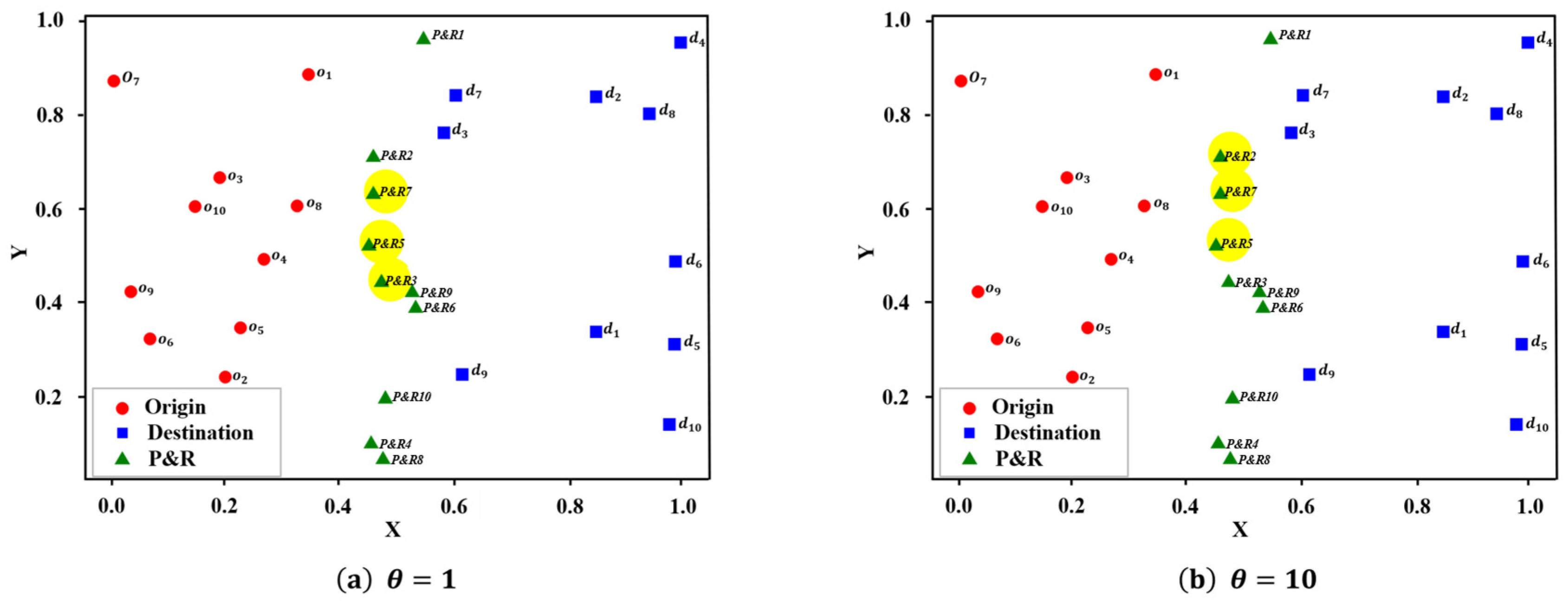
Figure 8 shows CBD solutions under different θ values. When θ = 1, facilities 3, 5, and 7 are selected, and Table A1, Table A2, Table A3 and Table A4 in Appendix A illustrate balanced mode choices, with OD pair (o1,d7) distributed across car and facilities 3, 5, and 7. As θ increases to 10, cost sensitivity rises, travelers favor direct car travel, and optimal facilities shift to 2, 3, and 5. Table A5, Table A6, Table A7 and Table A8 in Appendix A confirm this trend: a higher θ reduces P&R usage, while a more dispersed facility layout shortens access distance and better adapts to cost-sensitive conditions.

Figure 8. Facility location results under different θ values.

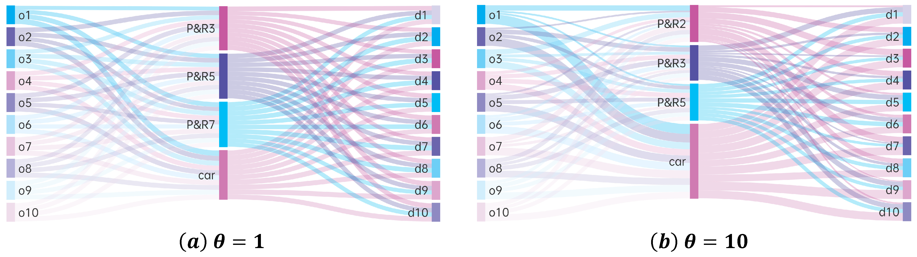
From the Sankey diagram in Figure 9 and Table 2, it is clear that as θ increases, commuters become more cost-sensitive and favor private cars, since costs are based on Euclidean distance. Car usage rises significantly—for instance, on the o2 − d9 route from 31% to 80%—while P&R usage falls, with facility pr7 dropping to 0% at θ = 10. This reflects commuters’ preference for direct routes over intermediate facilities. Consequently, facilities located farther from straight-line paths lose attractiveness as cost sensitivity grows, highlighting the need to incorporate user cost sensitivity into facility layout and planning.

Figure 9. Distribution of facility usage under different θ values.

Table 2. Origin–destination comparison for different levels of θ.

	θ = 1		θ = 10
	o2 − d9	o3 − d10	o2 − d9	o3 − d10
P&R2	-	-	0	12
P&R3	26	25	15	29
P&R5	24	25	5	29
P&R7	19	24	-	-
car	31	26	80	30

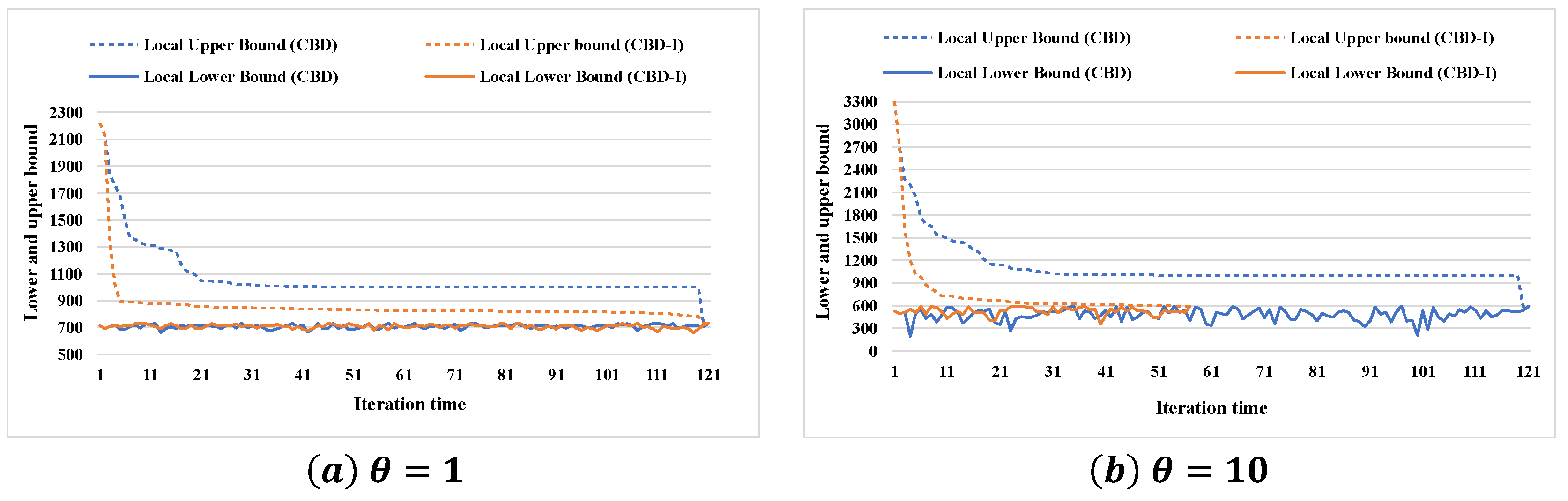
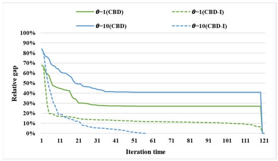
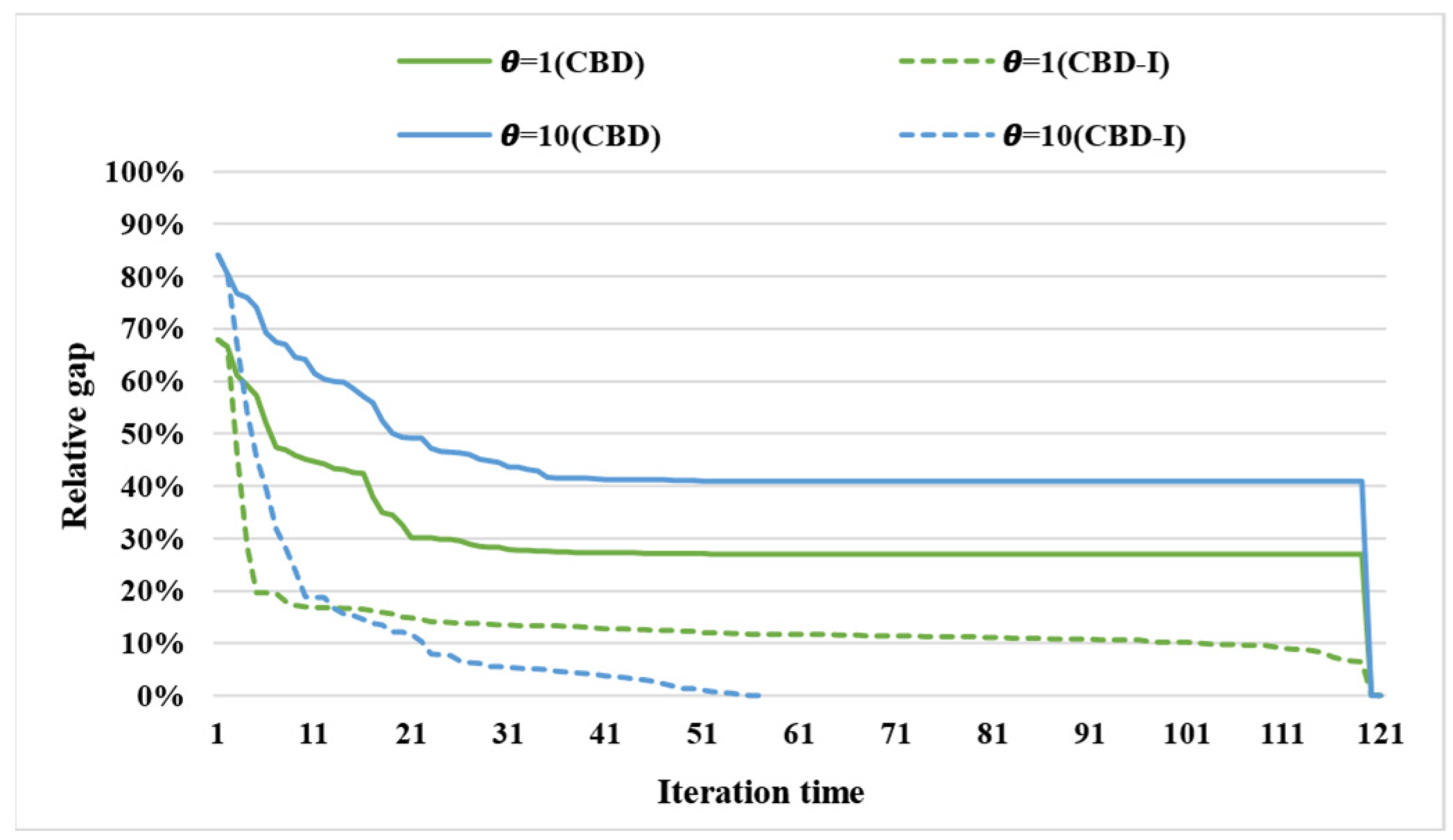
The convergence behavior of the CBD algorithm and the Benders decomposition algorithm with acceleration strategies under different θ values is illustrated in Figure 10. When θ = 1, the Benders decomposition algorithm with acceleration strategies significantly improves the lower bound in fewer iterations, but the total time required to reach convergence is comparable to that of the CBD algorithm. However, when θ = 10, the acceleration strategy substantially reduces the number of iterations needed to achieve convergence. Table 3 shows that CBD-I does not uniformly reduce runtime. A plausible explanation is that additional separation and subproblem effort can outweigh savings from improved cut selection and fewer iterations; the net benefit depends on the instance and parameter setting. Figure 11 shows the variation in the relative gap under different θ values. It indicates that, with the acceleration strategy, the relative gap value decreases rapidly in a short time. However, even when the relative gap value reaches zero, additional iterations are still required to achieve full convergence.

Figure 10. Convergence of upper and lower bounds under different θ values.

Table 3. Solution for different instances (total demand = 1000).

θ	p = 2						p = 3						p = 4
	Opt	P&R	B&C (s)	CBD (s)	CBD-I (s)	B&CBD (s)	Opt	P&R	B&C (s)	CBD (s)	CBD-I (s)	B&CBD (s)	Opt	P&R	B&C (s)	CBD (s)	CBD-I (s)	B&CBD (s)
0.1	664.7	5-7	3.10	24.7	46.9	4.9	748.2	3-5-7	6.82	234.7	388.1	13.9	798.3	2-3-5-7	13.48	1039.4	976.5	23.5
0.5	656.9	5-7	3.21	26.3	47.4	5.0	740.9	3-5-7	8.36	341.1	444.5	13.6	791.9	2-3-5-7	21.00	1115.1	1043.6	26.3
1	647.0	5-7	3.95	26.4	43.9	5.0	731.8	3-5-7	14.13	329.2	422.4	13.9	783.6	2-3-5-7	24.41	801.4	730.8	23.7
2	627.0	5-7	5.72	27.4	49.6	5.1	712.9	3-5-7	14.27	313.9	428.3	13.9	766.9	2-3-5-7	25.10	1096.7	915.8	24.3
3	607.1	5-7	5.62	25.1	47.3	5.1	694	3-5-7	14.55	321.2	362.6	14.1	750.2	2-3-5-7	18.75	1198.7	929.7	23.8
4	587.7	5-7	5.51	24.8	44.3	5.1	675.4	3-5-7	10.45	289.3	323.5	14.2	733.8	2-3-5-7	11.26	1058.4	1043.6	24.2
5	569.1	5-7	5.02	26.3	41.9	5.2	657.7	2-3-5	7.57	305.7	317.2	14.2	718.1	2-3-5-7	9.85	938.2	813.9	24.0
6	551.6	5-7	4.89	26.4	37.1	5.4	642.2	2-3-5	7.67	296.1	308.2	14.1	703	2-3-5-7	9.24	1078.2	531.7	24.2
7	535.2	5-7	3.86	26.4	34.2	5.2	627.8	2-3-5	7.82	285.8	255.3	14.3	688.8	2-3-5-7	6.63	833.8	526.7	24.7
8	519.9	5-7	3.15	25.8	33.4	5.2	614.5	2-3-5	7.99	290.0	291.9	14.1	675.7	2-5-6-7	7.27	823.3	450.9	23.9
9	508.4	2-3	3.19	25.4	30.0	5.3	602.1	2-3-5	6.43	312.7	187.5	13.8	664.4	2-3-6-7	6.39	824.2	283.7	24.3
10	497.8	2-3	2.98	24.7	27.8	5.2	590.6	2-3-5	4.04	300.2	136.5	14.2	653.9	2-3-6-7	5.62	835.0	312.6	24.4

Note: B&C was run using CPLEX 22.1.2 and Python 3.12.3 on Windows 11 (Intel Core Ultra 7 155H, 32 GB RAM), with one thread, a 3600 s time limit, and a relative gap tolerance of 1 × 10⁻⁶.

Figure 11. Relative gap values for different θ values.

Table 3 reports objective values, selected facilities, and solution times for CBD, CBD-I, B&CBD, and the direct MILP baseline (B&C) across 36 combinations of p and θ.

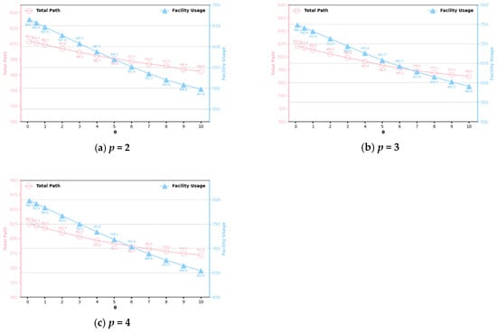
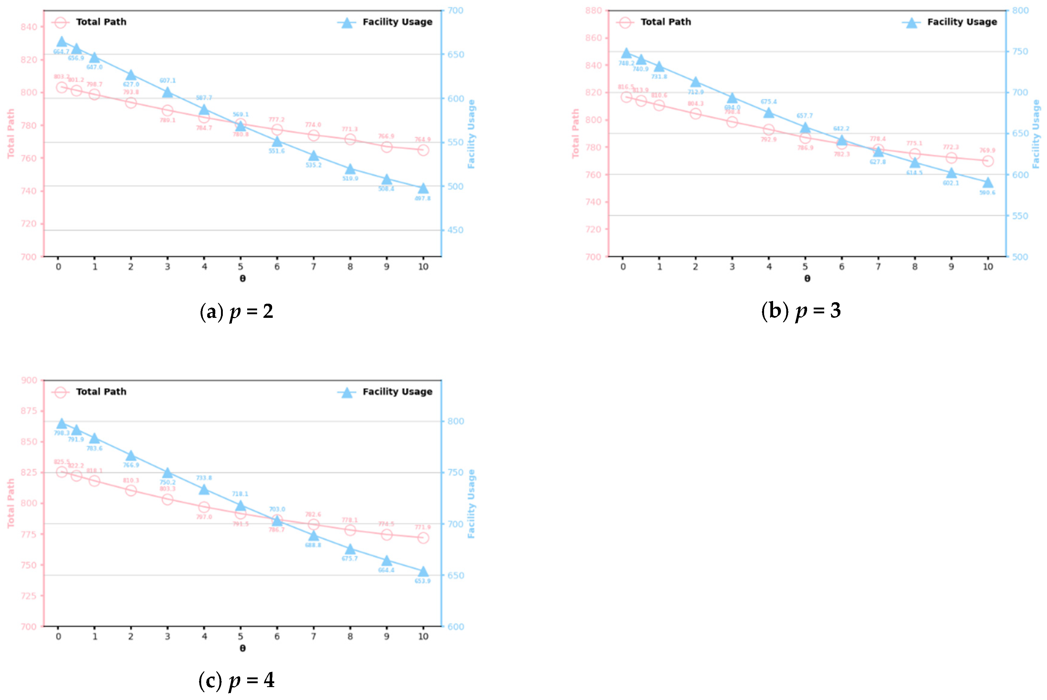
Figure 12 shows that P&R facility usage declines as θ increases, reflecting stronger traveler cost sensitivity. When costs rise, commuters tend to favor cheaper and more direct private car travel, reducing reliance on P&R facilities and impacting their efficiency and sustainability. At the same time, total travel distance decreases, as travelers avoid detours or transfers. This behavior highlights the close link between cost sensitivity and mode choice, suggesting that policymakers should account for these preferences when planning P&R systems and public transit to ensure effective, sustainable, and user-oriented transportation policies.

Figure 12. Trend of facility usage and total travel distance with changes in θ under different p values.

Table 3 shows that B&CBD requires less time than CBD and CBD-I for all reported small-scale instances. However, its advantage over these decomposition variants does not extend uniformly to the direct MILP baseline. According to the runtimes reported in Table 3, B&CBD is faster than B&C in 8 of the 36 parameter combinations, whereas B&C is faster in the remaining 28. For example, at p = 2 and θ = 2, the reported times are 5.1 s for B&CBD and 5.72 s for B&C; at p = 4 and θ = 10, they are 24.4 s and 5.62 s, respectively. Thus, B&CBD exhibits an advantage in a subset of the reported cases, but direct solution is generally faster at this scale. A plausible explanation is that, for these small instances, the overhead of solving Benders subproblems, generating cuts, and managing their integration into the search tree may outweigh the computational savings from decomposition. Consequently, the potential benefits of exploiting the OD-specific structure may not be fully realized at this scale. This interpretation motivates the Chicago Sketch Network test in Section 5.3, which increases the number of candidate facilities from 10 to 20 and the number of OD pairs from 100 to 340. The case study evaluates whether the approach remains applicable to a larger network-based problem.

5.3. Chicago Sketch Network

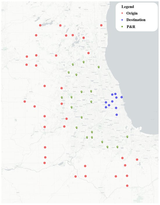
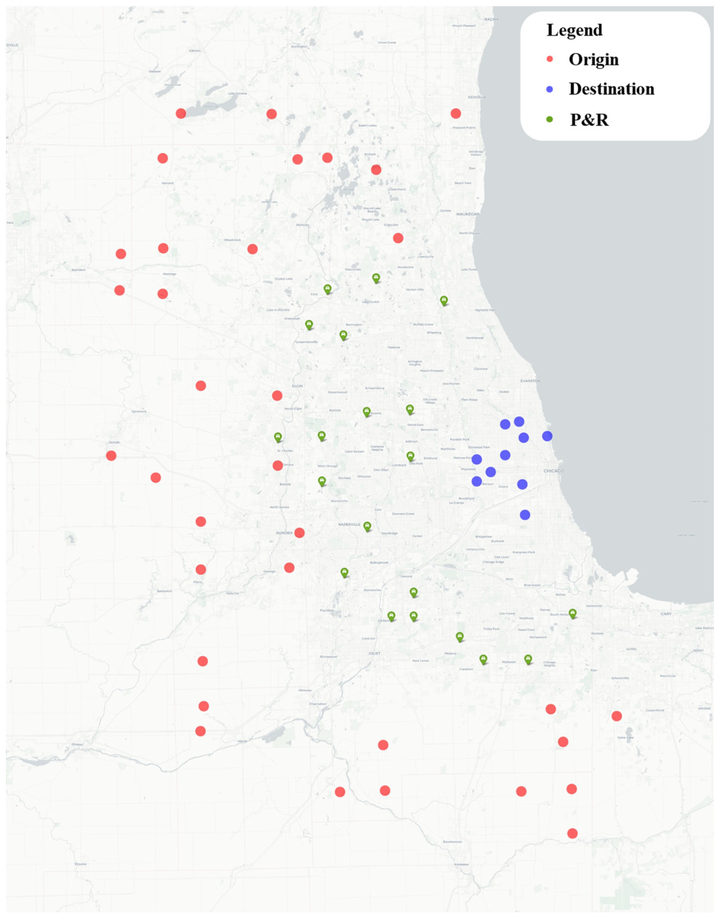
The Chicago Sketch Network was developed by the Chicago Area Transportation Study (CATS), a former regional transportation planning organization serving the Chicago metropolitan area. The network contains 933 nodes and 2950 links and provides a benchmark for transportation optimization. The 20 candidate P&R locations were manually selected from actual Chicago Sketch Network nodes and fixed before optimization, representing potential rather than confirmed existing facilities. In this case, 20 candidate P&R facilities are evaluated, with the goal of selecting five to maximize captured demand. The experimental instance comprises 34 suburban origins and 10 downtown destinations, yielding 340 OD pairs through all origin–destination combinations. Each OD pair is assigned a demand of 10 trips, giving a total demand of 3400 trips. The network and the locations of origins, destinations, and candidate P&R facilities are based on real-world spatial data, whereas OD demand is assumed for the computational experiments and is not derived from observed travel records. The resulting network configuration is shown in Figure 13.

Figure 13. Spatial distribution of origins, destinations, and candidate P&R facilities in the Chicago Sketch Network.

Unlike the synthetic experiments, this case study uses network shortest-path distances computed using Dijkstra’s algorithm to construct the travel-cost inputs. Network shortest-path distances account for network connectivity, whereas Euclidean distances measure geometric separation. The resulting costs are calculated before optimization and remain fixed during the solution process. This changes the input cost values rather than the algebraic structure of the optimization model. The problem is solved with the proposed B&CBD algorithm. By decomposing facility location and trip allocation within a B&C framework, the algorithm reduces redundant computation and ensures optimality. Because the two experimental settings use different distance-based cost representations, differences in predicted P&R capture and facility selection cannot be attributed solely to instance size; they also reflect spatial configuration, network connectivity, and the resulting cost inputs.

5.3.1. Computational Experiment Design

To distinguish the size of the underlying road network from the size of the optimization model, the scale experiments vary the number of OD pairs and candidate facilities. Twelve instances combine 100, 200, or 340 OD pairs with 10 or 20 candidate facilities and p = 3 or 5, with θ fixed at 1. Both B&C and B&CBD use the same demand and travel-cost inputs for each instance. The 933 road-network nodes are used to construct shortest-path costs and do not directly determine the number of facility-location variables.

As reported in Table 4, B&CBD reaches the prescribed optimality tolerance in all 12 instances, whereas B&C reaches it in 10 instances. With 10 candidate facilities, B&CBD is faster in the p = 3 cases, while direct MILP solution is faster in the p = 5 cases. With 20 candidates, B&CBD is faster in all six reported instances. For example, in S11, the reported times are 559.0 s for B&CBD and 3165.4 s for B&C. In S10 and S12, B&C retains gaps of 10.0% and 12.2%, respectively, while B&CBD closes its own bounds. Finding the same captured demand therefore does not imply that both methods have independently proved optimality. These results indicate that the benefit of decomposition depends on the instance structure and becomes more evident in the reported experiments with 20 candidate facilities.

Table 4. Computational results for the Chicago network instances.

Instance	OD Pairs	Candidates	p	B&C						B&CBD
				Captured Demand	LB	UB	Gap (%)	Time (s)	Status	Captured Demand	LB	UB	Gap (%)	Time (s)	Status
S01	100	10	3	713.6	713.6	713.6	0.0	3.3	Optimal	713.6	713.6	713.6	0.0	2.8	Optimal
S02	100	10	5	803.3	803.3	803.3	0.0	3.9	Optimal	803.3	803.3	803.3	0.0	6.5	Optimal
S03	200	10	3	1426.0	1426.0	1426.0	0.0	7.1	Optimal	1426.0	1426.0	1426.0	0.0	5.8	Optimal
S04	200	10	5	1606.1	1606.1	1606.1	0.0	18.9	Optimal	1606.1	1606.1	1606.1	0.0	23.9	Optimal
S05	340	10	3	2422.9	2422.9	2422.9	0.0	22.2	Optimal	2422.9	2422.9	2422.9	0.0	9.1	Optimal
S06	340	10	5	2729.8	2729.8	2729.8	0.0	21.5	Optimal	2729.8	2729.8	2729.8	0.0	22.5	Optimal
S07	100	20	3	729.0	729.0	729.0	0.0	217.6	Optimal	729.0	729.0	729.0	0.0	78.7	Optimal
S08	100	20	5	814.7	814.7	814.7	0.0	2973.6	Optimal	814.7	814.7	814.7	0.0	1292.2	Optimal
S09	200	20	3	1455.6	1455.6	1455.6	0.0	787.2	Optimal	1455.6	1455.6	1455.6	0.0	263.8	Optimal
S10	200	20	5	1628.0	1628.0	1791.0	10.0	10,799.1	Time limit	1628.0	1628.0	1628.0	0.0	7427.1	Optimal
S11	340	20	3	2475.6	2475.6	2475.6	0.0	3165.4	Optimal	2475.6	2475.6	2475.6	0.0	559.0	Optimal
S12	340	20	5	2708.0	2708.0	3039.0	12.2	10,799.3	Time limit	2708.0	2708.0	2708.0	0.0	8790.1	Optimal

Note: All instances use θ = 1 and 10 trips per OD pair. Both methods use CPLEX 22.1.2 with one thread, a 10,800 s time limit, and a 1 × 10⁻⁶. MIP gap tolerance. Times are actual wall-clock runtimes; Gap (%) = 100×max(0,UB-LB)/|LB|, using same-run bounds at termination. “Optimal” indicates optimality within tolerance.

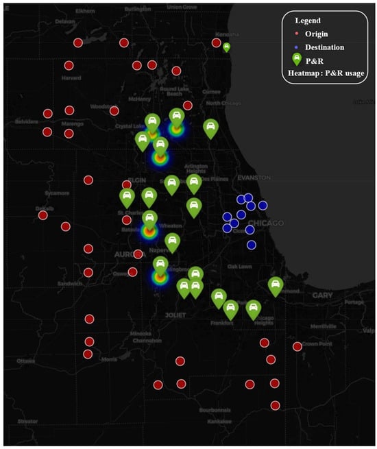
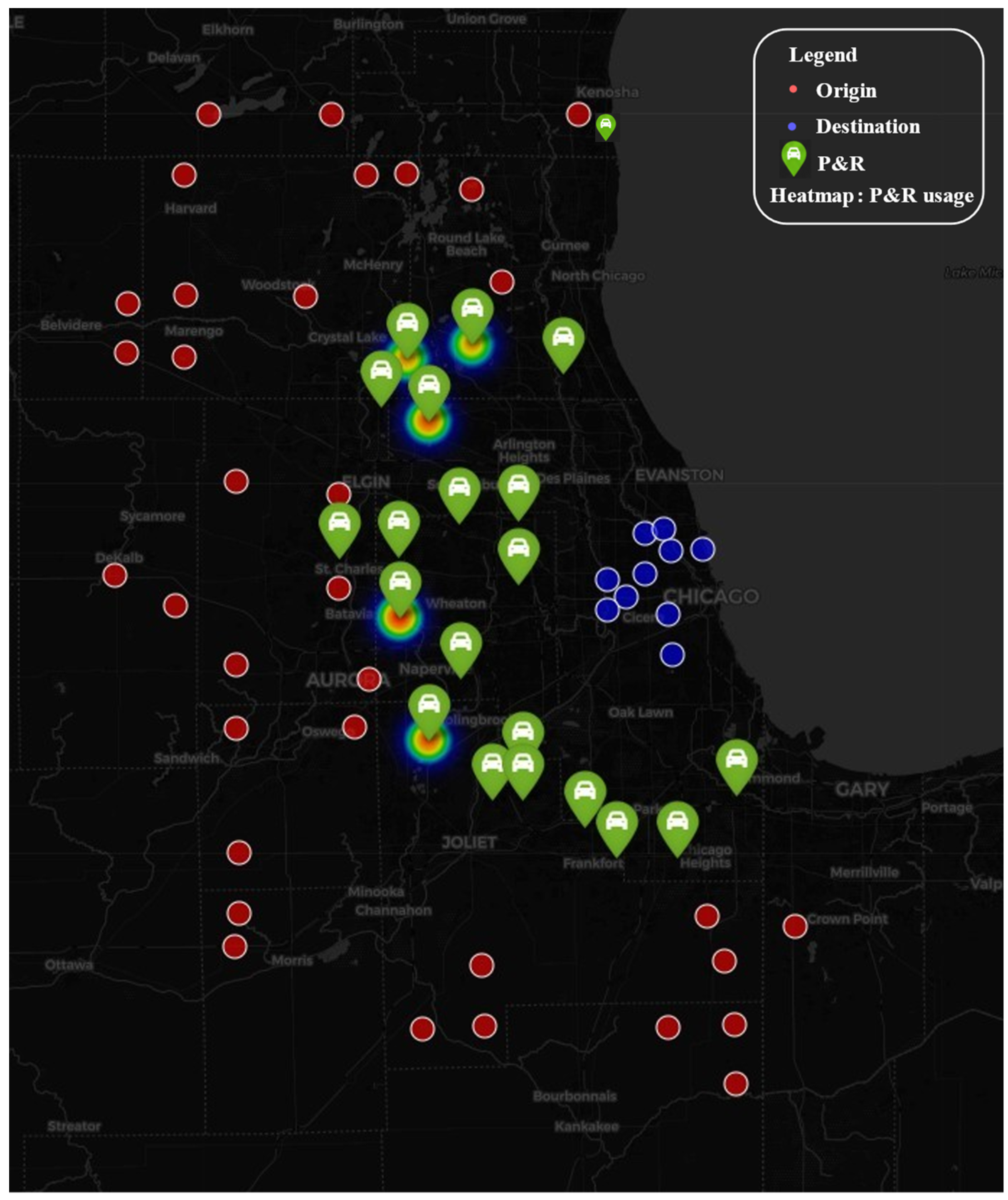
The results are shown in Figure 14. Five facilities at nodes 584, 686, 770, 808, and 811 were selected, capturing a total demand of 2708 trips. Their spatial distribution provides broad suburban coverage and suggests the potential to reduce downtown traffic and parking pressure. This application illustrates the use of B&CBD for the specified MNL-based P&R planning problem. The predicted demand capture and selected locations are conditional on the assumed costs and the MNL choice model and do not constitute an empirical validation of traveler behavior.

Figure 14. Locations of facilities and captured demand.

5.3.2. Sensitivity to the Cost-Sensitivity Parameter

The sensitivity experiments use 340 OD pairs, 20 candidate facilities, and a total demand of 3400 trips. Table 5 reports B&CBD results for p = 3 and 5 and θ = 0.1, 0.5, 1, 2, 5, and 10. Its bounds and gaps come from the corresponding B&CBD run.

Table 5. Sensitivity analysis of B&CBD on the Chicago network.

Instance	p	θ	Captured Demand	Capture Rate (%)	LB	UB	Gap (%)	Time (s)	Status	Network Node IDs
T01	3	0.1	2542.8	74.8	2542.8	2542.8	0.0	614.7	Optimal	584, 680, 692
T02	3	0.5	2513.5	73.9	2513.5	2513.5	0.0	609.8	Optimal	584, 680, 692
T03	3	1.0	2475.6	72.8	2475.6	2475.6	0.0	559.0	Optimal	584, 680, 692
T04	3	2.0	2396.1	70.5	2396.1	2396.1	0.0	651.8	Optimal	584, 680, 692
T05	3	5.0	2146.7	63.1	2146.7	2146.7	0.0	679.9	Optimal	584, 680, 692
T06	3	10.0	1818.4	53.5	1818.4	1818.4	0.0	685.4	Optimal	664, 680, 692
T07	5	0.1	2827.0	83.1	2827.0	3400.0	20.3	10,799.9	Time limit	584, 686, 702, 770, 808
T08	5	0.5	2801.2	82.4	2801.2	3400.0	21.4	10,799.9	Time limit	584, 686, 702, 770, 808
T09	5	1.0	2708.0	79.6	2708.0	2708.0	0.0	8790.0	Optimal	584, 686, 770, 808, 811
T10	5	2.0	2694.7	79.3	2694.7	2694.7	0.0	8130.5	Optimal	584, 686, 770, 808, 811
T11	5	5.0	2471.8	72.7	2471.8	3400.0	37.6	10,813.4	Time limit	664, 676, 702 770, 808
T12	5	10.0	2169.8	63.8	2169.8	3400.0	56.7	10,813.4	Time limit	664, 674, 692, 770, 808

Note: LB and UB are the feasible lower bound and global upper bound obtained from the same B&CBD run. Gap (%) = 100 × max(0,UB-LB)/|LB|. “Optimal” denotes optimality within the prescribed tolerance; time-limit results are not proven optimal.

The reported captured demand decreases as θ increases, consistent with stronger sensitivity to travel costs. For p = 3, it decreases from 2542.8 trips (74.8%) at θ = 0.1 to 1818.4 trips (53.5%) at θ = 10, and all six instances reach the prescribed tolerance. For p = 5, the reported values decrease from 2827.0 trips (83.1%) to 2169.8 trips (63.8%). Opening five rather than three facilities increases the reported captured demand at each tested θ. However, this comparison is between reported feasible solutions wherever a nonzero gap remains, rather than between proven optimal values.

Although the instance dimensions remain unchanged, varying θ changes the choice probabilities and constraint coefficients and can affect Benders convergence. As reported in Table 5, the p = 5 instances with θ = 1 and 2 reach the prescribed tolerance, while those with θ = 0.1, 0.5, 5, and 10 retain gaps at termination. Their upper bounds remain at the total demand of 3400, indicating difficulty in proving optimality rather than an inability to obtain feasible solutions. The selected nodes also vary across parameter settings, and the time-limit solutions should not be interpreted as proven optimal facility layouts. These findings demonstrate the applicability of the proposed framework to network-based P&R planning, while showing that its computational performance and predicted facility choices depend on the cost-sensitivity parameter.

6. Concluding Remarks

This study proposes an integrated optimization framework for the competitive P&R facility location problem by combining discrete-choice modeling with a B&CBD algorithm. The framework links facility location and demand allocation through the specified MNL choice probabilities while enabling the efficient solution of large-scale instances. Numerical experiments on different problem sizes and an application to the Chicago Sketch Network demonstrate the computational efficiency, scalability, and practical applicability of the proposed approach. The main conclusions are as follows:

(1)

Modeling framework: The MNL specification represents probabilistic traveler choice and competition among P&R facilities subject to the IIA assumption. By jointly considering facility-location and flow-allocation decisions, the formulation represents the interactions among facilities, travelers, and transportation demand. The original nonlinear mixed-integer model is reformulated as a mixed-integer linear program, enabling the use of exact optimization methods.

(2)

Algorithmic contribution: The proposed B&CBD algorithm embeds Benders decomposition within a B&C framework and dynamically generates feasibility and optimality cuts. By decomposing the location and allocation decisions, the algorithm reduces the size of the master problem and avoids redundant subproblem calculations. Subproblem decomposition and in–out cut generation further improve convergence and computational efficiency.

(3)

Computational results: B&CBD is faster than the tested Benders variants in the synthetic experiments, although the direct MILP solution is generally faster at this scale. In the 12 Chicago network-based instances, B&CBD reaches the prescribed tolerance in all cases, whereas the direct solution does so in 10. Its advantage is more evident in the reported instances with 20 candidates. Sensitivity results show that captured demand decreases with increasing cost sensitivity, while convergence varies with the parameter setting; results with nonzero gaps remain feasible solutions rather than proven optima.

This study uses distance-based proxies for travel costs: Euclidean distances in the synthetic experiments and network shortest-path distances in the Chicago Sketch case study. Although the latter account for network connectivity, the cost representation remains simplified and does not explicitly include waiting and transfer times. In addition, the behavioral parameters are not empirically calibrated, and facility capacities are assumed to be unlimited. Future research should incorporate real-world travel data, more comprehensive travel-cost structures, and facility-capacity constraints to improve the behavioral realism and practical applicability of the proposed framework.

A further limitation is the IIA assumption, particularly when candidate facilities are spatially close substitutes. Future work should examine nested or mixed logit specifications to represent correlated alternatives and preference heterogeneity, using observed choice data for estimation and validation. Such extensions would require reassessing the formulation and decomposition method; their compatibility with the present algorithm is not established here.

References

- Noel, E.C. Park-and-Ride: Alive, Well, and Expanding in the United States. J. Urban Plan. Dev. 1988, 114, 2–13. [Google Scholar] [CrossRef] [Scilit]
- Danilina, N.; Vlasov, D. Development of «Park-and-Ride» System as a Tool for Sustainable Access Control Managing. IOP Conf. Ser. Earth Environ. Sci. 2017, 90, 012214. [Google Scholar] [CrossRef] [Scilit]
- Horner, M.W.; Grubesic, T.H. A GIS-Based Planning Approach to Locating Urban Rail Terminals. Transportation 2001, 28, 55–77. [Google Scholar] [CrossRef] [Scilit]
- Holguín-Veras, J.; Reilly, J.; Aros-Vera, F.; Yushimito, W.; Isa, J. Park-and-Ride Facilities in New York City. Transp. Res. Rec. 2012, 2276, 123–130. [Google Scholar] [CrossRef] [Scilit]
- Yaliniz, P.; Ustun, O.; Bilgic, S.; Vitosoglu, Y. Evaluation of Park-and-Ride Application with AHP and ANP Methods for the City of Eskisehir, Turkey. J. Urban Plan. Dev. 2022, 148, 04021066. [Google Scholar] [CrossRef] [Scilit]
- Ortega, J.; Moslem, S. Decision Support System for Evaluating Park & Ride System Using the Analytic Hierarchy Process (AHP) Method. Urban Plan. Transp. Res. 2023, 11, 2194362. [Google Scholar] [CrossRef] [Scilit]
- Ortega, J.; Moslem, S.; Tóth, J.; Péter, T.; Palaguachi, J.; Paguay, M. Using Best Worst Method for Sustainable Park and Ride Facility Location. Sustainability 2020, 12, 10083. [Google Scholar] [CrossRef] [Scilit]
- Pitale, A.M.; Parida, M.; Sadhukhan, S. GIS-MCDM–Based Approach to Determine the Potential Facility Locations for Park-and-Ride Facilities along Transit Corridors. J. Urban Plan. Dev. 2022, 148, 05021065. [Google Scholar] [CrossRef] [Scilit]
- Fierek, S.; Bieńczak, M.; Zmuda-Trzebiatowski, P. Multiple Criteria Evaluation of P&R Lots Location. Transp. Res. Procedia 2020, 47, 489–496. [Google Scholar] [CrossRef] [Scilit]
- Akram, M.; Zahid, K.; Kahraman, C. A New ELECTRE-Based Decision-Making Framework with Spherical Fuzzy Information for the Implementation of Autonomous Vehicles Project in Istanbul. Knowl.-Based Syst. 2024, 283, 111207. [Google Scholar] [CrossRef] [Scilit]
- Aros-Vera, F.; Marianov, V.; Mitchell, J.E. P-Hub Approach for the Optimal Park-and-Ride Facility Location Problem. Eur. J. Oper. Res. 2013, 226, 277–285. [Google Scholar] [CrossRef] [Scilit]
- Haase, K.; Müller, S. A Comparison of Linear Reformulations for Multinomial Logit Choice Probabilities in Facility Location Models. Eur. J. Oper. Res. 2014, 232, 689–691. [Google Scholar] [CrossRef] [Scilit]
- Pang, H.; Khani, A. Modeling Park-and-Ride Location Choice of Heterogeneous Commuters. Transportation 2018, 45, 71–87. [Google Scholar] [CrossRef] [Scilit]
- Sharma, B.; Hickman, M.; Nassir, N. Park-and-Ride Lot Choice Model Using Random Utility Maximization and Random Regret Minimization. Transportation 2019, 46, 217–232. [Google Scholar] [CrossRef] [Scilit]
- Mather, J.J. Guidelines and Standards for the Planning, Design, and Operation of Bus Park-and-Ride Facilities. Transp. Res. Rec. 1983, 908, 1–6. [Google Scholar]
- Spillar, R.J. Park-and-Ride Planning and Design Guidelines; Parsons Brinckerhoff Inc.: New York, NY, USA, 1997. [Google Scholar]
- Coffel, K.; Transit Cooperative Research Program. Guidelines for Providing Access to Public Transportation Stations; Transportation Research Board: Washington, DC, USA, 2012. [Google Scholar]
- Cherrington, L.; Brooks, J.; Cardenas, J.; Elgart, Z.; Galicia, L.; Hansen, T.; Miller, K.; Walk, M.; Ryus, P.; Semler, C.; et al. Decision-Making Toolbox to Plan and Manage Park-and-Ride Facilities for Public Transportation: Guidebook on Planning and Managing Park-and-Ride; World Transit Research; Transportation Research Board: Washington, DC, USA, 2017. [Google Scholar]
- Mock, A.; Thill, J.-C. Placement of Rapid Transit Park-and-Ride Facilities. Transp. Res. Rec. 2015, 2534, 109–115. [Google Scholar] [CrossRef] [Scilit]
- Ortega, J.; Tóth, J.; Moslem, S.; Péter, T.; Duleba, S. An Integrated Approach of Analytic Hierarchy Process and Triangular Fuzzy Sets for Analyzing the Park-and-Ride Facility Location Problem. Symmetry 2020, 12, 1225. [Google Scholar] [CrossRef] [Scilit]
- Palevičius, V.; Grigonis, V.; Podviezko, A.; Barauskaitė, G. DEVELOPMENTAL ANALYSIS OF PARK-AND-RIDE FACILITIES IN VILNIUS. Promet-Traffic Transp. 2016, 28, 165–178. [Google Scholar] [CrossRef] [Scilit]
- Hakimi, S.L. Optimum Locations of Switching Centers and the Absolute Centers and Medians of a Graph. Oper. Res. 1964, 12, 450–459. [Google Scholar] [CrossRef] [Scilit]
- Church, R.; Velle, C.R. THE MAXIMAL COVERING LOCATION PROBLEM. Pap. Reg. Sci. 1974, 32, 101–118. [Google Scholar] [CrossRef] [Scilit]
- ReVelle, C.S.; Swain, R.W. Central Facilities Location. Geogr. Anal. 1970, 2, 30–42. [Google Scholar] [CrossRef] [Scilit]
- Hodgson, M.J. A Flow-Capturing Location-Allocation Model. Geogr. Anal. 1990, 22, 270–279. [Google Scholar] [CrossRef] [Scilit]
- Horner, M.W.; Groves, S. Network Flow-Based Strategies for Identifying Rail Park-and-Ride Facility Locations. Socio-Econ. Plan. Sci. 2007, 41, 255–268. [Google Scholar] [CrossRef] [Scilit]
- Mai, T.; Lodi, A. A Multicut Outer-Approximation Approach for Competitive Facility Location under Random Utilities. Eur. J. Oper. Res. 2020, 284, 874–881. [Google Scholar] [CrossRef] [Scilit]
- Freire, A.S.; Moreno, E.; Yushimito, W.F. A Branch-and-Bound Algorithm for the Maximum Capture Problem with Random Utilities. Eur. J. Oper. Res. 2016, 252, 204–212. [Google Scholar] [CrossRef] [Scilit]
- Ljubić, I.; Moreno, E. Outer Approximation and Submodular Cuts for Maximum Capture Facility Location Problems with Random Utilities. Eur. J. Oper. Res. 2018, 266, 46–56. [Google Scholar] [CrossRef] [Scilit]
- Méndez-Vogel, G.; Marianov, V.; Lüer-Villagra, A. The Follower Competitive Facility Location Problem under the Nested Logit Choice Rule. Eur. J. Oper. Res. 2023, 310, 834–846. [Google Scholar] [CrossRef] [Scilit]
- Liu, H.; Li, Y.; Li, J.; Hou, B.; Zhao, S. Optimizing the Location of Park-and-Ride Facilities in Suburban and Urban Areas Considering the Characteristics of Coverage Requirements. Sustainability 2022, 14, 1502. [Google Scholar] [CrossRef] [Scilit]
- Huang, Y.; Gan, H.; Lu, H.; Wang, X.; Wang, W. Park-and-Ride Choice Behaviour under Multimodal Travel Information—Analysis Based on Panel Mixed Logit Model. IET Intell. Transp. Syst. 2023, 17, 2063–2074. [Google Scholar] [CrossRef] [Scilit]
- Kitthamkesorn, S.; Chen, A.; Opasanon, S.; Jaita, S. A P-Hub Location Problem for Determining Park-and-Ride Facility Locations with the Weibit-Based Choice Model. Sustainability 2021, 13, 7928. [Google Scholar] [CrossRef] [Scilit]
- Kim, S.H.; Qiu, F.; Shim, S. Capacitated P-Hub Approach for Park-and-Ride Facility Location Problem under Nested Logit Demand Function: Polyhedral Approaches. Optim. Eng. 2026, 27, 1997–2028. [Google Scholar] [CrossRef] [Scilit]
- Song, Z.; He, Y.; Zhang, L. Integrated Planning of Park-and-Ride Facilities and Transit Service. Transp. Res. Part C Emerg. Technol. 2017, 74, 182–195. [Google Scholar] [CrossRef] [Scilit]
- Ruan, J.-M.; Liu, B.; Wei, H.; Qu, Y.; Zhu, N.; Zhou, X. How Many and Where to Locate Parking Lots? A Space–Time Accessibility-Maximization Modeling Framework for Special Event Traffic Management. Urban Rail Transit 2016, 2, 59–70. [Google Scholar] [CrossRef] [Scilit][Green Version]
- Wang, X.; Gan, H.; Wang, K.; Wang, W.; Huang, Y.; Lu, H. Understanding Park-and-Ride Decisions: The Influence of Travel Information, Values, and Attitudes. Transp. Res. Part F Traffic Psychol. Behav. 2025, 113, 326–343. [Google Scholar] [CrossRef] [Scilit]
- Wang, J.Y.T.; Yang, H.; Lindsey, R. Modelling Park-and-Ride Service in a Linear Monocentric City. Int. J. Urban Sci. 2004, 8, 74–89. [Google Scholar] [CrossRef] [Scilit]
- Khakbaz, A.; Nookabadi, A.S.; Shetab-bushehri, S.N. A Model for Locating Park-and-Ride Facilities on Urban Networks Based on Maximizing Flow Capture: A Case Study of Isfahan, Iran. Netw. Spat. Econ. 2013, 13, 43–66. [Google Scholar] [CrossRef] [Scilit]
- Farhan, B.; Murray, A.T. Siting Park-and-Ride Facilities Using a Multi-Objective Spatial Optimization Model. Comput. Oper. Res. 2008, 35, 445–456. [Google Scholar] [CrossRef] [Scilit]
- Henry, E.; Furno, A.; Faouzi, N.-E.E.; Rey, D. Locating Park-and-Ride Facilities for Resilient on-Demand Urban Mobility. Transp. Res. Part E Logist. Transp. Rev. 2022, 158, 102557. [Google Scholar] [CrossRef] [Scilit]
- Zhang, Y.; Xiao, Y.; Zhang, C.; Song, M.; Cheng, L. A Decomposition-Based Optimization Framework for Heterogeneous Multi-Compartment Vehicle Routing With Splittable Demand in Urban Cold Chain Logistics. IEEE Trans. Intell. Transp. Syst. 2026, 27, 8638–8651. [Google Scholar] [CrossRef] [Scilit]
- Méndez-Vogel, G.; Marianov, V.; Lüer-Villagra, A. Combining State-of-the-Art Row Generation Methods for the Competitive Facility Location Problem with Multinomial Logit Choice Rule. Omega 2025, 136, 103339. [Google Scholar] [CrossRef] [Scilit]
- Song, M.; Zhang, C.; Zhang, Y.; Cheng, L. A Solution Space Decomposition Method to Find the Best K Fixed-Charge Network Designs. Transp. Res. Rec. J. Transp. Res. Board 2025, 2679, 163–175. [Google Scholar] [CrossRef] [Scilit]
- Zhang, C.; Yong, R.; Jiang, X.; Zhang, Y.; Song, M.; Cheng, L. Benders Decomposition for Charging Station Location-Routing Problem with Time-Dependent Travel Times: A Space-Time-Electricity Network Perspective. Energy 2025, 333, 137310. [Google Scholar] [CrossRef] [Scilit]
- Zhang, C.; Xie, L.; Wu, Y.; Feng, T.; Cheng, L. A Two-Stage Stochastic Programming Approach for the Time-Dependent Vehicle Routing Problem with Stochastic Demands: A Dynamic Space–Time Network Perspective. Transp. Res. Part E Logist. Transp. Rev. 2026, 215, 105105. [Google Scholar] [CrossRef] [Scilit]
- Zhang, C.; Wu, Y.; Feng, T.; Zhang, Y.; Song, M.; Cheng, L. Benders Decomposition for Traveling Salesman Problem with Drone: A Space-Time-State Network Perspective. Transp. Res. Part C Emerg. Technol. 2025, 179, 105255. [Google Scholar] [CrossRef] [Scilit]
- Ben-Ameur, W.; Neto, J. Acceleration of Cutting-plane and Column Generation Algorithms: Applications to Network Design. Networks 2007, 50, 179–192. [Google Scholar] [CrossRef] [Scilit]
- Fischetti, M.; Ljubić, I.; Sinnl, M. Redesigning Benders Decomposition for Large-Scale Facility Location. Manag. Sci. 2017, 63, 2146–2162. [Google Scholar] [CrossRef] [Scilit]
- Song, M.; Cheng, L.; Ge, H.; Li, Y.; Sun, C. A Stabilizing Benders Decomposition Method for the Accessibility-Oriented Charging Station Location Problem. Sustain. Cities Soc. 2023, 94, 104558. [Google Scholar] [CrossRef] [Scilit]
Disclaimer/Publisher’s Note: The statements, opinions and data contained in all publications are solely those of the individual author(s) and contributor(s) and not of MDPI and/or the editor(s). MDPI and/or the editor(s) disclaim responsibility for any injury to people or property resulting from any ideas, methods, instructions or products referred to in the content. |
© 2026 by the authors. Licensee MDPI, Basel, Switzerland. This article is an open access article distributed under the terms and conditions of the Creative Commons Attribution (CC BY) license.