


Highlights
Please indicate how your work links to systems science via your contributions to systems practice, theory, and/or methodology.
- An empirically anchored hours module connects assumed household and employer pressure responses to labour, income and stock-flow-consistent macroeconomic feedbacks.
- Matched simulations distinguish the model-level effects of baseline work schedules, assumed pressure responses and market-share competition.
What are the main findings and/or the implications of the main findings?
- Under market-share competition, positive income-gap pressure alone raises simulated output and lowers unemployment, whereas adding employer pressure lengthens hours but lowers output and raises unemployment.
- Magnitudes and welfare conclusions depend on specification: an upper-tail hours cost cuts the pressure-related hours increase from 13.75 to 6.13 h per week, and valuing non-market time amplifies the welfare loss only when unemployment is weighted more than in the reference index.
Abstract
We study how assumed pressure responses shape work hours, macroeconomic outcomes and welfare in a China-calibrated agent-based stock-flow-consistent model that combines a 2017 social accounting matrix with a 2016 CFPS schedule anchor. Household income-gap and employer-pressure loadings are scenario inputs rather than estimates; 1320 supplementary runs vary their signs and test the model’s mechanisms. Negative employer loadings reverse the hours response, and macroeconomic outcomes are not monotone in hours: under market-share competition, income-gap pressure alone raises output and lowers unemployment, whereas adding employer pressure lengthens hours, lowers output and raises unemployment. At the central loadings, pressure raises mean hours under competition by 13.75 h, or by 6.13 h with an upper-tail hours cost; remaining saturation at the hours bound limits quantitative interpretation. The competition-associated output loss survives removing the above-anchor labour increment or the markup-pressure term, and the pressure-induced output reversal survives unifying consumption propensities or removing the direct wage squeeze; its wage–income counterpart reflects mainly employment losses. At the reference unemployment penalty, valuing non-market time does not amplify the competition welfare loss in any of 80 sampled designs; only higher, exploratory unemployment weights do. The model supports conditional scenario analysis, not causal or policy-effect estimates for China.
1. Introduction
Market-share competition and weak household demand can coexist in the same socio-economic system. Firms respond to weak sales by cutting margins and raising competitive expenditure, while households may respond to income and workplace pressure by changing hours. Measured activity may then rise even though the system sustains a fragile competitive position by spending more time rather than producing more value. A macroeconomic system that records employment but not hours cannot separate this intensive-margin escalation from an extensive-margin expansion, and a welfare index based only on consumption cannot value the associated loss of non-market time. Recent Chinese analysis characterises this “involutionary” competition precisely as homogeneous low-price rivalry, weak utilisation and profitability, and insufficient differentiation through innovation [1].
We treat that configuration as a system outcome and study it with an agent-based stock-flow-consistent (AB-SFC) macroeconomic system calibrated to China. The central question is narrow and conditional: under declared pressure responses, how does the work-hours channel change the output and welfare behaviour of market-share competition under weak household demand? The question links relative-income and rank-based incentives [2,3,4] to an agent-based stock-flow-consistent macro system [5,6]. We use “involution” only as a label for a specific measurable configuration—competitive effort and longer hours without a commensurate welfare gain—not as a stand-alone theory. Because the pressure responses are not identified by the available data (Section 4), we do not estimate them; we ask what system behaviour alternative response signs and magnitudes generate.
We make three contributions to the analysis of socio-economic systems. First, we add an explicit, empirically anchored mapping from household income gaps and employer competition pressure to weekly hours and transmit hours consistently to effective labour, wage income, consumption and non-market time while keeping private pressure incentives out of social welfare. Second, we combine hours/pressure ablations with signed coefficients and production/pricing switches to trace the labour-income–consumption–production–fiscal–financial circuit under controlled model changes. Third, we compare a consumption-only with a time-adjusted welfare index under declared ablations and functional forms, exposing where the welfare assessment depends on a normative accounting choice. Our work is a disciplined conditional counterfactual about system behaviour, not a causal estimate that competition raised Chinese hours by the modelled amount.
At the archived central loadings, pressure raises mean hours under competition by 13.75 h, and competition amplifies the pressure contrast by 10.30 h. An upper-tail hours cost reduces the former contrast to 6.13 h, so both specifications are reported. Because a positive utility shifter lengthens hours by construction, the hours sign is not itself evidence for the mechanism; the questions are how its magnitude depends on the hours rule and how the endogenous macroeconomic feedbacks respond.
Supplementary sensitivity and mechanism experiments (840 runs) extend the analysis beyond positive loadings. Negative employer-pressure coefficients reverse the hours response, and positive income-gap pressure alone raises output and lowers unemployment. The central competition-minus-demand output loss survives removing either the above-anchor effective-labour increment or the direct markup-pressure term, and it develops only after an initial output increase. An additional 480 four-cell runs retain the pressure-effect reversal after unifying base consumption propensities or removing the direct wage-squeeze multiplier. Production-stage wage accounting and firm-level capacity diagnostics narrow the explanation without identifying a unique causal chain.
At the reference unemployment weight, including non-market time does not amplify the competition-minus-demand welfare loss in any of the 80 sampled designs. Exploratory comparisons vary the unemployment-status weight , which well-being evidence motivates but does not identify in this model’s utility units. Changing the weight can change the ranking; relocating an unchanged penalty from the aggregate to each household cannot.
The scope is deliberately bounded. The model does not include health capital, burnout transitions, “lying-flat” states, household bargaining or multiple-job histories; those mechanisms are important but ancillary to the present systems analysis, and their explicit modelling and calibration are deferred to future work. The supporting information comprises Supplementary Sections S1–S10, Tables S1–S25 and Figures S1–S6; complete captions are listed in the Supplementary Materials statement.
2. Related Literature and Mechanism Gap
2.1. Positional Incentives and the Intensive Margin
The paper uses “involution” in a deliberately narrow economic sense. It does not treat the term as a stand-alone theory. The relevant mechanisms are older and more precise: rank-based rewards can affect effort incentives [3,7]; relative income and status provide background for studying consumption comparisons [2,4]; and a rat race can make excessive effort individually rational under a common institutional constraint [8]. Rank-based incentives do not by themselves imply socially excessive effort. In the present model, this family of mechanisms is represented by a household income shortfall and an employer-specific competition signal. An allocation is described as involutionary only when these pressures increase market work without a commensurate improvement in the reported consumption–time welfare measure.
The sign of a relative-income effect on labour supply is not automatic. Laboratory evidence shows that relative pay can change the supplied effort, but that the response depends on how the pay difference is explained [9]. Survey evidence likewise links perceived relative income to preferred hours and hours mismatch [10], while theory shows that reference dependence can create a wedge between micro and aggregate labour-supply responses [11]. Bowles and Park connect consumption emulation and inequality to longer work hours across countries [12]; Bell and Freeman emphasise promotion and future earnings as incentives for current hours in the United States and Germany [13]. These studies motivate a pressure channel but do not estimate our Chinese income-gap or employer-pressure loadings. We therefore examine both the positive-response region and a signed-coefficient grid that includes zero and negative responses.
2.2. Hours Are Jointly Constrained by Workers and Firms
Observed hours are an equilibrium object, not a transparent observation of a worker preference parameter. Pencavel [14] emphasises that a wage–hours relationship can mix worker supply and employer demand. This identification warning is especially relevant here because employer pressure is part of the question. The model therefore represents the hours decision as a reduced-form worker–employer outcome: household consumption and non-market time enter choice utility, but the employer’s price-competition state shifts the chosen schedule. The construction is not labelled a structural labour-supply estimate.
Long hours also need not translate one-for-one into productive services. Using worker-level variation in scheduled hours in a call centre, Collewet and Sauermann [15] find declining output per hour as working time rises. This evidence motivates considering diminishing productivity. In our illustrative alternative, hours beyond an individual’s baseline schedule have half the marginal productivity of baseline hours. Because payment rules are institution-specific, the sensitivity design separately considers proportional pay, a cap on paid additional hours, and a 1.5 overtime premium. The 0.5 productivity coefficient and 1.5 pay multiplier are scenario assumptions, not estimates from that study. These alternatives prevent the result from depending on an untested identity between time, output and earnings.
China’s work-time evidence also cautions against interpreting main-job hours as total work burden. The 1995 two-day-weekend reform reduced main-job weekly hours but induced some workers to take a second job and changed household work [16]. CFPS qg6 measures current-main-job weekly hours. The paper therefore calls non-market time, not observed leisure, and holds multiple-job and household-production mechanisms outside the model.
A parallel literature distinguishes the welfare consequences of unemployment from the value of voluntary non-market time. Unemployment carries non-pecuniary costs beyond income loss [17,18,19]. Past unemployment is associated with lower life satisfaction, although scarring and habituation need not imply a uniform permanent cost [20]. Knabe et al. [21] find lower experienced well-being within the same activities for unemployed people, but no significant difference in time-weighted daily experienced utility: time reallocation can offset the activity-specific disadvantage. Jahoda’s account of the latent functions of employment provides a theoretical background [22]. Retirement from long-term unemployment can raise life satisfaction, consistent with a change in employment norms and identity [23]; this does not establish that all non-pecuniary losses disappear. Chadi and Hetschko [24] likewise distinguish income-satisfaction losses from potential gains in satisfaction with free time and family life. Time-allocation and home-production theory motivate distinguishing the uses and opportunity costs of non-market time [25,26]. Employment status can enter preferences in different ways, but their signs and economic interpretations are not interchangeable. Fixed costs of work [27] and indivisible-labour models [28,29] concern the cost or allocation of employment, not a fixed disutility of non-employment. Search-and-matching models make the value of non-employment relevant to labour-market decisions [30,31] without supplying a value for here. The well-being literature therefore motivates an exploratory non-employment burden; because its translation into our consumption-normalised utility units requires additional assumptions, we treat the weight as a normative scenario parameter.
2.3. From Household Demand to Firm Competition
The work-hours channel is embedded in a weak-demand AB-SFC model. Buffer-stock saving under uncertainty [32] and household expenditure risks in China [33] motivate the demand block. A lower consumption propensity among wealthier households is a separate model assumption, examined by the propensity-homogeneity experiments below. When sales are weak, firms revise expected demand, prices, markups, investment and hiring. Activating market-share competition adds price-cut and competitive-expenditure pressure while keeping the demand shock fixed. Employees linked to those firms then receive a stronger hours signal. This link allows firm rivalry to affect both the number employed and the hours of those workers.
Hours and headcount need not substitute one for one. In the search-and-matching model of Marimon and Zilibotti [34], employment effects of reduced hours depend on preferences, wage adjustment and fixed hiring costs. Our adaptive headcount rule differs from negotiated work-sharing models: current hours do not enter the target-headcount denominator. The mechanism switches below therefore test particular production and pricing links within this closure, without identifying a general work-sharing effect.
The broader firm and credit blocks draw on the literature on excessive competition and delayed exit. Zombie lending can keep low-productivity firms alive, depress restructuring and congest product and credit markets [35]. Recovery is also possible: Fukuda and Nakamura [36] study how restructuring and changes in the macroeconomic environment helped Japanese zombie firms recover. Related evidence documents zombie firms and overcapacity in Chinese manufacturing [37]. Those features remain part of the macro environment, but the present analysis does not promote each baseline component to a separate contribution. They matter here insofar as they determine the employer-pressure state and preserve the balance-sheet feedbacks in which the hours experiment operates.
2.4. AB-SFC Method, Validation and Contribution
Stock-flow-consistent modelling requires each sectoral flow to map to a change in stocks and each financial asset to have a counterpart liability [5,38]. Agent-based SFC models add heterogeneous households, firms and banks while retaining those aggregate accounting constraints [6,39]. Agent-based macroeconomic surveys emphasise heterogeneous, out-of-equilibrium policy experiments rather than representative-agent aggregation [40,41], while labour-market applications show how SFC-ABMs can trace employment and distribution jointly [42]. Recent China-focused applications also use SFC or SFC multi-agent systems for macro-financial simulation and fiscal-policy comparison [43,44]. Their advantage for this question lies in mechanism transparency: the framework can remove one arrow at a time—the hours block, the pressure shift or market-share competition—while following the resulting labour-income, consumption, production, fiscal and financial flows. Forecasting precision is not the claim.
Within this class, the present model extends the AB–SFC benchmark of Caiani et al. [6]; Section 3.1 separates the retained backbone from the added mechanisms and parameterisation.
That flexibility creates a validation obligation. Pattern-oriented modelling requires a parameterisation to confront several empirical regularities rather than one selected target [45]. Informed by the broader discussion of empirical validation in Windrum et al. [46], we distinguish accounting validity, calibration fit and external evidence as an organising framework for this study. Explicit timing, state variables and replication materials also respond to the reporting and reproducibility concerns formalised in the updated ODD protocol [47]. The paper implements that separation as a five-part validation protocol: reproducible measurement, calibration to the 2016 h distribution, macro-fiscal validation, a no-re-estimation comparison with 2022, and a common-seed mechanism test with global sensitivity analysis. Each tool answers a narrow question. SFC residuals establish accounting closure; the 2022 comparison measures temporal transportability; seed intervals measure stochastic simulation variation. Separately or together, they do not amount to empirical validity, re-calibration or survey-design and parameter certainty.
Following the warning of White et al. [48], simulation significance tests are not used as evidence of substantive importance. Replication can make a built-in difference numerically precise. We report contrasts in their original units, conditional Monte Carlo intervals, signed parameter regions and descriptive magnitude sensitivity; these address different uncertainties.
The gap addressed here is consequently specific: an empirically anchored intensive margin in a China-calibrated AB-SFC system, linked to employer competition and evaluated with both consumption-only and time-adjusted welfare under declared ablations and functional forms.
3. Model
3.1. Agents, Markets and Quarterly Timing
The present model extends the AB–SFC benchmark of Caiani et al. [6]. It retains the benchmark’s separation of consumption-goods (C) and capital-goods (K) firms and its core household–firm–bank–government–central-bank transaction network. Relative to that accounting and institutional backbone, the present model introduces an author-constructed 2017 China SAM and quarterly timing; a CFPS-anchored, pressure-responsive work-hours block; a common weak-household-demand experiment; market-share competition and competitive expenditure; an exogenous external-demand account; and a welfare measure that values non-market time. The Caiani et al. structure is therefore the benchmark architecture, not the empirical calibration or the experiment reported here.
The model contains heterogeneous households, consumption- and capital-goods firms, commercial banks, a government and a central bank. One model period is a quarter. An author-constructed 2017 social accounting matrix (SAM) supplies annual transaction flows; Section 4 and Supplementary Section S7 document its source tables, construction code and account mapping. These flows are divided by four, while loans, deposits, public debt and capital are initialised from explicit ratios to annual GDP. Annual compound growth, depreciation and interest rates are converted to quarterly rates. These are the present model’s timing and unit conventions. The SFC literature motivates the accounting-consistency requirement [39]; the specific annual-to-quarterly conversions are documented and checked in the replication code.
Within a period, households update expected resources and income position; firms form demand and competitive plans; the labour market separates and matches workers; employed households choose hours; banks approve credit; capital- and consumption-goods markets clear; and firms, banks and government settle their accounts. Defaults and fiscal transfers are recorded before the balance sheets are reconciled. The ordering lets current employer pressure affect current hours and earnings, while the resulting income distribution updates positional pressure in the next period. Making this ordering and its state transitions explicit follows established guidance for reproducible agent-based model descriptions [47].
Figure 1 makes the corresponding agent and flow architecture explicit. Panel (a) separates real deliveries and labour services from their current-payment counterparts, while panel (b) collects financial claims, debt service and fiscal settlement around the banking system. The external-demand account is drawn with a dashed boundary because exports enter firms’ realised revenue but the simulator does not maintain a separate external-sector financial-stock ledger. Supplementary Section S4 gives the exhaustive transaction-flow matrix (TFM), the balance-sheet matrix (BSM), and the exact boundary of the operational stock-flow checks.
Figure 1.
Agent and flow architecture. Panel (a) shows goods, labour and current payments; panel (b) shows financial claims and fiscal settlement. Dashed teal arrows denote real goods or labour services; solid black arrows denote current payments or income; dotted blue arrows denote financial claims or stock changes; and the orange dotted arrow is the exogenous export-demand signal. The compact R, M, F and X tags map each arrow to the aligned within-panel transaction index. Supplementary Section S4 provides the exhaustive TFM and BSM entries. The C/K-firm split and core sectoral architecture follow the benchmark of Caiani et al. [6]; the indexed flow grouping and the present-model mechanisms are the authors’ construction.
The baseline demand and firm blocks are summarised here because they define the experiment. Household planned consumption rises with expected disposable income and liquid and housing wealth but falls with precautionary saving, debt service and status pressure. A demand shock reduces expected consumption by a common declared amount. Firms form expected sales adaptively and divide available finance among productive investment, quality investment and competitive expenditure. When market-share competition is active, weak sales and excess inventory increase price-cut pressure. This firm-specific state is passed to the firm’s employees. Government taxes labour and profits, pays transfers, consumes and invests; a debt-feedback rule adjusts the effective labour-tax rate within fixed bounds. Banks price and ration loans against firm leverage, capital and default risk. For numerical stability, leverage used only in the loan-price formula is capped at ten; approval risk, principal, default and loss-given-default continue to use the uncapped firm balance sheet.
3.2. Firm and Bank Rules Linking Hours to Macro Outcomes
The following equations make the relevant feedbacks explicit. Let be expected real sales, last period’s realised output/sales, labour productivity, common technology and b the inventory buffer. Before labour matching and current hours choice,
Separations, layoffs and wage/reservation-wage matching determine actual headcount. Current hours affect subsequent production through effective labour , rather than entering the denominator in Equation (2). With capital productivity , capital and order quantity ,
Orders include consumption, government and external demand for consumption firms and investment orders for capital firms. Realised sales feed into the next period’s expected demand and headcount.
Writing utilisation as and price pressure as , the markup and price rules are
where is the calibrated labour cost share. Wage offers adjust to utilisation, aggregate unemployment and firm wage squeeze, subject to a floor. in the diagnostic switch removes the explicit markup term, not these other responses to competition.
Let denote a firm’s financing need, where W is the current wage bill and D its non-negative deposits. With bank capital headroom and risk/access-dependent approval fraction ,
The final loan-rate expression uses non-negative spread and leverage-premium parameters in these experiments. The wage-bill backstop in approved credit means that a decline in total lending is not by itself evidence of binding credit rationing. Planned productive investment covers depreciation and positive utilisation/profit gaps; competition spending and quality investment share its financing constraint, but only productive investment adds physical capital. Together these rules transmit hours through capacity, wages, demand and balance sheets. They do not impose a fixed aggregate amount of work to be redistributed between workers.
3.3. Empirical Schedule Anchor and Pressure Index
Let denote household h’s baseline weekly schedule. In the primary specification, is drawn by systematic inverse-CDF sampling from a 12-point aggregate representation of the 2016 CFPS qg6 distribution. It is an empirical schedule anchor, not a draw from a fitted preference distribution. Systematic sampling places one random starting point in the first of N equal-probability intervals and then samples the remaining locations at equal spacing. It sharply limits Monte Carlo drift in the aggregate baseline without retaining or redistributing licensed person-level records.
Two non-negative states shift hours away from . The income-gap state is
where is the contemporaneous household mean of lagged disposable income. The employer state normalises the price-cut pressure of the matched firm :
The divisor 0.30 is a scenario normalisation of the model pressure state, not an estimated empirical conversion. Before clipping, changing this scale can be offset by changing ; once F reaches one, this equivalence need not hold. Its interpretation therefore depends on the frequency of saturation as well as on the loading.
The effective pressure entering hours choice is
The states remain non-negative, but the supplementary signed experiment allows either loading, and hence , to be negative. The archived positive-loading implementation is retained for reproducibility.
Only the products of a generic pressure-utility weight and the two loadings enter the choice rule, so reported simulations fix the generic weight at one and report the effective coefficients . Neither coefficient is identified by the available data (Section 4.3); both are scenario inputs.
3.4. Hours Choice as a Pressure Displacement
For a candidate weekly schedule H on the grid , an employed household evaluates
where , T is weekly non-sleep time and is the consumption proxy implied by non-labour resources, the household marginal propensity to consume and earnings at H. The heterogeneous and curvature shape the response to a pressure shift. The archived central configuration uses and , where , so . The optional long-hours preference mixture is inactive. These are behavioural assumptions, not microeconometric estimates, and are not needed to reproduce the zero-pressure anchor. At fixed resources, a positive linear pressure shifter favours larger candidate hours. This local direction follows from the choice rule; it is not independent empirical evidence for the pressure channel.
Let and maximise Equation (12) using the same current resources. The target schedule preserves the empirical baseline and adds only their difference:
Actual hours adjust partially,
with centrally and in sensitivity. Newly employed workers fall back to their anchor if no positive lagged schedule exists; unemployed households supply zero market hours. This displacement construction is central to the empirical schedule specification: the CFPS distribution determines the zero-pressure schedule, while the utility system determines only how pressure moves that schedule.
The upper-tail alternative adds to the candidate-hours utility, with the archived comparison using and . The same cost enters both and . At zero pressure, those optima coincide and their difference is zero, so the target remains (subject to the same bounds). This cancellation, not an assumption that all baseline schedules are below 55 h, preserves the no-pressure anchor. Because final target hours add the difference of two optima to , candidate H need not equal the final schedule; the cost is not a calibrated health cost imposed directly on every realised hour.
3.5. Hours, Effective Labour and Earnings
An anchored schedule must not mechanically raise baseline labour input merely because its mean exceeds 40 h. Each worker’s is therefore one baseline effective-labour and wage unit. Under the primary linear mappings,
where is the reference wage offer after budget-neutral skill heterogeneity. Firm labour capacity uses the sum of over employees, and the household budget uses . At zero pressure, implies one labour unit and the reference wage, preserving the macro scale established during macro-fiscal validation.
Three declared alternatives test the one-for-one mapping. With diminishing marginal productivity, additional hours above count at rate :
The capped-pay form replaces in the wage numerator by ; the overtime form pays increments above at 1.5 times the reference rate. The global design balances 20 draws in each of linear/linear, diminishing/linear, linear/capped and diminishing/overtime mappings.
3.6. Welfare and Direct Diagnostics
The benchmark consumption-only index is retained for comparison:
The time-adjusted index adds non-market time:
The private pressure term in Equation (12) is excluded from Equation (18): a pressure may explain behaviour without being a social benefit. Because qg6 observes main-job hours, the second term is described as the value of non-market time, not pure leisure. The central values are and ; sensitivity spans and .
The index assigns the same time function to employed and unemployed households; at , the time component is maximal. The interpretation of this residual as valued leisure is contestable because non-market time includes involuntary idleness, care, household production and other activities. Well-being studies motivate examining non-pecuniary costs of unemployment [17,18,19,21,22,23,24]. They do not directly map a ratio of income-equivalent losses into our units. We therefore introduce an exploratory employment-status weight, not an empirically calibrated replacement:
Under the model’s employment convention, the unemployment rate satisfies
Using the same population weights therefore gives
At , this is exactly the reference ; at , it is the consumption-plus-time index without any unemployment penalty. Putting the penalty inside the household average does not itself change mean welfare or remove the leisure credit. Any change in the mean comparison comes from changing its weight. We examine as an illustrative value and report sensitivity over . The index does not enter behaviour, so changes in can be computed from the recorded aggregate components without rerunning the economy.
For clarity, define and let and denote the average log-consumption and weighted time components. The welfare ranking and its difference from the consumption-only contrast are distinct quantities:
Amplification of the competition-minus-demand welfare loss by non-market time corresponds to . A negative alone indicates a competition welfare loss. A separate pressure contrast is ; it must not be substituted for . Thresholds for the mean contrast and for retention over all sampled parameter designs need not coincide. If , the pointwise zero crossings are for R and for A; the inequality reverses for , and zero denominators require separate treatment.
Two normative alternatives address the conceptual concern that is a residual and that valuing the non-market time of unemployed households partly credits forced idleness as leisure. The employed-only-leisure index credits non-market time only to employed workers,
so an unemployed household retains its consumption term but earns no leisure credit. The leisure-capped index treats non-market time above a cap as a non-leisure residual (care, chores, commuting) carrying no welfare value,
Both collapse to at the neutral defaults (full employment credit; ), so they perturb only the normative treatment of non-market time and leave the behavioural model unchanged. They are reported alongside as alternative diagnostics of how the welfare assessment depends on valuing the unemployed’s non-market time.
The main evidence is reported for real output, real consumption, unemployment, mean and P90 h, shares above 44 and 60 h and both welfare indices. Labour involution—mean normalised hours above 40 among employed workers—and an extended composite index are secondary diagnostics. No conclusion is based only on a composite whose components partly overlap with the mechanism.
3.7. Stock-Flow Closure
At the end of every period, the simulator checks household and firm deposits against bank deposit liabilities, firm loans against bank loan assets, government bonds against their holders, and each bank’s balance-sheet identity. For run r, the diagnostic is
over the four accounting identities. A simulation run is included only when .
4. Data, Calibration and Validation Design
4.1. Macro and Household Data
The macro environment is anchored to an author-constructed 51-by-51 SAM for China in 2017, with 19 production and 19 commodity accounts plus factor, household, firm, government, financial and rest-of-world accounts. It combines the 2017 national input-output table [49], the NBS flow-of-funds real-transactions component and the PBC financial-transactions component [50,51,52]. The matrix was generated using code from an open-source SAM construction repository. The resulting workbook is a derived calibration dataset rather than an official SAM published in this exact form. The replication package supplies the construction code, 19-sector mapping, input hashes, expected workbook and cell-level reconstruction check. The web references locate the official statistical series; the archived files and hashes identify the exact construction inputs and versions. Annual SAM flows set the scale of production, factor income, consumption, investment, government demand and trade. Initial loans, deposits, public debt and capital use separate ratios to annual GDP so that annual flows are not mistaken for financial stocks. The quarterly accounting convention, target definitions and initial stock ratios are held fixed before the work-hours extension is evaluated.
Household heterogeneity comes from the China Family Panel Studies (CFPS). The authors obtained registered and authorised access to the 2016 and 2022 microdata through the provider’s official data-platform registration route [53] and processed them locally under the CFPS Data User Agreement [54]. Authorisation to use the data does not authorise their redistribution in original or modified record-level form. The public replication layer therefore contains the extraction program, exact variable-priority map, source and derived hashes, sequential sample counts, disclosure-safe aggregate targets and deterministic re-execution checks, but no raw or row-level files. The analytic work-hours sample is age 16–65, employed (employ ), a wage worker (qg1 ) and 0 < qg6 . Item qg6 is current-main-job weekly hours; qg11 and qg12 are retained for variable-resolution auditing, not silently substituted for qg6. The analysis neither identifies nor reports any location below the provincial level.
In 2016, the restrictions produce 5234 observations, of which 4461 have a positive person weight. The 773 missing or non-positive weights are retained in the sample-flow accounting but excluded from weighted statistics; they are not replaced by one. The weighted mean is 52.96 h, the median 54 and P90 77. The weighted shares above 40, 44 and 60 h are 0.720, 0.684 and 0.285. The same rules produce 8235 observations in 2022, of which 6994 are weight eligible. Conditional multiplier-bootstrap intervals quantify sampling variation under the supplied person weights. Because no strata or PSU variables enter the calculation, these intervals are not claimed to be full design-based survey confidence intervals.
4.2. Declared Validation Protocol
The analysis follows five sequential validation stages. The measurement stage verifies variable resolution, sample flow, weight eligibility, aggregate moments, reference hashes and reproducible execution. The hours-distribution calibration stage evaluates the 2016 mean and median against two-hour tolerances, P90 against a four-hour tolerance, and each of the three long-hours shares against a four-percentage-point tolerance. Initial single-lognormal and two-type preference specifications did not meet these distributional criteria. The aggregate-only 12-bin schedule representation met all aggregate tolerances in 17 of 20 held-out simulation seeds (85 percent, above the declared 80 percent threshold), and three independent reproductions matched the expected hashes.
The macro-fiscal validation re-evaluates the system with the empirical hours anchor active but . This prevents the pressure mechanism from helping fit baseline macro targets. The reported specification normalises effective labour and wages by each household’s schedule anchor and caps leverage at ten only in the loan-price formula. Supplementary Section S3 documents the implementation corrections applied before the reported simulations. The resulting central macro vector met all macro and distributional tolerances and every SFC check across 30 held-out simulation seeds; the largest accounting residual was . Table 1 summarises the baseline checks, and Figure 2 plots errors relative to their declared tolerances.
Table 1.
Baseline calibration and structural checks.
Figure 2.
Baseline calibration errors relative to each declared tolerance. The dashed lines mark the acceptance boundary; utilisation and wealth inequality are omitted because they are non-gating scale or definition diagnostics.
The temporal validation changes only the household initialisation wave from 2016 to 2022. The 2017 accounting environment, aggregate 2016 schedule anchor and all macro-fiscal parameters stay fixed. Thirty independent seeds complete and remain stock-flow consistent. The mean-hours gap is only h, but distributional fit is mixed: the model is 4.31 h low at P10 and 2.25, 3.47 and 4.36 h high at the median, P75 and P90. The predicted shares above 40, 44 and 60 h exceed the 2022 estimates by 3.39, 2.58 and 4.82 percentage points. These gaps are not fed back into calibration. They indicate limited temporal transportability, consistent with changes in schedule institutions or workforce composition that the fixed aggregate anchor does not capture. Counterfactual hours are therefore best read as relative contrasts under the 2016 schedule, not as a level forecast for 2022 or later. The sign of the level discrepancy does not determine the error in a counterfactual contrast because a different anchor also changes the room available below the hours ceiling; no upper-bound claim follows from this validation. Table 2 and Figure 3 report this no-re-estimation temporal comparison.
Table 2.
No-re-estimation temporal comparison with CFPS 2022.
Figure 3.
No-re-estimation comparison of the fixed model and CFPS 2022. Hours and percentage shares use a common axis only for compact visual comparison.
The final inference stage runs the 3-by-3 ablation/scenario matrix with 30 common seeds and then 80 Latin-hypercube draws, each evaluated in four common-seed cells. The archived design records input ranges, mappings, signs and decision rules for those 590 trials. This positive-loading design was archived but not externally preregistered. The subsequent analysis is reported as exploratory because its timing relative to the original results cannot be documented. Latin-hypercube sampling is used to cover the declared multidimensional region efficiently [55]; the interpretation follows global-sensitivity practice by treating parameter variation as part of the result rather than as an after-the-fact robustness appendix [56]. Table 3 distinguishes empirically anchored, assumed and normative inputs.
Table 3.
Classification of the principal hours and welfare inputs in the archived design.
4.3. Identification and Uncertainty
The validation stages separate four different statements. First, SFC tests show that the simulated financial accounts reconcile. Second, macro-fiscal validation shows that one fixed parameter vector matches the declared baseline moments within declared tolerances. Third, temporal validation shows how the fixed hours distribution transports to a later wave. Fourth, global sensitivity analysis asks whether model conclusions retain their signs over a declared parameter region. None of these establishes a likelihood-based posterior or causal identification of the pressure coefficients.
The central illustrative values of are , with sensitivity ranges and . Common random numbers reduce Monte Carlo variation in within-seed contrasts. For each reported contrast, the analysis forms one paired difference per seed and calculates a Student-t interval for its Monte Carlo mean. These intervals summarise numerical precision conditional on the model and its inputs. They do not measure sampling uncertainty about a Chinese population effect, and more replications cannot resolve parameter or structural uncertainty. Following White et al. [48], simulation significance is not treated as evidence of substantive importance, and this paper applies that reading to every interval reported below. The specified sign-retention criterion requires at least 68 of 80 sampled designs and a Wilson 95 percent lower bound of at least 75 percent. Retention fractions describe the specified parameter design, not posterior probabilities that a mechanism holds in the economy.
Reduced-form proxy for . Because CFPS does not identify the structural utility parameter, we test whether the panel at least reveals the sign of the income-gap hours response that encodes. Using the extracted CFPS person-wave panel, we construct an analogue of G in Equation (9) against a local reference group (province × urban × year) and regress main-job weekly hours on G with person and year fixed effects (age controls; province-clustered standard errors). Across 1847 persons observed in 3694 person-waves, the within-person association is −1.621 h per one-unit gap (95% interval [−5.577, 2.335], n.s.); a wave-mean reference group gives the same sign and significance. This fixed-effects estimate does not provide positive empirical support for the income-gap hours response. Main-job hours do not measure second-job hours or the full allocation of unpaid time, and selection and limited within-person information may matter, but these are possible limitations, not evidence that the positive structural mechanism is present. The fixed-effects sample contains 1847 persons and 3694 person–wave observations from two survey waves, 2016 and 2022. Interviews were recorded in 2016, 2017 and 2022, with 2017 interviews belonging to the 2016 wave. Each person contributes one observation per wave, with no duplicate person–wave records. Interview-year fixed effects cover three categories. These coefficients cannot be equated with the utility loading . The employer loading has no directly measured CFPS firm-competition counterpart. Accordingly both positive ranges are illustrative scenario assumptions, not empirical intervals excluding zero or negative effects. The estimation code and disclosure-safe coefficient table are in the replication package; the full regression table with all coefficients, standard errors, fixed effects and is in Supplementary Section S8.
4.4. Supplementary Sensitivity and Mechanism Experiments
The supplementary sensitivity and mechanism design comprises 840 tasks, including 16 pilot tasks at the same formal scale. Each uses 300 households, 80 quarters, a 40-quarter burn-in, shock onset in quarter 41 and seeds 14,501–14,530. The signed grid crosses with in the demand-only and demand-plus-competition scenarios (540 runs). In the signed-coefficient experiment, negative pressure values are retained rather than truncated to zero. The same anchor, behavioural curvature and linear labour/pay mapping are used across this grid. This is a limited sign-and-magnitude exploration, not a calibrated distribution over coefficients.
The upper-tail-cost comparison adds 120 runs: central and zero pressure in both scenarios, with and . The mechanism experiment crosses two switches. removes the effective-labour increment above the anchor by using while preserving below-anchor reductions and the wage mapping. removes only the price-pressure term in the markup update; employer pressure, competitive expenditure and wage squeeze remain active. Three additional combinations require 180 runs; the 60 central signed-grid runs supply the reference. Thus the mechanism comparison has 240 runs but does not double-count the shared reference.
Each task records its seed, requested and effective configuration, input and code hashes, runtime versions, quarterly outcomes and four financial identities. All 840 tasks completed successfully. An independent audit recomputed post-burn-in means from 67,200 quarterly records, checked all 1680 saved output hashes and verified a maximum SFC residual of . The design was fixed before execution but is not a preregistration of the original study. Supplementary Section S9 reports these diagnostics separately from the archived simulations.
An exploratory transmission design comprises 480 wage–employment–consumption runs: four combinations of base-propensity homogeneity and direct wage-squeeze switches, each with DEM/COMP crossed with full/zero pressure under the same 30 seeds and horizon. Its first 16-cell pilot is included in the 480, not counted separately. The design was fixed before these additional runs. Initial static aggregate budgets are matched for uniform base propensities, which are then frozen. These runs measure production-stage wages before firm exit and compute the four-cell interaction in Equation (26), separately from the earlier full-only scenario contrasts. Supplementary Section S10 gives the complete design, timing, diagnostics and verification. The sensitivity, mechanism and transmission designs together comprise 1320 tasks.
5. Results
5.1. The Anchor Separates Baseline Schedules from Pressure
The fixed-40 h benchmark assigns every employed worker 40 h. Activating the empirical schedule block with both pressure coefficients set to zero raises the cell mean to about 52.1 h and P90 to about 74–75 h in every scenario (Table 4). The shift reflects a measurement change (from a common 40 h worker to the fixed 2016 schedule distribution) and carries no behavioural-treatment interpretation. Its stability across baseline, demand and competition cells shows that the schedule anchor itself is not responding to the scenario.
Table 4.
Main 3-by-3 mechanism experiment: post-burn-in cell means.
The full specification changes this pattern. With weak demand but no added market-share competition, mean hours are 55.62, compared with 52.18 in the no-pressure cell. This 3.44-h gap reflects the declared income-gap channel. Under demand plus competition, full-model mean hours are 65.85 versus 52.10 without pressure. The common-seed pressure contrast is therefore 13.75 h (95% interval 13.32 to 14.18), positive in all 30 seeds. Its P90 reaches 79.96 h, close to the 80 h model bound, which makes the upper-tail specification central to the interpretation of the magnitude. Section 5.6 shows that an upper-tail hours cost reduces this contrast to 6.13 hours; the two specifications are reported as co-primary conditional comparisons.
Table 5 reports the corresponding paired central contrasts.
Table 5.
Archived central contrasts in their original units.
5.2. Competition Amplifies the Hours Channel but Worsens Macro Outcomes
The declared difference-in-differences asks whether the full-minus-no- pressure hours gap is larger under competition than under the demand shock alone. It is 10.30 h (95% interval 9.90 to 10.71), again positive in every seed, at the illustrative central coefficients.
That extra time does not generate an output gain. Within the demand-plus-competition scenario, the full specification relative to the no-pressure specification changes real GDP by model units (95% interval to ), and real consumption by ( to ), and reduces the household consumption rate by 4.45 percentage points. Unemployment increases by 28.07 percentage points, while the shares working above 44 and 60 h increase by 21.71 and 40.40 percentage points.
Competition also amplifies the macroeconomic pressure contrast: relative to the demand-only case, it changes the pressure-associated GDP contrast by an additional and raises unemployment by an additional 35.32 percentage points. In this model region, longer hours coexist with extensive job loss and lower aggregate activity, an involutionary configuration in our narrow descriptive sense. The joint change does not identify a transmission channel. The target-headcount rule is based on desired output and worker productivity and does not divide a fixed labour requirement by current individual hours; hours can affect employment through production, wage costs, sales expectations and financial feedbacks. Section 5.8 and Section 5.9 test several of these links.
5.3. Distinct Welfare Contrasts and Exploratory Unemployment Valuation
The within-competition pressure contrasts are negative for both indices: and . These compare full and no-pressure models in the same competition scenario; they do not measure competition minus demand within the full model. The latter contrast is (95% Monte Carlo interval ), computed from the 30 archived paired seeds.
Including non-market time would amplify the full-model competition-minus-demand welfare loss if . The central estimate is instead (95% Monte Carlo interval ), positive in all 30 paired seeds; occurs in 0 of the 80 sampled designs. Thus, time adjustment does not amplify this welfare loss under the reference unemployment penalty. This finding is distinct from the negative competition-minus-demand contrast in .
Competition raises employed workers’ hours and also increases unemployment in these runs. The time component aggregates the employed workers’ loss of non-market time and the additional non-market time of those not employed. The net contribution can therefore offset part of the consumption-only loss. This decomposition exposes a normative limitation of the common time-value function; it does not prove that a different valuation is uniquely correct.
The exploratory analysis changes the unemployment weight while holding simulated behaviour fixed. At , it reproduces the reference exactly. At , the ranking contrast and the attenuation contrast recalculated from archived components are both negative in all 80 designs. The strict all-design boundaries are for and for . These differ from the design-mean zero crossings (0.162 and 0.663) and from the boundaries for 68 negative designs (0.227 and 0.728); Supplementary Section S8 gives unrounded values. The margin from 0.8 to the all-design attenuation boundary is only 0.018. At the fixed central parameter vector, the 30-seed means at are and , whereas the 80-design means reported in Supplementary Section S8 mix parameter and seed variation.
Supplementary Section S8 gives the full exploratory sweep and thresholds. Figure 4 plots the sensitivity of the ranking and attenuation contrasts to the unemployment weight.
Figure 4.
Exploratory unemployment-weight sensitivity recalculated from the archived positive-loading design. The ranking and attenuation are distinct full-model competition-minus-demand comparisons. The reference index is recovered at . Shading describes variation across the 80 design points, not a confidence band for a population effect; no model behaviour is rerun or changed by this diagnostic weight.
5.4. Sensitivity to Alternative Valuations of Non-Market Time
The employed-only and leisure-capped time functions are further normative diagnostics. The archived direct full-model competition-minus-demand comparisons are negative for these specifications, whereas the attenuation comparison answers a different question. With the employed-only time function, the central attenuation moves from toward zero and the negative sign appears in 29/80 sampled designs. The leisure-capped central attenuation is −0.0042. Neither alternative meets the specified 68-of-80 attenuation criterion over the sampled positive-loading design.
The alternatives show how results depend on whether unemployed non-market time receives the same credit and on how much residual time is valued. Because combines activities with different welfare meanings, none of these indices is a comprehensive welfare measure, and the examined specifications do not bound all possible valuations. Supplementary Section S8 reports the scenario values and exploratory comparisons.
5.5. Global Functional-Form and Normative Sensitivity
The 80-draw design varies both effective pressure coefficients, the non-market- time weight, time endowment and adjustment speed while balancing four productivity/pay mappings. Pressure raises competition-scenario hours in 80/80 draws; the competition amplification sign is retained in 80/80; and the declared negative welfare sign is retained in 0/80. Table 6 applies the declared 68/80 count and 75% Wilson-lower-bound rules. The criterion is evaluated over the complete sampled region; retention fractions alone do not characterise effect magnitudes or distinguish signs imposed by the choice rule from model-level feedbacks.
Table 6.
Global sensitivity sign-retention results.
The magnitudes vary substantially even within this positive region (Table 7). A descriptive response surface with five continuous inputs and mapping indicators associates a one-standard-deviation increase in with a 0.85-standard-deviation increase in the hours pressure contrast, conditional on the other inputs. The welfare ranking is most strongly associated with (coefficient 0.87). Five-fold held-out is 0.64 for hours and 0.87 for the ranking, but only 0.14 for unemployment. The additive surrogate therefore explains little of the held-out unemployment variation. These are descriptive associations in 80 sampled designs, not structural estimates or variance shares. One seed per design prevents separation of parameter and stochastic variation. Supplementary Section S9 gives the coefficients, partial-rank method and folds.
Table 7.
Magnitudes across the 80 archived positive-loading designs. Ranges describe these sampled model points; they are not confidence intervals. Five-fold cross-validated evaluates an additive linear response surface with five continuous predictors and mapping controls.
All 270 central and 320 sensitivity trials complete, with a maximum financial accounting residual of , far below .
5.6. Upper-Tail Specification Changes the Magnitude
The central pressure contrast of 13.75 h saturates against the 80 h grid bound (P90 ≈ 79.96), which is the source of the extreme central level. To check whether that level is a structural prediction or an artifact of the frictionless grid, we activate the optional convex upper-tail cost in Equation (12) (a quadratic disutility above a 55 h kink, inactive in the central specification) and rerun the central cells under common seeds. The full-minus-no-pressure hours contrast under competition remains clearly positive at 6.13 h, less than half the frictionless 13.75 h, and is positive in every common seed. Mean hours fall from 65.85 to 58.23 and the share above 60 h falls to 46.6 percent (from 69 percent without friction). The very upper tail is less affected: P90 stays near 79.81 h, close to the 80 h bound, because the convex cost bends the bulk of the distribution but the highest pressure states still reach the grid ceiling. This friction retains the hours sign but substantially changes its magnitude and the excessive-hours share. Because it is one alternative specification and does not eliminate upper-tail saturation, it neither establishes magnitude robustness nor shows that the frictionless contrast is an upper bound. Table 8 places the two full-model specifications side by side, including their employment and macroeconomic outcomes. Complete paired comparisons are in Supplementary Section S8. Figure 5 shows the change in hours and the excessive-hours share.
Table 8.
Archived friction and no-friction full-model cells shown together.
Figure 5.
Hours under demand plus competition with and without the upper-tail friction. (a) Mean weekly hours (dotted markers: P90); the full-minus-no-pressure contrast falls from 13.75 to 6.13 h but stays positive. (b) The share working above 60 h falls from 69 to 46.6 percent. The no-pressure target is unchanged because the candidate-optimum difference cancels in the empirical-anchor rule, even when candidate hours exceed the kink.
Decision-stage diagnostics quantify the residual boundary problem. Under competition, the employed share with actual hours at least 79.5 falls from 26.75% without the cost to 13.77% with it; the share whose raw target exceeds 80 falls from 28.82% to 14.38%. The mean current near-bound streak, including zeros among those employed, falls from 6.37 to 3.29 quarters. These measures use employment at hours choice before firm exit; they are not period-end employment shares or completed spell durations. P90 remains 79.81 h with the cost, so the co-primary comparison attenuates but does not resolve numerical-ceiling dependence (Supplementary Section S9).
5.7. Signed Loadings Change Both Hours and Macroeconomic Conclusions
The signed-coefficient grid includes negative, zero and positive loadings (Figure 6). Every cell compares a coefficient pair with within the competition scenario, using 30 paired seeds. At , mean hours fall by 13.49–15.71 h across the three values; at , they rise by 12.22–13.75 h. Thus positive-region sign retention does not extend to the signed region. The direct choice response is consistent with the imposed loading signs; the model does not estimate which sign describes Chinese workers.
Figure 6.
Signed-grid pressure-minus-zero contrasts within the competition scenario. Each cell is a mean over 30 paired seeds, quarters 41–80. The zero cell compares the reference with itself. GDP is in model units and unemployment in percentage points; these are conditional simulated contrasts.
The macroeconomic response is not globally monotone in hours. Positive income-gap pressure alone, , raises hours by 3.27 and real GDP by 30.44 model units while reducing unemployment by 6.27 percentage points. Adding the central positive employer loading changes the corresponding contrasts to h, GDP units and unemployment points. Both negative loadings instead lower hours by 15.71 and GDP by 125.19 while raising unemployment by 32.94 points. Neither a universal detrimental-hours relationship nor a general work-sharing benefit follows from this finite grid. Supplementary Section S9 gives all cell intervals.
5.8. Controlled Switches and Transition Dynamics Qualify the Mechanism
The mechanism experiment uses a different contrast: competition plus demand minus demand alone within each switch setting. With both links active, the post-shock mean GDP contrast is model units and unemployment rises by 33.81 percentage points (Table 9). Removing the above-anchor labour increment changes the GDP contrast by (95% paired Monte Carlo interval ) and the unemployment contrast by points (). This increment therefore supports production in this closure, although removing it modestly reduces the employment deterioration. Removing the markup-pressure term alone changes GDP by a further units (), with an unemployment change of points (). All four settings retain negative GDP and positive unemployment contrasts. The GDP factorial interaction is units (), so these differences should not be interpreted as additive channel shares.
Table 9.
Controlled mechanism switches: competition-plus-demand minus demand-only, quarters 41–80.
The trajectories expose timing hidden by post-window averages (Figure 7). In the central setting, the GDP contrast starts at in quarter 41 and in quarter 42, before turning negative. By quarter 50, it is , while unemployment is 17.82 points higher. By quarter 80, GDP is and unemployment is 58.81 points higher. The large, still-evolving effects are transition-window results, not stationary equilibria or quantitatively validated forecasts. Both scenarios are identical before the quarter-41 shock under every switch.
Figure 7.
Paired competition-minus-demand trajectories under four controlled switches. (a) Mean weekly hours; (b) unemployment rate; (c) real GDP; (d) expected demand; (e) total effective labour; (f) approved credit. Shading is a pointwise 95% Monte Carlo interval over 30 paired seeds, not a simultaneous or population band. The shock starts in quarter 41; all plotted scenario differences are zero in quarters 1–40. The horizon does not establish convergence to a stationary state.
For the central setting, expected sales decline by 63.73 quantity units and desired headcount by 58.92, but vacancies before matching increase by 34.40 and new matches fall by 8.21 per quarter. Planning layoffs and random separations are both lower in levels. Longer hours among the employed coexist with lower total hours and 76.87 fewer anchor-equivalent labour units because employment falls markedly. These diagnostics rule out a narrative of the whole employment decline being contemporaneous layoffs or a mechanical division of fixed work by individual hours. Wage acceptance and matching remain possible contributors that these two switches do not separately isolate.
The approved-credit contrast is nominal units with interval , and funded investment changes by (). Their funding shares fall, but a stable contraction in their average levels is not established. Expected sales, incoming orders and nominal spending must also be distinguished: incoming order quantities rise by 69.46, while household nominal consumption budgets fall by 6223.45. Price changes and capacity rationing separate orders from realised sales. The remaining demand, wage, matching and financial feedbacks operate jointly and are not separately identified. Supplementary Section S9 reports the stage-specific diagnostics and their definitions.
5.9. Wage, Employment and Consumption Transmission Under Four-Cell Comparisons
A 480-run four-cell experiment addresses the pressure-effect reversal directly, using four cells within each mechanism setting: demand only (DEM) or demand plus competition (COMP), each with full or zero pressure. We define
This differs from the full-model scenario contrast in the preceding subsection. The two mechanism switches independently unify base consumption propensities and remove the direct profit-shortfall multiplier in wage offers. The latter operates in both scenarios and is not a competition-only wage rule. Other wage adjustments, raw pressure states and matching remain active. A common base propensity is chosen per initial sampled state to match the original total static consumption budget, including all floors and liquidity caps, and is then frozen. It enters both hours choice and consumption. Other household heterogeneity remains. Supplementary Section S10 documents the exploratory design and its timing. Table 10 reports the pressure-by-scenario interaction under each mechanism setting.
Table 10.
Pressure -by-scenario interaction under mechanism switches, quarters 41–80.
Baseline pressure raises GDP by 30.54 units in DEM and lowers it by 41.41 units in COMP, giving . Neither individual switch nor their combination removes this reversal. The paired changes from baseline all have Monte Carlo intervals spanning zero; this is not an equivalence test or proof of no effect. The results do not support presenting base-propensity differences or this direct wage-squeeze rule as a necessary source of the reversal at the tested calibration.
Production-stage wage income satisfies the exact identity , where N is employment, mean weekly hours and is quarterly pay per weekly-hour equivalent, including composition changes. A symmetric accounting decomposition, applied before quarterly averaging and before firm exits erase employment states, gives an employment contribution of −28,700.26, an hours contribution of 7664.96 and a payment-rate contribution of 3765.77 to the wage–income interaction (−17,269.52 nominal units). Employment losses outweigh the other two positive components; these are accounting allocations, not additive causal channels. In particular, the effective payment-rate component does not show a net wage-rate compression in this comparison.
Demand and supply feedbacks coexist. Within COMP, pressure reduces nominal household budgets by 3718.71 and total order quantities by 10.52, but effective capacity falls by 42.68 and realised quantity by 45.20; unfilled orders consequently increase by 34.67. Orders include other sectors’ spending. These results differ from the full-pressure scenario comparison in Section 5.8, in which orders increase. Declining budgets alone therefore do not establish that production is demand-constrained. The remaining matching, expectations, demand and capacity feedbacks require further interventions before a unique dynamic causal sequence can be claimed.
6. Policy Interpretation
The experiment is a mechanism study, not a ranking of a large policy menu. Its practical implication is a measurement requirement. When competition or demand policy changes output, consumption and employment, evaluation should also report hours per worker and non-market time. A policy that raises measured activity by extending already long schedules can look more favourable under a consumption-only index than under a consumption–time index. Conversely, an hours reduction need not be welfare improving if it sharply lowers earnings or is displaced into second jobs and unpaid work.
The model points to two distinct intervention margins that future policy experiments should keep separate. Income support can reduce the household shortfall state ; competition governance can reduce the employer state . Their effects are not identified by moving a composite involution index because that index contains outcomes mechanically related to the intervention. A credible comparison must report real consumption, unemployment, mean and upper-tail hours and separately, with common-seed contrasts and the same productivity/pay sensitivity used here. This separation is also consistent with China-focused SFC evidence that household- and firm-directed subsidies can perform differently across policy objectives and horizons [44].
The model’s internal pressure states can motivate questions about income support, competition and working-time institutions, but they are not measured interventions: a normalised price-cut state is not a regulatory instrument, and a household income-gap state is not a redistribution programme. Evaluating specific policies would require exogenous variation in employer competition linked to worker hours, measurements of secondary and unpaid work, and firm characteristics matched to employees. Evidence that a workweek reform changed secondary employment and household work [16] identifies one such omitted margin; the present model does not simulate that leakage. Credit discipline, quality support and exit restructuring remain implemented for replication, but they are not used here to rank policy packages.
7. Discussion and Scope Conditions
The empirical anchor reproduces the 2016 schedule distribution, but six aggregate moments do not identify a flexible latent-preference family. The anchor is an aggregate 12-point approximation. It does not preserve joint dependence between hours, wages, household structure, occupation, industry and employer conditions in the licensed CFPS records. Systematic sampling reduces baseline Monte Carlo drift but cannot recreate those correlations. Future work could estimate a conditional schedule distribution inside the secure data environment and export only disclosure-safe sufficient statistics.
The no-re-estimation comparison with 2022 transfers the mean reasonably but overpredicts the upper half and excessive-hours shares (Section 4.2). Re-estimating the bins on 2022 would improve fit mechanically but would eliminate the validation. A future dynamic schedule module could instead model as a conditional distribution indexed by age, occupation, industry and household circumstances, separating composition reweighting from schedule changes within those groups. Transition parameters would need secure-data estimates and validation on a wave not used to update the anchor. Re-estimating the anchor with 2022 information is a new calibrated scenario and cannot be counted as success in the existing no-re-estimation 2022 check.
The pressure coefficients are the sharpest scope condition. The person fixed-effects proxy finds a negative, statistically non-significant income-gap association, and there is no direct CFPS employer-pressure measure; neither loading is identified (Section 4.3). The positive-region results therefore describe conditional behaviour, not a rejection of zero or negative responses. The signed grid shows why this matters: negative employer loadings reverse the hours response, while positive income-gap pressure alone changes the macroeconomic direction. Fixed-state hours monotonicity and endogenous macroeconomic feedbacks must be distinguished.
Welfare is partial and normative. The term does not separately measure rest, care, household production, commuting or leisure. At the reference unemployment weight, time adjustment does not amplify the competition welfare loss; whether it does at other weights is a matter of normative valuation, which the well-being literature motivates but does not pin down in the present log-utility units. Health, fatigue, labour-force withdrawal, household bargaining and utility from work remain outside the current model.
A household-production and secondary-employment extension would split the time budget into main-job work, second-job work, domestic production/care, commuting and rest. Household output would enter either utility or a substitution relationship with purchased consumption. Secondary employers would pay wages and taxes through explicit counterpart transactions in the SFC accounts; household time, earnings and transfers would have to be recorded once each. Such modules require time-use and multiple-job evidence and a model of allocation within households; they are not implemented in the present experiment.
Several modelling choices are stylised and require sensitivity checks. The 20–80 h grid is a numerical bound; because the upper tail still reaches it with the upper-tail cost, hours magnitudes are conditional on the hours rule. The diminishing-productivity and alternative-pay mappings test local functional form rather than estimate firm contracts. Employer pressure is normalised from a model price-cut state, not observed management practice. The finite loan-price guard prevents a near-zero denominator from converting a small loan book into implausibly large bank dividends, but it remains a numerical closure rule whose cap should be stress-tested if credit pricing becomes a central question. Finally, SFC residuals verify accounting closure, not behavioural realism.
8. Conclusions
The hours block connects an empirically anchored schedule distribution to assumed household and employer pressure responses in an AB-SFC model. In the archived positive-loading design, competition amplifies the pressure-associated hours contrast, and the central competition scenario has lower output and consumption and higher unemployment. The direct hours response is partly implied by the utility shifter. An upper-tail hours cost reduces the central contrast from 13.75 to 6.13 hours, and residual saturation limits extrapolation. The signed grid shows that the hours direction reverses under negative employer loadings and that macroeconomic outcomes are not globally monotone in hours. The competition-associated output loss persists across the production/pricing switches and emerges after an initial increase. The four-cell wage and consumption experiments retain the pressure-effect reversal when base propensities are unified or the direct profit-pressure wage multiplier is removed. Production-stage wage accounting attributes the negative wage–income interaction primarily to employment losses, offset by longer hours and a positive effective-rate component. Demand reductions coexist with capacity losses and unfilled orders, so the findings point to interacting model feedbacks over the simulated transition window rather than a unique causal chain.
At the reference unemployment weight, adding non-market time does not amplify the competition-minus-demand welfare loss in any of the 80 sampled designs. Exploratory variation of the unemployment weight shows where the ranking and attenuation contrasts change sign. The two contrasts must be kept distinct, and reproduces the reference index exactly. The welfare comparison therefore depends on how unemployment is valued and does not establish a uniquely justified ranking.
The fixed-anchor comparison with 2022 shows limited temporal transportability. Future work could update schedules conditional on workforce composition and validate transitions on a held-out wave. A broader welfare account would split main-job, secondary-job, domestic-production/care and rest time, adding secondary wages and household production through explicit time and SFC budget constraints. These are conditional model findings, not identified causal effects for China; the framework’s contribution is a transparent basis for testing such mechanisms and reporting their limits.
Supplementary Materials
The following supporting information can be downloaded at https://www.mdpi.com/article/10.3390/systems14111359/s1. The supporting information is supplied as a standalone Supplementary Materials file, organised into Supplementary Sections S1–S10. Table S1: CFPS analytic sample counts and eligibility for person weighting. Table S2: Baseline calibration and structural checks. Table S3: No-re-estimation temporal comparison with CFPS 2022. Table S4: Quarterly transaction-flow matrix (implemented counterpart map). Table S5: End-of-quarter balance-sheet matrix (implemented stocks). Table S6: Main 3-by-3 mechanism experiment: post-burn-in cell means. Table S7: Archived central contrasts in their original units. Table S8: Global sensitivity sign-retention results. Table S9: Complete declared paired comparisons for primary and secondary outcomes. Table S10: Reduced-form proxy regression for the income-gap pressure coefficient θG. Table S11: Central cells under the upper-tail friction vs. the frictionless specification. Table S12: Four welfare indices across scenarios (full specification). Table S13: Exploratory welfare-weight sensitivity in the archived positive-parameter design. Table S14: Distinct thresholds for exploratory welfare statements. Table S15: Central welfare contrasts kept separate by estimand. Table S16: Signed-grid pressure-minus-zero contrasts within the competition scenario. Means and 95% Monte Carlo intervals use 30 common seeds per cell. GDP is in model units; unemployment is in percentage points. These intervals condition on fixed inputs and model specifications. Table S17: Descriptive standardized response-surface coefficients for the archived 80-point design. Each continuous predictor and response is standardized by its sample standard deviation; three mapping indicators are included with linear-capped as the reference. No coefficient significance tests are used. Table S18: Boundary diagnostics at the central positive-pressure setting, quarters 41–80. Table S19: Mechanism diagnostics: planning. Competition-plus-demand minus demand-only, quarters 41–80. Table S20: Mechanism diagnostics: finance. Competition-plus-demand minus demand-only, quarters 41–80. Table S21: Mechanism diagnostics: settlement. Competition-plus-demand minus demand-only, quarters 41–80. Table S22: Symmetric accounting decomposition of wage-income interaction, quarters 41–80. Table S23: Original-propensity income-basis accounting: four-cell interactions, quarters 41–80. Table S24: Baseline demand and capacity diagnostics, quarters 41–80. Table S25: Baseline four-cell interactions across transition windows. Figure S1: Welfare components reconstructed from archived aggregate outputs. Consumption, time and unemployment contributions use the same population and comparison definitions. These arithmetic summaries use archived simulation outputs and require no additional model simulations. Figure S2: Exploratory welfare thresholds and coverage of the 80 archived positive-loading designs. Mean crossings, the specified 68-of-80 count rule and all-design boundaries answer different questions. Strict negative signs require a weight above the boundary; these are not population probabilities. Figure S3: Descriptive response-surface diagnostics for the archived 80-point positive-loading design. Standardized associations and held-out fit describe this sampled model region. They do not provide population inference, global variance decomposition or uncertainty separated from simulation seeds. Figure S4: Intermediate-state competition-minus-demand trajectories. Bands are pointwise paired Monte Carlo intervals over 30 seeds. Vacancies are measured before matching; profit/default measures precede firm replacement. These stage definitions prevent conflicting denominators from being read as one causal decomposition. Figure S5: Four-cell interactions Ik for production employment, hours, effective payment rate, wage income, household budget and GDP. Bands are pointwise 95% conditional Monte Carlo intervals. GDP uses the model’s expenditure deflator and is distinct from physical output quantity. Figure S6: Four-cell interactions for household nominal budget, real consumption, total order quantity, effective capacity, unfilled orders and the capacity- constrained firm share. These diagnostics distinguish demand responses from production constraints. Temporal ordering alone does not identify mediation.
Author Contributions
Conceptualisation, W.W. and J.J.; methodology, W.W. and J.J.; software, W.W.; validation, W.W.; formal analysis, W.W.; investigation, W.W.; resources, W.W.; data curation, W.W.; writing—original draft, W.W.; writing—review and editing, W.W. and J.J.; visualisation, W.W.; supervision, W.W. and J.J. All authors have read and agreed to the published version of the manuscript.
Funding
This research received no external funding.
Institutional Review Board Statement
The study is a secondary analysis of de-identified CFPS microdata obtained under the provider’s registered-access authorisation and involves no new interaction with human participants. The CFPS reports wave-specific informed consent and Peking University Biomedical Institutional Review Board approval (IRB00001052-14010) [57].
Informed Consent Statement
Not applicable. This study uses existing, de-identified survey microdata (CFPS 2016 and 2022) under the provider’s registered-access authorisation; no new human-subjects data were collected by the authors.
Data Availability Statement
The public replication package—the model code, the author-constructed 2017 social accounting matrix, calibrated parameters, archived aggregate simulation outputs, the CFPS extraction code, tests, scenario definitions, a machine-readable environment specification, a reproduction script and provenance records—is archived in Zenodo at https://doi.org/10.5281/zenodo.21851393. Code, frozen designs and aggregate outputs for the signed-coefficient, mechanism and transmission experiments are supplied separately in the accompanying replication archive; these experiments are not included in the earlier deposit. The 2017 social accounting matrix is an author-constructed derivative of official input–output and flow-of-funds tables [49,50,51]; its construction code, 19-sector mapping, source-file hashes, validation report and expected workbook are included. Official source tables needed to rerun SAM construction must be obtained separately using the documented provider links. The authors obtained registered and authorised access to the CFPS 2016 and 2022 microdata from the Institute of Social Science Survey, Peking University [53], under the CFPS Data User Agreement [54], which does not permit public redistribution of record-level data; accordingly, raw .dta files, derived person- and household-level panels, sub-provincial geographic identifiers and other CFPS-derived processed inputs are excluded from the Zenodo deposit and are regenerable only from the provided extraction code plus authorised CFPS access. Any separate deposit of such CFPS-derived inputs must use a provider-approved data platform or prior written permission [57].
Acknowledgments
The authors thank the Institute of Social Science Survey, Peking University, for providing access to the China Family Panel Studies (CFPS) data. AI-assisted tools supported code editing, analysis-script preparation and language revision. The authors retain responsibility for verifying the analyses and text. Any remaining errors are the authors’ own.
Conflicts of Interest
The authors declare no conflicts of interest. The funders had no role in the design of the study; in the collection, analyses, or interpretation of data; in the writing of the manuscript; or in the decision to publish the results.
References
- Zhang, J.; Ren, Y. Main characteristics, formation mechanisms, and solutions for China’s “involutionary” competition. J. Beijing Jiaotong Univ. (Soc. Sci. Ed.) 2025, 24, 50–61. (In Chinese) [Google Scholar]
- Duesenberry, J.S. Income, Saving and the Theory of Consumer Behavior; Harvard University Press: Cambridge, MA, USA, 1949. [Google Scholar]
- Lazear, E.P.; Rosen, S. Rank-order tournaments as optimum labor contracts. J. Political Econ. 1981, 89, 841–864. [Google Scholar] [CrossRef] [Scilit] [PubMed]
- Frank, R.H. Choosing the Right Pond: Human Behavior and the Quest for Status; Oxford University Press: New York, NY, USA, 1985. [Google Scholar]
- Godley, W.; Lavoie, M. Monetary Economics: An Integrated Approach to Credit, Money, Income, Production and Wealth; Palgrave Macmillan: Basingstoke, UK, 2007. [Google Scholar] [CrossRef] [Scilit]
- Caiani, A.; Godin, A.; Caverzasi, E.; Gallegati, M.; Kinsella, S.; Stiglitz, J.E. Agent based–stock flow consistent macroeconomics: Towards a benchmark model. J. Econ. Dyn. Control 2016, 69, 375–408. [Google Scholar] [CrossRef] [Scilit]
- Rosen, S. Prizes and incentives in elimination tournaments. Am. Econ. Rev. 1986, 76, 701–715. [Google Scholar]
- Akerlof, G.A. The economics of caste and of the rat race and other woeful tales. Q. J. Econ. 1976, 90, 599–617. [Google Scholar] [CrossRef] [Scilit]
- Bracha, A.; Gneezy, U.; Loewenstein, G. Relative Pay and Labor Supply. J. Labor Econ. 2015, 33, 297–315. [Google Scholar] [CrossRef] [Scilit]
- Schalembier, B.; Bleys, B.; Van Ootegem, L.; Verhofstadt, E. How Relative Income Affects Work Hours Preferences. Appl. Econ. 2019, 51, 5545–5558. [Google Scholar] [CrossRef] [Scilit]
- Zubrickas, R. The Relative Income Effect and Labor Supply. J. Econ. Behav. Organ. 2023, 209, 176–184. [Google Scholar] [CrossRef] [Scilit]
- Bowles, S.; Park, Y. Emulation, Inequality, and Work Hours: Was Thorsten Veblen Right? Econ. J. 2005, 115, F397–F412. [Google Scholar] [CrossRef] [Scilit]
- Bell, L.A.; Freeman, R.B. The incentive for working hard: Explaining hours worked differences in the US and Germany. Labour Econ. 2001, 8, 181–202. [Google Scholar] [CrossRef] [Scilit]
- Pencavel, J. Whose Preferences Are Revealed in Hours of Work? Econ. Inq. 2016, 54, 9–24. [Google Scholar] [CrossRef] [Scilit]
- Collewet, M.; Sauermann, J. Working Hours and Productivity. Labour Econ. 2017, 47, 96–106. [Google Scholar] [CrossRef] [Scilit]
- Fang, T.; Lin, C.; Tang, X. Where Did the Time Go? The Effects of China’s Two-Day Weekend Policy on Labor Supply, Household Work, and Wages. China Econ. Rev. 2024, 83, 102107. [Google Scholar] [CrossRef] [Scilit]
- Clark, A.E.; Oswald, A.J. Unhappiness and unemployment. Econ. J. 1994, 104, 648–659. [Google Scholar] [CrossRef] [Scilit]
- Winkelmann, L.; Winkelmann, R. Why are the unemployed so unhappy? Evidence from panel data. Economica 1998, 65, 1–15. [Google Scholar] [CrossRef] [Scilit]
- Knabe, A.; Rätzel, S. Quantifying the psychological costs of unemployment: The role of permanent income. Appl. Econ. 2011, 43, 2751–2763. [Google Scholar] [CrossRef] [Scilit]
- Clark, A.E.; Georgellis, Y.; Sanfey, P. Scarring: The psychological impact of past unemployment. Economica 2001, 68, 221–241. [Google Scholar] [CrossRef] [Scilit]
- Knabe, A.; Rätzel, S.; Schöb, R.; Weimann, J. Dissatisfied with life, but having a good day: Time-use and well-being of the unemployed. Econ. J. 2010, 120, 867–889. [Google Scholar] [CrossRef] [Scilit]
- Jahoda, M. Employment and Unemployment: A Social-Psychological Analysis; Cambridge University Press: Cambridge, UK, 1982. [Google Scholar]
- Hetschko, C.; Knabe, A.; Schöb, R. Changing identity: Retiring from unemployment. Econ. J. 2014, 124, 149–166. [Google Scholar] [CrossRef] [Scilit]
- Chadi, A.; Hetschko, C. Income or leisure? On the hidden benefits of (un)employment. Eur. Econ. Rev. 2025, 171, 104879. [Google Scholar] [CrossRef] [Scilit]
- Becker, G.S. A theory of the allocation of time. Econ. J. 1965, 75, 493–517. [Google Scholar] [CrossRef] [Scilit]
- Gronau, R. Leisure, home production, and work—The theory of the allocation of time revisited. J. Political Econ. 1977, 85, 1099–1123. [Google Scholar] [CrossRef] [Scilit]
- Cogan, J.F. Fixed costs and labor supply. Econometrica 1981, 49, 945–963. [Google Scholar] [CrossRef] [Scilit]
- Hansen, G.D. Indivisible labor and the business cycle. J. Monet. Econ. 1985, 16, 309–327. [Google Scholar] [CrossRef] [Scilit]
- Rogerson, R. Indivisible labor, lotteries and equilibrium. J. Monet. Econ. 1988, 21, 3–16. [Google Scholar] [CrossRef] [Scilit]
- Mortensen, D.T.; Pissarides, C.A. Job creation and job destruction in the theory of unemployment. Rev. Econ. Stud. 1994, 61, 397–415. [Google Scholar] [CrossRef] [Scilit]
- Pissarides, C.A. Equilibrium Unemployment Theory, 2nd ed.; MIT Press: Cambridge, MA, USA, 2000. [Google Scholar]
- Carroll, C.D. Buffer-stock saving and the life cycle/permanent income hypothesis. Q. J. Econ. 1997, 112, 1–55. [Google Scholar] [CrossRef] [Scilit]
- Chamon, M.D.; Prasad, E.S. Why are saving rates of urban households in China rising? Am. Econ. J. Macroecon. 2010, 2, 93–130. [Google Scholar] [CrossRef] [Scilit]
- Marimon, R.; Zilibotti, F. Employment and distributional effects of restricting working time. Eur. Econ. Rev. 2000, 44, 1291–1326. [Google Scholar] [CrossRef] [Scilit][Green Version]
- Caballero, R.J.; Hoshi, T.; Kashyap, A.K. Zombie lending and depressed restructuring in Japan. Am. Econ. Rev. 2008, 98, 1943–1977. [Google Scholar] [CrossRef] [Scilit]
- Fukuda, S.; Nakamura, J. Why did ‘zombie’ firms recover in Japan? World Econ. 2011, 34, 1124–1137. [Google Scholar] [CrossRef] [Scilit]
- Shen, G.; Chen, B. Zombie firms and over-capacity in Chinese manufacturing. China Econ. Rev. 2017, 44, 327–342. [Google Scholar] [CrossRef] [Scilit]
- Caverzasi, E.; Godin, A. Post-Keynesian stock-flow-consistent modelling: A survey. Camb. J. Econ. 2015, 39, 157–187. [Google Scholar] [CrossRef] [Scilit]
- Nikiforos, M.; Zezza, G. Stock-flow consistent macroeconomic models: A survey. J. Econ. Surv. 2017, 31, 1204–1239. [Google Scholar] [CrossRef] [Scilit]
- Fagiolo, G.; Roventini, A. Macroeconomic policy in DSGE and agent-based models redux: New developments and challenges ahead. J. Artif. Soc. Soc. Simul. 2017, 20, 1. [Google Scholar] [CrossRef] [Scilit]
- Dosi, G.; Roventini, A. More is different... and complex! The case for agent-based macroeconomics. J. Evol. Econ. 2019, 29, 1–37. [Google Scholar] [CrossRef] [Scilit]
- Carvalho, L.; Di Guilmi, C. Technological unemployment and income inequality: A stock-flow consistent agent-based approach. J. Evol. Econ. 2020, 30, 39–73. [Google Scholar] [CrossRef] [Scilit]
- Zhu, Z.; Liu, X.; Ren, C. Growth quality and financial security of the Chinese economy: A dynamic simulation based on a stock-flow consistent multi-agent macro model. China Rev. Financ. Stud. (Jinrong Pinglun) 2023, 15, 23–46+122. (In Chinese) [Google Scholar]
- Yao, D.; Dong, H.; Xu, A. Should fiscal subsidies go to households or firms? A systematic evaluation based on a stock-flow consistent model. Soc. Sci. China (Zhongguo Shehui Kexue) 2025, 72–91. Available online: https://www.cssn.cn/dkzgxp/202506/t20250625_5883362.shtml (accessed on 20 October 2026). (In Chinese)
- Grimm, V.; Revilla, E.; Berger, U.; Jeltsch, F.; Mooij, W.M.; Railsback, S.F.; Thulke, H.H.; Weiner, J.; Wiegand, T.; DeAngelis, D.L. Pattern-Oriented Modeling of Agent-Based Complex Systems: Lessons from Ecology. Science 2005, 310, 987–991. [Google Scholar] [CrossRef] [Scilit] [PubMed]
- Windrum, P.; Fagiolo, G.; Moneta, A. Empirical Validation of Agent-Based Models: Alternatives and Prospects. J. Artif. Soc. Soc. Simul. 2007, 10, 8. [Google Scholar]
- Grimm, V.; Railsback, S.F.; Vincenot, C.E.; Berger, U.; Gallagher, C.; DeAngelis, D.L.; Edmonds, B.; Ge, J.; Giske, J.; Groeneveld, J.; et al. The ODD Protocol for Describing Agent-Based and Other Simulation Models: A Second Update to Improve Clarity, Replication, and Structural Realism. J. Artif. Soc. Soc. Simul. 2020, 23, 7. [Google Scholar] [CrossRef] [Scilit]
- White, J.W.; Rassweiler, A.; Samhouri, J.F.; Stier, A.C.; White, C. Ecologists should not use statistical significance tests to interpret simulation model results. Oikos 2014, 123, 385–388. [Google Scholar] [CrossRef] [Scilit]
- National Bureau of Statistics of China. Official Response on Access to the 2017 National Input–Output Table. National Bureau of Statistics Public Consultation Response, 2019. Response Dated 5 November 2019; Source Locator for the 2017 Table, Not the Construction Workbook. Available online: https://www.stats.gov.cn/hd/lyzx/zxgk/202302/t20230215_1905029.html (accessed on 16 October 2026). (In Chinese)
- National Bureau of Statistics of China. Flow of Funds Accounts (Non-Financial Transactions, 2017). China Statistical Yearbook 2019, Table 3-14, 2019. Data Year: 2017; Yearbook Edition: 2019; Official Table Image. Available online: https://www.stats.gov.cn/sj/ndsj/2019/html/C0314.jpg (accessed on 16 October 2026).
- People’s Bank of China. Flow of Funds Statement, 2017: Financial Transactions Accounts. Official Statistical Table, PDF, n.d. Data Year: 2017; Publication Date Not Stated; Unit: 100 Million Yuan. Available online: https://www.pbc.gov.cn/diaochatongjisi/attachDir/2025/09/2025092913483453266.pdf (accessed on 16 October 2026).
- National Bureau of Statistics of China. Statistical System. Statistical System Documentation, 2024. Published 10 September 2024; See the National Economic Accounting Section for NBS and PBC Responsibilities for the Flow-of-Funds Accounts. Available online: https://www.stats.gov.cn/zs/flfg/tjf/202409/t20240910_1956373.html (accessed on 16 October 2026). (In Chinese)
- Institute of Social Science Survey, Peking University. CFPS Public Data. China Family Panel Studies Official Website, n.d. Undated Official Page Describing the Data-Platform Registration Route. Available online: https://www.isss.pku.edu.cn/cfps/en/data/public/index.htm (accessed on 16 October 2026).
- Institute of Social Science Survey, Peking University. CFPS Data User Agreement. China Family Panel Studies Official Website, 2024. English Agreement Page Dated 23 December 2024. Available online: https://www.isss.pku.edu.cn/cfps/en/data/DataUserAgreement/1201867cfps1382470.htm (accessed on 16 October 2026).
- McKay, M.D.; Beckman, R.J.; Conover, W.J. A comparison of three methods for selecting values of input variables in the analysis of output from a computer code. Technometrics 1979, 21, 239–245. [Google Scholar] [CrossRef] [Scilit]
- Saltelli, A.; Ratto, M.; Andres, T.; Campolongo, F.; Cariboni, J.; Gatelli, D.; Saisana, M.; Tarantola, S. Global Sensitivity Analysis: The Primer; Wiley: Chichester, UK, 2008. [Google Scholar] [CrossRef] [Scilit]
- Institute of Social Science Survey, Peking University. Guidelines on Publishing Papers Using CFPS Data. China Family Panel Studies Official Website, 2024. English Webpage. Available online: https://www.isss.pku.edu.cn/cfps/en/faq/PublishwithCFPSData/index.htm (accessed on 16 October 2026).
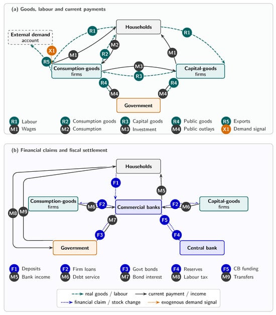
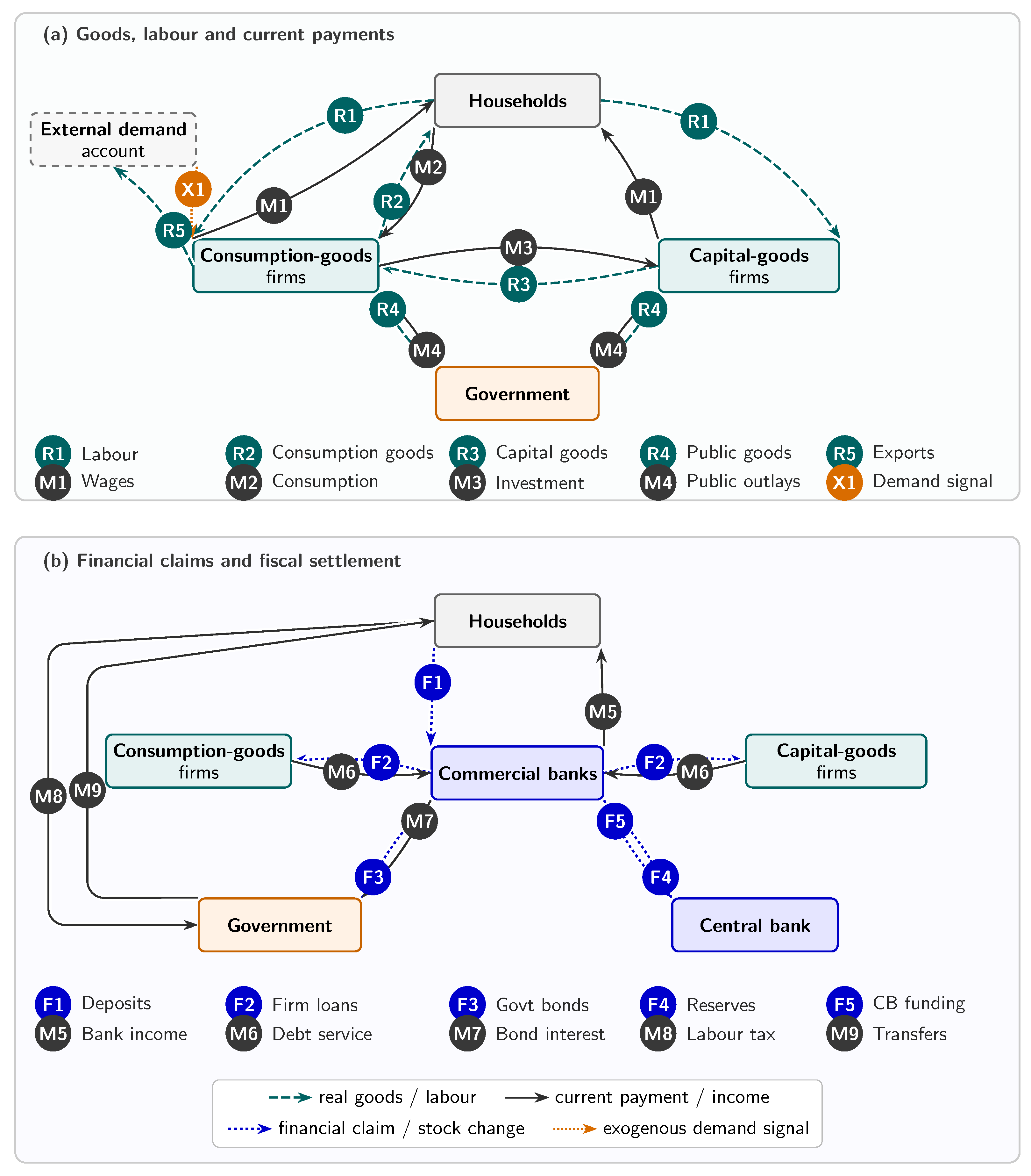
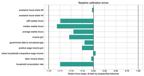
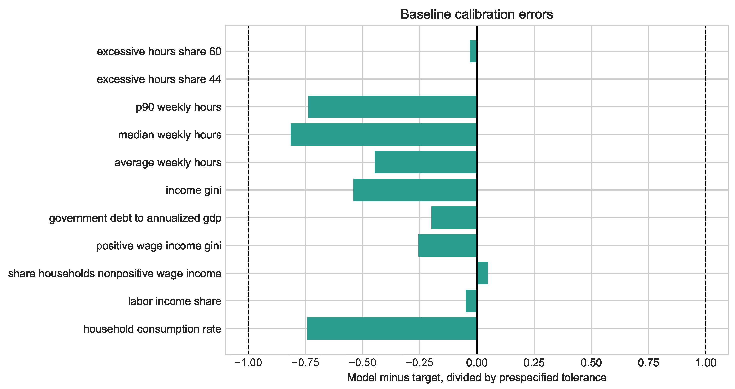
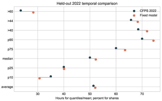
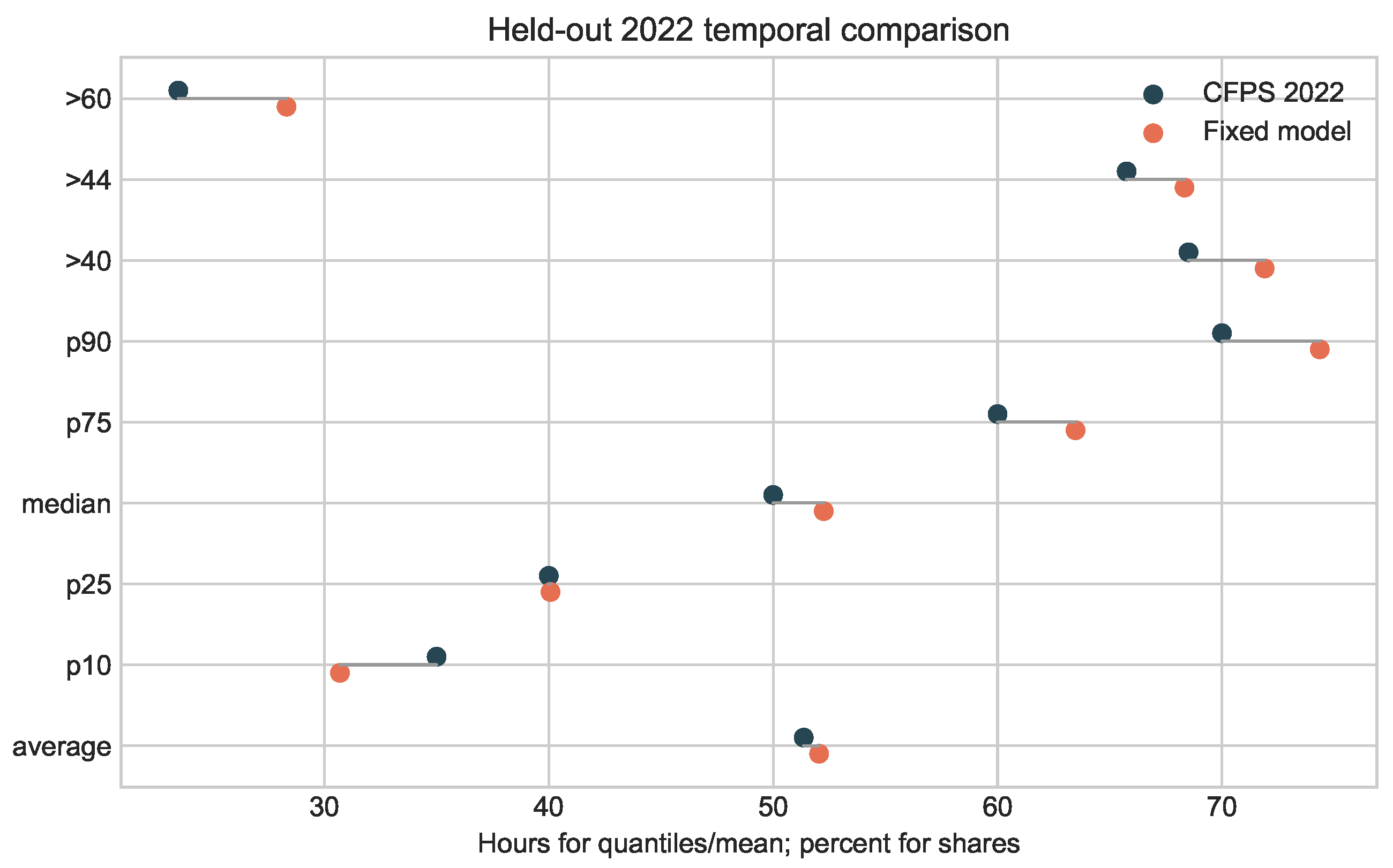
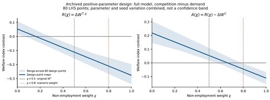
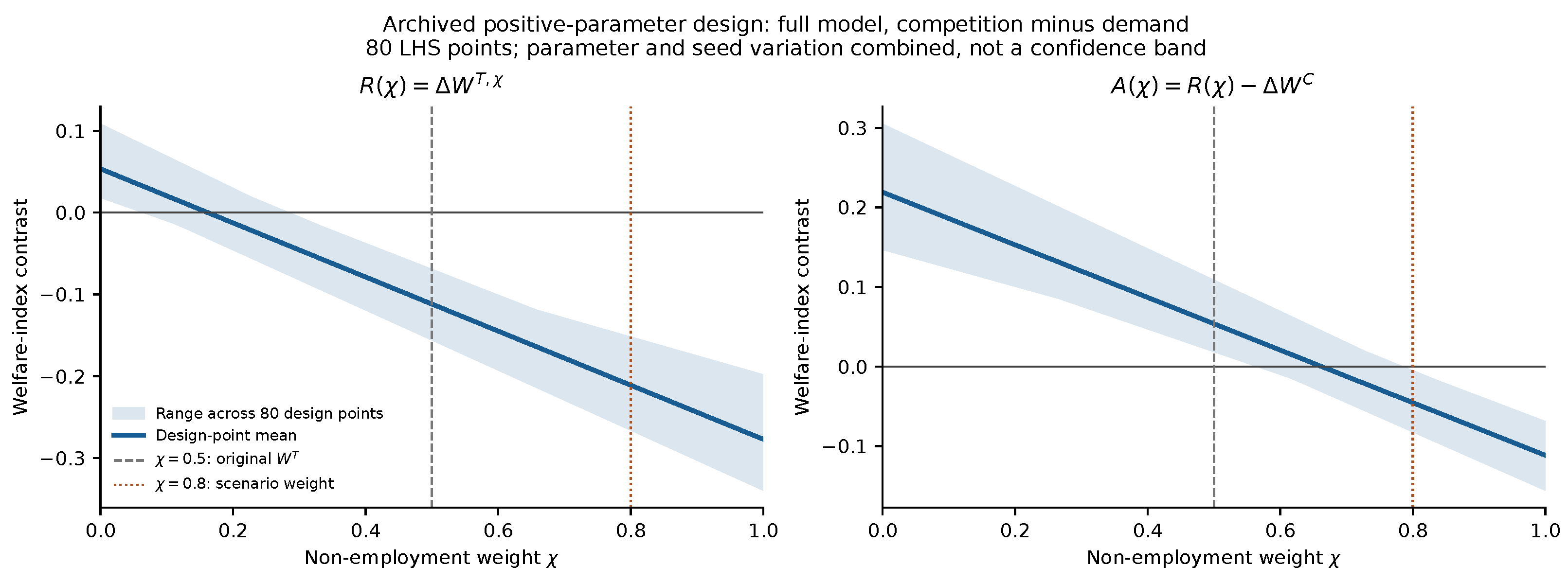
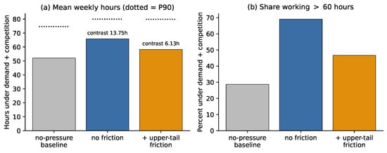
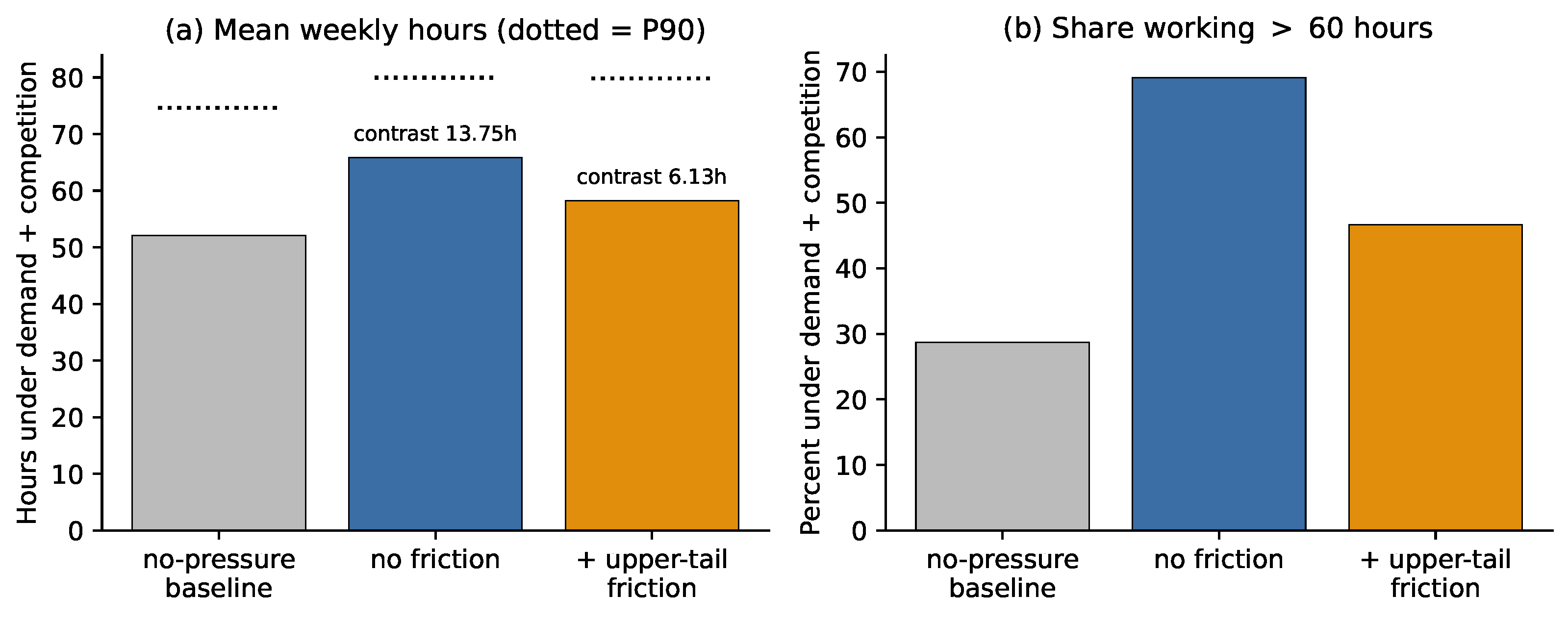
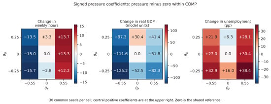
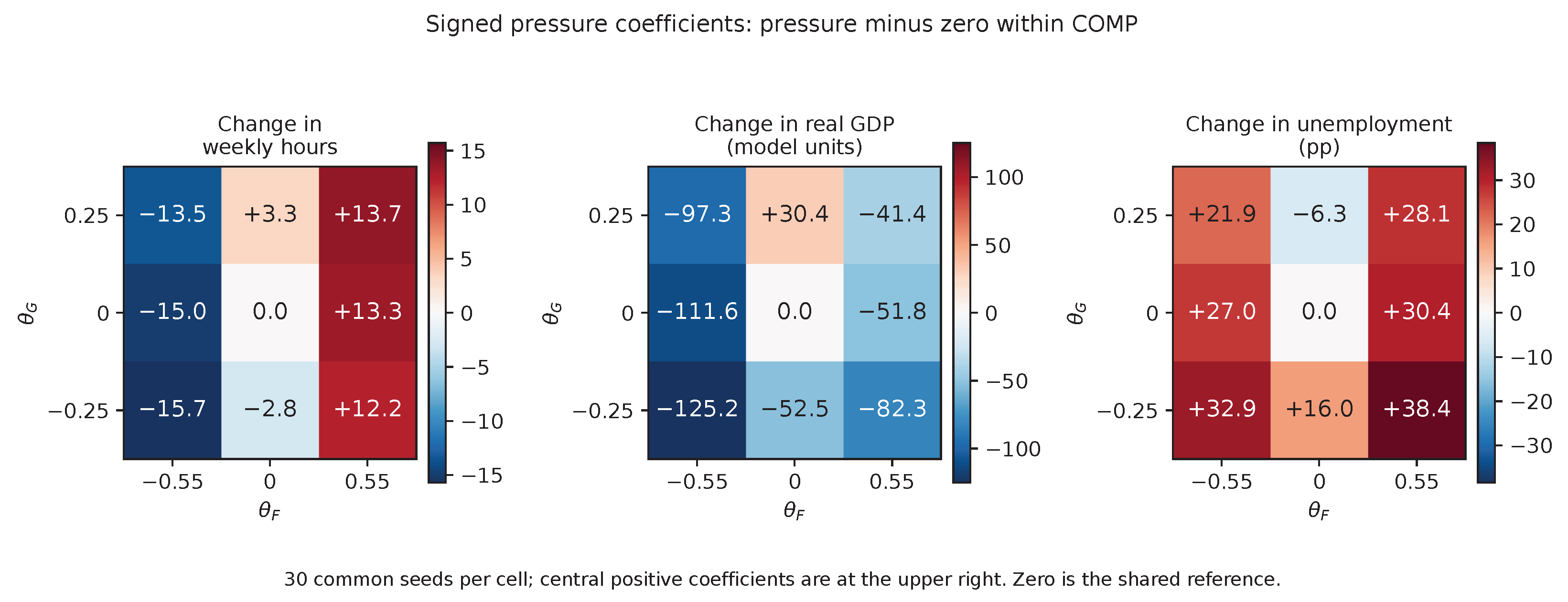
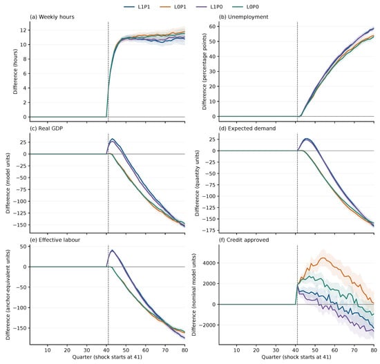
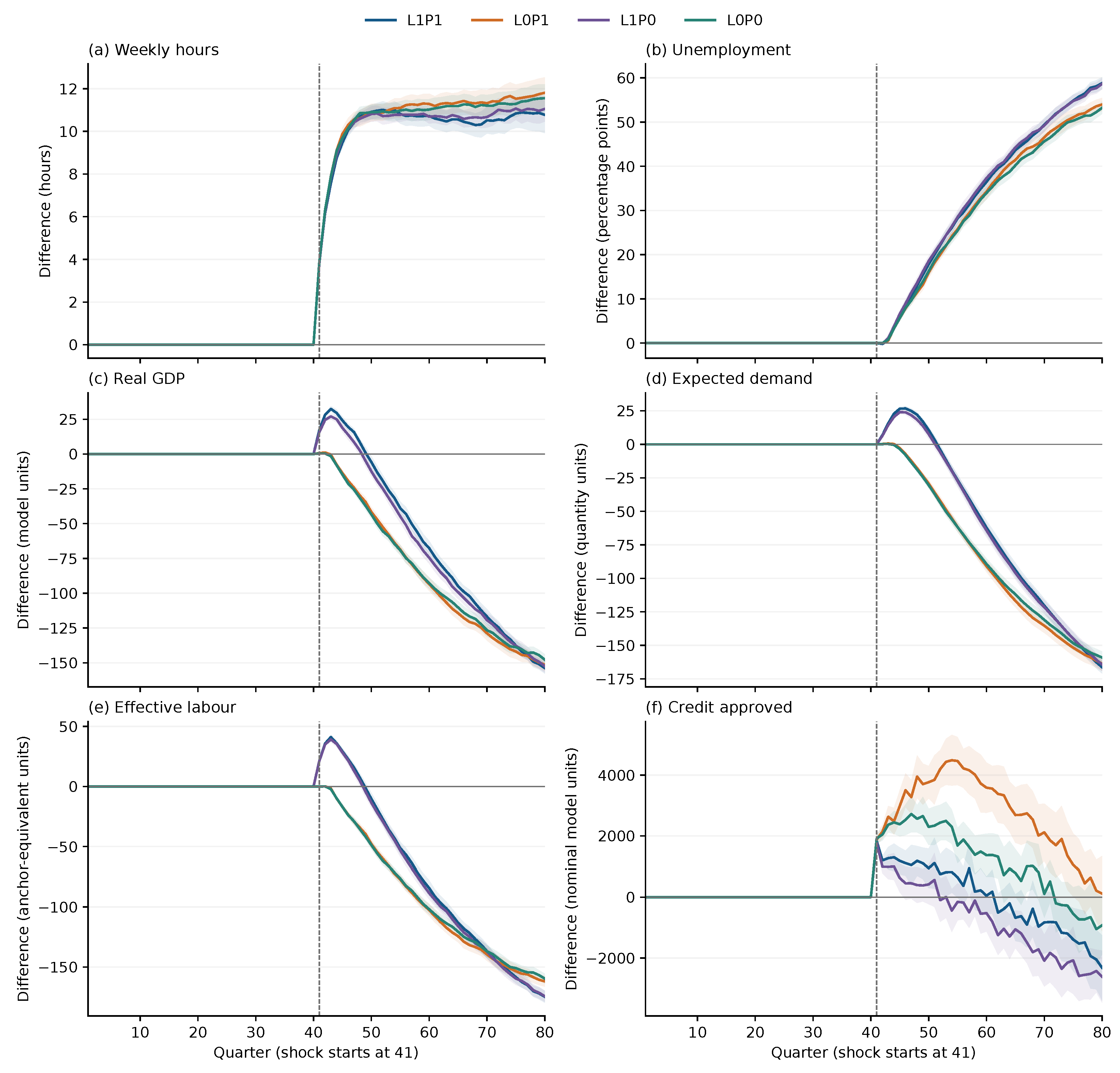

Disclaimer/Publisher’s Note: The statements, opinions and data contained in all publications are solely those of the individual author(s) and contributor(s) and not of MDPI and/or the editor(s). MDPI and/or the editor(s) disclaim responsibility for any injury to people or property resulting from any ideas, methods, instructions or products referred to in the content. |
© 2026 by the authors. Licensee MDPI, Basel, Switzerland. This article is an open access article distributed under the terms and conditions of the Creative Commons Attribution (CC BY) license.