Digital Twin Ready Predictive Risk Management of Subsurface Injection Nodes Using Mechanics Informed Cross Fault Machine Learning

Highlights

Please indicate how your work links to systems science via your contributions to systems practice, theory, and/or methodology.

• Frames the CCUS injection site as a local service node and defines a bounded advisory information contract that separates predictive risk, empirical domain support, operator judgment, and independent physical limits.
• Introduces a reproducible systems methodology combining a seven-variable state, source-only multi-horizon calibration, persistence rules, and a separate empirical support gate for cross-condition evaluation.

What are the main findings and/or the implications of the main findings?

• Watch and Mitigate intercepted all selected original-cohort target events in both transfer directions, but reverse transfer produced 22.9 and 42.2 s/event of early alert exposure, respectively.
• An independent specimen revealed policy-transfer failures despite 99.7–100.0% overall domain-support coverage, showing that domain similarity cannot replace prospective calibration, operator evaluation, or field validation.

Abstract

Predictive monitoring of injection operations requires evidence that warning rules transfer across fault conditions and loading rates. We develop a seven-variable representation of mechanical, hydraulic, and acoustic measurements and retrospectively evaluate source-calibrated Watch, Mitigate, and Hold indicators over 60, 30, and 10 s horizons. A separate Mahalanobis gate measures similarity to the source states. The original cohort comprises 18 pressure-stage events from two rough specimens and one smooth specimen; an independent archive adds six slow-creep stage peaks from a fourth specimen. A pump-based reconstruction reproduces every original event and model input. In the original rough-to-smooth transfer, Watch and Mitigate intercepted 6/6 events, with median warning time s of 16.5 and 3.5 s. In reverse transfer, both indicators intercepted 12/12 events but produced 22.9 and 42.2 s/event of pre-horizon alert activity. Deleting one smooth-source event changed support coverage in the final 30 s to 19.7–88.6%. On the independent specimen, the unchanged rough-source Watch indicator intercepted 5/6 peaks, whereas Mitigate and Hold intercepted none. The smooth-source Mitigate indicator intercepted 6/6 peaks but was active before its horizon for 72.8 s/event. Despite these contrasting outcomes, the source-domain gates included 99.7–100.0% of external states. The contributions are reproducible event construction, source-only policy evaluation, calibration sensitivity analysis, and an independent laboratory transfer test. The results show that high empirical support does not establish transferable warning thresholds. They motivate further advisory evaluation with separate prediction and support outputs. Four specimens, retrospective processing, and the absence of field validation do not establish operational readiness.

1. Introduction

Industrial decarbonization increasingly depends on systems in which physical assets, digital services, and operational decisions are tightly coupled. Carbon capture, utilization, and storage (CCUS) is one such system: carbon dioxide is captured at distributed sources, conditioned, transported through shared infrastructure, and delivered to utilization or geological storage nodes. Classical CCUS supply-chain optimization has focused on source–sink matching, transport topology, capacity expansion, cost, and storage uncertainty [1,2,3]. Recent resilience models additionally represent utilization or storage facilities as nodes that can lose capacity or become unavailable, requiring rerouting, redundancy, or transshipment [3]. These formulations motivate estimating the local condition of an injection node before declaring a loss of service capacity.

Digital twins (DTs) provide a natural architecture for this problem because they couple a physical asset to a digital representation that supports state estimation, forecasting, and decision support. The literature distinguishes static digital models, one-way digital shadows, and more complete twins by the degree and direction of data integration [4,5]. In supply chains, DTs are increasingly linked to disruption analytics, resilience, visibility, and real-time decision making [6,7,8,9,10]. Recent work in Systems similarly connects DT capability with logistics robustness and resilience, reinforcing the need to evaluate risk-management capability rather than digital representation alone [11]. Current reviews nevertheless show that many implementations remain conceptual or pilot scale, with continuing challenges in synchronization, interoperability, uncertainty, and trustworthy decision automation [7,8,9,10]. These limitations are particularly important for safety-critical assets, where a high prediction score is not by itself a sufficient basis for automated action.

Industry 5.0 emphasizes resilient, sustainable, and human-centered systems [12]. Here these principles motivate proposed design choices: expose uncertain predictions to operators, retain independent physical constraints, and examine unnecessary alert activity as well as missed events. They do not establish a digital twin maturity standard or imply that a laboratory predictor is ready for operational use. Effects on resilience, sustainability, operator performance, and carbon handling capacity are not measured in this study.

The physical challenge is that injection-related slip depends on stress, pressure, deformation, and fault properties. The source experiments show that fault roughness affects nucleation, localization, and macroscopic slip [13]. Laboratory and field studies document injection-associated aseismic and seismic motion, as well as conditions under which slip can stabilize [14,15,16,17,18,19]. Data-driven laboratory studies show that acoustic and mechanical signals can contain information about approaching failure [20]. Transfer to a different fault condition nevertheless requires checking how target trajectories relate to the source observations.

Recent subsurface DT research addresses rapid forecasting and uncertainty for geological carbon storage and geothermal operations [21,22]. The empirical scope of the present study is limited to retrospective fault-slip risk assessment using laboratory measurements. We evaluate horizon-specific indicators, alert activity within selected exposure windows, and a statistical domain support flag. An injection node is the intended future application; CCUS network planning provides context but lies outside the evaluated system boundary. We do not estimate injection capacity, network allocation, disruption propagation, or economic benefit.

The study uses the openly archived fluid injection experiments of Wang et al. [13,23], comprising two rough fault specimens and one smooth fault specimen under a six-stage pressure protocol. These data also underpin a separate geomechanics analysis by the authors [24]. The present study does not reuse that work’s 71-feature benchmark, recurrent network comparison, covariance alignment experiment, permutation controls, or SHAP ranking as primary results. It evaluates seven variables, source-calibrated alert policies, event-window alert exposure, and domain support. Shared experimental data and preprocessing are disclosed; the distinct endpoint is the behavior and limitations of these retrospective decision-support indicators. The revision additionally tests the unchanged source policies on a separately archived slow-pressurization specimen [25,26]; this external cohort is evaluated separately and is not used to refit or tune the original models.

Four research questions guide the work:

RQ1: Can the archived hydraulic, stress, deformation, velocity, and acoustic measurements be represented by seven physically interpretable variables for retrospective fault-slip risk assessment?

RQ2: How do horizon-specific Watch, Mitigate, and Hold indicators compare with hydraulic-only and acoustic-only reference policies in event interception, warning time, and alert exposure under source-only calibration?

RQ3: How sensitive are empirical domain support estimates to the source events, cutoff, temporal sampling, and distance formulation?

RQ4: What local advisory interface can distinguish predicted urgency from empirical support, and which parts remain conceptual until prospective validation?

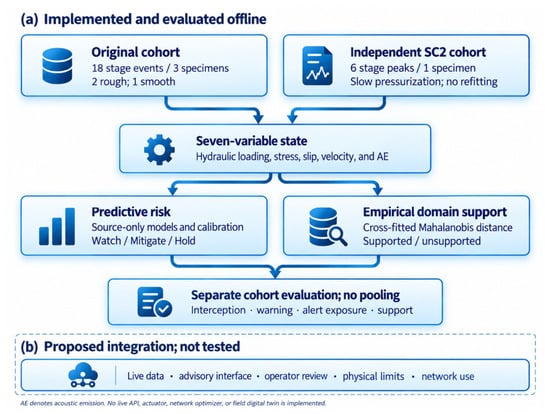
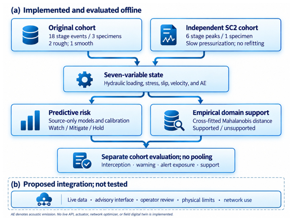
The empirical contributions are a seven-variable representation, source-only calibration of three persistent risk indicators, a separate source-distance gate, and an evaluation that reports event counts, warning times, alert exposure, support coverage, and sensitivity. A proposed local interface organizes the outputs for operator review; its controls and any connection to a CCUS network remain conceptual. The present artifact is an offline analytical prototype. It is neither a live digital shadow, which would require automatic one-way data updates, nor a deployed digital twin with operational feedback [4,5]. Operational maturity is therefore not claimed. Figure 1 summarizes the evaluated study boundary and distinguishes the implemented offline analysis from the proposed, untested integration pathway.

Figure 1. Study boundary and proposed integration. (a) The implemented offline workflow constructs the seven-variable state and evaluates source-calibrated risk indicators and empirical domain support. The original 18-event, three-specimen cohort and the external six-peak SC2 cohort are evaluated separately. (b) Live data connection, the advisory interface, operator review, independent physical constraints, and CCUS network use remain proposed. AE denotes acoustic emission. No live API, actuator, network optimizer, or field digital twin is implemented.

2. Conceptual and Systems Framework

2.1. The Injection Node as a Supply-Chain Service Node

An injection site receives CO₂ subject to pressure, injectivity, containment, and regulatory constraints. A reduction in admissible capacity could require upstream buffering, rerouting, or curtailment; network models represent such changes as facility disruptions [1,2,3]. Laboratory slip measurements do not directly determine that capacity. This study investigates local risk indicators that could eventually inform site assessment, without calculating service loss or network response.

The proposed local interface is {risk tier, support flag, advisory action class, timestamp, data quality flag}. The risk tier is Normal, Watch, Mitigate, or Hold. It summarizes the horizon-specific persistent alarms, with Hold taking priority over Mitigate and Watch in the display. The support flag is separate: “unsupported” means that the seven-variable state has a Mahalanobis distance greater than the chosen source cutoff. This flag indicates insufficient empirical similarity to the training conditions; it does not establish impending failure, sensor malfunction, or safety. A “supported” flag does not certify safety either. Timestamps and data quality checks are deployment requirements, not evaluated live services.

2.2. Advisory Actions and Industry 5.0 Design Principles

An advisory action class is a proposed categorical workflow label, not a quantity learned from the data or a calculated permission to control injection. The classes are routine monitoring (Normal), enhanced monitoring (Watch), operator assessment of a possible rate modification (Mitigate), operator assessment of a possible interruption (Hold), and review required when the support flag is unsupported. A detailed version of this proposed mapping is presented in Section 4.5. All classes remain advisory in this study. The interface cannot authorize a change in pressure or rate, and an unsupported flag must never suppress independent alarms or approved safety limits.

Industry 5.0 provides a rationale for this proposed separation of information and authority [12]. Resilience motivates displaying emerging risk and limitations; sustainability motivates investigating both missed events and unnecessary alert activity; human-centered operation motivates operator review. These are design intentions, not demonstrated outcomes or requirements for a certified “readiness” level. Live synchronization, prospective calibration, independent specimens, operator testing, and a validated physical operating envelope would be needed before considering operational integration.

2.3. Design Requirements

Table 1 summarizes the design requirements, their rationale, and the corresponding implementation status of the retrospective prototype.

Table 1. Requirements and intended design elements of the retrospective risk assessment prototype.

ID	Requirement	Rationale	Implementation
DR1	Traceable compact state	Use defined measured quantities and document temporal availability.	Seven variables; retrospective interpolation adds <0.100 s availability delay.
DR2	Horizon-specific indicators	Describe different warning windows without authorizing controls.	Watch 60 s, Mitigate 30 s, Hold 10 s; all advisory.
DR3	Source-calibrated settings	Keep target outcomes out of threshold fitting.	Source OOF negative quantiles; explicit persistence sensitivity.
DR4	Empirical support diagnostic	Report distance and its calibration dependence.	Cross-fitted Mahalanobis gate and alternative sensitivity checks.
DR5	Operator and physical limits	Separate analytics from operational permission.	Conceptual review mapping only; no actuation tested.
DR6	Reproducible analysis	Supply inputs, code, exact settings and provenance.	Versioned files and audits; public revision repository pending.
DR7	Local advisory interface	Expose local risk and support separately.	Proposed tuple; live and network integration unimplemented.

3. Materials and Methods

3.1. Design Science Research Logic

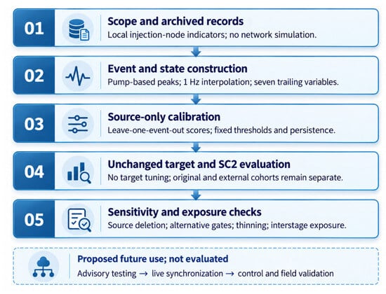
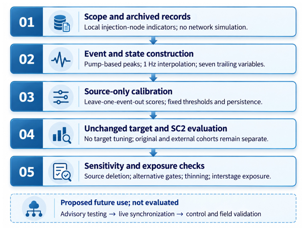
The study follows a design science approach: it constructs an analytical artifact, evaluates its measurable components, and distinguishes those results from proposed operational uses [27,28]. Figure 2 summarizes the workflow. The empirical analysis covers feature representation, source-only policy calibration, retrospective alert metrics, and statistical support diagnostics. Human review, physical fallback, and network integration are conceptual extensions, not empirically verified capabilities.

Figure 2. Retrospective workflow from archived records to source-only calibration, unchanged target and SC2 evaluation, and sensitivity and interstage-exposure checks. The numbered stages are implemented offline. The dashed box identifies proposed future advisory, live-synchronization, control, and field-validation work, not an evaluated control loop.

3.2. Experimental Data and Analytical Unit

This study presents a secondary analysis of the public dataset released by Wang [23] and described experimentally by Wang et al. [13]. Three cylindrical Bentheim sandstone specimens (50 mm in diameter and 100 mm in length) contained faults inclined at 30° to the specimen axis. Two interfaces were produced by shear fracture and had reported root-mean-square (RMS) surface heights of 1.50 and 0.82 mm. The smooth interface was saw-cut and polished, with an RMS height of 0.044 mm. The specimens were held at a confining pressure of 35 MPa and an initial pore pressure of 5 MPa, then subjected to six 10 min injection stages that increased pore pressure from approximately 5 to 29 MPa. Each stage consisted of an approximately 4 MPa ramp followed by a plateau [13].

The archive contains hydraulic, stress, slip, velocity, and processed AE channels sampled at approximately 10 Hz. An audit against the original workbooks shows that the supplied 1 Hz histories were produced by linear interpolation onto a specimen-specific regular grid, rather than by within-second averaging. The next raw bracketing observation can occur up to 0.100 s after the grid timestamp. The analysis is therefore retrospective; strict zero-latency online causality is not demonstrated. Eighteen previously fixed stage events are retained, six per specimen. Each predictor window contains exactly 180 rows with lead ℓ = 180, …, 1 s before the catalog peak; the peak row at ℓ = 0 is excluded.

For the revision, physical injection ramps are detected from the raw records after interpolation to the existing 1 Hz grid. A trailing five-sample mean pump rate must exceed 0.1 mL/min for at least five consecutive samples. The first sample of each qualifying run defines its ramp start. Each event peak is the earliest maximum slip velocity from that start to the sample before the next ramp start; the final search ends with the record. This automatic reconstruction adds or removes no event and reproduces all 18 frozen peaks. At a fixed five-sample mean, all nine combinations of pump thresholds 0.05, 0.10 and 0.20 mL/min and run lengths 3, 5 and 10 s recover the same peaks from both raw-reconstructed and archived cleaned inputs.

The archived injection_stage boundaries are midpoint partitions between successive selected peaks, not physical ramp onsets. They are not inputs to the new reconstruction. Historical annotation decisions remain undocumented. The current explicit algorithm was developed during revision with the catalog available and is not an independent validation exercise. Secondary local velocity fluctuations are not counted as additional events. The reconstruction reproduces all 3240 labels and the seven-variable model inputs, with a maximum absolute feature error below 1.5 × 10⁻¹¹. Supplementary Table S2 and the executable raw-to-event reconstruction specify every search interval, selected peak, and feature window.

For horizon h, the label is y_h(t) = 1 when 0 < ℓ(t) ≤ h and 0 otherwise. Thus, each 180-row event has 60, 30, or 10 positive rows at the three horizons. Selection is conditional on a future catalog peak and enriches the sample with observations preceding slip; it does not reproduce the prevalence encountered during continuous surveillance. Long interstage periods were excluded from the original event-centered comparison to standardize its exposure window. Consequently, that comparison cannot estimate false alarms during quiet periods. The revision evaluates archived interstage exposure separately in Section 3.9.

Successive stages share a specimen, fault surface, and pressure history. Events are therefore repeated observations rather than independent experimental replicates. The source and target specimen groups are disjoint for each transfer direction, but event-based source cross validation still shares specimen history across its training and omitted event folds. Table 2 summarizes the three original-cohort specimens, their fault-surface characteristics, sampling rates, and event counts.

Table 2. Original-cohort experimental data used to evaluate the node-level predictive risk artifact. The independent SC2 cohort is described in Section 3.10.

Specimen	Fault Surface	RMS Height (mm)	Archived Sampling (Hz)	Events
Rough fault 1	Shear fractured	1.50	~10.30	6
Rough fault 2	Shear fractured	0.82	~10.16	6
Smooth fault	Saw cut/polished	0.044	~10.04	6

Note: Three specimens provide six pressure-stage events each. These are repeated observations within specimens, not 18 independent specimens. Experimental configuration and roughness follow Wang et al. [13], and the time series are archived in [23].

3.3. Compact Digital State

The companion study [24] used a broad predictor set. The present analysis selects seven variables to summarize measured forcing and fault response. “Mechanics-informed” means that these engineered quantities have physical interpretations; it does not mean that the logistic model enforces governing mechanical equations. Equation (1) is the authors’ chosen state definition, not a new constitutive law:

$$z(t)={[r_H,{\dot{p}}_{30},{\Delta \tau }_{30},{\Delta {\mathit{\sigma }}^{\prime }}_{n,30},{\Delta \mathsf{\delta }}_{30},{\overline{v}}_{30},\mathit{log}[1 + {A\overline{E}}_{30}] ]}^T$$

(1)

All components in Equation (1) are evaluated at t. Here r_H = p/(p + σ′_n) is pore pressure divided by resolved total normal stress under the archived stress convention. At each 1 Hz row, the pressure change rate is [p(t) − p(t − 29 s)]/29 s. The shear stress, effective normal stress, and slip increments are likewise current values minus values 29 s earlier. Mean velocity uses the available samples from t − 29 s through t, with a minimum of 24 of the 30 rows; the same availability rule applies before transforming the mean AE rate. The raw-record audit confirms that every reported event window actually has all 30 samples available for these means. The acoustic variable is log [1 + mean AE rate over those same 30 samples], with the numerical rate expressed in the archived counts-per-second units. Thus “30 s” in the feature labels denotes 30 sampled values spanning 29 s, not a fitted pressure trend or a 30 s endpoint difference. These definitions reproduce all 3240 rows of the supplied seven-variable matrix. They are trailing quantities on an interpolated retrospective stream; its subsecond availability limitation is described in Section 3.2. Table 3 summarizes the seven state variables, their operational interpretations, and their sensor or physics families.

Table 3. Seven physically interpretable variables used in the retrospective analysis.

State Variable	Operational Meaning	Sensor/Physics Family
Hydraulic loading ratio, rH	Pore pressure fraction of resolved total normal stress: p/(p + σ′n)	Hydraulic
30 s pressure slope, $\dot{p}$30	Endpoint pressure difference divided by 29 s	Hydraulic
30 s shear stress change, Δτ30	Stress redistribution/weakening	Mechanical
30 s effective normal stress change, Δσ′n,30	Effective stress evolution	Mechanical
30 s slip increment, Δδ30	Preslip accumulation	Deformation
30 s mean slip velocity, $\overline{v}$30	Incipient kinematic acceleration	Kinematic
Log mean AE rate, log(1 + ĀE30)	Log transform after averaging the 30 sampled AE rates	Acoustic

3.4. Source Domain Probabilistic State Estimators

Three laboratory forecast horizons are considered: 60 s for Watch, 30 s for Mitigate, and 10 s for Hold. This ordering separates early awareness from warnings progressively closer to the peak; these durations are not validated field response times. The logistic estimator uses RobustScaler with the 10th to 90th percentile range, C = 0.5, balanced class weights, the liblinear solver, and a maximum of 3000 iterations. Equation (2) uses the standard logistic link presented by James et al. [29] with a source-only additive log-odds correction, c_h. This correction targets calibration-in-the-large using source out-of-fold scores [30]; it does not establish a unit calibration slope, target probability calibration, or the correctness of individual predictions. Here $\tilde{z}$(t) denotes the source-scaled state, β denotes the fitted logistic coefficients, and c_h denotes the additive source correction.

$$P_h(t)={[1+\mathit{exp}(-({\beta }_{0,h}+{\beta }_h^T \tilde{z}(t)+c_h)\left)\right]}^{-1}$$

(2)

A domain is a specified specimen group with a common fault surface category. For rough-to-smooth transfer, the source contains 12 events from the two rough specimens and the target contains six events from the smooth specimen. For smooth-to-rough transfer, these roles reverse. Target labels are used only for retrospective evaluation. In each source domain, leave-one-event-out fitting produces scores for the omitted event; the scaler is fitted within each fold. An additive intercept correction is estimated from those source scores, followed by a final fit on all source events and application of the same correction to the target. Other events from the same specimen can remain in an event fold, so this procedure does not establish generalization to independent specimens [31]. The intercept correction itself uses all source out-of-fold labels; it is a source calibration step, not an independently nested assessment of calibration quality.

3.5. Source-Calibrated Risk Tiers

Equation (3) is the authors’ empirical policy threshold definition, using a standard sample quantile operation. Let P_h^OOF denote source out-of-fold probabilities after the intercept correction and y_h = 0 denote seconds outside the selected slip horizon. The threshold is

$$T_h=Q_q\{ P_h^{\mathit{OOF}}(t) \mid y_h(t)=0 \}$$

(3)

Watch uses the 0.90 quantile of source-negative scores and 5 s persistence; Mitigate uses 0.95 and 3 s; Hold uses 0.99 and 2 s. These are illustrative policy settings, not uniquely optimal or experimentally established constants. Increasing the quantile requires more extreme scores for more consequential labels. Approximately 10%, 5%, and 1% of source-negative scores lie above the respective cutoffs before persistence is applied, subject to ties. These proportions are neither target false-alarm probabilities nor event probabilities. Shorter persistence at shorter horizons limits the delay relative to the available warning period. These exact settings have not been justified by an optimization of cost, response time, or safety. We therefore report sensitivity results rather than present the settings as universal choices. Table 4 summarizes the three risk tiers and the two reference policies, including their horizons, source-negative quantiles, persistence settings, and intended roles.

Table 4. Risk tiers and reference policies.

Policy	Horizon (s)	Source-Negative Quantile	Persistence (s)	Intended Role
Watch	60	0.90	5	Advisory enhanced monitoring
Mitigate	30	0.95	3	Advisory operator rate review
Hold	10	0.99	2	Advisory interruption review; unvalidated
Hydraulic-only baseline	30	0.95	3	Reference policy from rH, pressure slope, pump mean
Acoustic-only baseline	30	0.95	3	Reference policy from AE level/history

Note: Settings are calibrated using source data. At each second, the indicator becomes active only after the required number of consecutive scores at or above the threshold. It resets when the score falls below the threshold; activation is not latched until the event. Source-negative fractions describe only the selected event windows.

In the revision sensitivity analysis, each horizon model was evaluated at q ∈ {0.90, 0.95, 0.99} and persistence ∈ {1, 2, 3, 5} s in both directions, giving 72 configurations. Thresholds always use source scores, and no target outcome was used to select a replacement setting. This is an exploratory post-review analysis. Exact thresholds and all outcomes appear in Supplementary Tables S1 and S4 and the accompanying CSV files.

3.6. Reference Policies

Two 30 s reference policies use the same 0.95 source-negative quantile and 3 s persistence as Mitigate. The hydraulic policy uses the hydraulic loading ratio, pressure change rate, and mean pump rate. The acoustic policy uses the log-transformed instantaneous AE rate, mean AE rate, and AE burstiness. These policies provide comparisons under a common calibration rule; they are not optimized single-sensor benchmarks. Comparisons across horizons also reflect differences in label prevalence.

3.7. Domain Support Gate and Support-Eligible Coverage

The support gate summarizes distance from source experience independently of predicted slip probability. For each omitted source event, robust scaling and Ledoit–Wolf shrinkage covariance [32] are fitted to the remaining source events, and the omitted event distances are recorded. The pooled 99th percentile is retained as an illustrative reference cutoff, alongside 95th, 97.5th, and 99.5th percentile alternatives. The final scaler and covariance are fitted to all source events and applied to the target specimen group defined in Section 3.4. Equation (4) uses the standard Mahalanobis-distance form discussed by Cabana et al. [33], with the Ledoit–Wolf covariance estimate used here [32]; it is not a new distance proposed in this study:

$$D(t) = \sqrt{{\left[z_s\right(t) - {\mu }_s]}^T {\mathit{\Sigma }}_s^{-1} [z_s(t) - {\mu }_s]}$$

(4)

Here z_s(t) is the target state after source scaling, μ_s is the fitted source mean, and Σ_s is the shrinkage covariance. A second is flagged unsupported if D(t) > D_crit. The reference quantile has a nominal 1% exceedance interpretation in the cross-fitted source sample only. There is no distribution-free 99% guarantee for future events, specimens, or target data, especially because rows are autocorrelated and the final fit differs from the cross-fitting models. The 99th percentile is not claimed to be a validated safety cutoff or an independently preregistered optimum. Equation (5) is the authors’ empirical summary of the fraction of evaluated seconds inside the chosen envelope:

$$A_H = {\displaystyle \frac{1}{N_H}} {\mathit{\Sigma }}_{t\in H} I[D(t) \le D_{\mathit{crit}}]$$

(5)

A_H denotes support coverage within the specified evaluation window H, N_H is the number of one-second rows in that window, and I[·] is the indicator function. The gate measures similarity in the chosen coordinates and covariance geometry. It provides neither a calibrated probability that a prediction is correct nor a test of physical admissibility. Unsupported observations warrant review in the proposed interface, while independent physical constraints remain applicable regardless of the flag.

Additional support diagnostics use source and target distance distributions, each omitted event’s q99, full recalibration after deleting one source event, and source thinning at 5, 10, and 30 s. Alternatives are a diagonal robust distance and an RBF one-class SVM with gamma = scale and nu = 0.01 [34], each using source-only cross-fitted q99 calibration. A two-fold whole-rough-specimen calibration is also evaluated; no whole-smooth-specimen calibration is possible with one specimen. These are sensitivity analyses, not new independent validation data.

To describe the score, let δ = z_s − μ_s and P = Σ_s⁻¹. The signed coordinate contributions c_j = δ_j(Pδ)_j sum exactly to D². Because the coordinates are correlated, contributions can be negative. They are neither independent percentages nor measures of causal importance. Source-distance distributions, event cutoffs, coordinate contributions, and all recalibration results are provided in Supplementary Section S5.

3.8. Evaluation Metrics and Decision Logic

Event interception is the fraction of target events with a persistent alarm at a lead time 0 < ℓ ≤ h. Warning time is the largest qualifying lead within that horizon and is summarized as the median among intercepted events; it provides no warning estimate for missed events. Pre-horizon intervention burden is the mean number of active seconds with ℓ > h per selected event. For example, 42.2 s/event means that the indicator was active for that average duration before its 30 s horizon within the available 180 s window. Larger values indicate more early alert exposure within that window. Whether such exposure is beneficial or unnecessary depends on an untested response policy. Intervention duty fraction is the fraction of all target-window seconds with an active indicator. These are alert metrics: no intervention was performed, and the metrics do not estimate throughput loss, field false-alarm rates, or the burden over months of quiet operation. The policy metrics are ungated: the support flag is reported separately and does not suppress alarms in the calculation of Table 5.

Table 5. Original-cohort retrospective policy performance within 180 s event windows. Interception includes observed counts; AP denotes average precision. Burden and duty measure indicator activity only and do not represent false alarms over months of quiet operation, performed interventions, or CO₂ throughput losses. Hold is an evaluated diagnostic indicator, not a validated control policy.

Direction	Policy	h (s)	AP	Intercept n/N (%)	Median Warning (s)	Pre-Horizon Burden (s/Event)	Duty (%)
Rough → Smooth	Hydraulic-only	30	0.77	5/6 (83.3)	3.0	0.0	1.2
Rough → Smooth	Acoustic-only	30	0.66	5/6 (83.3)	7.0	0.0	5.2
Rough → Smooth	Watch	60	0.98	6/6 (100.0)	16.5	0.0	9.5
Rough → Smooth	Mitigate	30	0.81	6/6 (100.0)	3.5	0.0	2.7
Rough → Smooth	Hold	10	0.57	1/6 (16.7)	1.0	0.0	0.1
Smooth → Rough	Hydraulic-only	30	0.74	11/12 (91.7)	30.0	30.8	31.7
Smooth → Rough	Acoustic-only	30	0.53	8/12 (66.7)	30.0	6.0	11.1
Smooth → Rough	Watch	60	0.97	12/12 (100.0)	60.0	22.9	45.7
Smooth → Rough	Mitigate	30	0.89	12/12 (100.0)	30.0	42.2	40.1
Smooth → Rough	Hold	10	0.53	10/12 (83.3)	10.0	26.0	19.1

Precision–recall discrimination is calculated using average_precision_score, referred to as average precision (AP), rather than trapezoidal curve integration [35]. The positive fractions are 60/180, 30/180, and 10/180 for the respective horizons in both transfer directions. Brier score measures mean squared probability error [36]; general calibration concerns are discussed in [30,37]. Wilson score intervals for a binomial proportion [38] and 10,000 event-bootstrap resamples are retained as descriptive summaries conditional on the observed specimens. They do not correct dependence between stages within a specimen or quantify between-specimen uncertainty. Six and twelve events provide coarse interception increments of 16.7 and 8.3 percentage points. AP and Brier scores are displayed to two decimal places; rounding does not reduce statistical uncertainty. All proposed operational actions remain advisory.

3.9. Additional Archived Interstage Exposure

The revision evaluates continuous target intervals outside [catalog peak—180 s, catalog post-event end +30 s], requiring 30 consecutive finite samples for every state channel. These are archived interstage locked periods with low pump rate, not independently certified event-free periods. The original source models, intercept corrections, thresholds, persistence rules, and support cutoff remain frozen. Persistence is evaluated over all valid observations; exposure metrics count only eligible intervals, and excluded gaps separate counted alert episodes. We count active seconds and distinct alert episodes in eligible exposure; this is an additional retrospective laboratory diagnostic, not field false-alarm validation. Sensitivity uses 0, 30, and 60 s post-event buffers. Reconstructed event-window features and predictions were checked against the archived inputs and outputs before applying the models outside those windows.

Because the archived post-event end annotations have undocumented historical provenance, an additional analysis excludes a fixed interval from peak minus 180 s through peak plus 180, 210 or 240 s. It also requires complete feature histories and pump rate at or below 0.1 mL/min. This calculation uses no annotated event-end boundary and changes only the evaluation exposure; all model and policy parameters remain frozen. The fixed durations are sensitivity settings, not demonstrated times of physical recovery.

3.10. Independent Laboratory Transfer Evaluation

A separate published archive [25,26] contains two polished Bentheim specimens subjected to different pressurization rates. SC1 was excluded because its AE history matches that of the smooth specimen already used in this study across 39,500 shared timestamps (maximum rate discrepancy below 5.2 × 10⁻¹³ counts/s). Minor reprocessing of the channels does not make the specimen independent. SC2, pressurized at 0.5 MPa/min, provides one additional specimen and six pressure-stage slow-creep velocity peaks. It is evaluated separately from the original three-specimen cohort.

Channel-specific records are interpolated onto a common 1 Hz grid without endpoint extrapolation. Pump pressure is converted from bar to MPa. Archived effective normal stress is used directly; slip is expressed in mm, velocity in mm/s, and processed AE rate in counts/s. The six physical stages begin at the first pressure crossings of 5.10, 9.10, 13.10, 17.10, 21.10, and 25.10 MPa, following the published 4 MPa increments. The earliest velocity maximum in each interval defines its peak. All six windows have a complete 209-row history, do not overlap, and contain no earlier cataloged stage maximum within the 180 s preceding the peak. These are stage-wise slow-creep peaks, not six independent earthquakes.

Both original source models and their intercept corrections, quantiles, persistence rules, and support cutoffs are retained unchanged. External outcomes are not used to select events, a preferred source model, or a new threshold. Eligibility and unit checks were completed before predictions were computed. The evaluation reports all six peaks and all three indicators for both models; the results remain descriptive for one external specimen. The archived velocity and AE processing methods, together with sensor conventions, limit claims of exact measurement equivalence and online causality. Supplementary Section S11 documents the cohort, outcomes, duplication audit, and excluded candidate datasets.

4. Results

4.1. Risk-State Discrimination Using the Compact State

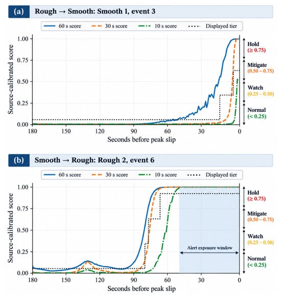
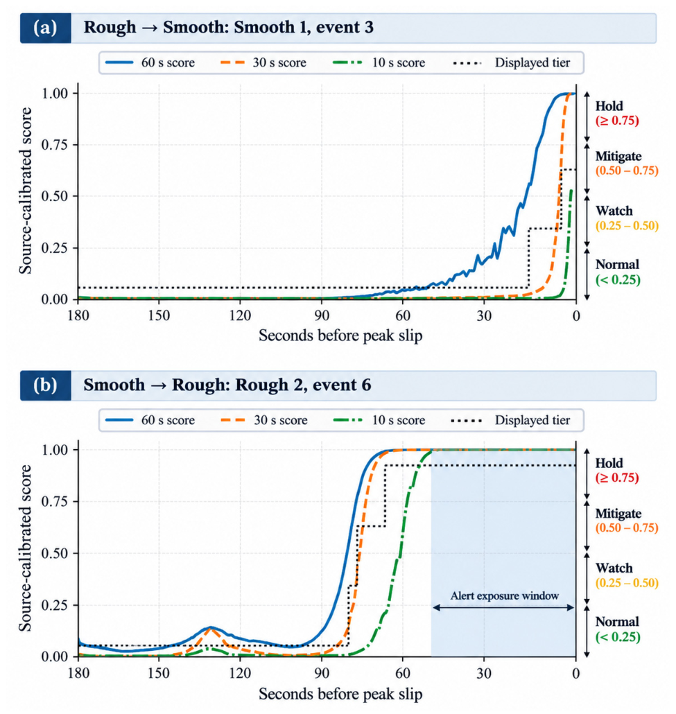
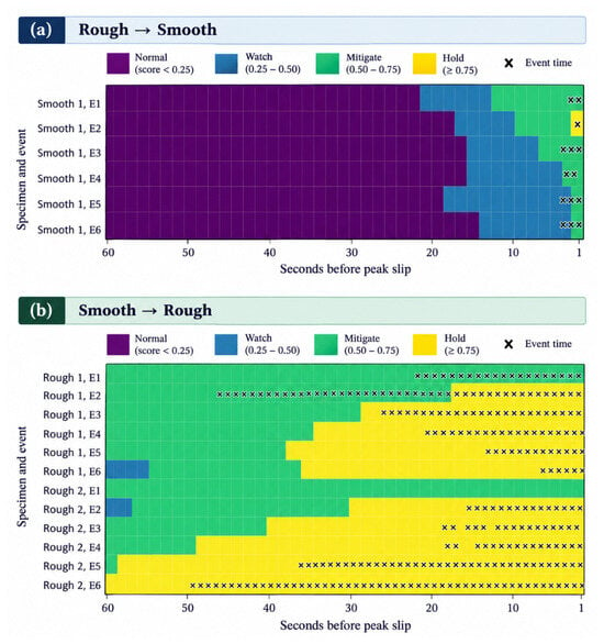
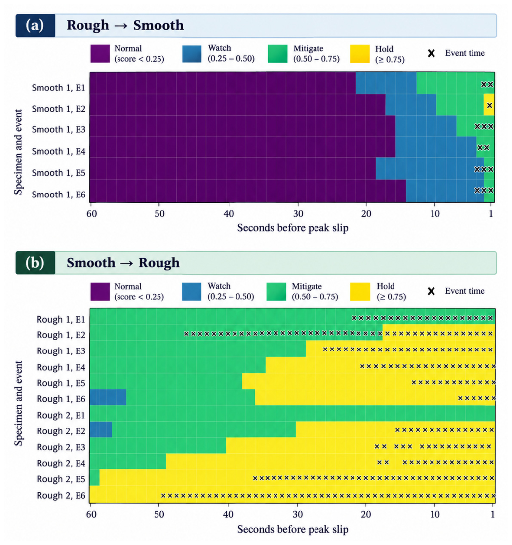
The seven-variable models showed retrospective discrimination in the selected windows. In rough-to-smooth transfer, AP was 0.98, 0.81, and 0.57 for Watch, Mitigate, and Hold, respectively; the reverse-transfer values were 0.97, 0.89, and 0.53. The monotonic intercept correction does not alter score ordering. These point estimates establish neither the superiority of one transfer direction nor performance in a broader population. Comparisons across horizons also involve different positive-label fractions, so the lower Hold AP alone cannot establish a physical cause of reduced performance. The limited 10 s interception evidence is evaluated separately in Table 5. Figure 3 illustrates representative source-calibrated score trajectories for both transfer directions, while Figure 4 summarizes the event-aligned risk tiers across all original-cohort target events.

Figure 3. Representative retrospective risk trajectories: (a) rough-to-smooth transfer for Smooth 1, event 3; (b) smooth-to-rough transfer for Rough 2, event 6. The left axis shows the source-calibrated 60, 30, and 10 s scores; the dotted stepped line uses the separate right-hand advisory-tier axis. Shading identifies seconds beyond the source-derived domain-support cutoff. Lead time decreases toward the peak. Scores and support answer different questions; neither authorizes an operational action.

Figure 4. Event-aligned risk tiers over the final 60 s: (a) the six smooth-target stage events; (b) the twelve rough-target stage events. The four discrete states share one legend, and crosses mark seconds beyond the source-derived support cutoff. The horizontal axis decreases toward the peak; each row is one stage event. Events from the same specimen are repeated observations, not independent experimental replicates. These maps do not represent implemented controls.

4.2. Policy-Level Trade-Off: Interception Versus Intervention Burden

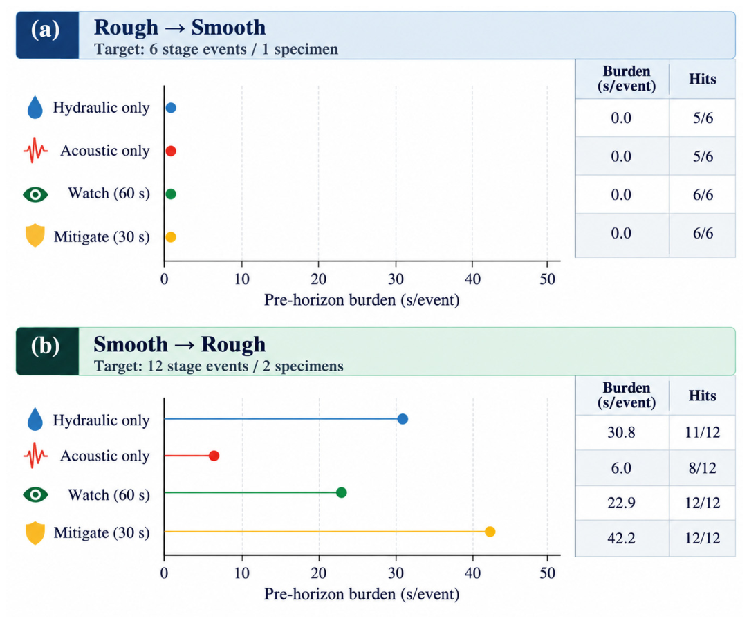
Table 5 reports observed counts as well as percentages. In rough-to-smooth transfer, Watch and Mitigate intercepted 6/6 events, with median warning times of 16.5 and 3.5 s and no pre-horizon alert activity in the selected windows. The nominal Wilson event-count interval for 6/6 is 61.0–100.0%; this wide interval does not establish reliable population detection and does not account for within-specimen dependence. Event-bootstrap intervals for the median warning times are 15.0–20.0 and 1.0–10.0 s, conditional on the observed smooth specimen. The hydraulic and acoustic policies each intercepted 5/6 events. Hold intercepted 1/6 (16.7%; nominal Wilson event-count interval 3.0–56.4%). Its failure to intercept five events is evidence of a limitation of the tested indicator, not an endorsement of a usable Hold control policy.

In smooth-to-rough transfer, Watch and Mitigate intercepted 12/12 events from two specimens. Median within-horizon warnings were 60 and 30 s, but the indicators were also active before their horizons for 22.9 and 42.2 s/event. Conditional event-bootstrap intervals for these means are 17.2–29.4 and 35.1–49.8 s/event. Duty fractions were 45.7% and 40.1% of the selected exposure. Hydraulic and acoustic policies intercepted 11/12 and 8/12 events with early exposure of 30.8 and 6.0 s/event. Hold intercepted 10/12 with 26.0 s/event of early exposure. The 12/12 nominal Wilson event-count interval is 75.8–100.0%, with unquantified additional specimen uncertainty. These results illustrate detection and alert exposure together; they do not measure operational benefits or losses.

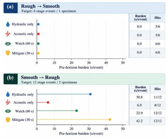
Across the 12 quantile/persistence combinations per horizon, rough-to-smooth Watch intercepted 6/6 throughout, Mitigate 2/6–6/6, and Hold 0/6–5/6. Reverse interception remained 12/12 for Watch and Mitigate and 10/12 for Hold, while early activity ranged from 6.3–27.0, 34.2–49.8, and 23.3–41.8 s/event. At q99, rough-to-smooth Hold detected 2/6, 1/6, 0/6, and 0/6 events at persistence of 1, 2, 3, and 5 s. The nominal 2 s result is therefore a sensitive diagnostic setting rather than a validated stopping rule (Supplementary Table S4). Figure 5 visualizes the corresponding relationship between pre-horizon alert exposure and event interception under the original source settings.

Figure 5. Event-window pre-horizon burden and interception under the original source settings: (a) rough-to-smooth transfer, with six target stage events from one specimen; (b) smooth-to-rough transfer, with twelve target stage events from two specimens. Both panels use the same burden axis; the right-hand columns give burden in s/event and intercepted-event counts. Burden measures indicator activity before the nominal horizon within selected 180 s windows, not false-alarm burden over months of quiet operation, performed interventions, or CO₂ throughput losses. The policies are ungated. Hold results are reported in Table 5.

4.3. Domain Support Changes the Interpretation of Predictive Success

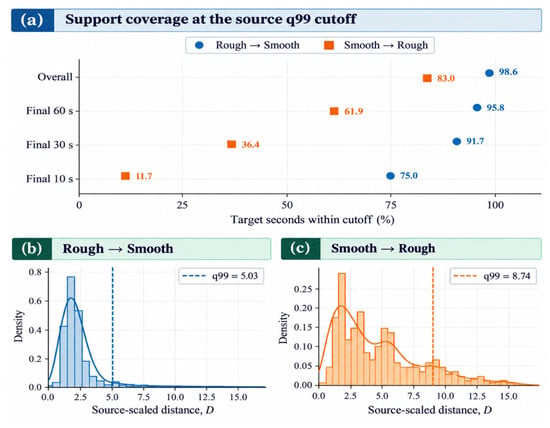
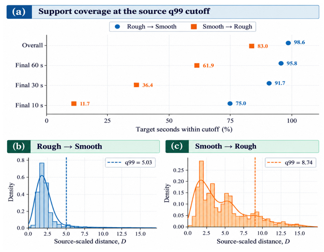
At the illustrative q99 Mahalanobis cutoff, overall support coverage was 98.6% for rough-to-smooth and 83.0% for smooth-to-rough transfer. Final 30 s coverage was 91.7% and 36.4%; final 10 s coverage was 75.0% and 11.7%. Conditional event-bootstrap intervals for the 30 s values are 90.6–92.8% and 19.4–54.7%, and for the 10 s values 71.7–78.3% and 0.0–31.7%. Even narrow intervals here reflect resampling of stages within the same specimens, not evidence of precise generalization to a new fault.

Median target distances were 2.30 and 4.38, with direction-specific source cutoffs of 5.03 and 8.74. These distances are calculated using different source scalings and covariance models and should not be interpreted on a common physical scale. The results show poor agreement between many near-peak rough states and the Mahalanobis envelope fitted to the smooth source. They do not establish that supported states are safe or that a lack of support implies an incorrect prediction. Table 6 summarizes the descriptive q99 support coverage and source/target distance statistics for both transfer directions. Figure 6 visualizes these coverage values together with the direction-specific target-distance distributions.

Table 6. Descriptive domain support at the illustrative q99 source cutoff. Values depend on the fitted source geometry; support is not safety certification.

Direction	Dcrit (q99)	Support-Eligible Overall (%)	≤60 s (%)	≤30 s (%)	≤10 s (%)	Median D Source (OOF)	Median D Target
Rough → Smooth	5.03	98.6	95.8	91.7	75.0	2.21	2.30
Smooth → Rough	8.74	83.0	61.9	36.4	11.7	1.79	4.38

Figure 6. Domain support at the illustrative source q99 cutoff. (a) Target coverage overall and in the final 60, 30, and 10 s windows. (b,c) Target-distance distributions for rough-to-smooth and smooth-to-rough transfer, respectively, with their own source-derived cutoffs. Distances are shown separately because the source scalings and covariance models differ; they are not a common physical scale. Coverage describes empirical similarity, not safety or prediction correctness. Results remain conditional on the original three specimens.

4.4. Support Gate Sensitivity

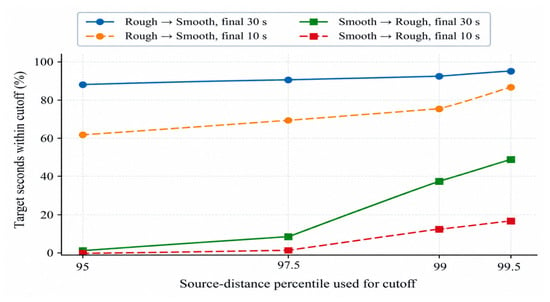
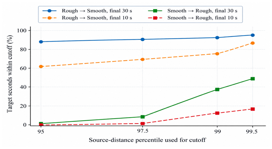
Coverage depends strongly on the chosen cutoff, particularly in smooth-to-rough transfer. Across q95–q99.5, coverage in the final 30 s increases from 87.2% to 95.0% for rough-to-smooth transfer and from 0.8% to 48.3% in reverse. The corresponding ranges for the final 10 s are 61.7–85.0% and 0.0–16.7%. The ordering is unchanged across this percentile family, but absolute support and the proposed review workload are not stable. This analysis describes the sensitivity of one distance formulation; it does not establish robustness to a different gate, source composition, or future specimen. Figure 7 shows how final-30-s and final-10-s support coverage changes across the evaluated source-distance percentile cutoffs.

Figure 7. Sensitivity of final-30-s and final-10-s target support to the empirical source-distance percentile. Symbols distinguish transfer directions and line styles distinguish the two windows. The same frozen target observations are evaluated at each cutoff. Absolute coverage changes substantially, especially in smooth-to-rough transfer; q99 is an illustrative reference, not an optimized or validated field operating threshold.

The additional robustness checks reproduce the original distances numerically but reveal instability in their calibration. Deleting one rough-source event and completely recalibrating yields smooth-target support of 90.6–93.9% in the final 30 s. Deleting one smooth-source event yields rough-target support of 19.7–88.6%. For rough-to-smooth/smooth-to-rough transfer, the diagonal robust gate gives 100.0%/63.1% coverage and the one-class SVM gives 97.2%/31.9%, compared with 91.7%/36.4% for Mahalanobis. Thinning source observations to 30 s intervals gives 85.6%/0.0%. Whole-rough-specimen calibration raises q99 from 5.03 to 9.47 and includes all smooth target states. Including more states within a different envelope does not establish better safety or prediction. Supplementary Tables S5–S8 and Figures S1–S3 report these sensitivities and score contributions.

4.5. Proposed Advisory Action Logic

Table 7 describes a proposed advisory mapping. The risk tier communicates the timing of an alarm, while the support flag communicates empirical similarity to source conditions. In this proposed mapping, all actions require operator assessment and an independently approved operating envelope; no actions were implemented in the experiments. Unsupported observations generate a review flag. The flag does not override physical alarms or establish that reduced automation is itself safe. Consequently, no fail-safe performance, authorized control class, or human-factors benefit is claimed.

Table 7. Proposed advisory decision matrix for the risk tier and empirical support flag. The action labels are conceptual and were not tested with operators or actuators.

Risk Tier	Horizon (s)	Supported Within Source-Distance Cutoff	Unsupported Beyond Source-Distance Cutoff
Normal	—	Review routine monitoring and physical constraints.	Check measurements and domain shift; a low score is not reassurance.
Watch	60	Review increased risk; consider closer monitoring.	Review the warning and verify input data promptly.
Mitigate	30	Review possible mitigation within approved operating limits.	Prioritize operator and physics assessment of the warning.
Hold	10	Urgent operator assessment; consider hold under approved rules.	Urgent operator and physics review; do not rely on the ML score alone.

Note: All tiers require operator judgment; no control action was tested. The dash denotes no forecast horizon for Normal. The support flag qualifies model evidence; it is not a safety assessment. Both supported and unsupported states remain subject to independent physical limits. Unsupported status calls for review of the learned model and must never disable alarms, interlocks, or an independently required safety response.

Table 7. Proposed advisory decision matrix for the risk tier and empirical support flag. The action labels are conceptual and were not tested with operators or actuators.

Risk Tier	Horizon (s)	Supported Within Source-Distance Cutoff	Unsupported Beyond Source-Distance Cutoff
Normal	—	Review routine monitoring and physical constraints.	Check measurements and domain shift; a low score is not reassurance.
Watch	60	Review increased risk; consider closer monitoring.	Review the warning and verify input data promptly.
Mitigate	30	Review possible mitigation within approved operating limits.	Prioritize operator and physics assessment of the warning.
Hold	10	Urgent operator assessment; consider hold under approved rules.	Urgent operator and physics review; do not rely on the ML score alone.

Note: All tiers require operator judgment; no control action was tested. The dash denotes no forecast horizon for Normal. The support flag qualifies model evidence; it is not a safety assessment. Both supported and unsupported states remain subject to independent physical limits. Unsupported status calls for review of the learned model and must never disable alarms, interlocks, or an independently required safety response.

Table 8 distinguishes implemented analytical components, retrospective checks, and untested design proposals. Statistical support, documentation, and concept diagrams do not validate live operation. The Hold indicator is included to expose its limited performance, not to imply readiness for automatic shutdown.

Table 8. Evidence status of the requirements. “Implemented” refers to offline code and does not mean field-validated or operationally approved.

ID	Requirement	Verification Evidence	Status
DR1	Traceable compact state	Raw interpolation and all 3240 feature rows audited.	Offline verified; online timing unvalidated
DR2	Horizon indicators	Fixed rules and 72 sensitivity cases; Hold misses retained.	Implemented offline only
DR3	Source settings	Thresholds/corrections reproduced from source OOF scores.	Implemented; no field optimum
DR4	Empirical support	Deletion, thinning, alternative gates and rough-specimen checks.	Implemented; substantial instability
DR5	Operator/physics fallback	Proposed Table 7 mapping.	Conceptual; not experimentally tested
DR6	Reproducibility	Versioned inputs, scripts, exact settings, environments, checksums.	Supplied archive; public link pending
DR7	Local interface	Risk/support/action semantics only.	Conceptual; no API or network test

Table 8. Evidence status of the requirements. “Implemented” refers to offline code and does not mean field-validated or operationally approved.

ID	Requirement	Verification Evidence	Status
DR1	Traceable compact state	Raw interpolation and all 3240 feature rows audited.	Offline verified; online timing unvalidated
DR2	Horizon indicators	Fixed rules and 72 sensitivity cases; Hold misses retained.	Implemented offline only
DR3	Source settings	Thresholds/corrections reproduced from source OOF scores.	Implemented; no field optimum
DR4	Empirical support	Deletion, thinning, alternative gates and rough-specimen checks.	Implemented; substantial instability
DR5	Operator/physics fallback	Proposed Table 7 mapping.	Conceptual; not experimentally tested
DR6	Reproducibility	Versioned inputs, scripts, exact settings, environments, checksums.	Supplied archive; public link pending
DR7	Local interface	Risk/support/action semantics only.	Conceptual; no API or network test

Table 9 reports all four percentile cutoffs so that the q99 example can be interpreted in context. A decision-maker would need to determine acceptable missed alerts and review workload using independent validation; the present data do not establish an optimal cutoff.

Table 9. Sensitivity of support-eligible coverage to the source domain support cutoff.

Direction	Source Quantile (%)	Dcrit	Support-Eligible Overall (%)	≤60 s (%)	≤30 s (%)	≤10 s (%)
Rough → Smooth	95.0	3.88	97.9	93.6	87.2	61.7
Rough → Smooth	97.5	4.64	98.2	94.7	89.4	68.3
Rough → Smooth	99.0	5.03	98.6	95.8	91.7	75.0
Rough → Smooth	99.5	5.71	99.2	97.5	95.0	85.0
Smooth → Rough	95.0	3.37	36.3	10.4	0.8	0.0
Smooth → Rough	97.5	6.01	65.7	35.8	8.1	0.0
Smooth → Rough	99.0	8.74	83.0	61.9	36.4	11.7
Smooth → Rough	99.5	9.93	89.3	71.1	48.3	16.7

Table 9. Sensitivity of support-eligible coverage to the source domain support cutoff.

Direction	Source Quantile (%)	Dcrit	Support-Eligible Overall (%)	≤60 s (%)	≤30 s (%)	≤10 s (%)
Rough → Smooth	95.0	3.88	97.9	93.6	87.2	61.7
Rough → Smooth	97.5	4.64	98.2	94.7	89.4	68.3
Rough → Smooth	99.0	5.03	98.6	95.8	91.7	75.0
Rough → Smooth	99.5	5.71	99.2	97.5	95.0	85.0
Smooth → Rough	95.0	3.37	36.3	10.4	0.8	0.0
Smooth → Rough	97.5	6.01	65.7	35.8	8.1	0.0
Smooth → Rough	99.0	8.74	83.0	61.9	36.4	11.7
Smooth → Rough	99.5	9.93	89.3	71.1	48.3	16.7

Supplementary Table S3 lists every target event and its warning outcome. Table 10 retains conditional event-level uncertainty summaries, and Figure 8 makes missed Hold events visible. The event, rather than the second, is the resampling block, but the independent experimental unit is the specimen. The original transfer cohort contains one smooth and two rough specimens; Section 4.7 reports the separate additional specimen.

Figure 8. Within-horizon warning times for all selected original-cohort target events. Each annotated cell gives warning time in seconds; a cross denotes noninterception, not a zero warning time. The upper six rows are smooth-target events, and the lower twelve rows are grouped by rough specimen. The color scale is shared across tiers. Complete Watch and Mitigate interception in these windows does not establish reliability on independent specimens; the Hold misses remain negative evidence.

Figure 8. Within-horizon warning times for all selected original-cohort target events. Each annotated cell gives warning time in seconds; a cross denotes noninterception, not a zero warning time. The upper six rows are smooth-target events, and the lower twelve rows are grouped by rough specimen. The color scale is shared across tiers. Complete Watch and Mitigate interception in these windows does not establish reliability on independent specimens; the Hold misses remain negative evidence.

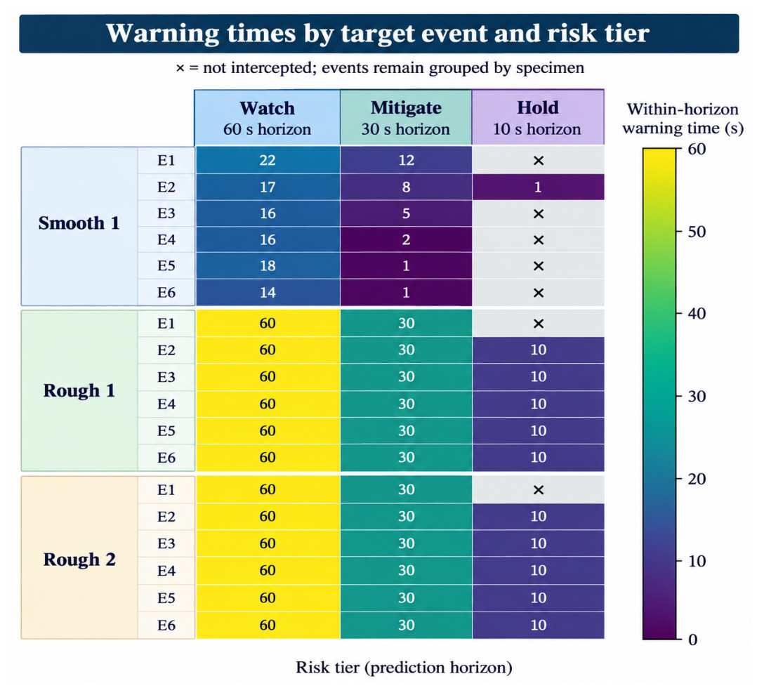
Table 10. Conditional event summaries. Wilson intervals are nominal binomial event-count reference intervals; event-bootstrap ranges retain within-event dependence only. Neither accounts for shared specimen history or establishes population coverage.

Direction	Metric	Estimate	Nominal 95% Range	Method	Event Unit	Interpretation
Rough to smooth	Watch event interception	100.0%	61.0 to 100.0%	Wilson reference	6 smooth events	Early tier interception
Rough to smooth	Watch median warning	16.5 s	15.0 to 20.0 s	Conditional event-bootstrap	6 smooth events	Warning timing
Rough to smooth	Mitigate event interception	100.0%	61.0 to 100.0%	Wilson reference	6 smooth events	Action tier interception
Rough to smooth	Mitigate median warning	3.5 s	1.0 to 10.0 s	Conditional event-bootstrap	6 smooth events	Action timing
Rough to smooth	Hold event interception	16.7%	3.0 to 56.4%	Wilson reference	6 smooth events	Observed Hold outcome
Smooth to rough	Watch pre-horizon burden	22.9 s/event	17.2 to 29.4 s/event	Conditional event-bootstrap	12 rough events	Early alert exposure
Smooth to rough	Mitigate pre-horizon burden	42.2 s/event	35.1 to 49.8 s/event	Conditional event-bootstrap	12 rough events	Early alert exposure
Rough to smooth	support-eligible coverage within 30 s	91.7%	90.6 to 92.8%	Conditional event-bootstrap	6 smooth events	Near event support
Rough to smooth	support-eligible coverage within 10 s	75.0%	71.7 to 78.3%	Conditional event-bootstrap	6 smooth events	Near-failure support
Smooth to rough	support-eligible coverage within 30 s	36.4%	19.4 to 54.7%	Conditional event-bootstrap	12 rough events	Near event support
Smooth to rough	support-eligible coverage within 10 s	11.7%	0.0 to 31.7%	Conditional event-bootstrap	12 rough events	Near-failure support

Table 11 presents separate summaries for each target group. It reports observed interception counts, interception percentages, and pre-horizon alert exposure for Watch, Mitigate, Hold, and the two reference policies. The groups differ in specimen replication; the summaries are descriptive and do not establish the superiority of either transfer direction. Table 5 provides AP values, warning times, and duty fractions for additional context.

Table 11. Event interception and pre-horizon alert exposure under the original source-calibrated policies. The two target groups are reported separately; the values describe selected 180 s event windows.

Policy	Horizon (s)	Events Intercepted (n/N)	Interception (%)	Pre-Horizon Burden (s/Event)
A. Rough-to-Smooth Transfer: Six Target Stage Events from One Smooth Specimen
Watch	60	6/6	100.0	0.0
Mitigate	30	6/6	100.0	0.0
Hold	10	1/6	16.7	0.0
Hydraulic-only	30	5/6	83.3	0.0
Acoustic-only	30	5/6	83.3	0.0
B. Smooth-to-rough transfer: twelve target stage events from two rough specimens
Watch	60	12/12	100.0	22.9
Mitigate	30	12/12	100.0	42.2
Hold	10	10/12	83.3	26.0
Hydraulic-only	30	11/12	91.7	30.8
Acoustic-only	30	8/12	66.7	6.0

Note: Interception counts, percentages, and pre-horizon burden are consistent with Table 5. Burden is the mean duration of indicator activity before the nominal horizon within each selected 180 s window. The policies are ungated; empirical support is evaluated separately. These summaries do not estimate months of quiet operation, field false-alarm rates, performed interventions, or measured CO₂ losses. Stages from the same specimen are repeated observations, not independent specimens.

4.6. Alert Activity in Archived Interstage Exposure

After the 30 s post-event exclusion, eligible exposure was 2097 s in the smooth target and 3806 s across the rough targets. Rough-to-smooth Watch was active for 6 s in one episode (0.29% duty); Mitigate and Hold were never active. Reverse Watch was active for 61 s in five episodes (1.60%), Mitigate for 34 s in three episodes (0.89%), and Hold for 0 s. All active seconds passed the original q99 support check. These short records show that zero event-window pre-horizon burden does not imply zero activity elsewhere. They do not establish a false-alarm rate over prolonged quiet field operation, and the support flag does not eliminate all interstage activity. Supplementary Table S9 gives the exposure definition, counts, and buffer sensitivity. Washout choice matters: at 0/30/60 s buffers, smooth-target Watch duty is 5.45%/0.29%/0.00% and Mitigate duty 3.07%/0.00%/0.00%; rough-target values are 2.09%/1.60%/1.25% and 1.99%/0.89%/0.67%. The 30 s buffer reflects feature memory, not a demonstrated physical reset.

With the annotation-independent fixed post-peak exclusion of 210 s, eligible exposure is 1430 s in the smooth record and 3028 s in the rough records. No smooth-target indicators are active; rough-target Watch and Mitigate are active for 33 and 16 s (1.09% and 0.53%), respectively, with no Hold activity. The same alert counts occur at 180 and 240 s exclusions as the available exposure changes. All active seconds pass the support gate, although 375 s of the rough-target exposure are unsupported. This sensitivity reduces dependence on the archived event-end labels and still does not establish long-term field false-alarm performance (Supplementary Table S11).

4.7. Independent Slow-Pressurization Transfer

For the six external SC2 peaks, the unchanged rough-source Watch indicator intercepted 5/6, with a median warning time of 45 s and 3.2 s/event of pre-horizon activity; Mitigate and Hold intercepted 0/6. Rough-source AP was 0.85, 0.76, and 0.34 for the three horizons. The unchanged smooth-source Watch, Mitigate, and Hold indicators intercepted 4/6, 6/6, and 3/6, with early activity of 39.2, 72.8, and 26.8 s/event and AP values of 0.68, 0.60, and 0.23, respectively. Warning times are calculated only for intercepted peaks; a tier that intercepts no peaks has no warning estimate. Supplementary Table S12 reports all settings.

The rough-source gate included 1077/1080 external states (99.7%) and 177/180 final-30-s states (98.3%); the smooth-source gate included every external state. Consequently, near-complete geometric support coexists with missed Mitigate peaks or extensive early activity, depending on the source policy. This independent example shows that similarity of measured state distributions does not establish transfer of the time-to-peak relationship or policy calibration. The comparison does not isolate pressurization rate from specimen and processing differences, and it does not validate field operating decisions.

5. Discussion

5.1. Risk Scores and Empirical Support Answer Different Questions

In smooth-to-rough transfer, the Watch and Mitigate indicators intercepted 12/12 events. However, q99 Mahalanobis coverage was 61.9% and 36.4% in the final 60 and 30 s, respectively, and 11.7% in the final 10 s. Thus, event ranking and inclusion within a particular source distribution can diverge on the same dataset. This result does not show that support gating improves safety or that the selected cutoff defines permissible control authority.

DT literature discusses real-time decisions and the need for reliable data integration [8,9,10]. The present offline results motivate carrying an empirical support diagnostic alongside a risk score in a future advisory application. Such a diagnostic can expose extrapolation relative to a chosen representation, but it remains sensitive to the representation, covariance model, source specimens, and threshold. Calibration and prospective outcome monitoring would still be required.

5.2. Source Composition and Limits of Cross-Fault Inference

The observed asymmetry is compatible with the two rough specimens sampling more varied trajectories than the single smooth specimen. However, roughness category, source specimen count, and specimen-specific history are confounded. The analysis cannot attribute the difference uniquely to roughness or demonstrate that adding a rough source generally improves transfer. Independent specimens spanning roughness, stress, injection rate, and sensor configurations are needed to separate these effects.

The smooth-source deletion results additionally show that the apparent magnitude of extrapolation depends on which pressure stages define the envelope. High lag-one correlation of the source distance (median 0.947 and 0.963 in rough and smooth events) confirms that thousands of rows do not supply thousands of independent calibration observations. Shrinkage, temporal thinning, and alternative gates explore this limitation without resolving the absence of independent specimens.

The external slow-pressurization evaluation strengthens this distinction. A high AP can coexist with no threshold interception, as for rough-source Mitigate (AP 0.76; 0/6), while complete interception can incur large early exposure, as for smooth-source Mitigate (6/6; 72.8 s/event). A support gate cannot certify conditional probability calibration or an appropriate intervention threshold. Any future field use therefore needs separate prospective calibration and policy validation even when measured states lie inside a source envelope.

Differences between distributions can contain physically relevant information, but an empirical distance alone does not identify the cause of those differences. A future application should retain provenance and descriptors of the fault, stress path, pressure rate, and sensors, then test their influence on independent cases. Domain adaptation or a more complex model would not remove the need for such validation.

5.3. Contribution to Intelligent Supply Chain Systems

CCUS network models address source–sink matching, capacity, and disruptions [1,2,3], while supply chain DT studies consider visibility, information exchange, and decision processes [6,7,8,9,10,11]. This study contributes only a proposed local information contract to that context. A risk indicator is not a direct estimate of available injection capacity and cannot by itself determine rerouting or contractual nominations.

A future site system could transmit the risk tier and support flag with timestamps, sensor quality, and operator review status. A network planning tool would require a separately validated mapping from the site assessment to admissible capacity before using it for flow allocation. That mapping, the API, and network integration are not implemented or tested here.

The study does not quantify network cost savings, avoided emissions, rerouting benefits, improvements in service availability, or effects on CO₂ throughput. Its scope remains the retrospective laboratory analysis and a conceptual local advisory interface.

5.4. Industry 5.0: Resilience, Sustainability, and Human-Centered Operation

Resilience, sustainability, and human-centered operation [12] are principles for future design, not demonstrated outcomes of this study. A resilience benefit would require evidence that acting on an alert reduces disruption. A sustainability benefit would require measured effects on carbon handling or energy use. Human-centered operation would require testing operator comprehension, workload, and decisions. Event-window burden and duty provide none of this evidence; their interpretation is therefore restricted to retrospective alert activity.

The compact variables, explicit thresholds, and simple logistic models make the analysis inspectable. Traceability is useful for reviewing how an alert arose, but transparency does not establish calibration, causal validity, or regulatory acceptability. Those properties require separate evidence.

5.5. Maturity of the Evaluated Prototype

The study uses real laboratory measurements [13,23], not simulated observations, but it provides no field validation. It is an offline prototype. A live digital shadow would require automatic physical-to-digital updates; a deployed twin would additionally require the relevant operational feedback and integration [4,5]. In the retained title, “Digital Twin Ready” refers to the intended design of a candidate analytical component for future digital-twin integration, not to demonstrated integration, field validation, or operational readiness. Neither a maturity level nor a technology readiness level is assigned.

Before deployment, the proposed workflow would need sensor synchronization and quality controls, prospective blind validation, a physical site model and approved limits, action logging, operator evaluation, and tests of control behavior. Physical constraints should remain independent of the learned risk indicator and distance gate. Table 12 is an untested development roadmap rather than a record of delivered capability.

Table 12. Proposed future validation and integration stages. Every row describes part of a development roadmap, not an implemented or empirically verified capability.

Stage	Required Capability	Deliverable
Laboratory confirmation	Replicated roughness/stress/rate matrix; prospective threshold freeze	Prospectively tested event definitions, state distributions, support gate
Pilot injection node	Live pressure/rate/deformation/seismic ingestion; physics hard limits	Future live digital shadow with advisory Watch/Mitigate/Hold
Governed closed loop	Preapproved rate/hold actions; operator confirmation; audit log	Future bidirectional twin with bounded automation
Supply chain integration	Expose node service state API to CCUS planning layer	Tested rerouting, nominations, and capacity management

5.6. Relationship to the Companion Geomechanics Study

The companion manuscript [24] and this study share the experimental archive and preprocessing. The companion addresses broad precursor prediction and cross-fault transfer; this work evaluates compact indicators, policy thresholds, alert exposure, and statistical support. Its contribution is limited to that secondary analysis and the proposed advisory interface. The unpublished companion manuscript is cited to disclose this overlap and is not used as independent validation.

5.7. Limitations and Next Steps

• The original 18 stage events are nested in three specimens. Six external stage peaks add one independent slow-pressurization specimen, yielding 24 evaluated trajectories across four specimens in total, reported as separate cohorts. The requested doubling to at least 36 events has not been achieved. Repeated stages, overlapping windows and resampling cannot increase specimen replication. Neither cohort supports precise population detection rates; the external record represents slow creep rather than six independent unstable earthquakes.
• Event-centered selection enriches the data for failure approach. The reported burden and duty do not estimate field false alarms, curtailment, or throughput loss. Any additional outside window exposure remains a short laboratory diagnostic and cannot substitute for months of prospective monitoring.
• The horizons, negative score quantiles, persistence times, and support percentiles are illustrative laboratory choices. Sensitivity analysis describes their effects on these records; target outcomes have not been used to select a new preferred operating point. Field timing would require evidence about physical timescales and response latency.

6. Conclusions

This secondary analysis constructs and evaluates seven physically interpretable laboratory risk variables, source-calibrated persistent indicators, and a separate statistical support diagnostic. The contribution is an offline method with explicitly documented limitations rather than a validated injection controller or deployed digital twin. In rough-to-smooth transfer, the Watch and Mitigate indicators intercepted 6/6 selected events, with median warning times of 16.5 and 3.5 s, respectively, and no pre-horizon alert activity within the selected event windows. However, the nominal Wilson event-count interval of 61.0–100.0% and the use of a single target specimen preclude a precise general detection claim. In smooth-to-rough transfer, Watch and Mitigate intercepted 12/12 selected events but produced 22.9 and 42.2 s/event of early alert activity, respectively, demonstrating that event interception must be considered together with the duration and timing of alerts; these quantities do not represent actual interventions or losses of field service. At the illustrative q99 Mahalanobis cutoff, final-30-s support coverage was 91.7% and 36.4% for rough-to-smooth and smooth-to-rough transfer, respectively. Support coverage depends on the selected cutoff, source composition, and distance model and should therefore be interpreted as an empirical diagnostic rather than a safety or operational permission rule. Consistent with this limitation, deletion sensitivity changed smooth-source final-30-s support coverage to 19.7–88.6%, demonstrating substantial dependence on the source events. The 10 s indicator also missed five of the six smooth-target events and is therefore not validated for automatic Hold actions. Additional independent specimens, prospective non-event exposure, and field and operator evaluations are required before operational use. The additional independent specimen provides six slow-creep stage peaks, increasing the total evaluation to 24 trajectories across four specimens, and reveals policy-transfer failures despite 99.7–100.0% overall domain-support coverage. These findings demonstrate that warning thresholds and calibration must be validated separately from domain similarity. Overall, the results support retaining separate risk and empirical-support information for further advisory testing while preserving independent physical constraints; however, the sample remains below the requested doubling, and the present evidence does not establish field or operational readiness.

References

- Zhang, S.; Liu, L.; Zhang, L.; Zhuang, Y.; Du, J. An optimization model for carbon capture utilization and storage supply chain: A case study in Northeastern China. Appl. Energy 2018, 231, 194–206. [Google Scholar] [CrossRef] [Scilit]
- d’Amore, F.; Sunny, N.; Iruretagoyena, D.; Bezzo, F.; Shah, N. European supply chains for carbon capture, transport and sequestration, with uncertainties in geological storage capacity: Insights from economic optimisation. Comput. Chem. Eng. 2019, 129, 106521. [Google Scholar] [CrossRef] [Scilit]
- Lei, W.; Zhang, W.; Zhu, J. Optimal Design of Resilient Carbon Capture, Utilization and Storage (CCUS) Supply Chain Networks under Facility Disruption. Sustainability 2024, 16, 2621. [Google Scholar] [CrossRef] [Scilit]
- Kritzinger, W.; Karner, M.; Traar, G.; Henjes, J.; Sihn, W. Digital Twin in manufacturing: A categorical literature review and classification. IFAC-PapersOnLine 2018, 51, 1016–1022. [Google Scholar] [CrossRef] [Scilit]
- Fuller, A.; Fan, Z.; Day, C.; Barlow, C. Digital Twin: Enabling Technologies, Challenges and Open Research. IEEE Access 2020, 8, 108952–108971. [Google Scholar] [CrossRef] [Scilit]
- Ivanov, D.; Dolgui, A. New disruption risk management perspectives in supply chains: Digital twins, the ripple effect, and resileanness. IFAC-PapersOnLine 2019, 52, 337–342. [Google Scholar] [CrossRef] [Scilit]
- Zaidi, S.A.H.; Khan, S.A.; Chaabane, A. Unlocking the potential of digital twins in supply chains: A systematic review. Supply Chain Anal. 2024, 7, 100075. [Google Scholar] [CrossRef] [Scilit]
- Roman, E.-A.; Stere, A.-S.; Roșca, E.; Radu, A.-V.; Codroiu, D.; Anamaria, I. State of the Art of Digital Twins in Improving Supply Chain Resilience. Logistics 2025, 9, 22. [Google Scholar] [CrossRef] [Scilit]
- Liu, C.; Wang, Y.; Purvis, L.; Potter, A. Can Digital Twin Technology Enhance Supply-Chain Resilience? A Systematic Literature Review. Sustainability 2026, 18, 2361. [Google Scholar] [CrossRef] [Scilit]
- Tolia, A.; Ponis, S.T. Digital Twins for Real-Time Decision-Making in Supply Chain Management and Logistics: A Systematic Review. Information 2026, 17, 732. [Google Scholar] [CrossRef] [Scilit]
- Li, S.; Jin, P.; Su, S.; Yao, J.; Pang, Q. Digital Twins and Cross-Border Logistics Systems Risk Management Capability: An Innovation Diffusion Perspective. Systems 2025, 13, 658. [Google Scholar] [CrossRef] [Scilit]
- Breque, M.; De Nul, L.; Petridis, A. Industry 5.0: Towards a Sustainable, Human-Centric and Resilient European Industry; Publications Office of the European Union: Luxembourg, 2021. [Google Scholar] [CrossRef] [PubMed]
- Wang, L.; Kwiatek, G.; Renard, F.; Guérin-Marthe, S.; Rybacki, E.; Bohnhoff, M.; Naumann, M.; Dresen, G. Fault roughness controls injection-induced seismicity. Proc. Natl. Acad. Sci. USA 2024, 121, e2310039121. [Google Scholar] [CrossRef] [Scilit] [PubMed]
- Zoback, M.D.; Gorelick, S.M. Earthquake triggering and large-scale geologic storage of carbon dioxide. Proc. Natl. Acad. Sci. USA 2012, 109, 10164–10168. [Google Scholar] [CrossRef] [Scilit] [PubMed]
- Guglielmi, Y.; Cappa, F.; Avouac, J.-P.; Henry, P.; Elsworth, D. Seismicity triggered by fluid injection-induced aseismic slip. Science 2015, 348, 1224–1226. [Google Scholar] [CrossRef] [Scilit] [PubMed]
- Cappa, F.; Scuderi, M.M.; Collettini, C.; Guglielmi, Y.; Avouac, J.-P. Stabilization of fault slip by fluid injection in the laboratory and in situ. Sci. Adv. 2019, 5, eaau4065. [Google Scholar] [CrossRef] [Scilit] [PubMed]
- Schultz, R.; Skoumal, R.J.; Brudzinski, M.R.; Eaton, D.; Baptie, B.; Ellsworth, W. Hydraulic fracturing-induced seismicity. Rev. Geophys. 2020, 58, e2019RG000695. [Google Scholar] [CrossRef] [Scilit]
- Kwiatek, G.; Saarno, T.; Ader, T.; Bluemle, F.; Bohnhoff, M.; Chendorain, M.; Dresen, G.; Heikkinen, P.; Kukkonen, I.; Leary, P.; et al. Controlling fluid-induced seismicity during a 6.1-km-deep geothermal stimulation in Finland. Sci. Adv. 2019, 5, eaav7224. [Google Scholar] [CrossRef] [Scilit] [PubMed]
- Hill, R.G.; Weingarten, M.; Langenbruch, C.; Fialko, Y. Mitigation and optimization of induced seismicity using physics-based forecasting. J. Geophys. Res. Solid Earth 2024, 129, e2024JB028759. [Google Scholar] [CrossRef] [Scilit]
- Rouet-Leduc, B.; Hulbert, C.; Lubbers, N.; Barros, K.; Humphreys, C.J.; Johnson, P.A. Machine learning predicts laboratory earthquakes. Geophys. Res. Lett. 2017, 44, 9276–9282. [Google Scholar] [CrossRef] [Scilit]
- Vo Thanh, H.; Dai, Z.; Zhang, T. Toward Real-Time Digital Twins for CO2 Storage: Graph Neural Network Ensembles for Multi-physics Forecasting and Risk Quantification. In Rock Mechanics and Rock Engineering; Springer: Berlin/Heidelberg, Germany, 2026. [Google Scholar] [CrossRef] [Scilit]
- Shoeibi Omrani, P.; Octaviano, R.; Poort, J.; Palochis, D.; Hashemi, L.; Egberts, P.; Dashtaki Hesari, H. Digital Twin of Geothermal Assets Assisting the Production and Operational Decisions. GeoTHERM J. 2024, 2. Available online: https://www.geotherm-journal.com/index.php/gtjw/article/view/216 (accessed on 29 September 2026).
- Wang, L. Supplementary Data for the study of ‘Injection-induced seismicity controlled by fault roughness’. Mendeley Data, Version 1. 2023. Available online: https://data.mendeley.com/datasets/xcyvspjk3c/1 (accessed on 14 October 2026).
- Akpabli, G.; Rahnema, H.; Marfo, W.A.; Hayford, K. Mechanics-Informed Machine Learning Identifies Asymmetric Cross-Fault Generalization of Fluid-Induced Slip Precursors.
- Wang, L.; Kwiatek, G.; Rybacki, E.; Bonnelye, A.; Bohnhoff, M.; Dresen, G. Laboratory Study on Fluid-Induced Fault Slip Behavior: The Role of Fluid Pressurization Rate. Geophys. Res. Lett. 2020, 47, e2019GL086627. [Google Scholar] [CrossRef] [Scilit]
- Wang, L.; Kwiatek, G.; Rybacki, E.; Bonnelye, A.; Bohnhoff, M.; Dresen, G. Data of fluid-induced fault slip experiments. Figshare, Version 3. 2020. Available online: https://figshare.com/articles/dataset/testSC1_xlsx/11948739/3 (accessed on 14 October 2026).
- Hevner, A.R.; March, S.T.; Park, J.; Ram, S. Design Science in Information Systems Research. MIS Q. 2004, 28, 75–105. [Google Scholar] [CrossRef] [Scilit]
- Peffers, K.; Tuunanen, T.; Rothenberger, M.A.; Chatterjee, S. A Design Science Research Methodology for Information Systems Research. J. Manag. Inf. Syst. 2007, 24, 45–77. [Google Scholar] [CrossRef] [Scilit]
- James, G.; Witten, D.; Hastie, T.; Tibshirani, R.; Taylor, J. An Introduction to Statistical Learning: With Applications in Python; Springer: Cham, Switzerland, 2023. [Google Scholar] [CrossRef] [Scilit]
- Van Calster, B.; Nieboer, D.; Vergouwe, Y.; De Cock, B.; Pencina, M.J.; Steyerberg, E.W. A calibration hierarchy for risk models was defined: From utopia to empirical data. J. Clin. Epidemiol. 2016, 74, 167–176. [Google Scholar] [CrossRef] [Scilit] [PubMed]
- Roberts, D.R.; Bahn, V.; Ciuti, S.; Boyce, M.S.; Elith, J.; Guillera-Arroita, G.; Hauenstein, S.; Lahoz-Monfort, J.J.; Schröder, B.; Thuiller, W.; et al. Cross-validation strategies for data with temporal, spatial, hierarchical, or phylogenetic structure. Ecography 2017, 40, 913–929. [Google Scholar] [CrossRef] [Scilit]
- Ledoit, O.; Wolf, M. A well-conditioned estimator for large-dimensional covariance matrices. J. Multivar. Anal. 2004, 88, 365–411. [Google Scholar] [CrossRef] [Scilit]
- Cabana, E.; Lillo, R.E.; Laniado, H. Multivariate outlier detection based on a robust Mahalanobis distance with shrinkage estimators. Stat. Pap. 2021, 62, 1583–1609. [Google Scholar] [CrossRef] [Scilit]
- Schölkopf, B.; Platt, J.C.; Shawe-Taylor, J.; Smola, A.J.; Williamson, R.C. Estimating the Support of a High-Dimensional Distribution. Neural Comput. 2001, 13, 1443–1471. [Google Scholar] [CrossRef] [Scilit] [PubMed]
- Saito, T.; Rehmsmeier, M. The precision-recall plot is more informative than the ROC plot when evaluating binary classifiers on imbalanced datasets. PLoS ONE 2015, 10, e0118432. [Google Scholar] [CrossRef] [Scilit] [PubMed]
- Dimitriadis, T.; Gneiting, T.; Jordan, A.I. Stable reliability diagrams for probabilistic classifiers. Proc. Natl. Acad. Sci. USA 2021, 118, e2016191118. [Google Scholar] [CrossRef] [Scilit] [PubMed]
- Guo, C.; Pleiss, G.; Sun, Y.; Weinberger, K.Q. On Calibration of Modern Neural Networks. In Proceedings of the 34th International Conference on Machine Learning, Sydney, Australia, 6–11 August 2017; PMLR: Cambridge, MA, USA; Volume 70, pp. 1321–1330. Available online: https://proceedings.mlr.press/v70/guo17a.html (accessed on 14 October 2026).
- McGrath, O.; Burke, K. Binomial Confidence Intervals for Rare Events: Importance of Defining Margin of Error Relative to Magnitude of Proportion. Am. Stat. 2024, 78, 437–449. [Google Scholar] [CrossRef] [Scilit]
Disclaimer/Publisher’s Note: The statements, opinions and data contained in all publications are solely those of the individual author(s) and contributor(s) and not of MDPI and/or the editor(s). MDPI and/or the editor(s) disclaim responsibility for any injury to people or property resulting from any ideas, methods, instructions or products referred to in the content. |
© 2026 by the authors. Licensee MDPI, Basel, Switzerland. This article is an open access article distributed under the terms and conditions of the Creative Commons Attribution (CC BY) license.