


Highlights
Please indicate how your work links to systems science via your contributions to systems practice, theory, and/or methodology.
- Explicit control paths distinguish planning access, inertia, task filling, and shared safety intervention.
What are the main findings and/or the implications of the main findings?
- In the evaluated simulations under fixed inertia, event-gated planning with closed-gate filling improves completion and reduces ordinary planning access and plan changes relative to always-open planning but increases flight energy per completed order.
- The completion advantage reverses without closed-gate filling, indicating an architecture-dependent trade-off; service, energy, and plan changes should be evaluated jointly.
Abstract
Dynamic drone delivery requires rules for retaining and revising released plans. We specify a closed-loop architecture separating ordinary replanning access, assignment-change penalties, and shared safety intervention, while explicitly identifying closed-gate task filling. Three role-differentiated drones and a mobile support platform are evaluated using demand and weather proxies on all 88 eligible holdout dates. Four policies cross always-open or event-gated access with fixed or adaptive inertia. A paired NoFill intervention removes ordinary closed-gate filling without disabling planned execution or safety checks. Full factorial effects and calendar-block uncertainty replace the original selected-contrast, independent-date analysis. With fixed inertia, the Original event-gated policy increases completion by 5.806 percentage points (seven-day block 95% interval: 4.016 to 7.601) but increases flight energy by 10.414 Wh per completed order. Without filling, its completion difference is −3.431 points (−5.187 to −2.005). Ordinary planning access and assignment changes remain lower. Incremental adaptive-inertia benefits under event-gated access are unresolved. The results identify a conditional architectural trade-off, not a pure replanning-frequency benefit. The fixed simulation window, transferred physical inputs, and unmodelled operational constraints limit inference beyond this setting.
1. Introduction
1.1. Operational Problem and System Under Study
Dynamic UAV delivery requires rules for released plans as well as routes [1,2,3]. A released commitment is a published, unexecuted order–UAV–slot assignment. Ordinary planning access authorises global replanning, while inertia penalises assignment changes when planning opens. A shared safety mechanism checks first-slot executability before ordinary gating and before execution. Demand and deadlines motivate revision; wind, energy, and platform position constrain it. The governance question concerns service responsiveness, plan changes, and resource use.
One mobile platform supports launch, recovery, and battery swapping for three role-differentiated UAVs. Following the system/actor distinction [4], dispatcher rules govern planning and execution. Each sortie returns to the step-start platform before inter-step relocation. A shared MILP assigns arrived orders when planning opens. The platform does not serve customers or participate in road-route optimisation; its realised trajectory can differ across policies under the common relocation rule.
1.2. Research Gap, Evidence Boundary, and Safety Mechanism
Truck–UAV studies address routing, synchronisation, and allocation [5,6,7,8,9,10,11,12,13,14,15,16]; dynamic-routing frameworks distinguish information revelation from decision timing [17,18]. Event-triggered control motivates state-dependent updating [19]. We distinguish planning access from penalties applied after access, and from execution admissibility. Section 2 and Supplementary Table S2 delimit the contribution.
The evaluation separates input proxies from assumptions. São Paulo order and weather sources constrain arrival timing and wind; destinations and VIP labels are constructed. Separately sourced M100 data supply an external power reference, not fleet telemetry. W3 is a design weight, not measured coordination cost; Section 3 defines the plan-change accounting.
Safety intervention is separate from discretionary replanning [20]. Updated wind, energy, or eligibility can invalidate a first-slot task. ForcedSafetyTrigger then initiates replanning or deterministic fallback (Section 3.4). Rejected execution attempts are counted as risk aborts, not unsafe flights performed.
1.3. Inferential Design, Research Questions, and Contributions
We specify how state evidence enters ordinary planning access, assignment-change preferences, closed-gate filling, and safety intervention. These are distinct control paths, but the Original ET policy couples gated access with an additional filling path. The revision tests that coupling rather than treating the Original access contrast as a pure frequency intervention. Two research questions guide the analysis.
RQ1: Under shared physical and safety rules, how do the four access-by-inertia policies differ in VIP on-time performance, completion, flight energy per completed order, ordinary planning access, and policy-labelled assignment changes, and how do these differences change when ordinary closed-gate filling is removed?
RQ2: What conditional policy-choice implications follow from these joint outcomes when no universal management utility function or field-validity claim is assumed?
AlwaysFixed, ETFixed, AlwaysAdaptive, and ETAdaptive form the 2 × 2 design; AlwaysMyopic is a nonfactorial zero-inertia reference. For both Original and NoFill, we report all four simple contrasts, both main effects, and the access-by-inertia interaction. NoFill removes the ordinary filling procedure only. All comparisons hold exogenous inputs, model parameters, solver settings, and the shared safety mechanism constant within a date.
The revised evaluation uses every one of the 88 eligible holdout dates under the development-set P90 wind-residual gate. The original 60 dates are a deterministic subset, not a random or independently validating sample. Policy differences are paired within date and averaged with equal date weights. Calendar-block resampling retains gaps and addresses temporal dependence under explicit process assumptions; Section 4.1 and Section 4.2 define the estimator, main and interaction effects, and three-, seven-, and fourteen-day block analyses.
The systems contribution is evidence that the observed service benefit of restricting routine optimisation depends on the allocation path retained outside it. In this simulation, removing ordinary closed-gate filling reverses the fixed-inertia completion contrast, while ordinary planning access and plan changes remain lower. Complete factorial reporting distinguishes average policy effects from interactions; plan-change ledgers separate accounting categories, not causal mechanisms. The resulting service–energy–intervention profile supports conditional architecture evaluation rather than an algorithmic winner.
Original ETFixed improves completion relative to AlwaysFixed while reducing ordinary access and plan changes, but it consumes more energy per completed order. Removing ordinary closed-gate filling reverses the completion difference. The Original benefit therefore belongs to the bundled architecture rather than reduced replanning alone. Incremental Adaptive effects under ET remain unresolved across the five focal outcomes. Section 5 and Section 6 report the effects, uncertainty, and operational boundaries.
2. Literature Review and Research Positioning
2.1. Truck-UAV Coordination, Dynamic Delivery, and Mobile Platforms
Truck–UAV formulations integrate routing, allocation, and synchronisation. Flying Sidekick routing coordinates truck travel and UAV delivery [21]; two-echelon models permit repeated drone trips [22]; multi-visit pickup-and-delivery includes precedence, payload, and endurance [23]. These decision spaces differ from released-plan governance.
Multi-agent reinforcement learning also represents coordinated truck–UAV decisions [24]. Here, rules surrounding a common planner vary ordinary access and assignment-change penalties. Published performances are not directly comparable across these settings. Supplementary Table S2 records alignment requirements for a future external benchmark.
Dayarian et al. [25] model drones resupplying customer-serving trucks during stops. Here, UAVs serve customers and the platform supports sorties; platform customer service and road routing are excluded.
2.2. Rolling Planning, Event Triggers, and Exception Management
Dynamic routing separates evolving information from decisions [17,18]. Event-triggered platooning adjusts communication to state and bandwidth [19], while emergency truck–drone logistics uses an event-driven Markov game [26]. We examine update timing through an event-and-plan-age gate, not these domains’ control or routing algorithms.
The system/actor distinction [4] motivates explicit dispatcher functions: ordinary access, change preferences, and feasibility checks. Safety overrides and closed-gate filling are separate exceptions to routine optimisation.
2.3. Plan Stability, Exception Handling, and the Shared Safety Guard
Rescheduling studies measure completion-time deviations [27], changes across railway possession plans [28], and production-planning nervousness [29]. We likewise report service and plan changes separately. Hs is assignment distance, partitioned into policy- and safety-labelled ledgers; W3 is an objective weight (Section 3.2).
Wind- and energy-sensitive planning requires explicit feasibility checks [30,31,32,33]. Systems safety [20], UAV monitoring [34], and runtime assurance [35] motivate a distinct protective path. Our first-slot checks trigger replanning or fallback; they do not inherit formal assurance guarantees.
2.4. Research Positioning and Testable Comparisons
The experiment crosses ordinary access (Always or ET) with inertia (Fixed or Adaptive). Original ET additionally has a closed-gate filling path; NoFill makes the access comparison without that path. Full main effects and the interaction are reported for both versions, with all simple effects retained. Common exogenous inputs do not imply identical realised battery states, platform locations, or backlogs, so the contrasts represent complete closed-loop policies rather than static objective terms. Section 3.3 and Section 3.4 define the comparison.
Five focal outcomes retain different meanings: VIP on-time rate, completion, energy per completed order, policy-labelled plan changes, and ordinary access. AlwaysMyopic is a zero-inertia, nonfactorial reference. No universal utility or policy ranking is assumed.
3. System Definition, Decision Model, and Policy Architecture
This section specifies operating boundaries, observable state, planning, and safety paths. Supplementary Nomenclature, Table S1 and Algorithm S1 provide full symbols, settings, and execution details.
3.1. System Boundary, Actors, and Rolling Decision Sequence
One mobile support platform serves three model-defined UAV roles: capacity support, priority service, and contingency reserve. Roles specify allocation eligibility, not geographical territories, airframe types, or different payload ratings. The three roles share a compatible-order payload assumption but have distinct assumed energy multipliers (Section 3.2). These coefficients are not measured evidence of homogeneous aircraft performance. Archived two- and four-UAV configurations remain diagnostics, not fleet-size optimisation.
All UAVs and the platform are assumed technically available at every decision step. Equipment failure probabilities, repair crews, self-repair, maintenance downtime, emergency return after mechanical failure, and fault-related loss or recovery of payload are not simulated. A mission rejected by a flight or energy check is not a simulated mechanical breakdown; its order remains pending while lifecycle-eligible. Accordingly, this model cannot determine the route or payload outcome following an equipment fault.
Orders are allocated centrally from a shared backlog across the abstract service area. UAVs are not assigned exclusive territories and do not independently compete for orders. Slot capacity and order-uniqueness constraints prevent duplicate assignment; role eligibility and forecast feasibility determine which UAV can serve a candidate. Geographic zones describe demand locations, not ownership or service partitions.
Only outbound delivery is represented: a UAV takes an order from the platform to its destination and returns to the same platform location. There are no customer pickup requests, returns, or backhaul loading decisions. The return leg is therefore not reverse logistics. An extension would need pickup–delivery precedence, changing onboard payload, platform inventory, and compatible time and energy checks; these mechanisms are outside the current evaluation.
At each decision epoch, available information includes the platform location, UAV energies, arrived-order records, forecast wind, current observed wind, the shifted plan, and plan age. Candidate flight feasibility uses forecast wind. Current observed wind supplies the residual for ordinary gating and adaptive W3 and supports first-slot validation; it can therefore affect planning through access and the objective weight. Future arrivals and future realised wind are excluded from policy decisions. Only the final validated first slot is eligible for execution; the remaining two slots are provisional published assignments.
Each step incorporates arrivals, updates order status, and checks the shifted first-slot assignments. An ordinary trigger or a failed pre-check opens the shared planner. Otherwise the Original version retains existing assignments and may fill empty slots; NoFill retains the assignments without these additions. Both versions then validate the first slot under current replay wind and invoke the same deterministic safety fallback if required. Accepted sorties depart from and return to the step-start platform location. The platform relocates after execution and the remaining plan shifts forward. Figure 1 shows the Original control paths.
Figure 1.
Physical boundary and Original control paths. (a) Illustrative sorties depart from Pk and return before relocation to Pk+1; the paths need not operate simultaneously. Gray circles denote standard customers, and the red star denotes a priority customer. (b) State updates precede first-slot checking and the ordinary gate gk. An active gate or failed pre-check opens planning; otherwise, the shifted plan is retained with idle-slot filling. NoFill disables only this ordinary closed-gate filling branch. Both versions retain the final check, deterministic safety fallback, execution, and state feedback. Road routing and moving-platform recovery are excluded.
After execution, the platform moves at most 3.8 km toward the centroid of pre-execution first-slot destinations, or eligible backlog if none exists; with neither, it stays. The rule is common, but trajectories are endogenous. Road travel time, platform energy, congestion, in-motion charging, and spare-battery inventory are absent; the cap does not establish timing feasibility.
3.2. State, Order Lifecycle, Flight Feasibility, and Performance Metrics
The model distinguishes the information available for decisions, the tasks eligible for service, and the outcomes recorded after execution. All policies use the same information structure and exogenous replay, although their realised states can diverge. At decision step k, the observable state is defined by Equation (1).
Here, rk is platform location; Ek is the UAV-energy vector in Wh; Ok contains arrived-order records; wfk is the three-slot wind forecast; and wak is current replay wind. Π−k denotes the previous plan shifted forward by one slot, and Aplank is its age. Candidate feasibility uses forecast wind. Current wind affects the access gate, adaptive W3, and first-slot validation; it is not used as future realised wind.
Only arrived orders enter planning; future slots use forecasts, not future realised wind. During 12 clearance steps after arrivals, both wind series retain their final arrival-step values, an assumption rather than extra observations.
Standard and VIP orders have deadlines six and two steps after arrival, respectively. Deadlines are soft: an unserved order remains eligible through deadline +12 and expires at the next step, while remaining in arrival-based denominators. Each UAV-slot holds at most one order, and each order appears once at most.
Role eligibility adds a separate restriction. Forecast-based planning and idle-slot filling restrict the reserve UAV to VIP orders, orders waiting at least two steps, or slots with forecast wind ≥ 11 m/s. The deterministic safety fallback relaxes this role restriction but retains lifecycle and physical checks.
Planning and execution share a reduced-form round-trip flight model, using slot-specific forecast wind and current replay wind, respectively. Let e be the outbound unit direction and c the wind vector in m/s. Define c∥ = c·e and c⊥ = ‖c − c∥e‖. Airspeed is va = 62/3.6 m/s. The same steady wind applies to both legs, giving the track-holding ground speeds in Equation (2).
The track-holding component offsets crosswind, while along-track wind assists one leg and opposes the other. For positive-distance missions, feasibility requires c⊥ < va and both ground speeds ≥ 2.5 m/s. Wind direction and speed therefore affect mission duration, energy, planning access, and execution admissibility. The model uses planar distances and a steady wind vector for each evaluated sortie. Elevation, climbing and descending, terrain clearance, obstacles, altitude-dependent wind, gusts, rain, temperature, and icing are not represented. Consequently, the replay assesses the implemented wind-sensitive decision rules, not all-weather or hilly terrain flight capability.
Tqdk = 1000ℓqk(1/vout + 1/vret); ΔEqdk = 407.723375ηd Tqdk/3600
In Equation (3), ℓqk is one-way distance in km, Tqdk is round-trip duration in seconds, and ΔEqdk is energy in Wh. The main reference power is P_ref = 407.723375 W, the median record-level mean power in the 161-record M100 training set. This equivalent-power approximation does not represent activity-specific battery behaviour [36]. A zero-distance task is assigned zero duration and energy.
The M100 data [37] provide the external energy reference. The training set contains 148 route-flight records, nine ancillary ground tests, and four hovering tests; 48 route-flight records are held out by date. Reference-power percentiles are therefore derived from mixed operating states rather than a pure-cruise sample. Table S1 specifies the split.
Assumed role multipliers ηd = 1.05, 0.90, and 1.40 scale the common external power reference; they are not calibrated role-specific or same-airframe measurements. Feasible tasks require duration ≤ 1200 s and post-task energy ≥ 200 Wh. An assigned UAV with energy ≤ 480 Wh swaps to 1000 Wh before flight.
The maximum time-feasible mission energy is 190.27 Wh, so the 200 Wh reserve is non-binding under conditional swapping. One order per UAV-slot is an assignment limit, not a kilogram capacity. Orders are assumed compatible with a common payload envelope; order weights, numerical UAV maximum payload, platform aggregate payload, and inventory limits are not represented. The capacity-support role does not mean greater lifting capacity. Payload-dependent power, takeoff/landing energy, swap duration, and platform energy are absent. The model compares plan-governance rules conditional on compatible orders; it cannot determine physical maximum payload or establish robustness to mass and inventory constraints.
Equation (4) defines the service and energy outcomes evaluated jointly with Hs,policy and ordinary planning-access rate.
VIPOT = 100NVIP,on−time/NVIP; CR = 100Ncompleted/Narrived; EPO = Eflight/Ncompleted
VIPOT and CR are percentages of all arrived VIP and all arrived orders, including unserved/expired orders. EPO is executed-flight energy per completed order (Wh/order). Service, plan-change, and access use 88 dates. EPO uses the common 87-date subset with completions in all nine runs, excluding 30 August 2018; undefined ratios are not set to zero. Supplementary Table S9 additionally reports completed-order counts, total flight energy, and total/policy/safety plan changes on all 88 dates. EPO is conditional on service and this eligibility rule, not a standalone efficiency ranking.
Let D(Πk, Π−k) count changes between the final accepted plan and its shifted predecessor. An insertion into an empty slot or a deletion contributes one; replacement contributes two. Initial plan creation is included. Thus, the distance measures assignment changes, not exclusively disruption of existing commitments.
Hs = Hs,policy + Hs,safety
Equation (5) sums these endpoint distances over 39 steps; intermediate candidate plans are not counted. The multiplier 10 is shared with the MILP penalty 10W3∑z. Because this penalty also covers new assignments, W3 is not a pure retention-only intervention. Hs remains a structural index rather than observed workload or monetary cost.
Equation (6) is an accounting partition. If either the pre-gating or final first-slot check triggers safety intervention, the entire step’s distance enters Hs,safety; otherwise, it enters Hs,policy. Safety-labelled steps may therefore include changes generated by ordinary planning. The components are mutually exclusive by convention, not estimates of separate causal contributions.
All access and intervention rates use 39 decision steps as denominator. Ordinary planning access counts steps with an ordinary trigger and no pre-gating safety trigger, even if no candidate exists. Forced-safety rate counts steps with either safety trigger. A final safety trigger can therefore overlap ordinary planning access.
Sorties, swaps, and minimum battery energy are recorded separately. The execution function rejects tasks failing its flight, duration, or energy checks without flight-energy consumption or order completion. RiskAbortRate and UnsafeExecutionRate both report these rejection events per 100 arrived orders—not unsafe flights per attempted sortie. Their values are zero in all main Guard-ON runs; this does not establish field safety.
3.3. Policy Architectures and the Shared MILP
The four factorial policies cross ordinary planning access with the assignment-change penalty: AlwaysFixed (AF), ETFixed (EF), AlwaysAdaptive (AA), and ETAdaptive (EA). Always permits replanning at each step; ET uses the event-and-plan-age gate. Fixed holds W3 constant, whereas Adaptive updates it from the observed state when the planner opens. All share the MILP, flight model, role restrictions, and safety checks. In Original, ET also has the closed-gate filling procedure described in Section 3.4. Thus, the Original access factor changes a bundled access-and-filling architecture, not just MILP frequency. The NoFill comparison removes that procedure while retaining the other rules.
AlwaysMyopic retains its code label for traceability but is a zero-inertia, three-slot rolling-horizon reference—not a one-slot myopic planner. It permits planning every step with W3 = 0, removing insertion, deletion, and replacement penalties while retaining the shared candidate, physics, acceptance, and safety rules. It is outside the factorial design and is not an external benchmark. Its score-sensitive behaviour is diagnosed in Section 5.3 and Supplementary Section S7.
An open planning step with eligible orders invokes the common three-slot MILP. Candidates are selected from orders eligible at step k, retaining eligible orders in the shifted plan and applying a priority-and-age ranking when truncation is needed. The implemented selection has an upper bound of 18 orders; its precise rule is given in Supplementary Materials. Binary xqdh,k assigns candidate q to UAV d and slot h, x−qdh,k encodes the shifted plan Π−k, and continuous zqdh,k linearises their absolute difference. Bqdh,k denotes net service score, ΔEqdh,k forecast energy, and Aqdh,k slot-specific role and forecast-physics admissibility.
Bqdh,k = Scoreqdh,k − 2.5ΔEqdh,k − 90Id=3
Equations (7)–(11) enforce capacity, uniqueness, and admissibility while balancing service scores and changes. With W3 > 0, z equals absolute assignment difference at an optimum, not necessarily for an accepted incumbent; Hs is computed from the extracted plan and Π−k. Here, pq is 1 for standard and 2 for VIP orders; aq and τq are arrival and deadline steps. Coefficients are design preferences, not monetary utilities. Importantly, the deadline term in Equation (10) can reward a later horizon slot more strongly when other score terms and admissibility are held fixed. It is not a guarantee of immediate deadline service; Section S7 audits realised postponement.
The three-slot plan is a rolling approximation, not a certificate of whole-horizon feasibility. Slotwise flight checks use the current platform position and battery state, including the conditional swap rule, without propagating relocation or cumulative battery depletion. Lifecycle eligibility is screened at k rather than projected separately to each future slot. Only the first slot is executed; later published assignments remain provisional and undergo updated checks before execution.
Fixed policies use W3 = 20, whereas Adaptive uses values ranging from 10 to 50. These are governance design settings. For a given state, W3 changes the objective but not the admissibility constraints; its effects on subsequent states remain part of the closed loop.
Within each date, all nine runs share the full exogenous orders, weather, spatial attributes, random labels, initial conditions, transition rules, solver settings, fallbacks, metric definitions, and planning horizon. Each run is executed separately; Always results are not reused between versions. Shared inputs do not imply identical realised states, trajectories, or candidate memberships. Original versus NoFill therefore identifies the effect of removing the ordinary filling procedure and its subsequent feedback, rather than a static addition of individual filled orders.
3.4. Planning Access, Safety Checks, and Solution Acceptance
The ordinary gate authorises replanning without certifying execution feasibility. For the primary three-slot ET policies, Equation (12) opens the gate at initialisation, on a new VIP arrival, when the wind residual reaches its threshold, when minimum fleet energy is at or below 480 Wh, or when plan age reaches two steps. The implementation uses H − 1 for the age threshold. Backlog alone does not open the gate. Current observed wind informs the gate, safety checks, and adaptive W3, but future realised wind is unavailable to planning.
Safety validation operates before the ordinary gate and after plan selection. A failed pre-check opens the planner regardless of that gate. A failed post-check invokes deterministic safety fallback without another MILP call. The checks cover current order validity, observed-wind admissibility, duration, and post-swap energy reserve. Original and NoFill use identical safety rules. These are model-internal feasibility checks; they neither simulate equipment breakdown nor provide a field-safety guarantee.
Logging counts ordinary planning access when gk = 1 and the pre-check has not failed. A post-check failure can coexist with that event, so ordinary-access and safety-trigger rates are not mutually exclusive.
When neither ordinary access nor a pre-check override opens the planner, Original retains the shifted plan and applies closed-gate filling. It searches currently eligible orders not already assigned, then visits empty future slots in role order. Priority, waiting time, and distance rank the candidates; forecast flight and reserve-role checks screen them. Existing assignments are not overwritten. A finite best score is sufficient for insertion, even if that score is negative. Filling neither calls the MILP nor charges the W3 assignment-change penalty when deciding whether to insert an order. Its candidate search and score are therefore not equivalent to the MILP. Final accepted additions nevertheless enter Hs and remain subject to the shared first-slot guard.
This difference matters because insertion into an empty slot counts as a plan change in Equation (5). At Fixed W3 = 20 and PlanChangeScale = 10, a new assignment carries 200 objective units of MILP change penalty, whereas ordinary filling does not apply that penalty to its insertion decision. This is an objective scale, not a monetary cost. Filling may also use a candidate set different from the capped MILP set; neither difference is attributed separately by the present ablation.
NoFill makes the ordinary closed-gate branch a retain-only operation: no eligible order is newly inserted there. It does not close the flight gate, erase existing assignments, turn off safety-triggered replanning, change planner fallback, or disable execution. The two versions retain identical inputs, configurations, and safety rules. The experiment tests the entire ordinary filling mechanism and its feedback, not a matched-score reformulation of filling.
Adaptive W3 is refreshed only when planning opens and otherwise retains its prior value. Equation (13) defines the base response. New VIP demand caps it at 10, otherwise backlog ≥ 12 caps it at 20; a low-risk state applies a floor of 45 before these caps. Table S1 specifies all exposure normalisations and thresholds. These settings do not change physical admissibility.
Each nonempty MILP receives a 0.5 s solver time limit, which is not an end-to-end planning-time guarantee. A solution is accepted only after normal completion or an allowed time-limit return. Its decision values must be finite and satisfy integrality, constraint-residual, capacity, uniqueness, and admissibility checks before the assignment is extracted. Table S1 records the numerical tolerances and relative mixed-integer programming (MIP) gap setting. A returned incumbent is not automatically accepted, and acceptance alone does not establish exact optimality.
An open step with no eligible candidates records EmptyModel without a MILP call. A nonempty model without an accepted solution invokes greedy fallback over the full eligible queue, using forecast, role, service, energy, reserve, and W3 scores. Finite negative scores can be assigned: this is not equivalent to optimising Equation (7). The final safety check remains active (Algorithm S1).
The separate safety fallback constructs only a currently executable first slot and leaves future slots empty. It uses observed-wind feasibility and prospective conditional swapping while relaxing the ordinary reserve-UAV role restriction. Unselected orders remain governed by the same lifecycle rules. NoFill does not remove this fallback, previously assigned task execution, or any first-slot check. The archived Guard OFF diagnostic is a different intervention: it removes pre- and post-selection overrides but retains execution-stage rejection checks.
4. Computational Experiments and Statistical Design
4.1. Public Calibration Inputs and Holdout Replay Design
The experiment combines public demand and weather proxies rather than jointly observed delivery operations. The São Paulo subset of Olist contains 15,540 purchase records [38], with all recorded order statuses retained. Within each selected local date, their 20 min purchase counts are replayed directly. These counts are purchase-time proxies, not observed UAV-delivery releases.
GFS 06 UTC forecasts [39] are paired with ERA5 reanalysis 10 m wind [40], retrieved through Open-Meteo with ERA5 explicitly selected [41]. Interpolation yields 19,035 pairs over 705 dates, with decision-time leads of 5.000–14.667 h. Supplementary Section S1 records the grid, interpolation times, and processed-input provenance.
M100 telemetry [37] provides a transferred power reference. The 161-record chronological training set includes 148 route flights, nine ground tests, and four hovering tests; 48 route flights are held out. Section 5.2 reports the within-dataset check. Neither that check nor retrospective ERA5 validates the simulated aircraft or real-time local wind observations.
Olist calibration, development, and holdout subsets contain 8713, 3468, and 3359 purchases, covering 2 October 2016–4 March 2018, 5 March–3 June 2018, and 4 June–6 September 2018, respectively. The corresponding weather subsets contain 14,013, 2457, and 2565 interpolated pairs across 519, 91, and 95 calendar dates. The hourly demand profile and 12 abstract zone weights are fitted from calibration purchases. The hourly profile is descriptive for the primary direct-count replay; it does not generate its arrivals.
Weather preprocessing estimates the scalar GFS-minus-ERA5 speed bias from calibration data as 0.4883457117 m/s. Development percentiles of the absolute bias-corrected residual, before truncating corrected speed at zero, are P50 = 0.630, P80 = 1.163, and P90 = 1.479 m/s. The simulator instead uses max(0, GFS speed − bias) as forecast speed and computes its operational residual against ERA5. Thus, the percentile reference distribution and operational residual differ where corrected speed would be negative. The reported experiments retain this implementation.
Spatial and priority attributes remain scenario constructions. Each step allocates its observed purchase count to distinct abstract zones by weighted sampling without replacement, using calibration zone weights rather than actual destinations. Each order initially receives a VIP label with probability 0.10; if a nonempty episode contains no VIP, one order is selected uniformly and relabelled. Consequently, neither a fixed 10% realised VIP share nor an unrestricted Bernoulli label model describes the experiment. The legacy 2.2-orders-per-step setting is inactive in the primary direct replay.
Figure 2 distinguishes descriptive demand information, spatial sampling weights, weather residual references, and the external energy transfer check.
Figure 2.
Public input summaries and holdout diagnostics. (a) Calibration hourly purchase intensity, normalised to an hourly mean of one. (b) Twelve abstract zones, with area and colour encoding calibration sampling weights. (c) Holdout absolute bias-corrected GFS–ERA5 speed residuals before forecast-speed truncation; overlaid P50, P80, and P90 thresholds are fixed from development data. (d) Observed and constant-power-predicted energy for 48 M100 route flights held out by date. Panel (a) is descriptive rather than a generator of primary arrivals; panel (d) assesses external-data transfer rather than target-aircraft validity.
Each episode has 27 twenty-minute arrival steps (09:00–17:40 local time) and 12 clearance steps without new orders. Final arrival-step winds are held during clearance. All metrics use 39 steps; Figure 3 illustrates the 27-step arrival window only.
Figure 3.
Recomputed Original ETAdaptive trajectory for 19 June 2018. (a) Total and VIP arrivals with corrected GFS forecast and ERA5 replay wind. (b) Blue bands are the raw ordinary gate; pink bands are safety interventions; the orange line is stored W3, including values retained on closed steps. (c) Bars are executed-flight energy and the orange line is total endpoint plan-change distance for each step. Only 27 arrival steps are shown; the full evaluation has 39 steps. This fixed-date illustration does not rank policies or establish typicality.
The revised primary experiment retains the submitted operating settings: the P90 wind gate, Fixed W3 = 20, Adaptive W3 in [10, 50], a three-slot horizon, and the shared safety guard. Empirical residuals set reference scales; plan-age limits, the adaptive response, and objective coefficients remain governance design choices. The revised run protocol fixes the mechanism intervention, full date coverage, paired comparisons, and analysis rules before launching the 88-day run. This locked revision protocol is not a claim of prospective external preregistration for the original study.
All 88 eligible holdout dates are now analysed. Of 95 dates from 4 June to 6 September 2018, six zero-demand dates and one date with more than 12 purchases in a step are excluded; eligibility also requires all 27 arrival steps. The original analysis used a deterministically selected 60-date subset, not random sampling. No verifiable record establishes a prospective power-based or computational justification for choosing 60. The revision therefore uses every eligible date and no longer relies on that subset. The original 60-date identities and the additional 28 eligible dates are retained in the date manifest; the latter are newly covered dates throughout the same window, not an independent validation sample.
For each eligible date, Original is run under five policies and NoFill under the four factorial policies: 88 × (5 + 4) = 792 separately executed policy–date runs. These comprise 540 runs on the original 60 dates and 252 on the additional 28 dates. The analysis unit remains the date, not the run, order, or decision step. The five focal outcomes are VIP on-time rate, completion rate, flight energy per completed order, Hs,policy, and ordinary planning-access rate. All simple effects, both main effects, and their interaction are reported without selecting favourable outcomes.
4.2. Paired Effects and Calendar-Block Uncertainty
Policy differences are computed within each date and then averaged with equal date weights, as in Equation (14). The date set is fixed and deterministically eligible; its means are descriptive simulation contrasts. Calendar-block intervals quantify sensitivity under a weakly dependent, approximately locally stationary replay-process interpretation. They do not turn this set into a random sample of delivery operations or guarantee population-level coverage. Pairing holds exogenous inputs constant within dates but does not establish independence across dates.
Here, I is the common valid-date set, N = |I|, and Yi,A and Yi,B are the paired outcomes. N = 88 except for EPO, where N = 87 under the joint nonzero-completion rule. Rate differences are in percentage points (pp), energy differences in Wh/order, and plan-change differences in Hs,policy units. Positive means A exceeds B, not necessarily that A is preferable. The estimand is an equally weighted date-level difference, not a pooled order-level effect.
Uncertainty uses a non-circular moving-block bootstrap on the full 95-day calendar, preserving the seven ineligible days as missing rather than deleting or replacing them with zero [42]. The main block length is seven calendar days, with three- and fourteen-day sensitivity analyses. For each length L, starts are sampled uniformly with replacement from the 95 − L + 1 legal positions; blocks are concatenated and truncated to 95 positions. Each of 10,000 replicates uses the same calendar indices jointly across all policies, outcomes, and effects. Means use the valid observations in that replicate, so effective sample sizes can vary. Percentile limits are the 2.5th and 97.5th percentiles using Hyndman–Fan type 7 interpolation [43].
The full 2 × 2 analysis is computed separately for Original and NoFill. With AF, EF, AA, and EA as defined in Section 3.3, the access main effect is the average of EF − AF and EA − AA; the inertia main effect is the average of AA − AF and EA − EF. Equations (15)–(17) define these effects for a date; their equally weighted means and block intervals use the same valid-date set. The interaction is the raw difference in differences, not half that value. Four simple effects are retained, and AlwaysMyopic does not enter these expressions.
Ji = (EAi − EFi) − (AAi − AFi)
Original minus NoFill effects are calculated from their jointly paired date-level differences. Neither factorial nor ablation intervals are obtained by subtracting the limits of separate intervals. The complete analysis includes 125 mean/effect series and 375 intervals across the three block lengths. All intervals are pointwise, not simultaneous or multiplicity-adjusted, and are not counted as separate success tests [44]. No new confirmatory p-values are introduced.
Temporal diagnostics calculate calendar-lag correlations from one to fourteen days for all 125 series, retaining missing dates and reporting each effective pair count. Constant series or lags with fewer than ten pairs are undefined rather than assigned zero. Small correlations do not prove independence. The block analyses still depend on approximate stationarity and limited dependence; trends, the short window, eligibility gaps, and deterministic coverage restrict their interpretation.
The original 60 dates, additional 28 dates, and full 88 dates are also summarised descriptively under the current uniform computing environment. These nested coverage groups are not independent confirmation tests. Historical parameter, fleet, and Guard ON/OFF runs are kept separate as supplementary implementation diagnostics; they are not pooled into the revised sample or used to restore the former independent-replay inference. The exploratory order-level GLMM is not a basis for the revised primary conclusions.
Precision is interpreted from the reported effects and intervals rather than inferred from N alone [45]. An interval containing zero does not establish equality or equivalence. Block-length sensitivity is reported even when it changes whether zero is included. In particular, calendar resampling is a conditional uncertainty analysis, not a certificate that the selected dates or the operational proxies represent a broader population.
OpenAI Codex assisted implementation and checking of simulation and statistical code and preparation of figures, tables, and revised author-provided text. Numerical observations come from executing the computational code, not from language-model responses; the authors retain responsibility for verification and interpretation. The full tool-use disclosure is provided in the Acknowledgments.
4.3. Fair Comparison, Execution Acceptance, and Reproducibility
The revised comparisons distinguish the complete Original policy architectures from the NoFill mechanism intervention. Original EF – AF changes ordinary access together with the associated closed-gate filling path. NoFill removes that path and retains the fixed penalty, common MILP, and shared safety mechanism. State-dependent platform relocation, energy, backlog, and later triggers can diverge after an action, so the ablation includes downstream feedback and does not isolate the W3 bypass alone.
All 792 revised runs use the common solution acceptance and first-slot checks. Input pairing is verified for every date across all nine runs. Ordinary filling calls and additions are zero in NoFill. Separately executed Always runs agree across versions in all non-timing outcomes, order results, and recorded triggers. The formal results contain 21,218 MILP calls, with no recorded solver errors, rejected-constraint violations, planning fallbacks, or execution-stage rejection events. These are model-internal observations, not field-reliability evidence.
The revision preserves the submission, frozen input and result files, date identities, implementation changes, and analysis manifests rather than replacing historical values. Input equality is checked numerically as well as by recorded SHA-256 fingerprints. Saved results support independent statistical recalculation without rerunning the solver. Raw-to-result reconstruction is a separate level: the original one-off GFS pairing collector is not preserved as a standalone script, although processed replay inputs are retained.
The current formal stack is MATLAB R2024b, YALMIP 20250626, and loaded Gurobi 13.0.2. Gurobi uses one thread, seed 20260728, MIPGap 0.005, and a 0.5 s per-MILP limit. Table S1 records the environment. The separate legacy audit (Section S6) is diagnostic and is not pooled into formal estimates.
5. Results and Mechanism Diagnostics
The revised results distinguish a fixed process illustration, unchanged public-input diagnostics, the complete 88-date policy profile, the NoFill mechanism intervention, full factorial effects, and calendar-dependence sensitivity. Archived parameter and fleet diagnostics are kept separate from this formal evidence.
5.1. Illustrative Closed-Loop Trajectory
Figure 3 retains 19 June 2018 (original scenario index 54, seed 20268154) as a fixed illustration for continuity with the submission, using its newly computed Original ETAdaptive trajectory. It aligns arrivals, forecast and replay wind, the raw ordinary gate, safety intervention, stored W3, executed-flight energy, and assignment changes. Comparative conclusions use all eligible dates, not this example.
The date is retained for submission-to-revision traceability, not selected from revised outcomes or asserted to be currently representative. The historical median-proximity selection rule is documented in Section S6.
In this recomputed trace, forced safety interventions occur at steps 9, 11, and 16, when the raw ordinary gate is closed. No deterministic safety-fallback invocation is recorded in the displayed window. These observations replace the submitted trace-specific step descriptions; they are not evidence that other dates have the same intervention pattern.
The 27 displayed steps accumulate 270 plan-change units: 230 policy-labelled and 40 safety-labelled. The complete 39-step episode accumulates 290 units, partitioned into 250 and 40. These values follow the whole-step endpoint accounting rule in Section 3.2 rather than counting intermediate optimisation plans.
5.2. Public Calibration Evidence and the Experimental Contract
Figure 2 reports demand, weather, and energy-reference diagnostics for the simulation inputs. Olist timing and GFS–ERA5 wind are aligned by São Paulo calendar date, while M100 energy records form a separate external source.
Calibration-to-holdout total variation distance (TVD) is 0.047 for the hourly purchase distribution and 0.041 for the abstract zone weights. These diagnostics have different coverage. The hourly comparison uses all 8713 calibration and 3359 holdout purchases; the spatial comparison uses 8712 and 3068 purchases at geographically matched postal prefixes represented in calibration. It excludes 291 holdout purchases at previously unseen prefixes. Thus, the spatial value describes conditional marginal drift, not complete geographic stability.
Before the forecast-speed truncation described in Section 4.1, holdout absolute wind residuals have a median of 0.584 m/s and a 90th percentile of 1.524 m/s. The plotted development references are P50 = 0.630, P80 = 1.163, and P90 = 1.479 m/s. P90 supplies the main access threshold and P80 the supplementary threshold. These residual diagnostics pool forecast lead times; Section 4.1 distinguishes the reference and operational residual definitions.
The training-median reference is 407.723 W; held-out errors are 8.1% MAPE, +0.5 Wh mean error, 1.9 Wh MAE, and 2.5 Wh RMSE. P10/P90 powers (317.948/472.061 W) are descriptive, not tested settings. All revised runs use the median.
Table 1 summarises which elements are data-derived and which are constructed or assumed. The following comparisons evaluate service, energy, and planning outcomes within that specified system.
Table 1.
Public evidence, implemented settings, and interpretation limits. Input diagnostics, scenario constructions, governance rules, and analysis assumptions are distinguished.
5.3. Original Policy Outcomes Across All Eligible Dates
Figure 4 and Table 2 describe Original policies on 88 dates (EPO: common N = 87). EF – AF compares the bundled access-and-filling architecture under fixed inertia; EA – EF changes inertia under ET. Section 5.4 reports the ablation and full factorial effects.
Figure 4.
Original policy means are shown by markers; vertical error bars indicate pointwise seven-calendar-day block 95% intervals, and colors correspond to the policy labels on the x-axes. Panels show (a) VIP on-time rate, (b) completion, (c) flight energy per completed order, (d) Hs,policy, and (e) ordinary planning access. AF, EF, AA, EA, and AM denote AlwaysFixed, ETFixed, AlwaysAdaptive, ETAdaptive, and AlwaysMyopic. The first four form the factorial design; AM is a descriptive reference. Date means have equal weight; N = 88 except EPO N = 87. Marginal intervals do not substitute for paired contrast intervals.
Table 2.
Outcomes and paired differences for the Original policies. Panel (A) gives date-weighted policy means and seven-day calendar-block 95% intervals. Panel (B) reports EF – AF and EA – EF for the same five outcomes. N = 88 except EPO N = 87. All intervals are pointwise and conditional on the process assumptions in Section 4.2.
Original EF – AF completion is +5.806 [+4.016, +7.601] pp. The associated ordinary-access difference is −45.804 [−49.141, −43.020] pp and the policy-labelled plan-change difference is −48.636 [−60.326, −36.333] units. Brackets here and below are pointwise 95% seven-calendar-day block intervals, not independent-date Student-t intervals.
The service gains are accompanied by higher flight energy per completed order: +10.414 [+8.671, +12.328] Wh/order. VIP on-time performance differs by +12.027 [+4.624, +19.322] pp. Thus, the Original configuration exchanges more completed and timely service for higher conditional per-completed-order energy while reducing ordinary planning access and endpoint assignment changes. The NoFill comparison below determines whether the completion advantage can be attributed to less frequent replanning alone.
Table 2 separates marginal policy means from jointly paired differences. The block intervals for the differences are calculated from within-date contrasts rather than from overlap or subtraction of marginal interval limits.
Incremental Adaptive effects under Original ET remain unresolved. EA – EF completion is −0.634 [−1.937, +0.688] pp and energy is −1.000 [−2.425, +0.402] Wh/order. The intervals include zero for all five focal EA – EF outcomes at all three block lengths. This is insufficient evidence for a general incremental advantage and is not an equivalence result.
The exploratory order-level GLMM does not model policy pairing within order or temporal dependence between dates and targets a different quantity. It is not independent confirmation of the revised date-paired block analysis.
AlwaysMyopic averages 0.379% VIP on-time, 42.492% completion, and Hs,policy 1171.250. A saved-plan audit finds current-to-future postponement in 843 unforced steps on 79 dates, affecting 358 distinct orders; 243 are repeatedly postponed. Original AF/EF/AA/EA have 1/0/1/0 such steps. This pattern is consistent with score-sensitive rolling replanning without inertia, not independent proof that stabilisation generally improves service. The deadline reward can favour later slots, but its sole causal contribution is not identified. Section S7 defines the audit, exclusions, order outcomes, and NoFill results. The factorial and filling conclusions do not use this reference as a control.
Figure 5 makes the change in completion direction explicit. The same intervention also changes energy, plan variation, and future access events through state feedback. These outcomes are interpreted together; a lower energy ratio or fewer changes at a lower completion level cannot by itself establish improved efficiency at equal service.
Figure 5.
Ordinary closed-gate filling ablation across five outcomes. Within-date EF – AF effects are shown for Original and NoFill, followed by their jointly paired Original-minus-NoFill difference. Whiskers are pointwise seven-day calendar-block 95% intervals; N = 88 except EPO N = 87. NoFill retains already planned task execution and the shared safety mechanism. The contrast removes the full ordinary filling procedure and its feedback; it does not isolate the W3 bypass or candidate-search difference separately.
5.4. Filling Ablation, Factorial Effects, and Temporal Sensitivity
The revised mechanism evidence uses the same 88-date paired set and shared numerical environment. Table 3 and Figure 5 isolate removal of ordinary filling. Table 4 reports both main effects and the interaction for each version; Figure 6 illustrates completion and energy. Temporal and coverage sensitivity are then reported without reverting to the former independent-date intervals.
Table 3.
Ordinary closed-gate filling ablation. The two version columns report EF – AF; the final column gives their jointly paired Original-minus-NoFill difference. Values are means followed by pointwise seven-day calendar-block 95% intervals. All service and planning outcomes use 88 paired dates; EPO uses the common 87-date set.
Table 4.
Complete 2 × 2 factorial effects for Original and NoFill. Access is ET minus Always, averaged over inertia levels; inertia is Adaptive minus Fixed, averaged over access levels. Interaction is (EA − EF) − (AA − AF), without division by two. Values are date means and pointwise seven-day calendar-block 95% intervals. N = 88 except EPO N = 87.
Figure 6.
Full-factorial completion and energy effects for Original and NoFill. Columns show the access main effect, inertia main effect, and raw difference-in-differences interaction from Equations (15)–(17). Rows show completion (pp; N = 88) and energy (Wh/order; common N = 87). Points are date-weighted effects and whiskers are pointwise seven-day calendar-block 95% intervals. The Original access effect remains bundled with filling. Complete five-outcome effects appear in Table 4.
5.4.1. Removing Ordinary Closed-Gate Filling
With NoFill, EF – AF completion becomes −3.431 [−5.187, −2.005] pp, compared with +5.806 [+4.016, +7.601] pp in Original. The jointly paired difference between these contrasts is +9.237 [+7.312, +11.182] pp. The completion intervals retain their opposite directions at block lengths three, seven, and fourteen days.
The Original completion advantage therefore depends materially on having the ordinary filling procedure available when replanning is closed. This result rules out attributing the observed advantage solely to reduced MILP access. It does not prove that the filling mechanism is undesirable: Original serves more orders while NoFill tests the architectural explanation. Nor does removal separate its score, candidate search, W3 bypass, and state-feedback contributions.
The NoFill EF − AF energy contrast is −3.280 [−5.249, −1.796] Wh/order and its plan-change contrast is −66.932 [−80.632, −52.683] units. Ordinary access remains lower by −50.845 [−53.731, −47.993] pp. Continued execution and safety-triggered intervention explain why NoFill is not a stop-delivery policy, although it forgoes the closed-gate insertion opportunities.
The joint filling-effect VIP contrast is +9.716 [+0.555, +18.561] pp for seven-day blocks. Its fourteen-day interval is +9.716 [−0.512, +19.202] pp and includes zero. We therefore retain the VIP sensitivity rather than interpreting the seven-day result as a block-length-insensitive mechanism gain.
5.4.2. Main Effects and Access-by-Inertia Interaction
For Original, the completion access main effect is +6.300 [+4.940, +7.685] pp, the inertia main effect is −1.127 [−2.205, −0.225] pp, and the interaction is +0.987 [−0.547, +2.759] pp. The interaction interval includes zero; the data do not establish a resolved access-by-inertia completion interaction. Table 4 reports all five outcomes for both versions.
The energy inertia main effect is −2.766 [−3.913, −1.650] Wh/order in Original. Its energy interaction is +3.531 [+1.216, +6.087] Wh/order: the Adaptive-minus-Fixed energy reduction is weaker under ET than under Always. A positive interaction here is not a positive performance synergy. Differences in conditional energy must still be read alongside the changed service outcomes.
After filling is removed, the completion access main effect is −2.765 [−4.105, −1.563] pp and the interaction is +1.332 [−0.629, +3.297] pp. The change in access-effect sign reinforces the architectural interpretation. Full factorial effects make the two factors explicit but do not by themselves decompose the Original filling mechanism.
The full profile does not support a universal ranking: the energy interaction and uncertain ET-specific inertia effects have different meanings from service, access, and plan-change outcomes.
5.4.3. Temporal Dependence and Date Coverage
Figure 7 presents the calendar ordering, lag diagnostics, and interval sensitivity of the revised contrasts.
Figure 7.
Calendar dependence and block-length sensitivity. (a) Chronological EF − AF daily completion differences for Original and NoFill; gaps remain missing. (b) Calendar-lag correlations of the ordinary-access difference, using available pairs rather than compressing the date sequence. (c) EF − AF completion intervals for three-, seven-, and fourteen-day blocks, in the same colours as panel (a). (d) Joint Original-minus-NoFill VIP contrasts at those block lengths; the fourteen-day interval includes zero. Blue denotes Original, orange denotes NoFill, and purple denotes the jointly paired Original-minus-NoFill contrast. All intervals are pointwise conditional process intervals. Fourteen-day analyses do not add new simulation runs.
Calendar-lag diagnostics retain all 95 positions and their seven eligibility gaps. For EF − AF, completion lag-one correlations are −0.052 (Original) and −0.003 (NoFill), whereas ordinary-access correlations are +0.244 and +0.145; each uses 85 valid day pairs. Thus, near-zero completion correlation does not imply that all policy outcomes are temporally independent. All one-to-fourteen-day correlations and pair counts are retained in the numerical supplement.
Changing block length leaves the Original completion EF − AF interval positive and the NoFill interval negative at three, seven, and fourteen days (Figure 7c). The VIP filling-effect interval is more sensitive and crosses zero at fourteen days (Figure 7d). This limited-window diagnostic addresses temporal uncertainty under the stated assumptions; it does not prove stationarity or turn the replay dates into an independent population sample.
Under the current common environment, Original EF − AF completion means are +4.751 pp on the original 60 dates and +8.066 pp on the additional 28, yielding +5.806 pp over 88 dates. NoFill means are −3.762, −2.723, and −3.431 pp, respectively. These are nested descriptive coverage summaries, not independent validation samples. The complete five-outcome split is provided in the numerical supplement; no legacy−stack values enter these summaries.
The revised evidence identifies an Original service–energy trade-off with lower ordinary access and plan-change distance, while the NoFill comparison shows that its completion advantage cannot be assigned to reduced replanning alone. Calendar sensitivity and full factorial effects narrow, rather than replace, this architectural interpretation. The next section considers the operating and reproducibility limits of those conclusions.
6. Discussion and Managerial Implications
The mechanism result is architectural: routine optimisation access and the allocation paths available outside it must be evaluated together, with service, resource use, and intervention outcomes.
6.1. Conditional Evaluation: Service, Planning Access, and Energy
Original EF − AF raises completion by 5.806 pp and energy by 10.414 Wh/order, while reducing ordinary access and plan changes. NoFill reverses the completion contrast to −3.431 pp (Table 3). Filling restores service opportunities and changes subsequent state feedback; the Original gain is neither free nor attributable to access restriction alone.
No net business benefit is estimated: service, energy, and intervention require local valuations. Table S9 reports absolute service and resource use, avoiding an efficiency claim from a smaller ratio or lower service volume. VIP filling evidence weakens with fourteen-day blocks. All five Original EA − EF intervals contain zero at all block lengths, leaving incremental benefits unresolved—not equivalent [44,45].
Local replay or shadow evaluation is a next step, not a deployment recommendation. It requires measured dispatcher effort, notification cost, payload admissibility, platform timing, target-aircraft energy, and a validated assurance layer.
NoFill jointly removes filling scores, candidate search, unpenalised insertions, and downstream battery, backlog, position, and trigger feedback. It establishes that the Original access contrast is bundled; it does not separately identify those components. Likewise, observed postponement cannot isolate the deadline coefficient. Component-specific causal or score-robustness claims require further interventions.
6.2. Systems Proposition and Audit Implications of Layered Plan Governance
Closing the routine-planning gate need not freeze allocation: Original can fill empty slots without reopening the MILP, and either version can intervene for safety. NoFill removes only the ordinary filling path. Evaluation should distinguish gate permissions, allocation changes, protective overrides, and actual execution rather than infer one from another.
Factorial effects distinguish average access, inertia, and interaction, but do not remove Original’s bundled filling path. Hs,policy and Hs,safety classify whole-step endpoint differences by recorded intervention labels; neither is a causal decomposition or measured workload. Their sum and absolute service/energy profiles appear in Table S9.
For Original, incremental Adaptive effects under ET remain unresolved. Infrequent weight refresh, filling outside the objective, and restricted feasible actions are possible—not identified—explanations. The positive energy interaction means weaker Adaptive-minus-Fixed energy reduction under ET than Always, not favourable synergy.
Dynamic routing distinguishes evolving information from decisions [17,18]; rescheduling examines stability [27,28,29]; runtime assurance separates protective control [35]. Here, explicit planning/allocation/execution paths connect these perspectives without inheriting assurance guarantees. The proposition that optimisation access must be evaluated with attached allocation paths remains to be tested in other systems.
The saved histories support a new plan-transition audit (Section S7) but are not complete operational logs. Future audits should connect gate signals, allocation changes, overrides, execution, and observed coordination effort.
6.3. Evidentiary Boundaries and an External-Validation Pathway
Purchase timing and weather share a São Paulo context, but locations and VIP labels are constructed and M100 power is transferred. The short-window 88-date set is not a random field sample; 60/28 summaries are nested coverage checks. Calendar-block intervals remain conditional on weak dependence and approximate local stationarity.
The platform’s centroid movement has no road-time or energy model; future-slot feasibility uses current position/battery rather than cumulative trajectories. Failures, repair, emergency payload handling, reverse logistics, terrain, and mass-dependent physics are excluded (Section 3.1 and Section 3.2). Payload compatibility and role multipliers are assumptions, not validated fleet capabilities; the guard does not establish field reliability. These omissions may change feasible assignments, system feedback, and policy rankings; shared assumptions do not establish robustness to physical constraints.
The 0.5 s cap is per MILP, not total latency. Ordinary construction timings omit other control-loop work; they do not establish industrial scalability. Zero guarded execution rejections are not an accident-risk estimate. Battery-reserve constraints were not binding.
W3, PlanChangeScale, and service-score coefficients are design choices, not measured utilities. A reporting-unit rescaling does not alter the objective. The zero-inertia reference shows score-sensitive postponement; alternative-score robustness is untested. Lower plan-change distance at lower service does not establish lower workload or greater efficiency.
The separate legacy audit reproduces saved historical outcomes but leaves source authentication and the cause of current-stack differences unresolved (Section S6). Formal estimates use only uniform current 88-date results, never pooled legacy runs.
7. Conclusions
This study quantifies how allocation outside routine optimisation changes the service–resource trade-off of event-gated planning. In the evaluated architecture, removing ordinary closed-gate filling reverses the fixed-inertia completion contrast while reduced ordinary access and plan variation persist; complete factorial analysis separates outcome-specific main and interaction effects. Demand/weather proxies and transferred energy support a bounded simulation, not a field study or joint truck–UAV routing solution.
Across all 88 eligible dates, Original EF − AF completion is +5.806 [+4.016, +7.601] pp. With ordinary filling removed, it is −3.431 [−5.187, −2.005] pp; the joint contrast is +9.237 [+7.312, +11.182] pp. Thus, the Original completion advantage cannot be attributed solely to less frequent replanning. It comes with higher energy per completed order and lower ordinary access and plan variation. These seven-calendar-day block intervals are pointwise, conditional process intervals rather than guarantees of population-level gains.
Complete main and interaction effects distinguish outcome-specific Fixed–Adaptive contrasts within each access architecture. Original Adaptive-minus-Fixed effects under ET remain unresolved across the five focal outcomes; an interval containing zero does not establish equivalence. The three block lengths retain the opposing Original/NoFill completion directions, while VIP filling evidence weakens at fourteen days. Mechanism and uncertainty qualifications are part of the findings, not exceptions to them.
Further validation requires linked operations, measured fleet/platform capability, payload and failure procedures, local assurance, and new held-out date blocks. Alternative service-score settings must also be tested before treating inertia benefits as score-robust. Service, resource, intervention, and latency criteria should precede evaluation and allow null or reversed outcomes.
Supplementary Materials
The following supporting information can be downloaded at https://www.mdpi.com/article/10.3390/systems14101298/s1, Supplementary Nomenclature; Table S1: Key configurations and run records required for reproduction; Table S2: Comparability matrix between external studies and the present policy architecture; Algorithm S1: Common execution procedure for each rolling decision step; Table S3: Paired statistical design, evidence hierarchy, and interpretation of null results; Table S4: Algebraic rescaling of policy-labelled Hs (P90 primary sample; ETFixed minus AlwaysFixed); Table S5: Supplementary boundary audits and limits of interpretation; Table S6: Archived descriptive strata from the original 60-date sample; mean differences only. Each input is partitioned into two groups of 30 using input ranks and seed tie-breaking. Partitions use no outcomes but are not independent tests, preregistration, or between-stratum interaction estimates. Their values must not be mixed with current 60/28/88 coverage results; Table S7: Archived guard diagnostics (20 paired dates); descriptive means only. Timing covers ordinary plan construction, not the complete control loop. No field-safety or total-latency guarantee follows; Table S8: Descriptive current-to-future postponement audit. These are not causal effects or new experimental samples. The zero-inertia reference is retained only in Original; Original/NoFill Always runs agree independently. AF = AlwaysFixed; EF = ETFixed; AA = AlwaysAdaptive; EA = ETAdaptive; AM = AlwaysMyopic (zero inertia); Table S9: Absolute date-level outcome means (N = 88 for every row). E = total executed-flight energy in Wh/date; C = completed orders/date; total and labelled Hs use the existing scaled assignment-distance units. Rounded displayed totals can differ from rounded components; Data S1: processed inputs, code, frozen results, sensitivity outputs, and a portable frozen-statistics replay.
Author Contributions
Conceptualization, W.H., S.G. and J.Z.; methodology, W.H., S.G. and J.Z.; software, W.H.; validation, W.H.; formal analysis, W.H.; investigation, W.H.; data curation, W.H.; writing—original draft preparation, W.H. and S.G.; writing—review and editing, W.H., S.G. and J.Z.; visualization, W.H. and S.G.; supervision, S.G. and J.Z.; project administration, S.G. and J.Z. All authors have read and agreed to the published version of the manuscript.
Funding
This research received no external funding.
Institutional Review Board Statement
This study used publicly available secondary data on e-commerce purchases, weather, and UAV flight telemetry to parameterize computational simulations of truck–drone coordination. Purchase records were aggregated to construct simulation demand inputs. No participants were recruited, and no interventions involving humans or animal experiments were conducted. No institutional ethics review or exemption determination was obtained.
Informed Consent Statement
The study used publicly accessible secondary data and computer simulation and did not recruit participants.
Data Availability Statement
Demand inputs derive from Olist [38]; archived GFS forecasts [39] are paired with an ERA5 realised-wind proxy [40] retrieved through Open-Meteo [41]. M100 energy data are documented in [37] and archived at https://doi.org/10.1184/R1/12683453. The original-submission package is available at https://github.com/Corn6947/closed-loop-plan-governance-drone-delivery/releases/tag/v1.0.1 (accessed on 8 October 2026). Revision-specific processed inputs, code and analysis scripts, date identities, frozen outcomes, temporal diagnostics, and integrity records are supplied in Supplementary Data S1; they are not represented as an already published update of that release. The original one-off GFS collector is not preserved as a standalone script, so reproduction from processed inputs is distinct from complete reconstruction from raw sources. Third-party raw data, licensed solvers, and external toolkits are not redistributed.
Acknowledgments
The first author thanks Jiang Zhou for his research guidance and project coordination, and Shengyuan Gao for his contributions to research discussions and manuscript revision. The research questions, core ideas, and initial manuscript draft were developed by the human authors. OpenAI Codex (OpenAI; primarily using the GPT-5.6 Sol model; accessed July–October 2026) assisted in writing and checking code for computational experiments, data processing, statistical analysis, and figure and table generation, as well as translation, language editing, and subsequent revision of author-provided text. Google Translate (Google; web version accessed in August 2026) was used for translation cross-checking. The numerical results reported in this study were obtained by executing the computational code; language-model responses were not treated as experimental observations or independent validation evidence. The authors remain responsible for the research decisions, verification, interpretation, and final content.
Conflicts of Interest
The authors declare no conflicts of interest.
References
- Zhu, X.; Cai, L.; Lai, P.-L.; Wang, X.; Ma, F. Evolution, Challenges, and Opportunities of Transportation Methods in the Last-Mile Delivery Process. Systems 2023, 11, 509. [Google Scholar] [CrossRef] [Scilit]
- Mohamed, A.; Mohamed, M. Unmanned Aerial Vehicles in Last-Mile Parcel Delivery: A State-of-the-Art Review. Drones 2025, 9, 413. [Google Scholar] [CrossRef] [Scilit]
- Jazairy, A.; Persson, E.; Brho, M.; von Haartman, R.; Hilletofth, P. Drones in Last-Mile Delivery: A Systematic Literature Review from a Logistics Management Perspective. Int. J. Logist. Manag. 2025, 36, 1–62. [Google Scholar] [CrossRef] [Scilit]
- de Bruijn, H.; Herder, P.M. System and Actor Perspectives on Sociotechnical Systems. IEEE Trans. Syst. Man. Cybern. Part A Syst. Hum. 2009, 39, 981–992. [Google Scholar] [CrossRef] [Scilit]
- Agatz, N.; Bouman, P.; Schmidt, M. Optimization Approaches for the Traveling Salesman Problem with Drone. Transp. Sci. 2018, 52, 965–981. [Google Scholar] [CrossRef] [Scilit]
- Murray, C.C.; Raj, R. The Multiple Flying Sidekicks Traveling Salesman Problem: Parcel Delivery with Multiple Drones. Transp. Res. Part C Emerg. Technol. 2020, 110, 368–398. [Google Scholar] [CrossRef] [Scilit]
- Sacramento, D.; Pisinger, D.; Ropke, S. An Adaptive Large Neighborhood Search Metaheuristic for the Vehicle Routing Problem with Drones. Transp. Res. Part C Emerg. Technol. 2019, 102, 289–315. [Google Scholar] [CrossRef] [Scilit]
- Roberti, R.; Ruthmair, M. Exact Methods for the Traveling Salesman Problem with Drone. Transp. Sci. 2021, 55, 315–335. [Google Scholar] [CrossRef] [Scilit]
- Cicek, D.; Simsek, M.; Kantarci, B. Machine Learning-Driven Truck–Drone Collaborative Delivery for Time- and Energy-Efficient Last-Mile Deliveries. Electronics 2025, 14, 2026. [Google Scholar] [CrossRef] [Scilit]
- She, R.; Ouyang, Y. Hybrid Truck–Drone Delivery under Aerial Traffic Congestion. Transp. Res. Part B Methodol. 2024, 185, 102970. [Google Scholar] [CrossRef] [Scilit]
- Gao, J.; Zhen, L.; Wang, S. Multi-Trucks-and-Drones Cooperative Pickup and Delivery Problem. Transp. Res. Part C Emerg. Technol. 2023, 157, 104407. [Google Scholar] [CrossRef] [Scilit]
- Meng, S.; Li, D.; Liu, J.; Chen, Y. The Multi-Visit Drone-Assisted Routing Problem with Soft Time Windows and Stochastic Truck Travel Times. Transp. Res. Part B Methodol. 2024, 190, 103101. [Google Scholar] [CrossRef] [Scilit]
- Gou, M.; Yu, H. Online Delivery Problem for Hybrid Truck–Drone System with Independent and Truck-Carried Drones. Sustainability 2023, 15, 1584. [Google Scholar] [CrossRef] [Scilit]
- Kong, W.; Zhu, S.; Yu, G. Optimization of Transportation and Delivery Routes under Regional Constraints: A Two-Stage Solution Model Based on SDVRP and Truck-Drone Collaboration. Systems 2026, 14, 491. [Google Scholar] [CrossRef] [Scilit]
- Liu, X.; Wang, Y.; Le, M.; Wang, Z.; Zhang, H. A Scheduling Model for Optimizing Joint UAV–Truck Operations in Last-Mile Logistics Distribution. Aerospace 2025, 12, 967. [Google Scholar] [CrossRef] [Scilit]
- Rashid Nazir, H.M.; Sun, Y.; Hu, Y. Optimized Collaborative Routing for UAVs and Ground Vehicles in Integrated Logistics Systems. Drones 2025, 9, 538. [Google Scholar] [CrossRef] [Scilit]
- Ulmer, M.W.; Goodson, J.C.; Mattfeld, D.C.; Thomas, B.W. On Modeling Stochastic Dynamic Vehicle Routing Problems. EURO J. Transp. Logist. 2020, 9, 100008. [Google Scholar] [CrossRef] [Scilit]
- Soeffker, N.; Ulmer, M.W.; Mattfeld, D.C. Stochastic Dynamic Vehicle Routing in the Light of Prescriptive Analytics: A Review. Eur. J. Oper. Res. 2022, 298, 801–820. [Google Scholar] [CrossRef] [Scilit]
- Ge, X.; Xiao, S.; Han, Q.-L.; Zhang, X.-M.; Ding, D. Dynamic Event-Triggered Scheduling and Platooning Control Co-Design for Automated Vehicles over Vehicular Ad-Hoc Networks. IEEE/CAA J. Autom. Sin. 2022, 9, 31–46. [Google Scholar] [CrossRef] [Scilit]
- Leveson, N.G. A New Accident Model for Engineering Safer Systems. Saf. Sci. 2004, 42, 237–270. [Google Scholar] [CrossRef] [Scilit]
- Murray, C.C.; Chu, A.G. The Flying Sidekick Traveling Salesman Problem: Optimization of Drone-Assisted Parcel Delivery. Transp. Res. Part C Emerg. Technol. 2015, 54, 86–109. [Google Scholar] [CrossRef] [Scilit]
- Zhou, H.; Qin, H.; Cheng, C.; Rousseau, L.-M. An Exact Algorithm for the Two-Echelon Vehicle Routing Problem with Drones. Transp. Res. Part B Methodol. 2023, 168, 124–150. [Google Scholar] [CrossRef] [Scilit]
- Luo, Z.; Gu, R.; Poon, M.; Liu, Z.; Lim, A. A Last-Mile Drone-Assisted One-to-One Pickup and Delivery Problem with Multi-Visit Drone Trips. Comput. Oper. Res. 2022, 148, 106015. [Google Scholar] [CrossRef] [Scilit]
- Bi, Z.; Guo, X.; Wang, J.; Qin, S.; Liu, G. Truck–Drone Delivery Optimization Based on Multi-Agent Reinforcement Learning. Drones 2024, 8, 27. [Google Scholar] [CrossRef] [Scilit]
- Dayarian, I.; Savelsbergh, M.; Clarke, J.-P. Same-Day Delivery with Drone Resupply. Transp. Sci. 2020, 54, 229–249. [Google Scholar] [CrossRef] [Scilit]
- Peng, W.; Wang, D.; Yin, Y.; Cheng, T.C.E. Multi-Agent Deep Reinforcement Learning-Based Truck–Drone Collaborative Routing with Dynamic Emergency Response. Transp. Res. Part E Logist. Transp. Rev. 2025, 195, 103974. [Google Scholar] [CrossRef] [Scilit]
- Rener, E.; Salassa, F.; T’kindt, V. Single Machine Rescheduling for New Orders with Maximum and Total Time Disruption Constraints. J. Sched. 2025, 28, 469–482. [Google Scholar] [CrossRef] [Scilit]
- Ivina, D.; Ma, Z. Stability Assessment of Railway Trackwork Scheduling in Sweden. Eur. Transp. Res. Rev. 2024, 16, 27. [Google Scholar] [CrossRef] [Scilit]
- Sáez, P.; Herrera, C.; Parada, V. Reducing Nervousness in Master Production Planning: A Systematic Approach Incorporating Product-Driven Strategies. Algorithms 2023, 16, 386. [Google Scholar] [CrossRef] [Scilit]
- Dodge, M.; MirHassani, S.A.; Hooshmand, F. A Modelling and Solution Approach for Wind-Affected Drone–Truck Routing Problem under Uncertainty. Expert Syst. Appl. 2024, 257, 124996. [Google Scholar] [CrossRef] [Scilit]
- Wang, Z.; Zheng, F.; Sui, Y.; Pan, H.; Zhang, H.; Liu, M. Drone–Truck Collaborative Scheduling with Simultaneous Delivery and Pickup under Uncertainty. Transp. Lett. 2026, 18, 270–288. [Google Scholar] [CrossRef] [Scilit]
- Betti Sorbelli, F.; Corò, F.; Das, S.K.; Pinotti, C.M. Energy-Constrained Delivery of Goods with Drones under Varying Wind Conditions. IEEE Trans. Intell. Transp. Syst. 2021, 22, 6048–6060. [Google Scholar] [CrossRef] [Scilit]
- He, Y.; Zheng, Z.; Li, H.; Deng, J. A Stochastic Drone-Scheduling Problem with Uncertain Energy Consumption. Drones 2024, 8, 430. [Google Scholar] [CrossRef] [Scilit]
- Yang, D.; Dong, W.; Lu, W.; Liu, S.; Dong, Y. Unified Monitor and Controller Synthesis for Securing Complex Unmanned Aircraft Systems. Drones 2025, 9, 353. [Google Scholar] [CrossRef] [Scilit]
- Desai, A.; Ghosh, S.; Seshia, S.A.; Shankar, N.; Tiwari, A. SOTER: A Runtime Assurance Framework for Programming Safe Robotics Systems. In 2019 49th Annual IEEE/IFIP International Conference on Dependable Systems and Networks; IEEE: Piscataway, NJ, USA, 2019; pp. 138–150. [Google Scholar] [CrossRef] [Scilit]
- Abeywickrama, H.V.; Jayawickrama, B.A.; He, Y.; Dutkiewicz, E. Comprehensive Energy Consumption Model for Unmanned Aerial Vehicles, Based on Empirical Studies of Battery Performance. IEEE Access 2018, 6, 58383–58394. [Google Scholar] [CrossRef] [Scilit]
- Rodrigues, T.A.; Patrikar, J.; Choudhry, A.; Feldgoise, J.; Arcot, V.; Gahlaut, A.; Lau, S.; Moon, B.; Wagner, B.; Matthews, H.S.; et al. In-Flight Positional and Energy Use Data Set of a DJI Matrice 100 Quadcopter for Small Package Delivery. Sci. Data 2021, 8, 155. [Google Scholar] [CrossRef] [Scilit]
- Olist. Brazilian E-Commerce Public Dataset by Olist. Kaggle. Available online: https://www.kaggle.com/datasets/olistbr/brazilian-ecommerce (accessed on 12 August 2026).
- National Centers for Environmental Prediction. NCEP GFS 0.25 Degree Global Forecast Grids Historical Archive. NSF NCAR GDEX, Dataset d084001. Available online: https://gdex.ucar.edu/datasets/d084001/ (accessed on 12 August 2026).
- Copernicus Climate Change Service. ERA5 Hourly Data on Single Levels from 1940 to Present. Climate Data Store. 2018. Available online: https://cds.climate.copernicus.eu/datasets/reanalysis-era5-single-levels?tab=overview (accessed on 12 August 2026). [CrossRef]
- Zippenfenig, P. Open-Meteo.com Weather API [Computer Software], Zenodo: Geneve, Switzerland, 2023. [CrossRef]
- Künsch, H.R. The Jackknife and the Bootstrap for General Stationary Observations. Ann. Stat. 1989, 17, 1217–1241. [Google Scholar] [CrossRef] [Scilit]
- Hyndman, R.J.; Fan, Y. Sample Quantiles in Statistical Packages. Am. Stat. 1996, 50, 361–365. [Google Scholar] [CrossRef] [Scilit]
- Wasserstein, R.L.; Schirm, A.L.; Lazar, N.A. Moving to a World Beyond “p <0.05”. Am. Stat. 2019, 73, 1–19. [Google Scholar] [CrossRef] [Scilit]
- Lakens, D. Sample Size Justification. Collabra Psychol. 2022, 8, 33267. [Google Scholar] [CrossRef] [Scilit]
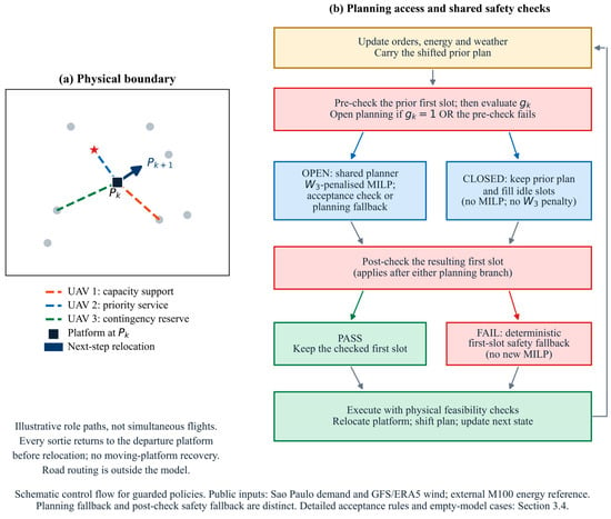
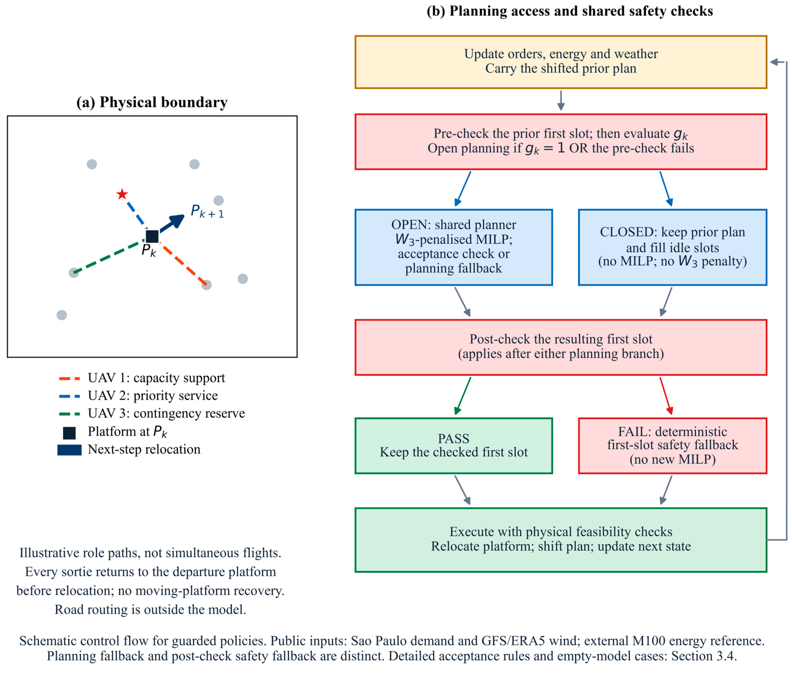
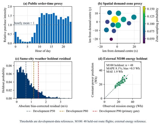
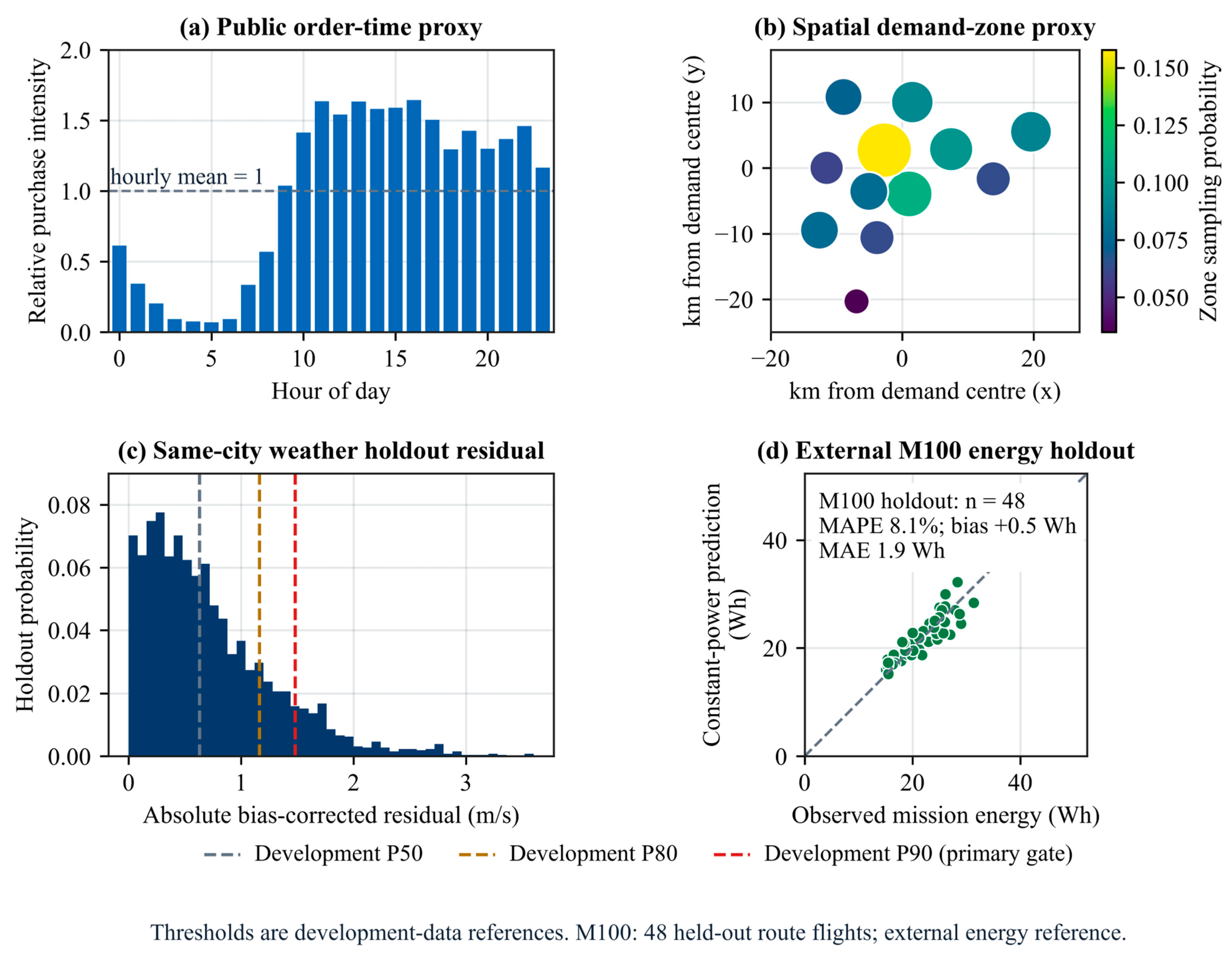
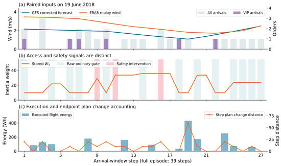
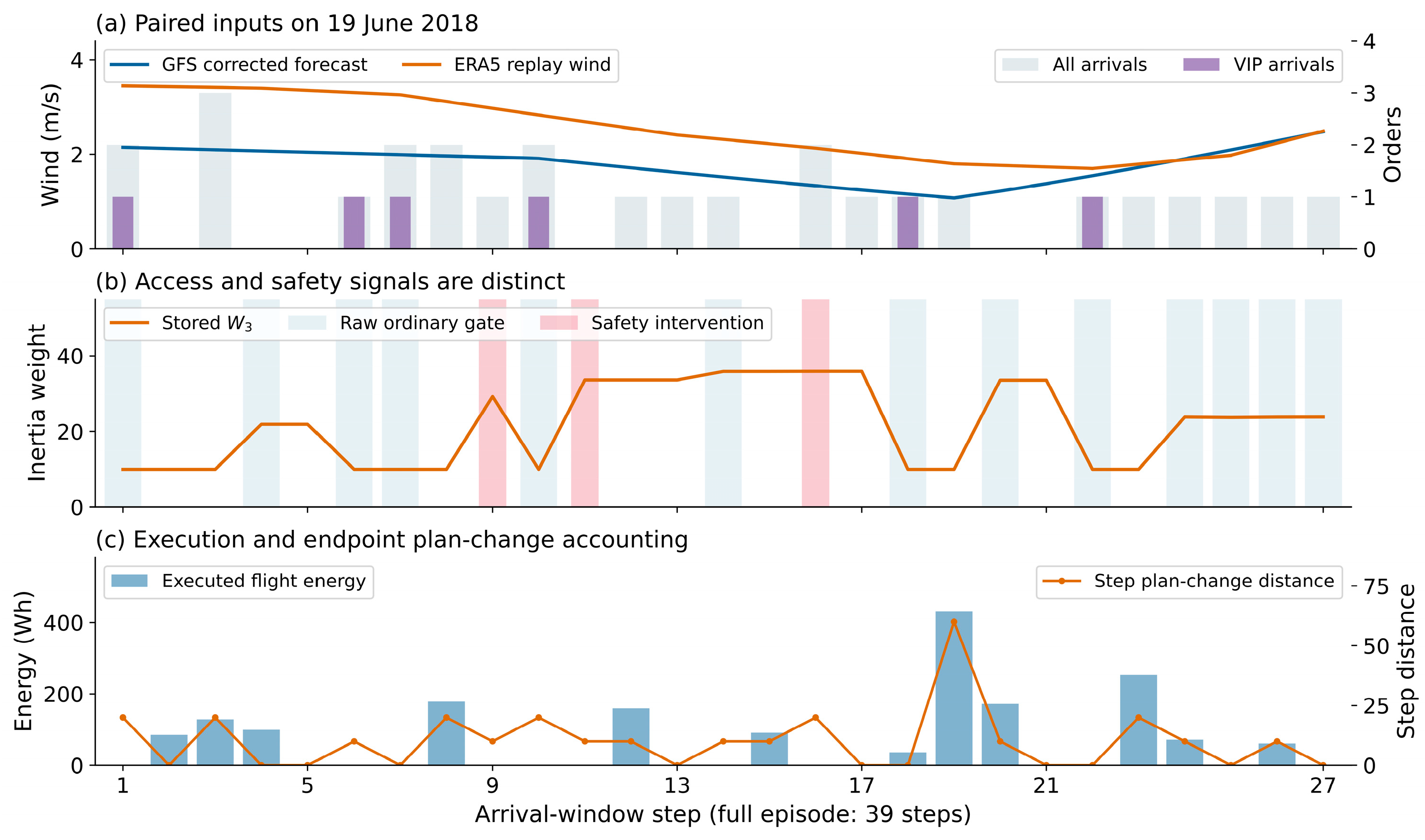
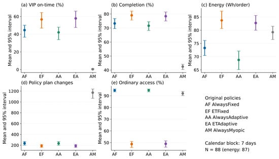
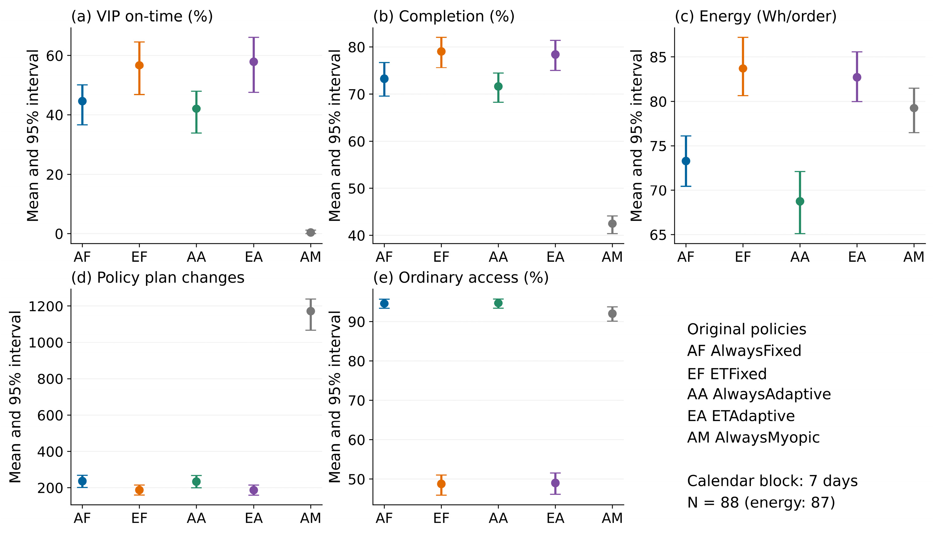
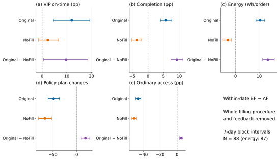
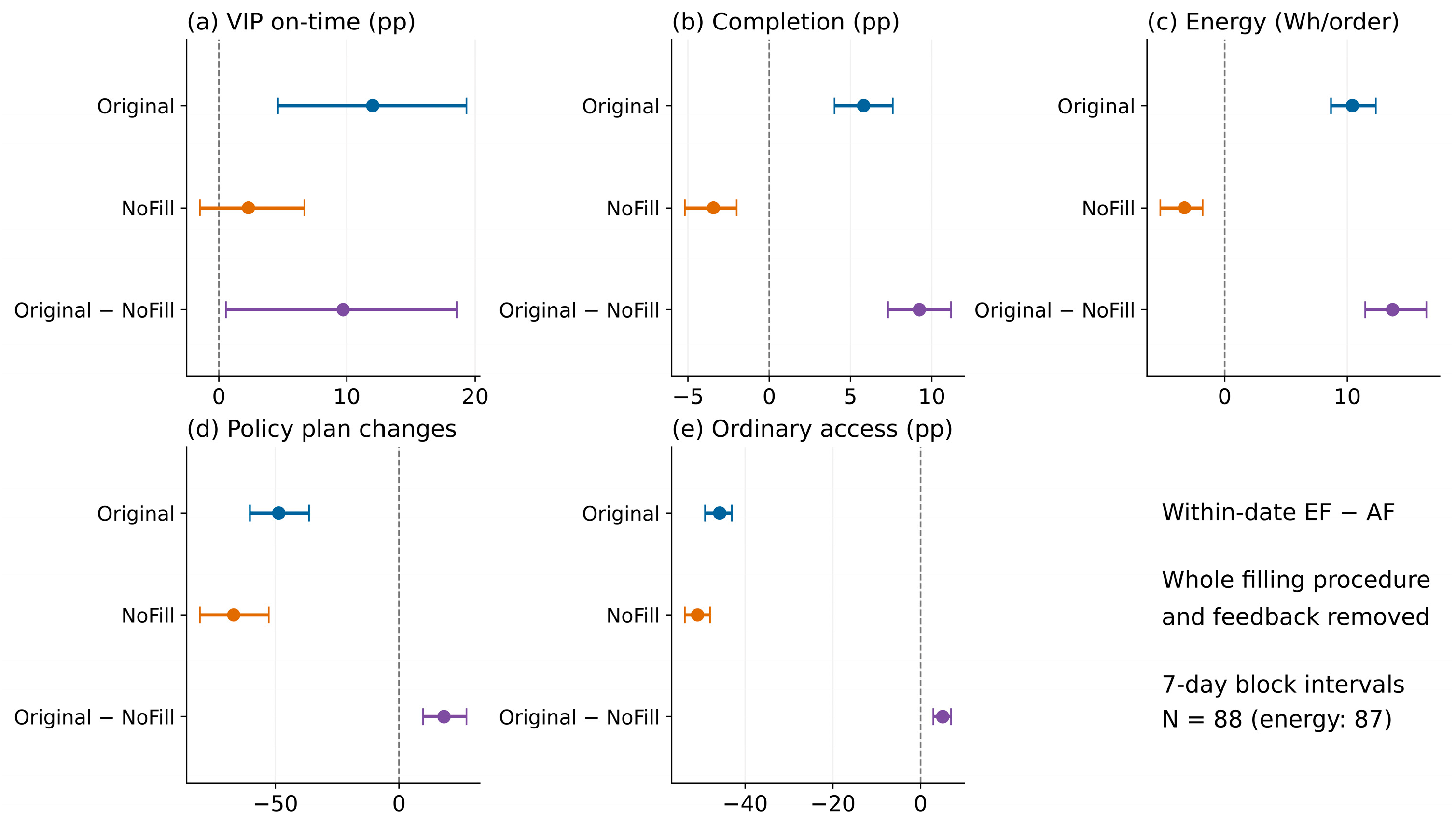
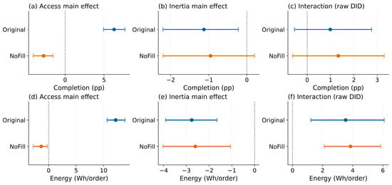
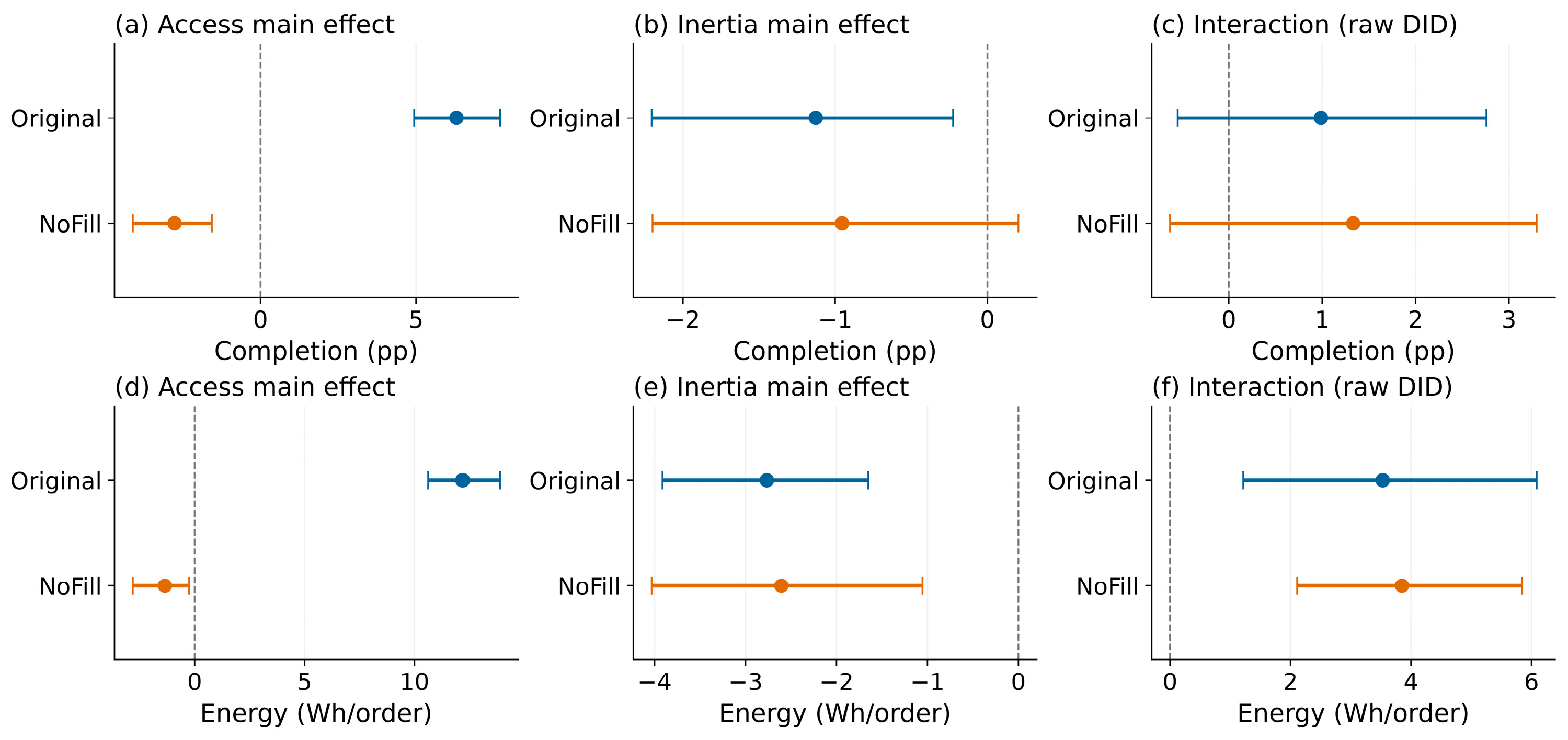
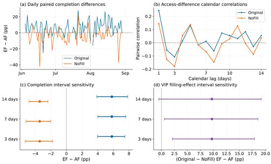
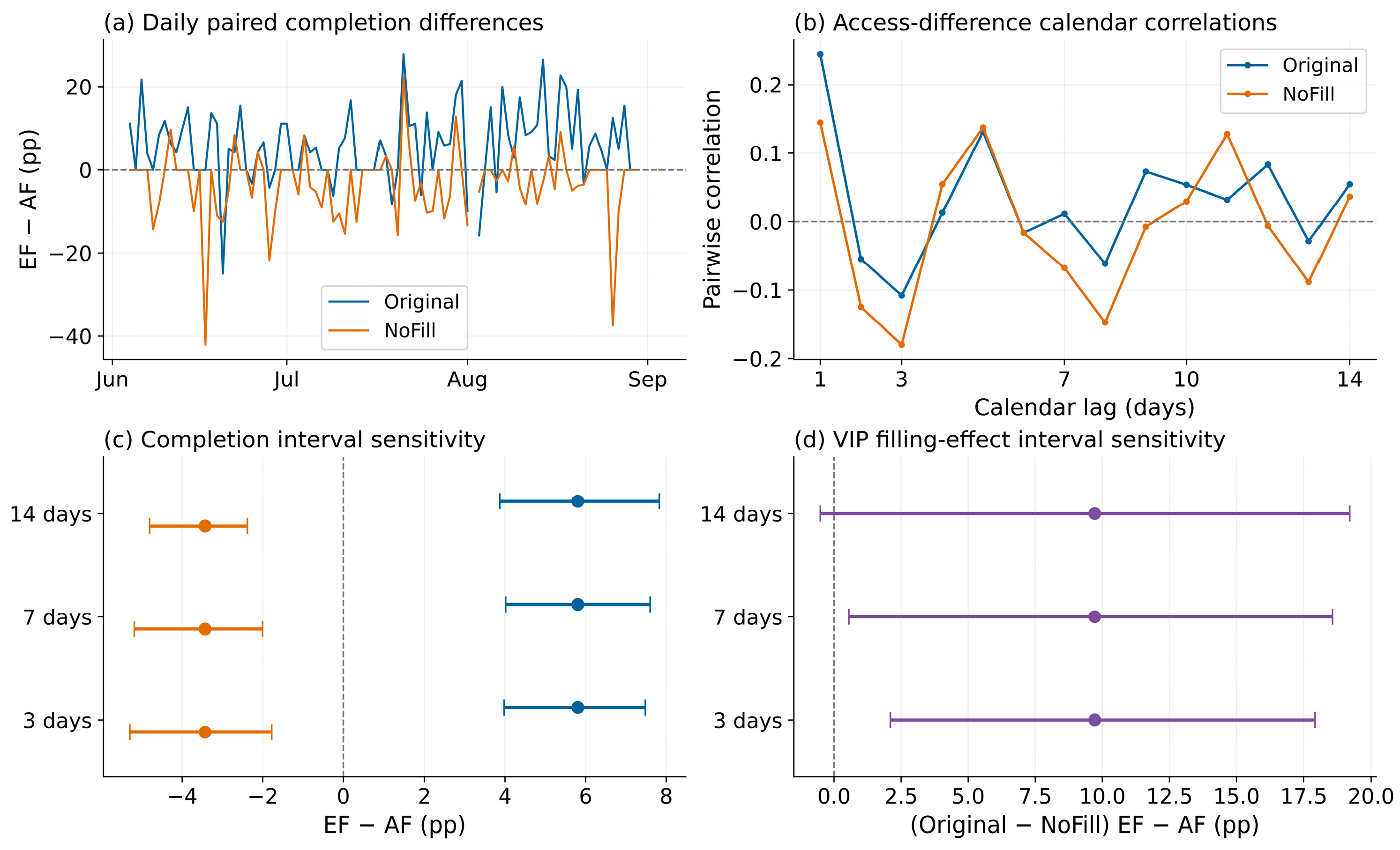

Disclaimer/Publisher’s Note: The statements, opinions and data contained in all publications are solely those of the individual author(s) and contributor(s) and not of MDPI and/or the editor(s). MDPI and/or the editor(s) disclaim responsibility for any injury to people or property resulting from any ideas, methods, instructions or products referred to in the content. |
© 2026 by the authors. Licensee MDPI, Basel, Switzerland. This article is an open access article distributed under the terms and conditions of the Creative Commons Attribution (CC BY) license.