A Replay-Based Big Data Framework for Predictive Maintenance in Industrial IoT

Highlights

Please indicate how your work links to systems science via your contributions to systems practice, theory, and/or methodology.

• A modular Kafka–Spark–LSTM framework integrates data ingestion, distributed stream processing, and AI-based fault prediction for system-level evaluation of predictive maintenance in Industrial IoT.
• A systems-oriented evaluation methodology combines leakage-aware data partitioning with joint assessment of predictive performance, processing latency, throughput, and resource utilization under controlled streaming workloads.

What are the main findings and/or the implications of the main findings?

• The LSTM model achieved 90.4% accuracy, 89.2% precision, 87.6% recall, and an F1-score of 88.4%, outperforming the evaluated threshold-based and Random Forest baselines.
• Under a fixed Kafka–Spark configuration, the framework remained operational at replay loads up to 1.2 million events/min, with observed post-Spark prediction-stage latency ranging from 290 to 570 ms.

Abstract

The rapid growth of Industrial IoT (IIoT) has led to large volumes of sensor data, increasing the need for scalable and data-driven maintenance solutions. This paper presents a replay-based streaming framework for predictive maintenance that integrates Apache Kafka for data ingestion, Apache Spark Streaming for distributed processing, and an LSTM-based model for fault prediction. The NASA CMAPSS FD001 dataset is used in a controlled streaming simulation to evaluate the feasibility of processing multivariate degradation data under different workload levels. To reduce data leakage, engine units are split before sliding-window sequence construction. Experimental results show that the LSTM model achieves 90.4% accuracy, 89.2% precision, 87.6% recall, and an F1-score of 88.4% on the test set. Under the controlled replay conditions, the observed post-Spark prediction-stage latency remained below 600 ms across the evaluated workload levels. Since the Kafka and Spark timing components and the original micro-batch interval were not retained separately, these measurements should not be interpreted as end-to-end pipeline latency. The results demonstrate the feasibility of integrating stream-processing technologies with deep learning for predictive maintenance, while full end-to-end latency and horizontal scalability remain subjects for future evaluation.

1. Introduction

The Industrial Internet of Things (IIoT) has emerged as a transformative force in modern industries by enabling real-time monitoring, automation, and data-driven decision-making [1]. With the deployment of a vast network of interconnected sensors and devices, industries such as manufacturing, energy, and transportation are now able to collect massive volumes of operational data at unprecedented speed and scale. This influx of high-frequency, heterogeneous data opens new avenues for enhancing asset reliability and operational efficiency through intelligent maintenance strategies.

Among these strategies, predictive maintenancehas gained significant attention as it focuses on anticipating equipment failures before they occur [2]. Unlike traditional reactive or preventive maintenance approaches, predictive maintenance leverages data analytics to assess the health of machinery and schedule maintenance only when necessary. This can lead to substantial reductions in downtime, maintenance costs, and production losses. However, realizing predictive maintenance in real-world IIoT environments presents several key challenges.

Firstly, IIoT systems generate data that exhibit the classical 3Vs of big data: volume, velocity, and variety [3]. Processing such data in real time requires architectures that are not only scalable but also capable of handling distributed, low-latency analytics. Secondly, conventional threshold-based or rule-based methods often fall short in identifying early signs of failure, particularly under complex operating conditions. These methods are also prone to high false alarm rates and lack adaptability to changing system dynamics. Thirdly, many existing predictive maintenance solutions operate in batch-processing mode, introducing latency that diminishes their real-time responsiveness.

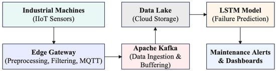
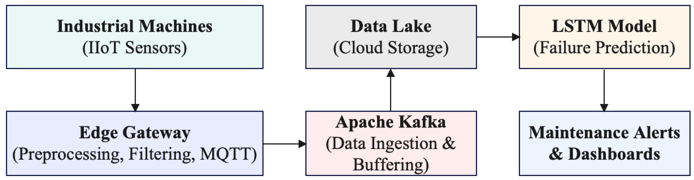
To address these challenges, this paper proposes a big data-driven framework for replay-based predictive maintenance in industrial IoT systems. The framework integrates Apache Kafka for data ingestion, Apache Spark Streaming for distributed micro-batch processing, and a Long Short-Term Memory (LSTM) deep learning model for fault prediction [4]. The NASA CMAPSS dataset, a widely used benchmark in prognostics research, is replayed through a custom streaming pipeline [5] to evaluate predictive performance and workload-dependent system behaviour under controlled simulated loads exceeding one million events per minute. An overview of the proposed system is shown in Figure 1.

Figure 1. Overview of the proposed real-time predictive maintenance system leveraging IIoT, big data technologies, and AI-driven failure prediction.

The main contributions of this paper are summarized as follows:

1.

We design and implement a Kafka–Spark Streaming pipeline for replay-based predictive maintenance using multivariate CMAPSS sensor data.

2.

We integrate an LSTM-based fault prediction model into the streaming pipeline and evaluate its performance against threshold-based and Random Forest baselines.

3.

We define a leakage-aware experimental protocol in which engine units are split before sliding-window construction, ensuring that overlapping windows from the same engine do not appear across training, validation, and test sets.

4.

We evaluate predictive performance and characterize workload-dependent system behaviour under a fixed Kafka–Spark configuration by reporting classification performance, observed post-Spark prediction latency, processed prediction rate, and resource usage under different simulated replay loads.

5.

We provide implementation details, hyperparameters, and the data-splitting protocol to support reproducibility, while explicitly acknowledging that the original Spark micro-batch interval was not retained, which limits exact replication of the streaming timing benchmark.

The remainder of this paper is organized as follows: Section 2 reviews existing literature on predictive maintenance, streaming analytics, and IIoT data processing. Section 3 presents the system architecture and design. Section 4 describes the dataset and simulation environment. Section 5 details the LSTM-based predictive modeling approach. Section 6 provides experimental results and performance evaluations. Section 7 offers a critical discussion on system strengths, limitations, and real-world applicability. Finally, Section 8 concludes the paper and outlines directions for future work. For quick reference, all acronyms used throughout the paper are summarized in Table 1.

Table 1. Table of Acronyms.

Acronym	Definition
IIoT	Industrial Internet of Things
AI	Artificial Intelligence
ML	Machine Learning
DL	Deep Learning
LSTM	Long Short-Term Memory
RNN	Recurrent Neural Network
CNN	Convolutional Neural Network
RUL	Remaining Useful Life
RF	Random Forest
CMAPSS	Commercial Modular Aero-Propulsion System Simulation
ROC	Receiver Operating Characteristic
IoT	Internet of Things
MAPE-K	Monitor–Analyze–Plan–Execute over a Knowledge base

2. Related Work

Predictive maintenance in industrial systems has witnessed substantial progress with the rise of the Industrial Internet of Things (IIoT), big data analytics, and machine learning. This section critically examines the current state of research in three key areas: (1) machine learning-based predictive maintenance, (2) big data platforms for IIoT, and (3) real-time analytics in streaming architectures.

2.1. Predictive Maintenance Using Machine Learning

Machine learning (ML) has become a fundamental approach to predictive maintenance, enabling proactive fault detection and lifecycle optimization [6]. Techniques such as support vector machines (SVM), k-nearest neighbors (KNN), and random forests have shown promise for classifying failure states based on historical sensor trends. More recent studies have adopted deep learning models, including convolutional neural networks (CNNs) and LSTM networks, to capture spatiotemporal patterns in multivariate time-series data [7].

In [8], the authors demonstrated that LSTM models outperform classical classifiers in wind turbine fault prediction tasks, offering enhanced recall and lower false alarm rates. Similarly, in [9], the authors proposed a hybrid CNN-LSTM architecture that achieved state-of-the-art results in rotating machinery fault detection. However, these studies often rely on centralized datasets and assume stable environmental conditions, overlooking critical issues such as communication disruptions, temperature fluctuations, and sensor drift prevalent in desert climates.

2.2. Big Data Platforms for Industrial IoT

To manage the volume, velocity, and variety of IIoT data, researchers have adopted distributed big data frameworks such as Apache Kafka for ingestion, Apache Spark for stream analytics, and Hadoop for storage [10]. These platforms enable scalable analytics pipelines that process millions of events per second across thousands of sensor nodes. A study [11] integrated Hadoop and Spark in a cloud-based predictive maintenance system for industrial robots, achieving real-time performance in high-throughput scenarios.

Nonetheless, such centralized cloud platforms may introduce latency and bandwidth constraints when deployed in large-scale or geographically distributed IIoT environments. Recent advances in edge and fog computing attempt to mitigate this limitation by moving computation closer to the data source [12]. However, the evaluation of complete ingestion-processing-inference pipelines for predictive maintenance remains less developed than model-level prediction studies.

2.3. Real-Time Streaming Architectures

Real-time analytics are crucial in IIoT and smart grid environments where failure response times must be minimized. Stream processing engines such as Apache Flink, Spark Streaming, and Storm support near-real-time data handling with low latency and horizontal scalability. In [13], the authors implemented a Kafka-Flink-based digital twin framework for smart city traffic monitoring, demonstrating dynamic asset control and predictive insights.

However, many streaming-based studies emphasize architectural feasibility without providing sufficient detail on data replay protocols, latency definitions, processing bottlenecks, and reproducibility. This makes it difficult to compare systems fairly or assess whether reported latency and throughput values correspond to model inference only, stream-processing delay, or the complete simulated pipeline [14].

2.4. Research Gaps

Recent studies have increasingly combined IoT architectures with advanced predictive-maintenance models. In [15], an IoT-based framework was proposed using a hybrid CNN–LSTM model on the NASA C-MAPSS FD004 dataset, emphasizing spatial–temporal feature learning and three-class equipment health classification. Similarly, [16] presented an end-to-end IoT analytics architecture integrating Kafka, Spark, InfluxDB, and a modular machine learning pipeline for real-time predictive maintenance. While these studies demonstrate the effectiveness of deep learning and integrated IoT analytics architectures, the present work focuses specifically on the controlled, reproducible evaluation of a Kafka–Spark–LSTM predictive-maintenance pipeline using replayed C-MAPSS FD001 data. In particular, we evaluate both predictive performance and system-level behaviour under varying streaming workloads, including throughput, latency, and resource utilization, while applying an engine-level data-splitting protocol before sequence construction to reduce data leakage.

Although predictive maintenance using machine learning and deep learning has been widely studied, several limitations remain in the evaluation of real-time predictive maintenance pipelines. First, many studies primarily emphasize model-level predictive performance, such as accuracy, precision, recall, and F1-score, while comparatively less attention is given to the behaviour of the complete streaming pipeline under varying workloads [17]. Consequently, evaluating predictive accuracy alone may not sufficiently demonstrate whether a predictive maintenance framework can maintain responsive processing under high-frequency IIoT workloads [18]. A more comprehensive evaluation should therefore consider predictive performance together with ingestion throughput, processing latency, and resource utilization.

Second, benchmark datasets such as NASA CMAPSS are commonly used for prognostics research, but they are offline datasets rather than streaming-native data sources. When such datasets are replayed to emulate streaming conditions, the replay protocol, timestamp generation, windowing strategy, and data-splitting procedure must be clearly defined to avoid unrealistic assumptions and data leakage [6].

Third, existing studies often report aggregate latency or accuracy values without separating the contributions of the ingestion layer, stream-processing layer, and model-inference layer. As a result, the actual bottleneck in the pipeline remains unclear. A rigorous evaluation should therefore clearly define the timing boundaries associated with Kafka ingestion, Spark Streaming processing, model inference, and overall pipeline responsiveness [10].

Finally, reproducibility remains a recurring limitation in predictive maintenance studies that combine streaming platforms and deep learning models. Details such as random seeds, train–validation–test splits, sliding-window construction, hyperparameters, hardware configuration, and experimental settings are essential for allowing other researchers to reproduce and verify the reported results [14].

Based on these gaps, this study presents a replay-based predictive maintenance framework integrating Kafka, Spark Streaming, and an LSTM model using C-MAPSS FD001 sensor data. The contribution is not a new deep-learning architecture; rather, the study provides a controlled evaluation of predictive performance and streaming-system behaviour, together with an engine-level data-splitting protocol designed to reduce data leakage and clearly documented experimental settings to improve reproducibility.

3. System Architecture

The proposed framework is a replay-based big data pipeline designed to evaluate predictive maintenance under controlled Industrial IoT (IIoT)-style streaming conditions. It integrates Apache Kafka for data ingestion, Apache Spark Streaming for distributed stream processing, and an LSTM-based deep learning model for time-series fault prediction.

3.1. Overview

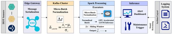
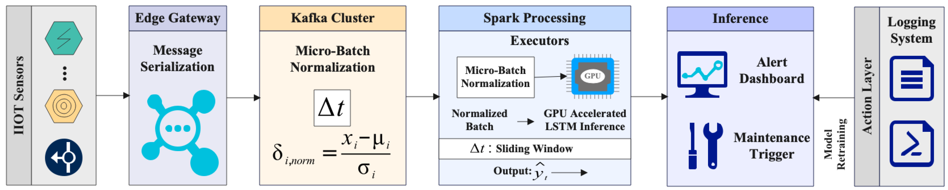
Figure 2 illustrates the proposed system architecture, which integrates components for buffered data ingestion, distributed micro-batch processing, and model-based fault prediction in Industrial IoT (IIoT)-style environments. The architecture consists of five key stages: (1) Edge Device Layer, (2) Kafka Ingestion Pipeline, (3) Spark Streaming and Preprocessing Engine, (4) Deep Learning Inference with LSTM, and (5) action layer for dashboard alerts and retraining feedback.

Figure 2. System architecture for real-time predictive maintenance using edge IoT devices, Kafka, Spark, and LSTM.

At the edge layer, diverse IIoT sensors (e.g., temperature, vibration, pressure, RPM) continuously monitor equipment conditions. These signals are first passed through local preprocessing units, responsible for denoising, timestamping, and feature encoding, and forwarded via MQTT to nearby edge gateways. Edge nodes optionally filter redundant events to reduce upstream traffic.

In the Kafka layer, the preprocessed data is ingested into partitioned topics with fault-tolerant replication. Kafka acts as a distributed buffer, ensuring decoupling between data producers (sensors) and consumers (stream processors). Kafka’s partitioned architecture and ordering guarantees provide mechanisms for supporting high-throughput data ingestion. However, the effect of horizontally scaling Kafka partitions or brokers was not empirically evaluated in the present study.

The real-time analytics layer uses Apache Spark Streaming to consume micro-batches from Kafka. Each batch is processed within a sliding window $\Delta t$, normalized, and transformed into temporal sequences for model input. Preprocessing includes statistical smoothing, missing-value imputation, and feature scaling. Spark’s Resilient Distributed Datasets (RDDs) [19] enable parallel transformation and low-latency computation.

The prediction engine applies an LSTM neural network trained on historical failure patterns. It forecasts degradation trends and failure probabilities ${\widehat{y}}_t$ using multi-sensor sequences. If the prediction exceeds a predefined fault threshold $\theta$, an alert is generated. The model is containerized using Docker for GPU-enabled inference and can be retrained periodically from recent streaming data.

Finally, the action layer logs alerts, visualizes system status on a dashboard, and forwards anomalies to maintenance teams. A feedback loop exists between the action layer and the model trainer to support online retraining and model drift correction.

Architecturally, Kafka partitions, Spark executors, edge nodes, and containerized inference components can be deployed in parallel across clusters [20]. However, the present experiments use a fixed Kafka–Spark configuration and therefore do not empirically demonstrate horizontal scalability or large-scale industrial deployment readiness.

3.2. Data Ingestion with Apache Kafka

Industrial equipment typically generates high-frequency, heterogeneous sensor data streams including temperature, vibration, pressure, and rotational speed. These streams, denoted as ${\mathbf{X}}_t=\{x_1^t,x_2^t,\dots ,x_n^t\}$, are timestamped and encoded as message payloads for ingestion into the big data pipeline. Each $x_i^t$ represents the value of sensor i at time t, and the overall stream ${\mathbf{X}}_t$ captures the system state at that moment.

Apache Kafka serves as the primary data ingestion backbone due to its high throughput, distributed architecture, and strong delivery guarantees. Kafka organizes incoming sensor data into topics, each of which can be logically mapped to a machine, subsystem, or sensor type. Topics are further partitioned to enable parallel consumption and horizontal scaling.

Messages are ingested and written to Kafka’s distributed commit log. Each partition is an ordered, immutable sequence of records that supports append-only writes. Kafka ensures durability through replication: each partition is replicated R times across brokers to guard against node failures. The data ingestion throughput can be estimated as:

$$T_{\mathrm{kafka}}=P·R·B_m$$

(1)

where P is the number of partitions, R is the replication factor, and $B_m$ is the message bandwidth per broker (in bytes/sec).

Kafka’s design enables time-decoupled producer-consumer interaction. Producers (e.g., edge sensor gateways) push real-time data to Kafka, while consumers (e.g., Spark Streaming jobs) pull data in mini-batches. This decoupling makes the architecture resilient to processing backlogs and supports reliable buffering during temporary downstream outages [21].

Each Kafka message includes a key, value, and timestamp. In the simulated replay setup, preprocessed CMAPSS records are published as timestamped sensor events to Kafka topics. The producer controls the replay rate to emulate different workload levels, allowing the pipeline to be evaluated under low, medium, and high event-rate conditions.

Kafka’s retention and buffering mechanisms support replay-based testing and temporary decoupling between producers and consumers [22]. In this study, Kafka is used as the ingestion and buffering layer in a controlled simulation, rather than as evidence of a fully deployed industrial fault-tolerant system.

3.3. Real-Time Processing with Apache Spark Streaming

Apache Spark Streaming forms the core real-time analytics layer of the proposed system. It continuously processes incoming Kafka data streams in micro-batches, enabling near real-time monitoring and transformation of sensor data. Spark supports distributed parallelism using RDDs and structured streaming APIs and provides mechanisms for fault-tolerant processing across multiple executors. However, the Spark configuration was fixed in the present experiments, and horizontal scalability was not empirically evaluated.

Each Kafka topic feed is subscribed to by a Spark Streaming job configured with a micro-batch interval $\Delta t$. The exact micro-batch interval used in the reported experimental runs was not retained in the experimental logs and is therefore acknowledged as a reproducibility limitation of the present study. During each interval, messages arriving from all partitions are aggregated into an RDD representing the input data block for that batch:

$$D_{\Delta t}={\displaystyle \bigcup _{i=1}^n}\left\{x_i^{t-\Delta t},\dots ,x_i^t\right\}$$

(2)

Here, $x_i^t$ denotes the sensor value for feature i at time t, and $D_{\Delta t}$ encapsulates the entire feature stream window across all n sensors.

For the experiments reported in this study, sensor features are normalized using min–max scaling rather than sliding-window standardization. To prevent information leakage, the minimum and maximum values for each retained feature are computed exclusively from the training data and subsequently applied unchanged to the validation, test, and replayed streaming data. The normalized value of feature i is calculated as:

$$x_i^{t,\mathrm{norm}}={\displaystyle \frac{x_i^t-x_i^{min,\mathrm{train}}}{x_i^{max,\mathrm{train}}-x_i^{min,\mathrm{train}}}}$$

(3)

where $x_i^{min,\mathrm{train}}$ and $x_i^{max,\mathrm{train}}$ denote the minimum and maximum values of feature i obtained from the training data. Using fixed training-derived scaling parameters ensures consistent preprocessing across the training, validation, test, and replayed streaming samples while avoiding information leakage.

Spark Streaming pipelines are defined as a directed acyclic graph (DAG) of operations such as ‘map’, ‘filter’, and ‘reduce’ [23]. For example, an anomaly score can be generated in each micro-batch using a custom ‘UDF()’ (user-defined function), and maintenance alerts are pushed downstream based on LSTM predictions exceeding a risk threshold $\theta$.

Each Spark executor handles a partition of the batch RDD and performs computations in parallel, enabling parallel processing across the available executors. The present experiments did not vary the number of executors or cores and therefore do not quantify horizontal or linear scalability.

Spark Streaming also supports structured streaming for more declarative processing. This approach allows stateful operations (e.g., event-time windowed aggregations and joins across data streams) and provides exactly-once processing semantics, critical for applications requiring strong consistency guarantees in industrial maintenance pipelines.

3.4. LSTM-Based Predictive Model

The final stage in the system pipeline is a deep learning module that predicts equipment degradation or imminent failure based on time-series sensor patterns. LSTM networks are particularly suitable for this task due to their ability to learn long-term dependencies in sequential data, mitigate vanishing gradients, and preserve temporal context.

Let $\mathbf{X}=\{x_t,x_{t+1},\dots ,x_{t+k}\}$ represent the input window of normalized sensor readings. Each vector $x_t\in {\mathbb{R}}^d$ encodes d features observed at time t. The LSTM cell maintains two internal states: the hidden state $h_t$ and the cell memory $c_t$. At each time step, the LSTM updates these using input, forget, and output gates, as shown in Equation (4a)–(4e).

$$\begin{array}{cc}\hfill f_t& =\sigma (W_f{x}_t+U_f{h}_{t-1}+b_f)\hfill \end{array}$$

(4a)

$$\begin{array}{cc}\hfill i_t& =\sigma (W_i{x}_t+U_i{h}_{t-1}+b_i)\hfill \end{array}$$

(4b)

$$\begin{array}{cc}\hfill o_t& =\sigma (W_o{x}_t+U_o{h}_{t-1}+b_o)\hfill \end{array}$$

(4c)

$$\begin{array}{cc}\hfill c_t& =f_t\odot c_{t-1}+i_t\odot tanh(W_c{x}_t+U_c{h}_{t-1}+b_c)\hfill \end{array}$$

(4d)

$$\begin{array}{cc}\hfill h_t& =o_t\odot tanh\left(c_t\right)\hfill \end{array}$$

(4e)

Here, $\sigma$ denotes the sigmoid activation function, ⊙ is the element-wise (Hadamard) product, and $W_{*}$, $U_{*}$, and $b_{*}$ are learnable weights and biases of the LSTM cell for the respective gates.

After processing the full sequence, the last hidden state $h_{t+k}$ encapsulates the learned temporal context. A dense output layer computes the final prediction ${\widehat{y}}_t$, representing the estimated failure risk or Remaining Useful Life (RUL):

$${\widehat{y}}_t=\sigma (W_y{h}_{t+k}+b_y)$$

(5)

where $W_y$ and $b_y$ are parameters of the final regression/classification layer. The sigmoid activation bounds ${\widehat{y}}_t\in [0,1]$, suitable for binary classification of failure/no-failure, or thresholded regression-based alerting.

The model is trained using backpropagation through time (BPTT) [24] with the binary cross-entropy loss function used for the binary failure-classification task. During inference, a decision threshold of $\theta =0.5$ is used to convert the predicted failure probability into the binary failure/no-failure classification used in the reported experiments.

To support streaming inference, the trained LSTM model is deployed as part of the simulated processing pipeline. The model receives normalized fixed-length sequences generated from each micro-batch and outputs a failure probability for threshold-based alerting.

To ensure modularity and clarity in deployment, the end-to-end pipeline is implemented as a streaming loop consisting of Kafka ingestion, Spark-based normalization, LSTM prediction, and threshold-based alerting. This pipeline is outlined in Algorithm 1, where each incoming batch ${\mathbf{X}}_t$ is normalized and evaluated by the LSTM model. Maintenance alerts are triggered when the predicted failure risk ${\widehat{y}}_t$ exceeds a defined threshold $\theta$, enabling threshold-based alert generation within the simulated streaming pipeline.

Algorithm 1 Real-Time Predictive Maintenance Pipeline

1: Initialize KafkaConsumer, SparkSession, LSTMModel 2: while True do 3:     ${\mathbf{X}}_t\leftarrow$ Read from Kafka 4:     ${\mathbf{X}}_t^{\mathrm{norm}}\leftarrow$ Normalize$\left({\mathbf{X}}_t\right)$ 5:     ${\widehat{y}}_t\leftarrow$ LSTMModel.predict(${\mathbf{X}}_t^{\mathrm{norm}}$) 6:     if ${\widehat{y}}_t>\theta$ then 7:         Trigger Maintenance Alert 8:     end if 9: end while

3.5. Architectural Scaling and Latency Considerations

The proposed architecture is designed to support distributed processing and low-latency prediction. However, the present study evaluates workload-dependent behaviour under a fixed Kafka–Spark configuration and does not empirically assess horizontal scalability.

• Kafka Layer: Kafka supports partition-based parallelism and can be configured with multiple brokers. Increasing the number of partitions can increase the available ingestion parallelism, although the realized throughput depends on the broker, producer, consumer, network, and hardware configuration. The effect of varying Kafka partitions or brokers was not evaluated in the present experiments.
• Spark Streaming Layer: Apache Spark Streaming employs a micro-batch model, where jobs are distributed to multiple executors. Each executor processes a subset of the RDD, enabling parallel computation. This supports elasticity in computational resources, as new nodes can be dynamically added or removed without disrupting streaming pipelines.
• Inference Layer: The trained LSTM model receives normalized fixed-length sequences and generates failure-probability scores. The inference layer can be scaled in future deployments, but the present study evaluates it within a controlled replay-based simulation.

Conceptually, the overall pipeline latency can be decomposed into the latency introduced by the ingestion, stream-processing, and inference stages:

$$L=L_{\mathrm{ingest}}+L_{\mathrm{batch}}+L_{\mathrm{inference}}$$

(6)

where:

• $L_{\mathrm{ingest}}$ is the time taken by Kafka to receive, partition, and buffer messages.
• $L_{\mathrm{batch}}$ is the time for Spark to collect, process, and transform each micro-batch.
• $L_{\mathrm{inference}}$ is the runtime required to make predictions using the LSTM model.

For the reported experiments, however, these latency components were not instrumented separately. The measured metric is defined as application-level processing latency within the controlled Kafka–Spark replay pipeline. The timing starts when a processed Spark micro-batch becomes available for model inference and ends when the corresponding LSTM prediction output is generated. Consequently, the reported latency does not represent physical sensor-to-cloud end-to-end latency and does not separately quantify Kafka queueing/broker delay, Spark scheduling and processing time, or standalone LSTM inference time.

Spark Streaming operates using a configurable micro-batch interval $\Delta t$, as described in Section 3.3. Queueing time and the individual processing contributions of Kafka, Spark, and the LSTM were not independently recorded in the present experiment; a fully instrumented component-level latency analysis is therefore left for future work.

In the present controlled experiments, workload response was evaluated by varying the incoming event rate while keeping the underlying Kafka–Spark configuration fixed. Therefore, the reported results characterize the framework’s response to increasing workload rather than empirical horizontal scalability. Evaluation of horizontal scaling by varying Kafka partitions, brokers, Spark executors, and computational resources is left for future work.

4. Dataset and Simulation Setup

To evaluate the proposed real-time predictive maintenance framework, we use the NASA CMAPSS (Commercial Modular Aero-Propulsion System Simulation) dataset [5], a well-established benchmark in the prognostics and health management (PHM) domain. The dataset simulates degradation in aircraft turbofan engines and provides multivariate time-series data capturing sensor readings over time until failure.

4.1. NASA CMAPSS Dataset

The CMAPSS dataset comprises four sub-datasets, each representing different operating and fault conditions. Each record corresponds to a single engine unit and includes a sequence of operational cycles until a failure occurs. At each cycle, 21 sensor measurements and 3 operational settings are recorded. These measurements include critical variables such as fan speed, pressure ratios, temperatures, and vibration signals.

In this study, we use the FD001 subset, which contains data from 100 engine units operating under consistent flight conditions and single fault modes [25]. This subset provides sufficient complexity for evaluating temporal degradation patterns while ensuring reproducibility. Each unit’s life ends in a failure, allowing supervised learning of remaining useful life (RUL) and early fault prediction.

4.2. Data Preprocessing

Before streaming the data, several preprocessing steps are performed:

• Normalization: All sensor readings are normalized using min–max scaling to improve convergence during model training.
• Smoothing and Feature Selection: Feature selection is performed exclusively on the training partition to avoid information leakage. Near-constant and redundant sensor signals are excluded based on variance and pairwise correlation analysis, while informative sensor features exhibiting meaningful degradation-related variation are retained. The resulting feature-selection mask is then applied unchanged to the validation, test, and replayed streaming data.
• Labeling: For supervised learning, the remaining useful life (RUL) is computed for each cycle. Binary labels are assigned to indicate proximity to failure within a predefined prediction window.
• Sequence Construction: For LSTM modeling, each engine’s data is segmented into overlapping time windows (e.g., sequences of 30 cycles) to capture temporal dependencies.

To ensure that feature selection does not benefit from information contained in the validation or test partitions, the variance and correlation analysis is fitted using the training data only. The identified feature set is subsequently fixed for all remaining experimental stages.

In the reported experiments, these preprocessing steps were performed offline before the data were replayed through the Kafka–Spark Streaming pipeline. Therefore, the streaming performance measurements reported in this study are based on preprocessed and sequence-constructed input data, and the computational time required for offline preprocessing is not included in the reported streaming latency. Consequently, the reported latency excludes offline preprocessing and should be interpreted as post-Spark prediction-stage latency rather than end-to-end Kafka–Spark–LSTM pipeline latency.

4.3. Real-Time Streaming Simulation

Since the original CMAPSS dataset is static, we simulate a real-time industrial environment by replaying the dataset through a custom-built IoT streaming pipeline.

• Data Ingestion with Kafka: The preprocessed time-series records are published as sensor events to Apache Kafka topics, mimicking high-frequency telemetry streams from distributed edge devices.
• Stream Processing with Spark: Kafka serves as the input stream for Apache Spark Streaming, which processes the data in near real-time micro-batches. Spark transforms the streaming records into feature vectors and feeds them into the deployed LSTM model for inference.
• Throughput Control: To emulate industrial workloads, the replay engine dynamically controls the publishing rate to Kafka, achieving up to one million sensor events per minute.
• Visualization and Logging: Real-time dashboards (Grafana) are used to visualize prediction outputs, system latency, and throughput metrics.

This simulation framework provides a controlled environment for evaluating predictive performance and workload-dependent behaviour under replayed streaming conditions. The results should therefore be interpreted as controlled simulation evidence rather than as validation against production Industry 4.0 operational requirements.

4.4. Experimental Environment

The experiments were conducted using a controlled replay-based Kafka–Spark environment rather than a production IIoT deployment. Apache Kafka was used for replay-based data ingestion, Apache Spark Streaming for micro-batch stream processing, and the trained LSTM model for fault prediction. The available hardware, software, and streaming configuration details used in the experimental environment are summarized in Table 2.

Table 2. Experimental Environment and Streaming Configuration.

Parameter	Configuration
Hardware	8-core Intel Core i7 CPU, 16 GB RAM, CPU-based inference
Operating system	Ubuntu 22.04 LTS (64-bit)
Apache Kafka version	Apache Kafka 3.6.1
Apache Spark version	Apache Spark 3.5.0
Deep-learning framework	TensorFlow 2.15/Keras
Kafka brokers	1 broker
Kafka partitions	4 partitions
Replication factor	1
Spark executors	2 executors
Executor cores	2 cores per executor
Micro-batch interval	Not retained in the experimental logs
Deployment topology	Single-machine controlled replay-based Kafka–Spark environment

5. Predictive Modeling

This section describes the deep learning model used for real-time predictive maintenance, focusing on the design, training, and deployment of an LSTM network for forecasting equipment faults from multivariate time-series sensor data.

5.1. LSTM Modelling Considerations

The LSTM model is used to capture temporal degradation patterns from multivariate sensor sequences and to estimate the likelihood of an impending equipment failure. Its recurrent structure enables information from previous time steps to influence subsequent predictions, which is important when degradation develops progressively across multiple operating cycles.

Despite these advantages, LSTM networks also have limitations. Although their gating mechanisms improve the modelling of long-term dependencies, performance can still deteriorate for very long sequences, and their recurrent structure and multiple gating operations introduce additional computational and training overhead [26]. These considerations are particularly important for real-time predictive maintenance, where predictive performance must be balanced against inference latency and available computational resources.

5.2. Model Architecture

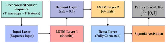
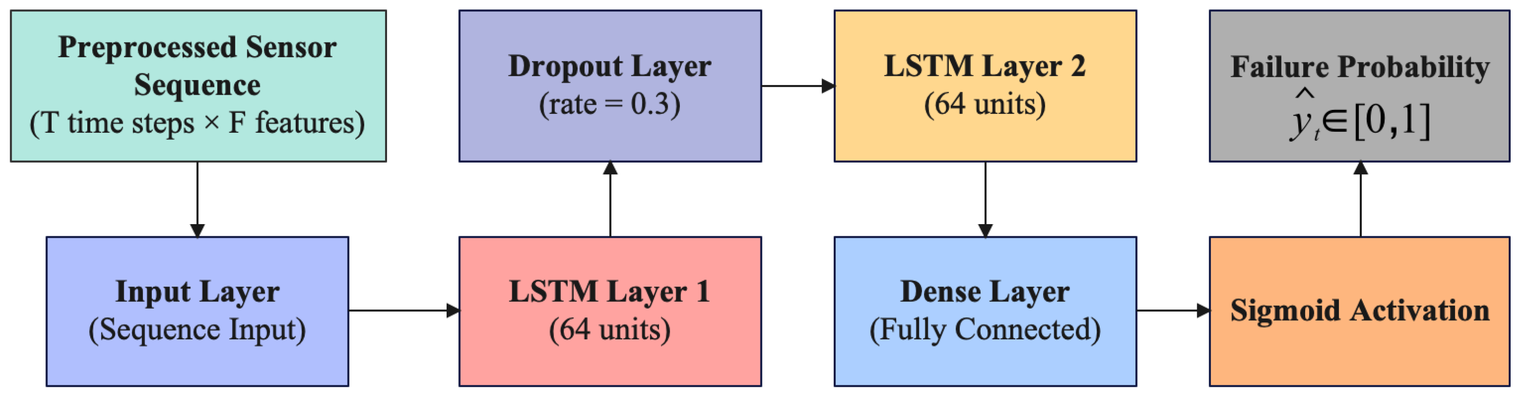
The LSTM model is trained to perform binary classification, predicting whether an equipment failure is likely to occur within a fixed prediction window. The architecture consists of the following components:

• Input Layer: Accepts sequences of sensor readings, each of length T time steps and F features per step.
• LSTM Layers: Two stacked LSTM layers with 64 hidden units each are used to capture temporal dependencies across sensor sequences.
• Dropout Layer: A dropout rate of 0.2 is applied to reduce overfitting.
• Dense Layer: A fully connected layer followed by a sigmoid activation function for binary classification output.

The model is trained using the binary cross-entropy loss function [27] and the Adam optimizer [28]. Early stopping and learning rate scheduling are employed to prevent overfitting and optimize convergence. The architecture of the LSTM-based predictive model is illustrated in Figure 3.

Figure 3. Architecture of the LSTM-based predictive model. The input consists of preprocessed multivariate time-series data with T time steps and F features. Two stacked LSTM layers (64 units each) capture temporal dependencies, followed by a dense layer and sigmoid activation to output failure probability ${\widehat{y}}_t\in [0,1]$.

5.3. Training Setup

The LSTM model was trained offline using historical sequences from the NASA CMAPSS FD001 subset before being deployed in the simulated streaming inference pipeline. To avoid data leakage, the dataset was first divided at the engine-unit level before any sliding-window sequence construction was applied. Specifically, the 100 engine units in FD001 were divided into 70 engines for training, 15 engines for validation, and 15 engines for testing. This engine-wise split ensures that overlapping windows generated from the same engine trajectory do not appear across training, validation, and test sets.

Each input sample was constructed using a sliding window of length $T=30$ cycles over the run-to-failure trajectory of an engine unit. The binary target label indicates whether a failure is expected within the next $n=20$ cycles, making the task suitable for early fault prediction. Since the sliding windows were generated only after the engine-level split, the number of test samples is larger than the number of test engines, while still preserving separation between training and test trajectories.

Sensor readings were normalized using statistics computed from the training set and then applied consistently to the validation and test sets. The LSTM model was trained using binary cross-entropy loss and the Adam optimizer. Dropout was applied to reduce overfitting, and validation loss was monitored during training to select the final model configuration.

To further support reproducibility, the main implementation settings and hyperparameters used in the controlled experiment are summarized in Table 3. The reported classification results are based on a single controlled experimental run using the reserved test engines. Therefore, the results should be interpreted as the outcome of one fixed train–validation–test protocol rather than averages over repeated independent runs or cross-validation folds.

Table 3. Implementation Details and Hyper-parameters.

Parameter	Setting
Dataset	NASA CMAPSS FD001
Number of engine units	100 engines
Data split	70 training engines, 15 validation engines, 15 test engines
Leakage prevention	Engine-wise split performed before sliding-window construction
Sequence length	$T=30$ cycles
Prediction window	$n=20$ cycles
Input features	Selected and normalized multivariate sensor readings
Feature selection	Correlation-based removal of noisy or redundant sensor signals
Normalization	Min–max scaling fitted on the training set and applied to validation and test sets
Model architecture	Two stacked LSTM layers with 64 hidden units each, followed by dropout and a dense sigmoid output layer
Loss function	Binary cross-entropy
Optimizer	Adam
Learning rate	$0.001$
Batch size	64
Dropout rate	0.2
Training epochs	10
Early stopping criterion	Validation loss monitoring with best validation model retained
Random seed	42
Number of experimental runs	Single controlled run
Evaluation setting	Reserved test engines only
Streaming setup	Replay-based Kafka–Spark simulation using preprocessed CMAPSS records
Latency definition	Application-level simulated pipeline latency, not physical sensor-to-cloud latency

5.4. Model Deployment in Streaming Pipeline

After training, the LSTM model is deployed within the Spark Streaming pipeline for real-time inference. Each micro-batch of incoming sensor events is grouped by engine ID and converted into fixed-length sequences using windowing operations. These sequences are then passed through the model to produce fault probability scores in real time.

For the reported experimental results, a decision threshold of $\theta =0.5$ was used to convert the predicted failure probability into the final binary classification. A sequence with a predicted failure probability greater than or equal to 0.5 is classified as a failure case and triggers a maintenance alert; otherwise, it is classified as normal. These alerts are logged and visualized using real-time dashboards, enabling operators to act proactively.

5.5. Baseline Comparison

To evaluate the effectiveness of the proposed LSTM model, we compare its performance against two baseline methods:

• Threshold-Based Rules: Simple rules based on sensor thresholds, widely used in traditional maintenance systems [29].
• Random Forest Classifier: A static, non-sequential model trained on aggregated statistical features (mean, std, etc.) from the sensor time windows [30].

As shown in Section 6, the LSTM model achieves higher predictive performance than the evaluated baseline methods across the reported classification metrics.

6. Experimental Results

This section presents a comprehensive evaluation of the proposed predictive maintenance framework under controlled replay conditions. We assess the prediction accuracy of the LSTM model, the system’s workload-dependent behaviour, comparisons with baseline methods, and the resource utilization of the pipeline under different simulated replay loads.

6.1. Evaluation Metrics

To assess the performance of the proposed LSTM-based predictive maintenance model, the test set was constructed from the 15 engine units reserved during the engine-wise train–validation–test split. The split was performed before sliding-window construction to prevent leakage of overlapping temporal windows across different data partitions. Therefore, although the FD001 subset contains 100 engine units, the final number of test instances is larger than 15 because multiple overlapping sequences are generated from each test engine trajectory.

The evaluation considered both predictive performance and simulated streaming responsiveness. Predictive performance was measured using accuracy, precision, recall, F1-score, ROC-AUC, and confusion matrix analysis. Streaming responsiveness was measured as the application-level processing latency observed in the simulated Kafka–Spark replay pipeline. In this study, latency refers to the elapsed time between the availability of a processed micro-batch for inference and the generation of the corresponding prediction output. It should therefore be interpreted as simulated pipeline latency rather than a direct measurement of physical sensor-to-cloud industrial latency. The following metrics were used to quantify performance:

• Accuracy: Measures the overall correctness of predictions, computed as the ratio of correctly predicted instances (both failure and non-failure) to the total number of predictions.
• Precision: Indicates the proportion of correctly predicted failure instances among all instances predicted as failure. A high precision value suggests low False Positive Rates, which is critical in reducing unnecessary maintenance costs.
• Recall: Represents the proportion of actual failure instances that were correctly predicted by the model. High recall ensures that imminent failures are not overlooked, reducing the risk of unexpected breakdowns.
• F1-Score: Provides a balanced measure by calculating the harmonic mean of precision and recall. It is particularly useful when there is a trade-off between false positives and false negatives.
• Latency: Captures the application-level time observed in the simulated Kafka–Spark replay pipeline for processing a micro-batch and generating the corresponding prediction output.

Table 4 summarizes the results obtained using the proposed model. The LSTM network achieved a high accuracy of 90.4%, with strong precision and recall values of 89.2% and 87.6%, respectively. The F1-score of 88.4% demonstrates a strong balance between detecting true failures and minimizing false alarms. The average processing latency was measured at 412 milliseconds, supporting the feasibility of the proposed framework under controlled simulated streaming conditions. These results demonstrate the predictive performance of the model and the observed post-Spark prediction-stage latency under the controlled replay conditions evaluated in this study. All performance values reported in Table 4 correspond to this single controlled test run and are not reported as mean values over repeated runs.

Table 4. Prediction Metrics on Test Dataset.

Metric	Value
Accuracy	90.4%
Precision	89.2%
Recall	87.6%
F1-Score	88.4%
Average Processing Latency	412 ms

6.2. Training and Convergence Behavior

To evaluate the convergence stability and learning dynamics of the LSTM model, we monitored the binary cross-entropy (BCE) loss on both the training and validation sets across 10 training epochs.

As shown in Table 5, the training loss consistently decreased with each epoch, starting at 0.0912 and reaching 0.0375 by epoch 10. This indicates that the model effectively learned patterns from the input data without encountering vanishing gradient issues commonly associated with recurrent architectures.

Table 5. Training and Validation Binary Cross-Entropy Loss Over Epochs for the LSTM Model.

Epoch	Training Loss (BCE)	Validation Loss (BCE)
1	0.0912	0.0968
2	0.0725	0.0801
3	0.0593	0.0689
4	0.0502	0.0614
5	0.0451	0.0572
6	0.0418	0.0553
7	0.0396	0.0547
8	0.0382	0.0549
9	0.0378	0.0564
10	0.0375	0.0583

The validation loss followed a similar decreasing trend until approximately the seventh epoch, where it began to plateau around 0.054–0.058. This behavior suggests that the model maintained generalization capability without significant overfitting. The slight increase in validation loss beyond epoch 8 is a signal that further training might not improve performance and that early stopping could be applied to preserve optimal model parameters.

The minimum validation loss (0.0547) was observed at epoch 7. Accordingly, the model checkpoint corresponding to epoch 7 was retained as the final model for evaluation. The subsequent increase in validation loss, despite continued reduction in training loss, indicates the onset of mild overfitting and supports the use of early stopping based on validation performance.

Overall, the convergence pattern confirms the suitability of LSTM for modeling complex temporal dependencies in multivariate sensor data, ensuring reliable prediction performance in real-time predictive maintenance scenarios.

6.3. Performance Under Increasing Replay Workloads

To characterize system behaviour under increasing replay workloads, synthetic workloads of increasing intensity were evaluated while keeping the Kafka–Spark configuration fixed. The streaming pipeline was tested at three load levels: low (100,000 events/min), medium (500,000 events/min), and high (1,200,000 events/min). Each scenario was executed for a fixed duration while measuring average prediction latency and observing the real-time throughput status.

Table 6 presents the results of this evaluation. At an input rate of 100,000 events/min, the observed post-Spark prediction-stage latency was 290 milliseconds. At 500,000 events/min, the observed latency increased to 415 milliseconds, while at 1.2 million events/min it reached 570 milliseconds. These values characterize prediction-stage timing under the fixed experimental configuration and should not be interpreted as complete sensor-to-alert or Kafka–Spark–LSTM end-to-end latency.

Table 6. Observed Post-Spark Prediction-Stage Latency Under Increasing Replay Workloads.

Load Level	Event Rate (Events/min)	Observed Post-Spark Prediction Latency (ms)
Low	100,000	290
Medium	500,000	415
High	1,200,000	570

The pipeline remained operational across all evaluated load levels without system crashes. However, the processed prediction rate decreased slightly as the incoming event rate increased, indicating that not all incoming workload was processed within the evaluated measurement interval under the highest loads. Therefore, these results demonstrate workload-dependent responsiveness under the fixed Kafka–Spark configuration rather than lossless or near-linear horizontal scalability.

6.4. Comparison with Baseline Methods

To benchmark the effectiveness of the proposed LSTM model, we compared its performance against two commonly used baseline approaches in predictive maintenance: (i) a simple threshold-based rule system and (ii) a Random Forest (RF) classifier trained on a set of manually engineered statistical features (e.g., moving averages, standard deviations, and gradients).

For reproducibility, both baseline methods were evaluated using the same preprocessed data partitions and binary failure labels as the proposed LSTM model. The threshold-based baseline applies fixed decision rules to the sensor-derived condition indicators to classify samples as normal or failure cases. The Random Forest baseline was trained on the same training partition using the manually engineered statistical features described above, with 100 decision trees, the Gini impurity criterion, square-root feature selection at each split, and a fixed random seed of 42. The trained RF model was then evaluated on the same held-out test partition used for the LSTM evaluation.

As shown in Table 7, the rule-based model performed the weakest, achieving an accuracy of 71.2% and a relatively low recall of 62.1%. This indicates that a significant number of true failures were missed, highlighting the limitations of static thresholding in dynamic and noisy IIoT environments. The Random Forest model, while a notable improvement, reached an accuracy of 82.1% with an F1-score of 79.5%, reflecting its ability to capture nonlinear patterns using handcrafted features.

Table 7. Comparison of Predictive Models.

Model	Accuracy	Precision	Recall	F1-Score
Threshold Rules	71.2%	69.3%	62.1%	65.5%
Random Forest	82.1%	80.3%	78.7%	79.5%
Proposed LSTM	90.4%	89.2%	87.6%	88.4%

In the reported controlled experiment, the proposed LSTM achieved higher predictive performance than both baseline methods across all evaluated classification metrics. It achieved an accuracy of 90.4%, with precision and recall values of 89.2% and 87.6%, respectively, resulting in an F1-score of 88.4%. These results show that the LSTM provided the strongest predictive performance among the evaluated models on the held-out test partition. The comparison is limited to the controlled experimental setting and does not by itself establish earlier or more reliable fault detection in a live industrial deployment.

The comparison should be interpreted as a direct empirical comparison under the reported controlled experimental setting. As the evaluation was based on a single controlled run and repeated-run statistical significance testing was not performed, the observed performance differences are not claimed to be statistically significant.

6.5. ROC Curve and AUC Score

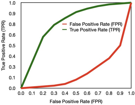
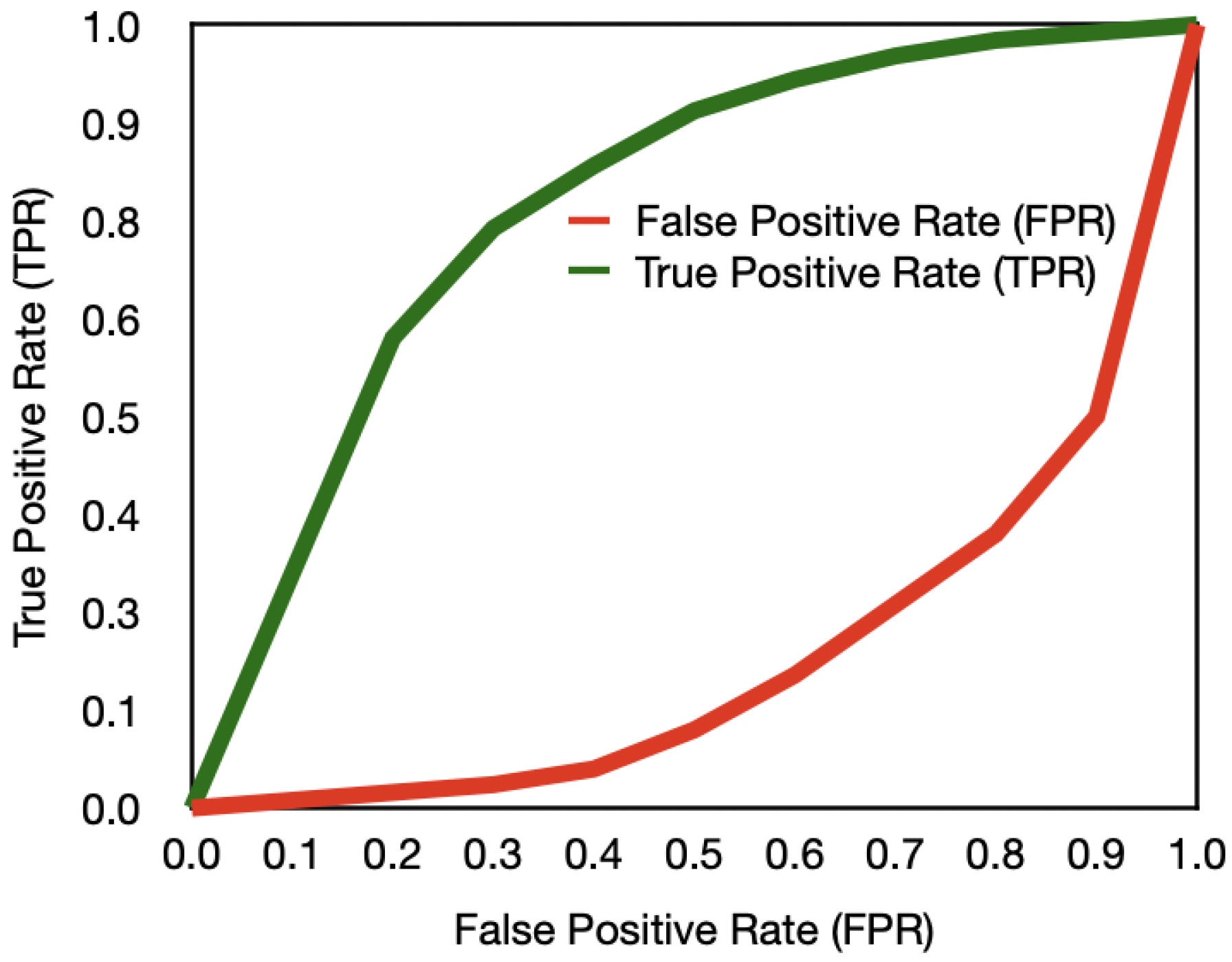
To further assess the classification capability of the LSTM model, we computed the Receiver Operating Characteristic (ROC) curve along with the Area Under the Curve (AUC) score. The ROC curve illustrates the trade-off between the True Positive Rate (TPR) and the False Positive Rate (FPR) across various decision thresholds. A model with perfect discrimination yields a curve that approaches the top-left corner of the plot, while a random classifier follows the diagonal.

As shown in Figure 4, the ROC curve of our model consistently outperforms the random baseline. The AUC score is 0.942, indicating excellent model performance and its strong ability to distinguish between failure and non-failure events in sequential sensor data.

Figure 4. ROC curve illustrating the trade-off between True Positive Rate (TPR) and False Positive Rate (FPR) for the trained LSTM model. The curve demonstrates strong classification performance, with an AUC score of 0.942.

Table 8 further highlights the impact of threshold variations on classification behavior. At the decision threshold of 0.5 used for the final reported metrics, the model achieves a TPR of 0.876 and an FPR of 0.076. The TPR at this operating point corresponds to a recall of 87.6%, consistent with the confusion matrix and the final classification metrics reported in this study.

Table 8. ROC Operating Points at Different Thresholds.

Threshold	True Positive Rate (TPR)	False Positive Rate (FPR)
0.3	0.960	0.220
0.5	0.876	0.076
0.6	0.890	0.060
0.7	0.850	0.040
0.9	0.720	0.010

6.6. Confusion Matrix Analysis

To better understand the classification behavior of the LSTM model, we analyzed the confusion matrix on the test dataset. Table 9 presents the distribution of predictions across four categories: True Positives (TP), True Negatives (TN), False Positives (FP), and False Negatives (FN).

Table 9. Confusion Matrix on Test Dataset.

	Predicted Failure	Predicted Normal
Actual Failure	588 (TP)	83 (FN)
Actual Normal	71 (FP)	858 (TN)

As shown in Table 9, the model correctly identified 588 failure instances and 858 normal cases. The confusion matrix is consistent with the reported accuracy, precision, recall, and F1-score in Table 4. These results indicate that the LSTM model maintains a balanced trade-off between detecting failure cases and limiting false alarms under the selected decision threshold.

6.7. Resource Usage Under Increasing Workload

To characterize the computational behaviour of the proposed predictive maintenance framework under increasing streaming workloads, we measured CPU usage, memory consumption, observed post-Spark prediction-stage latency, and processed prediction rate. The Kafka–Spark resource configuration was kept fixed across all evaluated workload levels. Therefore, the purpose of this analysis is to examine workload-dependent resource utilization and processing behaviour rather than empirical horizontal scalability.

Table 10 presents the system’s performance at three workload levels. At an input rate of 100,000 events per minute, the system used 28.5% of CPU and 540 MB of memory, with an observed post-Spark prediction-stage latency of 290 milliseconds and a processed prediction rate of 99.9%. As the event rate increased to 500,000 events/min, CPU usage increased to 42.3% and memory usage to 688 MB, while the processed prediction rate remained at 99.7% and the observed latency increased to 415 milliseconds.

Table 10. Resource Utilization Under Increasing Replay Workloads.

Event Rate	CPU Usage (%)	Memory (MB)	Latency (ms)	Processed Prediction Rate
100 K/min	28.5%	540	290	99.9%
500 K/min	42.3%	688	415	99.7%
1.2 M/min	63.7%	872	570	99.3%

Under the highest simulated workload of 1.2 million events per minute, CPU usage increased to 63.7%, memory usage reached 872 MB, and the processed prediction rate was 99.3%, with an observed post-Spark prediction-stage latency of 570 milliseconds. These results show that the fixed experimental configuration remained operational across the evaluated replay workloads, although resource consumption and observed latency increased with the incoming event rate. The results should therefore be interpreted as evidence of workload-dependent system behaviour under a fixed Kafka–Spark configuration rather than as an empirical demonstration of horizontal or linear scalability.

These resource-utilization results also provide an indication of the computational overhead of the proposed framework under the controlled replay conditions. The increases in CPU usage, memory consumption, and observed latency with higher streaming workloads indicate that computational cost is workload-dependent. Since LSTM training was performed offline, training time was not included in the reported prediction-stage latency. Furthermore, the reported latency does not represent complete Kafka–Spark–LSTM end-to-end latency, as Kafka queueing and Spark scheduling and processing times were not independently instrumented.

6.8. Component-Level Sensitivity Analysis

To examine the effect of key modelling and processing choices, we report a component-level sensitivity analysis under the simulated streaming setup. The purpose of this analysis is to show how changes in the predictive model and preprocessing pipeline affect classification performance and latency. The results are summarized in Table 11.

Table 11. Component-Level Sensitivity Analysis Under Simulated Streaming Conditions.

Configuration	Accuracy (%)	Latency (ms)	CPU Usage (%)
LSTM + Kafka/Spark + Normalization	90.4	415	42.3
Replace LSTM with GRU	89.1	408	41.5
Remove normalization layer	86.8	430	43.1
Direct batch processing without Kafka/Spark	90.4	570	26.8

The component-level sensitivity analysis shows that the LSTM-based configuration with normalization provides the strongest predictive performance among the tested model variants. Replacing the LSTM with a GRU slightly reduces classification performance, while removing normalization causes a more noticeable reduction in accuracy, indicating the importance of consistent feature scaling for multivariate sensor sequences. The direct batch-processing configuration achieves the same prediction accuracy of 90.4% because it uses the same trained LSTM model and the same preprocessed input features as the full Kafka–Spark–LSTM configuration. Kafka and Spark do not alter the learned predictive function of the LSTM and are therefore not intended to improve classification accuracy. Instead, Kafka provides buffered and scalable stream ingestion, while Spark Streaming supports continuous micro-batch processing of incoming data. Their contribution should therefore be interpreted primarily in terms of system-level streaming capability, including throughput, scalability, and pipeline responsiveness. The latency values in Table 11 are retained as descriptive observations under the respective simulated configurations. Because equivalent end-to-end timing boundaries were not instrumented across all pipeline components, these values are not used to quantify the independent latency contribution of Kafka or Spark.

7. Discussion

This section discusses the key strengths, practical relevance, and broader applicability of the proposed real-time predictive maintenance framework. We also reflect on its limitations and potential directions for future improvements.

7.1. Strengths and Real-World Applicability

The integration of Apache Kafka, Apache Spark Streaming, and LSTM models provides a replay-based architecture for evaluating predictive maintenance under simulated streaming conditions. The framework’s modular design makes it adaptable to IIoT-style data pipelines, while the CMAPSS dataset provides a controlled benchmark for studying aircraft engine degradation patterns. However, the results should be interpreted as simulation-based evidence rather than proof of deployment readiness in live industrial environments.

7.2. Handling Big Data Challenges

The proposed system explicitly addresses the three V’s of big data:

• Volume: Kafka’s distributed message queues and Spark’s processing mechanisms support high-volume replayed data streams. In the present fixed configuration, resource consumption and observed prediction-stage latency increased with workload, and the results should therefore be interpreted as workload-dependent behaviour rather than bottleneck-free scalability.
• Velocity: The Kafka–Spark architecture supports continuous stream processing, while the present experiments characterize prediction-stage timing under controlled replay conditions rather than complete sensor-to-alert latency.
• Variety: The framework supports heterogeneous sensor data formats (e.g., temperature, pressure, vibration), which are normalized and unified before prediction.

By leveraging scalable open-source technologies, the system demonstrates promising behaviour under controlled high-load replay conditions, but further validation using real streaming data and deployment logs is required before making strong claims about industrial robustness.

7.3. Potential for Adaptation and Continuous Learning

The current LSTM model is trained offline and does not implement incremental or online learning. The modular architecture could, in future work, be extended to support periodic retraining or model updates using newly collected sensor data. Such functionality would require additional implementation and experimental evaluation before claims regarding continuous learning or live model adaptation can be made.

7.4. Limitations of the Current Framework

Despite its strengths, the current system has certain limitations. First, the LSTM model is trained offline and does not incorporate incremental or online learning in its present form, which may reduce responsiveness to unseen fault types. Second, the framework assumes labeled training data, which may not always be available or correctly annotated in real-world industrial systems. Furthermore, while the CMAPSS dataset is a strong benchmark, real deployment scenarios may involve more noisy, sparse, or imbalanced data streams, which require advanced preprocessing or anomaly filtering.

The reported results are based on a single engine-level data split, with 15 independent engines in the held-out test set. Therefore, the aggregate metrics do not capture per-engine variability or uncertainty across alternative data splits. The results should consequently be interpreted within the evaluated experimental setting. Future work will consider repeated engine-level splits and per-engine uncertainty analysis to provide a more comprehensive assessment of generalization.

Furthermore, the streaming evaluation has two important limitations. First, the reported latency is measured from the availability of a processed Spark micro-batch to the generation of the corresponding prediction and therefore does not include Kafka ingestion/queueing or Spark micro-batch scheduling and processing time. Second, the original Spark micro-batch interval was not retained in the experimental logs, preventing exact replication of the streaming timing benchmark. In addition, system resources were held fixed while the replay workload was varied; consequently, the reported resource results characterize workload-dependent behaviour rather than empirical horizontal scalability. A fully instrumented end-to-end latency analysis and scaling study with varying Kafka partitions and Spark executors are left for future work.

7.5. Generalization to Other Domains

The framework may provide a basis for investigation in domains beyond aerospace, such as wind turbine monitoring, power grid fault detection, and smart manufacturing. However, applicability to these domains has not been evaluated in the present study. Transfer to a different domain would require domain-specific data, preprocessing, retraining, model and threshold configuration, and independent validation under the target operating conditions.

8. Conclusions and Future Work

This paper presented a replay-based big data framework for predictive maintenance in Industrial IoT environments, integrating Apache Kafka for data ingestion, Spark Streaming for stream processing, and an LSTM network for time-series fault prediction. Using the NASA CMAPSS FD001 dataset in a controlled replay-based setting, the LSTM model achieved 90.4% accuracy, while the observed post-Spark prediction-stage latency remained below 600 ms across the evaluated workload levels. Since the latency measurement begins after a processed Spark micro-batch becomes available for inference, the reported values should not be interpreted as complete Kafka–Spark–LSTM end-to-end latency. Similarly, because the Kafka–Spark resource configuration remained fixed while the incoming workload was varied, the resource-utilization results characterize workload-dependent system behaviour rather than empirical horizontal scalability. Overall, the results demonstrate the feasibility of integrating stream-processing technologies with deep learning for predictive maintenance evaluation under controlled replay conditions, while emphasizing the importance of clearly defined data-splitting, latency measurement, and reproducibility protocols.

Future work will focus on a fully instrumented evaluation of end-to-end pipeline latency, including Kafka ingestion and queueing, Spark scheduling and processing, and LSTM inference, together with explicit reporting of the micro-batch configuration. Horizontal scalability will also be evaluated by varying Kafka partitions, brokers, Spark executors, and computational resources under increasing workloads. In addition, future studies will investigate deployment of the predictive model on edge devices to reduce network dependency and support lower-latency fault detection closer to the data source. We also aim to incorporate explainable AI techniques to enhance the interpretability of model predictions for domain experts and explore federated learning for privacy-preserving collaborative model training across distributed industrial sites without sharing raw sensor data.

References

- Raja, G.B. Impact of IIOT in future industries: Opportunities and challenges. Internet Things 2021, 101–112. [Google Scholar]
- Peruthambi, V.; Pandiri, L.; Kaulwar, P.K.; Koppolu, H.K.R.; Adusupalli, B.; Pamisetty, A. Big Data-Driven Predictive Maintenance for Industrial IoT (IIoT) Systems. Metall. Mater. Eng. 2025, 31, 21–30. [Google Scholar] [CrossRef] [Scilit]
- Evans, M.R.; Oliver, D.; Zhou, X.; Shekhar, S. Spatial big data: Case studies on volume, velocity, and variety. In Big Data; CRC Press: Boca Raton, FL, USA, 2024; pp. 115–138. [Google Scholar]
- Malhotra, P.; Vig, L.; Shroff, G.; Agarwal, P. Long short term memory networks for anomaly detection in time series. In Proceedings of the 23rd European Symposium on Artificial Neural Networks (ESANN 2015), Bruges, Belgium, 22–24 April 2015; Volume 89, p. 94. [Google Scholar]
- Vollert, S.; Theissler, A. Challenges of machine learning-based RUL prognosis: A review on NASA’s C-MAPSS data set. In Proceedings of the 2021 26th IEEE International Conference on Emerging Technologies and Factory Automation (ETFA); IEEE: New York, NY, USA, 2021; pp. 1–8. [Google Scholar]
- Rojas, L.; Peña, Á.; Garcia, J. AI-driven predictive maintenance in mining: A systematic literature review on fault detection, digital twins, and intelligent asset management. Appl. Sci. 2025, 15, 3337. [Google Scholar] [CrossRef] [Scilit]
- Majumder, R.Q. Machine Learning for Predictive Analytics: Trends and Future Directions. Int. J. Innov. Sci. Res. Technol. 2025, 10, 3557–3564. [Google Scholar] [CrossRef] [Scilit]
- Bampoula, X.; Siaterlis, G.; Nikolakis, N.; Alexopoulos, K. A deep learning model for predictive maintenance in cyber-physical production systems using lstm autoencoders. Sensors 2021, 21, 972. [Google Scholar] [CrossRef] [Scilit]
- Yin, C.; Zhang, S.; Wang, J.; Xiong, N.N. Anomaly detection based on convolutional recurrent autoencoder for IoT time series. IEEE Trans. Syst. Man. Cybern. Syst. 2020, 52, 112–122. [Google Scholar] [CrossRef] [Scilit]
- Murarka, S.; Jain, A.; Singh, L. Advanced Techniques in Data Ingestion and Pipelining for Scalable Big Data Platforms: A Comprehensive Review. In Proceedings of the 2024 IEEE 4th International Conference on ICT in Business Industry & Government (ICTBIG); IEEE: New York, NY, USA, 2024; pp. 1–6. [Google Scholar]
- Zhang, N. A cloud-based platform for big data-driven cps modeling of robots. IEEE Access 2021, 9, 34667–34680. [Google Scholar] [CrossRef] [Scilit]
- Nagappan, K.; Subbiah, P.; Bellam, K.; Murugaiyan, M. Cloud, Fog, and Edge Computing for Industry 5.0. In Next Generation Data Science and Blockchain Technology for Industry 5.0: Concepts and Paradigms; IEEE: New York, NY, USA, 2025; pp. 149–186. [Google Scholar]
- Raptis, T.P.; Cicconetti, C.; Falelakis, M.; Kanellos, T.; Lobo, T.P. Design guidelines for Apache Kafka driven data management and distribution in smart cities. In Proceedings of the 2022 IEEE International Smart Cities Conference (ISC2); IEEE: New York, NY, USA, 2022; pp. 1–7. [Google Scholar]
- Shalaby, A.M.; Othman, N.S.; Shalaby, M. Impact of Dust and Sandstorms on 6G UAV Base Station Performance in Arid Saudi Arabian Environments. IEEE Access 2024, 12, 86194–86207. [Google Scholar] [CrossRef] [Scilit]
- Aleran, A.; Almukhalfi, H.; Noor, A.; Alluhaibi, R.; Hafez, A.; Noor, T.H. An IoT-based predictive maintenance framework using a hybrid deep learning model for smart industrial systems. Comput. Mater. Contin. 2026, 86, 93. [Google Scholar] [CrossRef] [Scilit]
- Khattach, O.; Moussaoui, O.; Hassine, M. End-to-end architecture for real-time IoT analytics and predictive maintenance using stream processing and ML pipelines. Sensors 2025, 25, 2945. [Google Scholar] [CrossRef] [Scilit]
- Tabbaa, H.; Ouedrhiri, O.; Kazaz, M.; Zaia, Y.; Baba, M.; Alichane, D.; Lachgar, M. Smart Factory: A real-time predictive maintenance platform based on microservices architecture and deep learning. SoftwareX 2026, 34, 102730. [Google Scholar] [CrossRef] [Scilit]
- Varalakshmi, K.; Kumar, J. Optimized predictive maintenance for streaming data in industrial IoT networks using deep reinforcement learning and ensemble techniques. Sci. Rep. 2025, 15, 27201. [Google Scholar] [CrossRef] [Scilit]
- Luu, H. Resilient Distributed Datasets. In Beginning Apache Spark 2: With Resilient Distributed Datasets, Spark SQL, Structured Streaming and Spark Machine Learning Library; Springer: Berlin/Heidelberg, Germany, 2018; pp. 51–86. [Google Scholar]
- Raptis, T.P.; Passarella, A. A survey on networked data streaming with apache kafka. IEEE Access 2023, 11, 85333–85350. [Google Scholar] [CrossRef] [Scilit]
- Joshi, P.K. Building High-Throughput Payment Transaction Systems with Kafka and Microservices. Int. J. Sci. Res. 2022, 11, 1658–1665. [Google Scholar] [CrossRef] [Scilit]
- Wang, Y.; Donta, P.K.; Lovén, L.; Dustdar, S.; Motlagh, N.H. Lightweight LSTM-Based Adaptive Kafka Tuning for Predictive IoT Data Streams. In Proceedings of the 2025 IEEE Fast Continuum Workshop, Helsinki, Finland, 7–12 July 2025. [Google Scholar]
- Koo, J.; Faseeh Qureshi, N.M.; Siddiqui, I.F.; Abbas, A.; Bashir, A.K. IoT-enabled directed acyclic graph in spark cluster. J. Cloud Comput. 2020, 9, 50. [Google Scholar] [CrossRef] [Scilit]
- Gruslys, A.; Munos, R.; Danihelka, I.; Lanctot, M.; Graves, A. Memory-efficient backpropagation through time. Adv. Neural Inf. Process. Syst. 2016, 29. [Google Scholar]
- Ong, K.S.H.; Niyato, D.; Friedrichs, T. Drift-Aware Edge Intelligence for Remaining Useful Life Prediction in Industrial Internet of Things. In Proceedings of the 2022 37th International Technical Conference on Circuits/Systems, Computers and Communications (ITC-CSCC); IEEE: New York, NY, USA, 2022; pp. 198–201. [Google Scholar]
- Krichen, M.; Mihoub, A. Long short-term memory networks: A comprehensive survey. AI 2025, 6, 215. [Google Scholar] [CrossRef] [Scilit]
- Ho, Y.; Wookey, S. The real-world-weight cross-entropy loss function: Modeling the costs of mislabeling. IEEE Access 2019, 8, 4806–4813. [Google Scholar] [CrossRef] [Scilit]
- Zhang, Z. Improved adam optimizer for deep neural networks. In Proceedings of the 2018 IEEE/ACM 26th International Symposium on Quality of Service (IWQoS); IEEE: New York, NY, USA, 2018; pp. 1–2. [Google Scholar]
- Wang, H.K.; Huang, H.Z.; Li, Y.F.; Yang, Y.J. Condition-based maintenance with scheduling threshold and maintenance threshold. IEEE Trans. Reliab. 2015, 65, 513–524. [Google Scholar] [CrossRef] [Scilit]
- Lakshmanaprabu, S.; Shankar, K.; Ilayaraja, M.; Nasir, A.W.; Vijayakumar, V.; Chilamkurti, N. Random forest for big data classification in the internet of things using optimal features. Int. J. Mach. Learn. Cybern. 2019, 10, 2609–2618. [Google Scholar] [CrossRef] [Scilit]
Disclaimer/Publisher’s Note: The statements, opinions and data contained in all publications are solely those of the individual author(s) and contributor(s) and not of MDPI and/or the editor(s). MDPI and/or the editor(s) disclaim responsibility for any injury to people or property resulting from any ideas, methods, instructions or products referred to in the content. |
© 2026 by the authors. Licensee MDPI, Basel, Switzerland. This article is an open access article distributed under the terms and conditions of the Creative Commons Attribution (CC BY) license.