


Abstract
Wind energy is becoming increasingly important in meeting energy security, grid reliability, and the growing electricity demand. The rapid increase in the number and prevalence of wind turbines has triggered the need for fast, cost-effective, reliable, and easy-to-implement inspection systems. Automated detection of coating defects is important for the maintenance and corrosion prevention of the turbines. In this context, this study aimed to compare and evaluate the accuracy and efficiency of deep learning models for detection of coating defects from images. In this context, the study evaluates five object detection models, RT-DETR-L, YOLOv8-M, YOLOv9-C, YOLO11-L, and YOLO26-L, on an open coating-defect dataset, with inclusion, pinhole, and scratch classes. Each model was trained with 3 random seeds for images of 640 × 640 and 1088 × 1088-pixel resolutions. At 1088 × 1088, YOLO26-L achieved the highest mean mAP50–95 (0.1142), while RT-DETR-L achieved the highest recall (0.5591) and F1 score (0.2217) at the operating confidence threshold of 0.25; RT-DETR-L was also the slowest model (59.8 ms/image). YOLOv8-M achieved a mean mAP50–95 of 0.0976 together with the lowest latency (34.2 ms/image) and lowest true batch-size-1 peak GPU-memory allocation (278 MB). Reducing the resolution to 640 × 640 lowered mAP50–95 by 25.4% for YOLOv8-M and 33.6% for RT-DETR-L while reducing latency and memory use. The results revealed a pronounced accuracy-efficiency trade-off rather than universal superiority of one model for coating defect detection for wind turbine towers. The dataset was acquired during the wind-tower painting process under controlled industrial imaging conditions, so the results characterise in-process coating inspection rather than the inspection of weathered, in-service turbines. Because only three random seeds were used, paired comparisons between individual models were not statistically conclusive (8 of 100 pairwise tests reached p < 0.05) and the reported rankings are descriptive. Applying operating thresholds—determined on the validation set for each model—to the independent test set altered the architectural ranking. At 1088 × 1088 resolution, YOLO26-L surpassed RT-DETR-L to achieve the highest mean F1 score, whereas at 640 × 640 resolution, RT-DETR-L’s ranking dropped significantly. The fact that the selected thresholds range from 0.076 to 0.456 indicates that the differences observed at the common threshold of 0.25 are sensitive to the choice of threshold. While the mAP50–95 decreased by approximately half in the 640 × 640 evaluation—where data leakage was eliminated—the 1088 × 1088 results were considered optimistic, as they were obtained based on the previous segmentation.
1. Introduction
The intensive consumption of fossil fuels such as coal, oil, and natural gas, which are the primary energy sources, leads to greenhouse gas emissions, global climate change, and environmental problems [1]. For these reasons, there has been a shift toward renewable energy sources. With increasing energy demand and environmental impacts, wind energy has gained increasing importance as a clean, sustainable and renewable energy source [2,3]. Wind is a horizontal movement of air caused by pressure differences in the atmosphere. Wind turbines convert the kinetic energy of the wind first into mechanical energy, and then into electrical energy via generators [4]. In 2025, the wind energy sector set a record with the installation of 165 GW of new capacity, representing a 40% increase compared to the previous year. Global wind energy capacity reached 1299 GW. 138 countries worldwide utilize wind energy, and in 2026, 28,395 wind turbines were installed in 57 countries. These findings demonstrate that wind energy is becoming increasingly important in meeting energy security, grid reliability, and growing electricity demand [5]. The position and importance of the wind energy industry have led to stricter requirements in operation and maintenance management regarding the reliability of wind energy equipment [6]. Figure 1 shows the change in primary energy use worldwide over the years.
Figure 1.
Changes in primary energy consumption worldwide by year [7,8].
Wind turbines generally consist of a tower, blades, rotor, gearbox, generator, and electrical and electronic components. Turbines are installed in areas where the wind blows unobstructed, and taller towers allow for the utilization of higher wind speeds [9].
Given the rapid increase in the number and prevalence of wind turbines, there is a need for a fast, cost-effective, reliable, and easy-to-implement inspection system. Traditional methods for defect detection in wind turbines generally rely on manual inspection. However, these methods are time-consuming, costly, and sensitive to environmental conditions [10]. This situation makes it difficult to safely and accurately detect minor defects in turbines exposed to high wind speeds [11].
Coatings used on large steel structures such as bridges and wind turbine towers are primarily in the protective coatings segment, aiming to protect structures from deterioration, decomposition, and especially corrosion. Selecting the appropriate coating system can increase the durability and service life of the structure while also providing functional properties [12]. High corrosion protection system reliability is essential in wind turbines. Coating systems for large steel structures are developed to provide high resistance to the environmental conditions to which they are exposed and to meet the necessary performance criteria; international standards such as ISO 12944 [13] and NORSOK [14] are used as a basis for the selection and evaluation of the performance of these systems.
In painting and coating processes, defects such as pits, holes, lack of filler, and scratches can result from equipment or environmental conditions [15,16]. Paint defects, particularly on wind turbine towers, can increase the risk of corrosion, negatively impacting equipment lifespan and reliability [17,18].
Early detection of coating defects enables timely planning of maintenance and repair, reducing corrosion progression and maintenance costs. Therefore, regular inspection of coatings is crucial for durability and sustainability. In recent years, computer vision and deep learning methods have yielded successful results in the automated detection of coating defects, accelerating inspection processes and reducing assessment errors. In this context, automated detection of wind turbine coating defects is an important research area in terms of structural health monitoring, quality control, and maintenance management.
This study aimed to compare and evaluate the accuracy and efficiency of deep learning models for the detection of coating defects from images. In this context, different object detection approaches based on deep learning were evaluated using the RT-DETR-L, YOLOv8-M, YOLOv9-C, YOLO11-L, and YOLO26-L models. Different versions of the models were developed on the open-source dataset available at [19]. In the experiments, the models were compared in terms of metrics such as mAP50, mAP50–95, Precision, Recall, and F1, and the most suitable model was determined. It is anticipated that the widespread adoption of these technologies will contribute to more effective planning of maintenance processes, reduction in operating and maintenance costs, and the safe, efficient, and sustainable operation of wind turbines.
The subsequent sections of this study are organized as follows: First, similar studies in the literature are reviewed within the scope of this research. In the Section 2, general methods used to detect damage in wind turbine towers are discussed and detailed information is provided on the object detection research field, the methodology applied in this study, and the YOLO and RTDETR algorithms used in this study. In the Section 3, a comparative analysis of the performance of the deep learning-based object detection models under examination is conducted. Finally, in the Section 4 and Section 5, the results are evaluated and discussed.
1.1. Literature Review
Table 1 gives a comparison of deep learning-based detection studies in wind turbines. Mao et al. (2021) [20] proposed an improved deep learning model called CAD Cascade R-CNN to classify and locate crack, fracture, and oil contamination defects in wind turbine blades. Experimental results showed that the proposed method exhibited high generalization ability across different defect types and IoU thresholds, and was more successful than Cascade R-CNN, Faster R-CNN, and YOLO-v3 models, with a mAP value of 92.1%. Zhang and Wen (2022) [21] proposed the YOLOv5-based SOD-YOLO model, which is based on UAV imagery. Experimental results showed that SOD-YOLO achieved 95.1% mAP, providing 7.82% higher accuracy and 28.3% higher FPS compared to YOLOv5. Zhang et al. (2023) [22] proposed a simplified YOLOv5s-based defect detection model for accurate and rapid detection of wind turbine surface defects. The average sensitivity increased by 5.51% compared to the original YOLOv5s model. Lu et al. (2023) proposed a novel approach combining principal component analysis (PCA) with the ResDenIncepNet-CBAM model to predict blade cracks using wind turbine SCADA data. Experimental results show that the proposed method is more successful than other classical convolutional neural network models, achieving an accuracy of 96.23%. To improve the economic efficiency of wind turbines, Ye et al. (2024) [23] proposed a YOLOv5s-based object detection model that identifies surface cracks in wind turbine blades from UAV imagery. Experimental results show that their proposed method is more successful than the original YOLOv5s in terms of both accuracy and speed. Altice et al. (2024) [24] used Xception, ResNet-50, AlexNet, VGG-19, and a custom CNN model, along with transfer learning approaches based on these architectures, to detect wind turbine blade damage. The results showed that the Transfer Xception model exhibited the most successful performance, achieving 99.92% accuracy in the test data. Li et al. (2024) [25] proposed an improved DeepLabv3+-based deep learning method for the detection and quantification of wind turbine blade surface defects. The results showed that the developed model reduced the training time by 43.03% and achieved an accuracy of 96.87% mAP and 96.93% mIoU. Davis et al. (2024) [26] compared YOLO and Mask R-CNN-based deep learning models for detecting defects such as cracks, holes, and wear on wind turbine blades. The results showed that the YOLOv9C model demonstrated the highest performance with 0.849 mAP50 and 0.539 mAP50–95. Mask R-CNN, developed with ResNet18-FPN, achieved a success rate of 0.8415 mAP50 while reducing computational complexity. Jiang et al. (2025) [27] proposed a lightweight small object detection model (LSOD-YOLO) based on YOLOv8 to detect wind turbine blade surface damage using drone imagery. Experimental results showed that LSOD-YOLO offers higher detection accuracy, smaller model size, and low-latency real-time performance compared to the basic YOLOv8 model. Lario et al. [28] evaluated the error detection performance of deep learning algorithms developed for Automated Visual Defect Detection for Wind Towers Painting Process using different datasets and training parameters. As a result, they obtained reliable results with YOLOv8 (mAP50 = 0.27, mAP50–95 = 0.12). Xiang et al. (2026) [29] proposed CoastCor-Net, based on YOLOv11, for Blade Defect Detection of onshore wind turbines. In experiments conducted on the Wind Turbine Blade Damage Dataset, CoastCor-Net achieved 84.7% mAP@0.5 and 54.1% mAP@0.5:0.95, outperforming YOLOv13n by 3.2 points in mAP@0.5 and 5.2 points in AP_damage. Feng et al. (2026) [30] proposed WB-YOLO, an improved YOLO model incorporating a P2 detection head and an Internal-SIoU loss function for detecting wind turbine surface defects. The proposed method achieved improvements of 1.9%, 2.5%, 2.1%, and 2.3% in Sensitivity, Recall, mAP@50, and mAP@50–95, respectively, compared to YOLO and DETR-based methods on the developed dataset, and reached an inference speed of 3.2 ms (312 FPS). Li et al. (2026) [31] proposed an improved YOLOv8n-based defect detection algorithm for accurate detection of small, fine defects on wind turbine blade surfaces under complex imaging conditions. Compared to YOLOv8n, the method increased the recall rate by 6.7% and the mAP@0.5 value by 2.2%. Wei et al. (2026) [32] proposed the YOLOv5-based CHBS-YOLO model to overcome the challenges in detecting wind turbine blade cracks. In the experimental results, CHBS-YOLO achieved 81.74% mAP on the wind turbine blade crack dataset, demonstrating 17.05%, 6.75%, 21.44%, and 1.47% higher performance than the EfficientDet, SSD, Faster R-CNN, and YOLOv5s models, respectively.
Table 1.
Comparison of deep learning-based detection studies in wind turbines.
1.2. Study Workflow
The experimental study compares five object-detection architectures for coating defects on wind-turbine tower surfaces, whereas most prior work focuses on wind-turbine blade defects or a single detector. The evaluation covers mAP50, mAP50–95, precision, recall, F1, variability across seeds, input resolution, inference latency, GPU memory, model size, and parameter count. Figure 2 summarizes the workflow. The workflow encompasses data preparation, training and evaluation, ablation studies, and cross-partition leakage checks. It also examines false alarms on flawless surfaces, operational thresholds determined through the validation process, and the impact of the Mosaic data augmentation method. The workflow comprises processes for data preparation, training and evaluation, ablation studies, and cross-partition leakage audit. It additionally examines false alarms on defect-free surfaces, operating thresholds determined through the validation process, and the effect of the Mosaic data augmentation method.
Figure 2.
Flowchart of the experimental methodology in this study.
In Phase 1, the open-source dataset was validated for image and annotation integrity and class balance. While 600 of the total 2697 images contained defects such as inclusions, pinholes, or scratches, the 2097 defect-free images were set aside for use in subsequent evaluations. The defective images were divided into training, validation, and test sets at a ratio of approximately 70%/10%/20% (421 training, 60 validation, and 119 test images), taking the defect classes into account. The same data partitioning process was applied at both 640 × 640 and 1088 × 1088 pixel resolutions. To preserve the aspect ratio while resizing the images, the relevant scaling and shifting operations were applied to the bounding boxes using the letterbox.
In Phase 2, the RT-DETR-L, YOLOv8-M, YOLOv9-C, YOLO11-L and YOLO26-L models were trained at both resolutions using a base Mosaic probability of 1.0 and random seed values of 0, 21, and 42. Using an early stopping method with a patience value of 20 epochs, the checkpoint yielding the highest validation mAP50–95 value was saved for each run. In addition to a fixed operating confidence threshold of 0.25, a specific threshold value was determined for each combination of model, resolution, and seed to maximize the validation F1 score; this value was then fixed prior to test evaluation. Without further retraining, the saved checkpoints were evaluated—without retraining—on both the test set consisting solely of 119 images containing defects and the background-enriched set (totaling 2216 images) created by combining these images with 2097 previously unseen defect-free images. The mAP value was calculated using a confidence threshold of 0.001. During the operating point evaluation, precision, recall, and F1 scores were compared under both the fixed threshold and the thresholds determined during the validation phase. The background evaluation also quantitatively analyzed false alarm behavior on defect-free surfaces. Results were compiled as means and standard deviations across seed values and supported by statistical comparisons. Latency, throughput, and peak GPU memory usage were measured under actual “batch size 1” inference conditions using the profiling process.
In Phase 3, resolutions of 640 × 640 and 1088 × 1088 pixels were compared in a resolution ablation study regarding accuracy, latency, and memory requirements. In a separate Mosaic ablation study, other hyperparameters were kept constant, and each setting was evaluated using three different random seeds. In this study, the YOLOv8-M model was tested at a resolution of 1088 × 1088 pixels with Mosaic probabilities of 1.0, 0.5, and 0.0. Finally, the existing dataset split was examined for inter-partition similarity using pixel hashes, perceptual hashes, and data collection timestamps. No changes were made to the dataset split as a result of this examination. Model rankings were interpreted descriptively, taking into account the limited number of random seeds used and the inter-partition similarity determined during the examination. Detailed analysis results are presented in Supplementary Tables S1–S16.
2. Materials and Methods
2.1. Dataset and Split
The source dataset [19] contained 2697 images and three defect classes: inclusion, pinhole, and scratch. The dataset used contains 2097 flawless background images (78%). The dataset of defect images consisted of 600 images. Defect-free images were excluded from the dataset as a result of a deliberate methodological choice aligned with the exploratory research objective of comparing the ability of different architectures to localize and distinguish subtle coating defects under controlled, defect-present conditions. Thus, the training set contained 421 images, and the validation set contained 60 images. The held-out test set used for evaluation contained 119 images.
Partitioning was stratified by the set of defect classes present in each image. Images are letterboxed to two square canvases: 1088 × 1088 and 640 × 640. Bounding boxes are transformed through the same scale + offset used for the image, so they stay pixel-accurate after padding. Representative examples from the dataset [19] are shown in Figure 3. This partitioning does not take acquisition sessions into account. As explained in 3.6, a second partitioning that considers data collection groups was subsequently created using the data collection metadata in the dataset, and all models were retrained using this new partitioning.
Figure 3.
Representative field images of the (a) inclusion, (b) pinhole, and (c) scratch classes in the dataset.
Excluding the 2097 defect-free images from the training process is a limitation of the training design. Since a detector that has never encountered defect-free coating surfaces cannot learn to reject them, the precision value measured on a test set consisting solely of defective images may appear higher than it actually is. Furthermore, the false positive rate on normal surfaces cannot be determined. To better illustrate this situation, all trained models were also evaluated on a separate set comprising a total of 2216 images formed by adding the 2097 defect-free images to the 119 defective test images, which was enriched with background variations. As none of these images were used during training, they all represent previously unseen negative samples for the models. The results of both evaluations are presented together in Section 3.3.
Various data augmentation techniques were used in the training process to make the model more robust against different image conditions and to reduce overfitting that may arise from the limited variety of training data. In this context, HSV color space changes, ±10% offset, ±50% scaling, horizontal flip with 50% probability, and mosaic augmentation with 1.0 probability were applied to the images. The aim was for the model to learn defects not only under specific color, position, and scale conditions, but also under different imaging conditions.
Following Ultralytics’ default training procedure, the Mosaic data augmentation method was applied with a probability of 1.0. However, to ensure each model converged on unaugmented images, this method was disabled for the final 10 epochs (close_mosaic = 10). Mosaic increases the effective sample diversity of a small dataset and multiplies the number of small objects observed per iteration. These characteristics are particularly significant given the availability of only 421 training images and 726 defect instances. Since continuous application of Mosaic could lead models to adapt to stitching artifacts rather than the appearance of the defects themselves, this choice was further evaluated through an ablation study presented in Section 3.5 based on the Mosaic probability.
2.2. Object Detection Models
Deep Learning is a subfield of Machine Learning that uses artificial neural networks and can process multidimensional data with multi-layered architectures. It is successfully used in many complex problems such as image processing, object detection and natural language processing (NLP) [33,34]. Object detection identifies the class of objects in an image and also determines their precise location in the image using bounding boxes. In this study, five object detection models, namely RT-DETR-L, YOLOv8-M, YOLOv9-C, YOLO11-L, and YOLO26-L, were evaluated in this study. Four of them utilized the YOLO architectures.
The models with a similar number of parameters were selected for evaluation to reduce comparison bias that might arise from model capacity. The models were kept within a range of approximately 24–32 million parameters. In this context, the YOLOv8 model was used in its Medium (M) version rather than the Large (L) version to align its model size with that of the other detectors. Therefore, in selecting the other YOLO models, the goal was to ensure a comparison that was as balanced as possible by basing the selection on models with capacities close to that of RT-DETR-L. Table 2 provides information about the architectures of the object detection models used in the study.
Table 2.
Object detection models compared in the study.
2.2.1. Real-Time Detection Transformer (RT-DETR)
Detection Transformer (DETR) is an object detection algorithm developed by the Facebook AI team in 2020 and based on the Transformer architecture [40]. Real-Time Detection Transformer (RT-DETR) was developed to increase the speed and efficiency of DETR models, which offer high accuracy but are limited in real-time applications. RT-DETR [35] made real-time object detection possible by redesigning the transformer architecture. The model simplifies the detection process by simultaneously performing classification and bounding-box regression [41]. Comprising a CNN-based feature extractor, a lightweight Transformer encoder–decoder architecture, and multi-head attention mechanisms, RT-DETR offers a balanced performance between accuracy and speed for real-time applications [35]. Figure 4 shows the RT-DETR architecture.
Figure 4.
RT-DETR architecture. (Adopted from [35]).
2.2.2. You Only Look Once (YOLO)
You Only Look Once (YOLO) is a fast and efficient object detection method used in image processing. Unlike traditional methods, it analyzes the entire image at once, simultaneously estimating the classes and bounding boxes of objects. This combined approach enables YOLO to offer high speed and accuracy in real-time applications. Since its first version was developed in 2016 by Redmon et al. [42], the YOLO family has been continuously improved and different versions have been produced with increased accuracy, speed, and computational efficiency. The YOLO architecture consists of three main components (backbone, neck, and head) that perform feature extraction and object detection from the image. The backbone extracts basic visual features at different scales from the input image through Convolutional Neural Network (CNN)-based structures. The neck combines the features obtained from the backbone, particularly strengthening spatial and semantic information at different scales. The head generates the final prediction results [43,44].
The YOLO architecture has been continuously optimized to improve the balance between accuracy and speed [45]. By improving the backbone, neck, and head components, the sensing process has been simplified, and data loss and computational load have been reduced (Figure 5). The models used in the study were YOLOv8, YOLOv9, YOLO11, and YOLO26. Of these models, YOLO26 is one of the recent examples of this development process.
Figure 5.
Evolution of YOLO architectures [46,47].
2.3. Training and Evaluation Setup
Training and evaluation were performed with Python 3.13.14, PyTorch 2.10.0 (CUDA build cu130) [48], CUDA 13.0 [49], and Ultralytics 8.4.18 [50] on an NVIDIA GeForce RTX 4060 Ti GPU with 16 GB memory. All models were initialized from their respective official COCO-pretrained checkpoints (Ultralytics release weights) and fine-tuned on the coatings-defect dataset for up to 100 epochs using the AdamW optimizer (initial learning rate 0.001, cosine schedule with Final LR ratio of 0.01, weight decay 5 × 10⁻⁴, number of warm-up epochs 3. The physical batch size was 8, with gradient accumulation to an effective batch size of 16; automatic mixed precision and deterministic mode were enabled. Fixed seed values (0, 21, 42) were used during training.
In this study, instead of relying on a single random run, each model is trained with three independent runs with seed = 0, seed = 21, and seed = 42 to evaluate variance in model performance. Models were trained for a maximum of 100 epochs. However, to reduce unnecessary training time, prevent overtraining, and terminate training when validation performance no longer improves, an early termination with 20 epochs of patience was implemented. Detection performance was evaluated using two confidence thresholds, each chosen for a specific purpose. A confidence threshold of 0.001 was used to calculate mAP50 and mAP50–95 across the precision–recall curve. Precision, recall, and F1 were reported at the fixed operating confidence threshold of 0.25, which was also used for deployment-oriented detection counts and latency measurements. Both confidence thresholds and the IoU threshold of 0.5 were defined before evaluation and were not adjusted based on the test results. For each model, the checkpoint with the best validation performance (mAP50–95) during training was used for the final evaluation.
2.4. Performance Evaluation Metrics
Object-detection performance was evaluated using true positives (TP), false positives (FP), and false negatives (FN) after confidence and IoU matching. Unlike ordinary image classification, true negatives are not generally enumerated over all possible background boxes and were not used in the reported detection metrics.
The reported metrics are mAP50, mAP50–95, precision, recall, and F1 score. Precision is TP/(TP + FP), recall is TP/(TP + FN), and F1 is the harmonic mean of precision and recall. AP is the area under the precision–recall curve for a class. mAP50 averages AP across classes at IoU = 0.50, whereas mAP50–95 averages AP across classes and IoU thresholds from 0.50 to 0.95 in steps of 0.05 (Table 3).
Table 3.
Performance metrics.
The prediction time of the models was also measured. The aim was to reliably measure how long each model took to process a single image. Latency measurement was performed using a batch size of 1, 10 warm-up iterations, followed by up to 200 timed iterations. This was taken into consideration, especially in terms of future real-time applications.
3. Results
3.1. Detection Accuracy and Computational Efficiency
This section reports validation- and held-out test-set performance for five object detectors trained with the same configured optimization settings and three random seeds (0, 21, and 42). Table 4 presents the validation set performance of the models.
Table 4.
Summary statistics of the validation-set performance metrics across random seeds.
The results show that model rankings varied according to both resolution and evaluation metric. At 640 × 640, YOLOv9-C achieved the highest mean mAP50 (0.3033), mAP50–95 (0.1092), and F1 score at a confidence threshold of 0.25 (0.1938). YOLO26-L produced the highest precision (0.7976), but its low recall (0.0811) indicates that this high precision was achieved by retaining relatively few detections. RT-DETR-L achieved the highest recall (0.4791), although its low precision (0.1489) limited its F1 score to 0.1871. YOLOv8-M showed a comparatively balanced performance, with an mAP50–95 of 0.0908 and an F1 score of 0.1749.
At 1088 × 1088, YOLO11-L achieved the highest mAP50 (0.3628) and mAP50–95 (0.1430), with relatively low variation in mAP50–95 across seeds (±0.0130). YOLOv9-C produced the highest precision (0.8022), but its recall remained low (0.0983). RT-DETR-L again achieved the highest recall (0.4539), whereas YOLOv8-M obtained the highest F1 score (0.2296), indicating the most favorable balance between precision and recall at the selected confidence threshold.
The effect of increasing the input resolution was architecture-dependent. YOLO11-L, YOLO26-L, and YOLOv8-M showed clear improvements in both mAP50 and mAP50–95 at 1088 × 1088. RT-DETR-L exhibited an increase in mAP50–95 from 0.0725 to 0.1005, despite a reduction in mAP50 from 0.2833 to 0.2236. In contrast, YOLOv9-C performed better at 640 × 640 for both mAP measures, with mAP50–95 decreasing from 0.1092 to 0.0767 at the higher resolution.
The standard deviations indicate that performance stability also differed among models and metrics. The relatively low variability of YOLO11-L at 1088 × 1088 suggests consistent validation accuracy across seeds. In contrast, several precision, recall, and F1 estimates particularly for YOLO11-L, YOLO26-L, YOLOv8-M, and YOLOv9-C at 1088 × 1088 showed substantial seed-to-seed variation. Because only three seeds were evaluated, small differences should be interpreted cautiously. Overall, higher resolution benefited most architectures, but the size and consistency of the improvement depended on the detector and the metric considered.
Table 5 summarizes the test-set performance of the five object-detection models at input resolutions of 640 × 640 and 1088 × 1088 pixels.
Table 5.
Summary statistics of the test-set performance metrics across random seeds.
At 1088 × 1088, YOLO26-L achieved the highest mean mAP50 (0.3112) and mAP50–95 (0.1142). YOLOv9-C produced the highest precision at the fixed confidence threshold of 0.25 (0.8262), although its comparatively low recall (0.0913) indicates a conservative detection profile in which relatively few predictions were retained. RT-DETR-L achieved the highest recall (0.5591) and F1 score (0.2217), reflecting a more balanced precision–recall trade-off. YOLO11-L and YOLOv8-M showed intermediate performance, while YOLOv9-C recorded the lowest mAP50 (0.2190) and mAP50–95 (0.0713) at this resolution.
At 640 × 640, the relative ranking varied across metrics. YOLOv9-C achieved the highest mAP50 (0.2417), while YOLO26-L retained the highest mAP50–95 (0.0839) and produced the highest precision (0.7818). RT-DETR-L achieved the highest recall (0.5105) and F1 score (0.1800). Although YOLO26-L showed high precision, its low recall (0.0764) resulted in a relatively modest F1 score (0.1113), suggesting that many ground-truth defects were not detected at the selected confidence threshold.
Increasing the input resolution improved both mAP50 and mAP50–95 for RT-DETR-L, YOLO11-L, YOLO26-L, and YOLOv8-M. The largest absolute improvement in mAP50–95 was observed for RT-DETR-L, increasing from 0.0695 to 0.1046. YOLOv9-C was the only model for which both mAP measures decreased at the higher resolution, with mAP50 declining from 0.2417 to 0.2190 and mAP50–95 from 0.0796 to 0.0713. Precision generally increased at the higher resolution, except for YOLO26-L, whereas recall and F1 improved for all models except YOLOv9-C. These findings demonstrate that the effect of input resolution depends on both the architecture and the performance metric considered.
Several model–metric combinations exhibited relatively large standard deviations across the three random seeds. This was particularly evident for the mAP values of YOLO26-L at 1088 × 1088 and for some precision, recall, and F1 estimates. Consequently, small differences between models should be interpreted cautiously, particularly given the limited number of training seeds. Overall, higher resolution generally improved detection performance, but the magnitude and consistency of the improvement remained architecture-dependent.
In Figure 6, each curve illustrates the trade-off between precision and recall as the confidence threshold varies, while the filled marker indicates the operating point obtained using the fixed deployment confidence threshold of 0.25. Curves located closer to the upper-right region represent a more favorable balance between detecting a greater proportion of defects and limiting false-positive predictions.
Figure 6.
Precision-Recall Curves for 1088 × 1088 resolution test set.
RT-DETR-L maintains comparatively high precision over a broad recall range and reaches the highest recall at the selected operating point (0.5591). However, its operating-point precision is relatively low (0.1500), indicating that the increased detection coverage is accompanied by more false-positive predictions. YOLO26-L displays a favorable overall precision–recall profile and achieves the highest mAP50–95 among the evaluated models. At the confidence threshold of 0.25, it provides substantially higher precision (0.7059) but lower recall (0.1686) than RT-DETR-L.
YOLO11-L and YOLOv8-M occupy an intermediate region of the plot. Their operating points show similar recall values of 0.1426 and 0.1739, respectively, with precision values of 0.5975 for YOLO11-L and 0.6736 for YOLOv8-M. YOLOv9-C achieves the highest operating-point precision (0.8262), but its recall is the lowest (0.0913). This indicates a conservative detection pattern in which most retained predictions are correct, although a considerable proportion of ground-truth defects remain undetected.
Overall, the figure demonstrates that model selection depends on the intended inspection objective. RT-DETR-L may be preferable when detecting as many potential defects as possible is the main priority, whereas YOLOv9-C provides fewer but more reliable detections at the selected confidence threshold. YOLO26-L offers the strongest overall accuracy according to mAP50–95 and provides a more balanced compromise between these two operating characteristics. The distinct locations of the confidence-threshold markers also show that performance comparisons based on a single operating point should be interpreted together with the complete precision–recall curves.
Table 6 presents the number of ground-truth bounding-box instances for each defect class across the training, validation, and test sets. The dataset shows substantial class imbalance at the instance level. Of the 726 annotated defects, 560 are inclusions (77.1%), 138 are pinholes (19.0%), and only 28 are scratches (3.9%). This imbalance is particularly pronounced in the validation and test sets, which are used for model selection and final performance reporting. The validation set contains only two scratch instances out of 78 total annotations, while the test set contains five out of 153.
Table 6.
Class-instance counts (bounding boxes).
Since the test set contains only five scratch samples, the recall value for this class can take only six different values and varies in 0.20 increments. A single additional correct or incorrect detection can change the scratch AP50 value by up to 0.200. This amount exceeds the total range of scratch AP50 values observed across all five architectures (range: 0.032–0.105). Consequently, the results for the scratch class are presented solely for the sake of completeness. These results are not statistically distinguishable, and no claim is made regarding any ranking among the architectures within this class. The same caution applies, less severely, to the pinhole class.
Figure 7 presents class-specific AP50 performance at 1088 × 1088 resolution, averaged across three random seeds. AP50 measures detection accuracy for each defect class using an intersection-over-union threshold of 0.50.
Figure 7.
AP50 by defect class-1088 × 1088.
YOLOv8-M achieved the highest AP50 for inclusions (0.457), closely followed by RT-DETR-L (0.448) and YOLO11-L (0.440). In contrast, YOLO26-L provided the strongest performance for pinholes (0.494) and scratches (0.105). RT-DETR-L achieved the second-highest pinhole AP50 (0.386), whereas its scratch AP50 remained low (0.061).
Across all architectures, scratches were substantially more difficult to detect than inclusions and pinholes, with AP50 values ranging from 0.038 to 0.105. This consistently weak performance may reflect the elongated, thin, and low-contrast appearance of scratches, as well as their limited representation in the dataset. However, because only a small number of scratch instances were available for training and testing, the class-level results are subject to considerable uncertainty and should not be interpreted as definitive evidence of an architectural limitation. Overall, no single model achieved the best performance across all defect classes: YOLOv8-M was most effective for inclusions, whereas YOLO26-L showed greater sensitivity to pinholes and scratches. These findings emphasize the importance of reporting class-specific performance alongside aggregate detection metrics when selecting a model for practical coating-defect inspection.
Figure 8 shows the relationship between the mAP50–95 values of the models and their mean inference latencies. Hollow and filled circles represent the 640 × 640 and 1088 × 1088 configurations, respectively. Circle size indicates peak GPU-memory consumption, and the dotted lines connect the two resolutions of each model.
Figure 8.
mAP50–95 vs. Mean Latency (Filled circle = 1088 × 1088. Hollow circle = 640 × 640; circle area is proportional to peak GPU memory under true batch-size-1 inference, and dotted lines connect the two resolutions of the same model).
Increasing the input resolution consistently increased inference latency and GPU-memory consumption. However, the corresponding change in accuracy was architecture-dependent. YOLO26-L achieved the highest mAP50–95 at 1088 × 1088, although this gain was accompanied by increased latency and memory demand. RT-DETR-L also showed a substantial improvement at the higher resolution but remained the slowest architecture. YOLO11-L achieved a favorable improvement in accuracy with a more moderate latency increase, while YOLOv8-M provided the lowest latency at both resolutions and retained competitive detection performance. In contrast, YOLOv9-C showed a reduction in mAP50–95 when the input resolution was increased, despite requiring more inference time and GPU memory.
Overall, the figure demonstrates that higher spatial resolution does not provide a uniform benefit across detection architectures. YOLO26-L favors accuracy, YOLOv8-M favors computational efficiency, and YOLO11-L offers a comparatively balanced accuracy–latency profile. RT-DETR-L may be appropriate when accuracy is prioritized over inference speed, whereas the higher-resolution YOLOv9-C configuration appears less favorable because it increases computational cost without improving accuracy. These findings emphasize that model selection should consider accuracy, latency, and memory requirements jointly rather than relying on a single performance metric.
Table 7 compares the accuracy and computational requirements of the five evaluated models at input resolutions of 1088 × 1088 and 640 × 640 pixels. The reported indicators include mAP50–95, inference latency, throughput, peak GPU memory consumption under true batch size = 1 inference, and parameter count.
Table 7.
Comparison of model performance and computational metrics.
Peak GPU memory usage was measured during single-image inference (batch size = 1) to represent a realistic deployment setting. For each trained model, the corresponding checkpoint was loaded onto the GPU, followed by ten warm-up inference runs. This warm-up step prevented one-time processes, including CUDA context initialization and kernel-cache construction, from affecting the measurements. The model was then run separately on each of the 119 images in the held-out test set, with GPU operations explicitly synchronized before and after every inference call. The highest memory allocation observed during the complete test-set run was reported as the model’s peak inference memory footprint.
At 1088 × 1088, YOLO26-L achieved the highest mAP50–95 (0.1142), followed by RT-DETR-L (0.1046), YOLOv8-M (0.0976), and YOLO11-L (0.0940). YOLOv9-C produced the lowest accuracy at this resolution (0.0713). However, the greater accuracy of YOLO26-L and RT-DETR-L was accompanied by higher computational demand. RT-DETR-L was the slowest model, requiring 59.8 ms per image and processing 16.7 images/s. It also had the highest peak GPU memory consumption (408 MB) and the largest parameter count (31.99 million).
YOLOv8-M provided the strongest computational efficiency at 1088 × 1088. It achieved the lowest latency (34.2 ms), highest throughput (29.2 images/s), and lowest peak GPU-memory consumption (278 MB), while maintaining a competitive mAP50–95 of 0.0976. YOLO26-L offered a balanced accuracy–efficiency profile, attaining the highest accuracy with a latency of 42.3 ms and a peak memory requirement of 394 MB. YOLO11-L showed similar computational requirements but slightly lower accuracy. YOLOv9-C was less favorable at this resolution because it combined the lowest mAP50–95 with comparatively high latency and memory use.
Reducing the resolution to 640 × 640 improved inference speed and reduced memory consumption for every architecture. YOLOv8-M remained the fastest and most memory-efficient model, achieving 18.1 ms per image, 55.3 images/s, and a peak memory requirement of 161 MB. YOLO26-L retained the highest mAP50–95 at the lower resolution (0.0839), followed by YOLOv9-C (0.0796). YOLOv9-C was the only architecture whose mAP50–95 increased when the resolution was reduced, indicating that the benefit of higher spatial resolution was architecture-dependent.
Overall, the results demonstrate a clear trade-off between detection accuracy and computational efficiency. YOLO26-L is the preferred option when accuracy is the primary objective, whereas YOLOv8-M is better suited to latency- and memory-constrained environments. RT-DETR-L provides competitive accuracy but incurs the greatest computational cost. Parameter count alone does not fully explain these differences, as the similarly sized YOLO models exhibit distinct latency and memory profiles.
3.2. Resolution Ablation
Figure 9 provides a comparison of detection performance to help in understanding the impact of image resolution on detection performance of the models.
Figure 9.
Resolution Comparison of test-set detection performance.
Increasing the resolution improved both mAP50 and mAP50–95 for four of the five models, although the magnitude of improvement varied considerably across architectures. RT-DETR-L exhibited the largest relative gain: its mAP50 increased from 0.1948 to 0.2981, while its mAP50–95 rose from 0.0695 to 0.1046, corresponding to improvements of approximately 53.0% and 50.5%, respectively. YOLO26-L achieved the highest overall performance at 1088 × 1088, with an mAP50 of 0.3112 and an mAP50–95 of 0.1142, compared with 0.2389 and 0.0839 at 640 × 640.
YOLOv8-M also benefited substantially from the higher resolution, with mAP50 increasing from 0.2230 to 0.2946 and mAP50–95 from 0.0728 to 0.0976. Similarly, YOLO11-L improved from 0.2234 to 0.2726 in mAP50 and from 0.0684 to 0.0940 in mAP50–95. These gains suggest that the additional spatial information available at 1088 × 1088 improves the representation and localization of small or visually subtle coating defects.
YOLOv9-C was the only architecture that did not benefit from the increased resolution. Its mAP50 decreased from 0.2417 at 640 × 640 to 0.2190 at 1088 × 1088, while its mAP50–95 declined from 0.0796 to 0.0713. This result indicates that a larger input size does not necessarily improve detection performance and may introduce architecture-specific optimization or feature-representation challenges.
Overall, 1088 × 1088 was the more effective resolution for RT-DETR-L, YOLO11-L, YOLO26-L, and YOLOv8-M, whereas 640 × 640 was more favorable for YOLOv9-C. The findings therefore demonstrate that the effect of input resolution is architecture-dependent rather than universally beneficial. Because the results represent means across only three random seeds and several model configurations exhibited substantial between-seed variation, the observed differences should be interpreted as comparative trends rather than statistically definitive rankings.
3.3. Background-Augmented Evaluation
Table 8 compares operating-point performance on the two held-out sets: the defect-only set of 119 images used above, and the background-augmented set of 2216 images that adds all 2097 defect-free images. The checkpoints, defect images and annotations are identical in both; the only change is the presence of unseen defect-free coating.
Table 8.
Precision on the defect-only and background-augmented held-out test sets at 1088 × 1088, conf = 0.25 (mean ± sd over seeds 0/21/42). Per-seed values are given in Supplementary Table S9.
Precision decreased for every architecture once defect-free surfaces were present, by 13.8% (YOLOv9-C) to 69.6% (RT-DETR-L) in relative terms at 1088 × 1088. Recall was essentially unchanged, as expected, because the defect images and their descriptions are identical in both sets. The entire observed effect consists of additional false-positive detections appearing on defect-free coating.
Table 9 quantifies this effect. At a working threshold of 0.25, RT-DETR-L detected at least one defect in 845 of 2097 defect-free images (40.3 ± 10.8%). In total, it generated 2340 ± 1124 false positives (1.12 ± 0.54 per defect-free image). Convolutional detectors, on the other hand, exhibited a significantly more conservative approach, with false positive rates of 3.5% (YOLOv9-C), 5.1% (YOLO11-L), 6.0% (YOLO26-L), and 6.5% (YOLOv8-M), with fewer than 0.09 false boxes per image. This ranking remained valid at a resolution of 640 × 640 as well. While RT-DETR-L reached a rate of 37.9%, convolutional models remained within the range of 3.5% to 10.1%. Unlike the accuracy rankings discussed in Section 3.4, this difference is statistically significant. RT-DETR-L differs from all other architectures at the p < 0.05 level (Welch’s t-test, p = 0.017–0.021), and the random seed ranges do not overlap. The best RT-DETR-L seed (27.8%) outperformed even the worst convolutional model seed (10.1%). Since there were only three random seeds per model, these rates were reported only descriptively, and no claims of statistical significance were made based on the averages. To compare the architectures more reliably, the predictions obtained from 2097 defect-free images were matched on an image-by-image basis and compared using the exact McNemar test. Thus, the unit of analysis became 2097 images instead of three seeds. At 640 × 640 resolution, RT-DETR-L was found to be significantly different from all convolutional detectors in this matched analysis (n = 2097; exact McNemar test; all p < 0.001 after Holm correction for 10 model pairs). Per-seed values are given in Supplementary Table S10, and the paired per-image McNemar analysis that supersedes the earlier seed-level significance tests is in Supplementary Table S19.
Table 9.
False alarms on the 2097 defect-free coating images at conf = 0.25, 1088 × 1088 (mean ± sd over seeds 0/21/42).
These results qualify the recall advantage reported for RT-DETR-L in Table 5. Its higher sensitivity on defect-containing images is obtained together with a detection tendency on defect-free surfaces roughly seven times that of the convolutional detectors. In an inspection setting where the large majority of acquired images are defect-free, this trade-off is unfavourable, and model selection should therefore weigh false-alarm behaviour on clean surfaces alongside defect-side recall.
3.4. Operating-Threshold Selection
The results above were obtained at a single confidence threshold of 0.25 applied to every architecture. To test whether that common threshold favours some detectors over others, an operating threshold was selected independently for each model, resolution and seed by maximising F1 on the validation split alone, and was then frozen and applied unchanged to the held-out test set. The test set was not consulted at any point during selection. Table 10 reports the outcome. Per-seed values for both test sets and both resolutions are given in Supplementary Table S11.
Table 10.
Operating thresholds τ* selected on the validation split alone and then frozen and applied unchanged to the held-out test set, 1088 × 1088 (mean ± sd over seeds 0/21/42). The τ = 0.25 column is the fixed threshold.
The selected thresholds differ substantially between architectures, ranging from 0.076 ± 0.018 for YOLOv9-C to 0.456 ± 0.171 for RT-DETR-L at 1088 × 1088, a factor of six. The common value of 0.25 therefore lies well above the optimum for some detectors and well below it for others. Using each model’s own threshold improved F1 for every architecture at 1088 × 1088 by between 17% (RT-DETR-L) and 60% (YOLOv9-C).
The ranking is also affected. At 1088 × 1088, the highest mean F1 shifts from RT-DETR-L to YOLO26-L. At 640 × 640, the reordering is more pronounced: under the fixed threshold, the ordering is RT-DETR-L > YOLOv9-C > YOLOv8-M > YOLO26-L > YO-LO11-L, whereas under per-model thresholds it becomes YOLO11-L > YOLOv8-M > YOLOv9-C > YOLO26-L > RT-DETR-L, moving RT-DETR-L from first to last. Part of the advantage attributed to RT-DETR-L at the lower resolution is thus an artefact of the shared threshold rather than a property of the architecture. Comparisons at a single fixed confidence value should accordingly be interpreted with caution, and per-model calibration is recommended before any deployment decision. In Table 11, RT-DETR-L moves from first to last.
Table 11.
Model ranking by F1 at 640 × 640 under the fixed threshold τ = 0.25 and under per-model validation-selected thresholds τ*.
3.5. Mosaic Augmentation Ablation
In the analyses, following Ultralytics’ default method, the Mosaic augmentation was applied with a probability of 1.0, and this setting was tested. While keeping all other hyperparameters constant, the YOLOv8-M model was retrained using the same three random seeds with Mosaic probabilities of 0.5 and 0.0 (Table 12). Per-seed values and the significance tests are given in Supplementary Table S14.
Table 12.
Mosaic-probability ablation for YOLOv8-M at 1088 × 1088, three seeds per arm, with every other hyperparameter held fixed.
The results are presented in Table 12. The mosaic = 1.0 setting yielded the best performance, with a mean mAP50–95 value of 0.0976 ± 0.0181, compared to 0.0871 ± 0.0433 for mosaic = 0.5 and 0.0802 ± 0.0185 for mosaic = 0.0. The same ranking held true for mAP50 and the F1 score at the operating threshold. None of these differences were statistically significant across three different random seeds (Welch’s t-test; p = 0.73 and p = 0.31); in fact, the spread of values within the mosaic = 0.5 group alone (0.044 to 0.131) exceeded the difference between the groups. Thus, the findings indicate that applying the mosaic data augmentation method with a probability of 1.0 did not reduce accuracy on this dataset.
3.6. Acquisition-Group-Aware Re-Evaluation
The evaluation reported above was based on a segmentation in which defect-only images are stratified solely according to class distribution. Since this approach does not take shooting sessions into account, similar images captured seconds apart during the same session may have been assigned to both the training and test sets. During the review, 33 identical, 489 nearly identical, and 216 cross-split image pairs with a time difference of less than 60 s between captures were identified. It was observed that one training-test pair was captured just 1 s apart.
To prevent this potential data leakage, the dataset was re-split to ensure that images from the same acquisition session remained within the same partition. The 600 defective images were organized into 10 acquisition groups. These groups were verified using timestamps from the source filenames, confirming that image similarity decreased as the time difference increased. By evaluating all group assignments and balancing a split ratio of approximately 70/10/20 with the requirement that every class is represented in each partition, a new split was established comprising 437 training, 53 validation, and 110 test images.
In the new split, the number of identical cross-split image pairs dropped from 33 to 0, and nearly identical pairs fell from 489 to 26; furthermore, cross-split pairs with time intervals of less than 60 or 600 s were completely eliminated. The remaining 26 similar pairs consist of visually similar surface images captured on different days under varying imaging conditions, and thus could not be separated through session-based grouping.
Previous models were not simply re-evaluated on the new test set; instead, they were retrained while maintaining the same hyperparameters and COCO pre-trained initial weights. Thus, the key variable between the two evaluations was data partitioning.
The results are presented in Table 13. Keeping images from the same acquisition session within the same split led to a 34–80% drop in mAP50–95 values, depending on the architecture, with an average decline of 49.8%. The model ranking based on F1 thresholds shifted from YOLO11-L > YOLOv8-M > YOLOv9-C > YOLO26-L > RT-DETR-L to YOLO26-L > YOLO11-L > YOLOv8-M > YOLOv9-C > RT-DETR-L. However, since only three seeds were used, this ranking should be considered descriptive. The largest drop was observed for RT-DETR-L (79.6%), a result consistent with the tendency for false alarms on defect-free surfaces reported in Section 3.3. Overall, the findings indicate that absolute accuracy values obtained via class-stratified splitting can decrease significantly when evaluated in a manner that is distinct regarding data acquisition.
Table 13.
Accuracy on the class-stratified split (as previously reported) and on the acquisition-disjoint split, 640 × 640, mean +/− sd over seeds 0/21/42.
It should be noted that the test set, separated based on data acquisition, was not created merely by removing similar pairs from the previous test images. Due to the preservation of group integrity, the test set contains 110 images instead of 119, and the class distribution also differs. Consequently, the observed performance difference reflects the impact of a different test distribution in addition to the elimination of data leakage.
The re-evaluation was conducted at a resolution of 640 × 640 using five architectures and three seeds. However, the results at 1088 × 1088 resolution were obtained using the existing class-stratified split. Since the same image partitioning is used for both resolutions, the 1088 × 1088 results are also affected by the same data leakage channel. Therefore, the re-evaluation of discrete partitioning regarding data collection was limited to the 640 × 640 resolution, and the obtained results were interpreted within the context of the impact of partitioning variations on model performance. Evaluating the 1088 × 1088 resolution with respect to discrete partitioning has been reserved for future studies.
Figure 10 shows the cross-partition leakage before and after acquisition-group-aware re-partitioning. Since the counts are based on image pairs spanning two segments, a duplicate pair contained entirely within the training set is excluded from consideration. A symmetric logarithmic scale is used on the vertical axis because the counts range from zero to 1602. All instances resulting from proximity during data collection have been eliminated. The remaining 26 pairs—which are virtually identical to one another—consist of images acquired on different days and using different data collection setups; these pairs cannot be separated by any session-based grouping method.
Figure 10.
Cross-partition leakage before and after acquisition-group-aware re-partitioning.
Figure 11 shows the composition of the acquisition-group-aware split. On the left are 10 feature groups, each assigned to a single partition, along with examples from the classes within these groups. On the right, the distribution of examples across the training, validation, and test partitions for each class is compared to the target 70/10/20 ratio. Since the feature groups cannot be subdivided, the class distribution is naturally less balanced than that achieved by a class-set-based stratification method.
Figure 11.
Composition of the acquisition-group-aware split.
The composition of the acquisition groups and the cross-partition leakage are presented in Supplementary Table S17 and Table S18, respectively. Accuracy results for models retrained using the acquisition-based data partition scheme are presented in Table S20.
4. Discussion
The dataset used here was introduced by Lario et al. [28] to demonstrate the feasibility of deep learning-based visual defect detection during the painting process of wind turbine towers. The present study differs from that work in terms of objective and design. Instead of merely demonstrating feasibility with a single detector, this study presents a controlled, comparative evaluation of five architectures balanced in terms of parameter capacity (24–32 M) and trained under identical optimization, data augmentation, and early stopping settings spanning three design families: anchor-free convolutional models (YOLOv8-M, YOLOv9-C), NMS-free convolutional models (YOLO11-L, YOLO26-L), and transformer-based set prediction models (RT-DETR-L). Furthermore, the study conducted a three-run evaluation (using three distinct random starting points) that included variance reporting and paired significance tests to distinguish ranking claims from random fluctuations (noise) inherent in the training process. The study also carried out a resolution ablation analysis to quantify the accuracy cost of reduced input sizes; generated deployment efficiency profiles covering latency, throughput, and peak GPU memory usage at a true batch size of 1 on identical hardware; and performed a background-inclusive evaluation to measure false alarm behavior on defect-free coating surfaces. Consequently, rather than proposing a novel detector architecture, this study offers an evaluation framework and an evidentiary basis for model selection. In addition, the study includes an analysis evaluating model performance on images containing background elements.
A further limitation concerns the partitioning itself. Because the defect-only split was stratified by class set without acquisition-group awareness, an audit of all 82,499 cross-partition image pairs found no exact duplicates but 33 perceptually identical pairs (dHash and aHash Hamming distance 0) and 489 near-identical pairs (Hamming distance ≤ 2) spanning different partitions. Acquisition timestamps corroborate this: 82 cross-partition pairs were captured within 30 s of each other, and one train-test pair was only one second apart. Consequently, highly similar images from the same data collection session could be distributed across different splits, potentially leading to overly optimistic metrics compared to a scenario where data collection sessions are kept independent across splits. To prevent this potential leakage, the dataset was re-split, ensuring that all images from a given data collection session were confined to a single split. The models were retrained and evaluated using this new partitioning scheme. Details regarding this partitioning structure are presented in Section 3.6, and the resulting findings are shown in Table 13.
All 82,499 cross-partition image pairs examined for leakage were evaluated against pixel-level exact, perceptual-hash and acquisition-timestamp criteria (Table 14). The complete pair listing is given in Supplementary Table S16.
Table 14.
Cross-partition leakage audit of the defect-only split: all 82,499 cross-partition image pairs examined under pixel-exact, perceptual-hash and acquisition-timestamp criteria. The complete pair listing is given in Supplementary Table S16.
Tower-coating defects often exhibit low visual contrast, small spatial dimensions, and substantial geometric variability. This study compared five object-detection architectures for identifying inclusion, pinhole, and scratch defects on wind-turbine tower coatings under two spatial-resolution settings. The principal finding is that no architecture was uniformly superior across accuracy, class-level sensitivity, inference latency, and GPU-memory consumption. Instead, the results revealed distinct deployment profiles. At 1088 × 1088 pixels, YOLO26-L achieved the highest mean mAP50 (0.3112) and mAP50–95 (0.1142), whereas RT-DETR-L achieved the highest recall (0.5591) and F1 score (0.2217) at the operating confidence threshold of 0.25. YOLOv8-M provided the lowest latency and GPU memory requirement while maintaining competitive aggregate accuracy. Model selection should therefore be guided by the operational cost of missed defects, false alarms, processing delays, and hardware limitations rather than by a single aggregate metric.
The performance of YOLO26-L indicates that a convolutional one-stage detector can provide a favorable balance between accuracy and computational cost for this task. At 1088 × 1088, it exceeded RT-DETR-L in mAP50–95 while requiring 42.3 ms per image rather than 59.8 ms and using slightly less peak GPU memory. Its comparatively high precision suggests a more conservative prediction profile, although its recall remained lower than that of RT-DETR-L and YOLOv8-M. YOLO26-L may consequently be appropriate when localization accuracy and control of false-positive detections are prioritized. However, its relatively large between-seed variation, particularly for mAP50 and mAP50–95, indicates that this ranking should be interpreted as an average trend rather than definitive evidence of architectural superiority.
The images were acquired from newly coated tower sections during the wind turbine tower painting process, specifically, under controlled indoor lighting and with largely consistent camera geometry. These images do not reflect weather-induced wear, degradation, lighting variations, surface contamination, or the oblique, long-range viewing angles typical of UAV-based inspections. Consequently, the results reported in this study characterize coating quality inspection during the application process; they cannot be directly applied to worn, in-service turbine coatings without re-validation using field imagery.
RT-DETR-L demonstrated a different operating profile. Although it did not achieve the highest mean mAP, it produced the highest recall and F1 score at 1088 × 1088 at the operating confidence threshold of 0.25, despite having the lowest precision. This high-sensitivity profile may be valuable where missed defects are particularly costly, although its greater false-positive tendency must also be considered. Its performance is plausibly related to the ability of transformer-based feature aggregation to represent spatially distributed and geometrically variable surface patterns. Nevertheless, RT-DETR-L had the largest parameter count, highest measured peak memory consumption, and greatest inference latency.
The results of this study were evaluated based on defect localization and classification using images acquired under controlled defect conditions. Therefore, the current findings should not be directly generalized to coating surfaces found on operational wind turbines or those degraded by environmental factors, as the appearance of defects can vary in real-world field imagery. Consequently, rather than presenting a system validated for actual field or UAV-based inspections, this study establishes a methodological foundation for defect localization and classification under controlled conditions. Generalizability to real-world field conditions should be addressed in future studies utilizing independent images of coating surfaces subjected to varying levels of aging and environmental exposure.
YOLOv8-M provided the clearest computational advantage. At 1088 × 1088, it processed an image in 34.2 ms, achieved a throughput of 29.2 images/s, and required only 278 MB of peak GPU memory under true batch-size-1 inference. At 640 × 640, its latency decreased to 18.1 ms, throughput increased to 55.3 images/s, and peak memory consumption fell to 161 MB. These advantages were obtained while retaining competitive mAP50–95, particularly at the higher resolution. YOLOv8-M is therefore a strong candidate for applications in which rapid processing, limited memory, or power consumption is more important than maximizing mean detection accuracy. At 1088 × 1088, its operating-point precision was relatively high (0.6736), whereas recall remained limited (0.1739); deployment would therefore require confidence calibration to improve sensitivity while maintaining acceptable false-alarm rates.
The resolution ablation further demonstrates that additional spatial detail is not equally beneficial to all architectures. Increasing the resolution from 640 × 640 to 1088 × 1088 improved mAP50 and mAP50–95 for RT-DETR-L, YOLO11-L, YOLO26-L, and YOLOv8-M. RT-DETR-L exhibited the largest relative improvement, with mAP50–95 increasing by approximately 50.5%. These gains support the expectation that higher-resolution inputs better preserve the boundaries and local intensity variations in small coating defects. However, the associated increases in latency and memory consumption were substantial. The choice of resolution should therefore be treated as part of model selection rather than as an independent preprocessing decision.
YOLOv9-C was the only architecture for which both mAP measures decreased at 1088 × 1088. Its mAP50–95 declined from 0.0796 to 0.0713 despite increases in latency and peak memory consumption. Because this pattern was also apparent in the validation results, it is unlikely to be solely a test-set anomaly. Nevertheless, the observed decrease should not be interpreted as a general limitation of high-resolution inputs for YOLOv9-C. It may instead reflect an interaction among architecture, optimization settings, early stopping, augmentation, and the limited training sample. Architecture-specific hyperparameter optimization would be required to determine whether the decline persists under a more extensive training search.
Class-level performance provides additional insight that is obscured by aggregate mAP values. Inclusions were detected most accurately by YOLOv8-M, whereas YOLO26-L achieved the highest AP50 for pinholes and scratches. Across all models, scratch AP50 remained low, ranging from 0.038 to 0.105. Scratches may be intrinsically difficult to represent using axis-aligned bounding boxes because they are commonly thin, elongated, and low in contrast. However, the present data do not allow morphological difficulty to be separated from sampling limitations. Only 21 scratch instances were available for training, two for validation, and five for testing. Performance estimates for this class are therefore highly sensitive to a small number of detections or misses. The scratch results should be treated as unresolved rather than as evidence that any particular architecture is fundamentally unsuitable for this defect type.
The main objective of this study is to locate defects on the coating surface of wind turbine towers and classify the defect types under controlled conditions. The results demonstrate that various types of coating surface defects such as scratches, pinholes, and foreign inclusions can be distinguished using an image-based object detection method. These defects represent different forms of degradation encountered during coating inspections and assist in identifying areas that require closer scrutiny during manual examinations. Consequently, the developed approach can be viewed as a preliminary assessment tool for rapidly locating and classifying defects during the inspection process, rather than a method for directly evaluating the coating’s mechanical or in-service performance. Holding practical potential particularly for large tower surfaces, this approach directs the inspector’s attention to areas with potential defects and enables the systematic recording of different defect types. However, image-based classification alone does not provide a definitive verdict regarding the coating’s serviceability or the necessity for repairs. The final assessment must be made by considering the size, depth, and location of the defect, alongside the technical requirements of the coating system.
5. Conclusions
This study evaluated five object detectors for inclusion, pinhole, and scratch defects on wind-turbine coating surfaces. Overall, the results demonstrate that no single architecture is universally optimal. Deployment decisions should instead be guided by the relative importance of detection sensitivity, available computational resources, and the defect classes of greatest operational significance.
In terms of real-world field applications, variations in lighting conditions, viewing angle, camera-to-surface distance, surface curvature, contamination, and paint texture can affect model performance, especially for small defects. Therefore, expanding the dataset in the future with images from different turbines, under varying weather and lighting conditions, and from different camera systems can improve the generalizability of the model to field conditions.
In the first data partitioning, only defect-containing images were stratified according to class sets, without regard for data collection sessions. Consequently, similar images from the same collection session could end up in different partitions, leading to potential data leakage between them. In the partitioning scheme that utilizes collection session metadata, however, each collection session was kept entirely within a single partition; this prevented image pairs recorded within 600 s of each other—as well as perceptually identical images—from being distributed across different partitions (Section 3.6). The models were retrained and evaluated using this partitioning structure.
Preserving the integrity of collection sessions—combined with the small size of the dataset and significant class imbalance—can result in a less balanced class distribution across partitions compared to class-based partitioning. The primary reason for this is that a single collection session is not permitted to be split across different partitions. However, since similar images from the same session are prevented from appearing in different partitions, the evaluation results remain unaffected by potential leakage between collection sessions.
Retraining on that partition lowered mAP50–95 by 49.8% on average (Table 13), so the accuracy reported on the class-stratified split should be read as optimistic. This correction was quantified at 640 × 640; the 1088 × 1088 figures reported elsewhere in this paper rest on the earlier partition and should be read as optimistic to a similar degree, since the partition, and hence the leakage, is identical at both resolutions.
Another key limitation of this study is the exclusion of 2097 defect-free background images, representing approximately 78% of the source dataset, with training and evaluation conducted exclusively on the 600 images containing at least one annotated defect.
This was a deliberate methodological choice aligned with the exploratory objective of comparing the ability of different architectures to localize and distinguish subtle coating defects under controlled, defect-present conditions, rather than evaluating an end-to-end inspection system.
Given the limited number of defect-containing images and the low initial detection performance, particularly for scratches, including the substantially larger background subset would have introduced severe class imbalance and encouraged the models to favor background predictions, potentially obscuring meaningful differences in their ability to learn defect-specific features.
Although the adopted design enabled a focused comparison of class-specific sensitivity and localization performance, it does not fully reflect operational wind-turbine inspections, in which most captured images are expected to be defect-free.
Moreover, the absence of background-only images may have produced optimistic estimates of precision and related metrics because the models were not sufficiently challenged by negative samples capable of generating false-positive detections. The reported results should therefore be interpreted as a comparative assessment of the evaluated architectures under defect-enriched experimental conditions rather than as a complete estimate of real-world deployment performance.
Another limitation was the use of early stopping with a patience of 20 epochs to select the best checkpoint for each model based on validation mAP50–95. Because the validation set was relatively small and class-imbalanced, particularly for scratches, validation performance showed some variation between epochs. This variability may have introduced modest uncertainty into checkpoint selection. Nevertheless, the same procedure was applied consistently across all models, maintaining the fairness of the comparison. Future studies could further improve checkpoint stability by using a larger validation set or a fixed training schedule with best-checkpoint retention.
The use of three random seeds strengthens the comparison relative to a single-run evaluation, but the standard deviations show that training variability remains substantial. Several apparent differences between models are small relative to their between-seed variation, and only three observations were available for estimating this uncertainty. The rankings should therefore be viewed as descriptive rather than statistically conclusive. Future evaluations should use additional seeds, paired statistical comparisons, and confidence intervals obtained through suitable resampling procedures. Reporting calibration and performance across operational confidence thresholds would also provide a more complete basis for deployment decisions.
A further methodological consideration is that mAP computation and operating-point measurements served different purposes. mAP50 and mAP50–95 were calculated using a confidence threshold of 0.001 so that the precision–recall curve was evaluated without excluding low-confidence predictions, whereas precision, recall, F1, latency, and deployment-level detections were reported at the fixed operating threshold of 0.25. These measures are therefore complementary and should not be interpreted as results obtained under a single confidence setting. Before field deployment, model-specific confidence calibration should be performed on an independent validation set, followed by evaluation on background-rich data using application-relevant costs for missed defects and false alarms.
In conclusion, this study demonstrates that model architecture, image resolution, and computational cost must be evaluated collectively when detecting coating defects on wind turbine towers. In this context, the study presents a comprehensive evaluation framework designed not merely to rank model performances but also to assist in selecting suitable models for controlled in-process coating inspection and operator-assisted pre-screening operations. The dataset was acquired during the wind turbine tower painting process under controlled industrial imaging conditions; consequently, the accuracy rates achieved here are not sufficient to support autonomous accept/reject decisions. The study does not address adapting the method for the real-time or field-based inspection of in-service turbines; such an application would require independent validation using images obtained in a field environment.
Future work will focus on expanding the dataset with images from different turbines and environmental conditions, investigating high-resolution and multi-scale detection approaches for detecting smaller defects. The most immediate task is to repeat the acquisition-disjoint evaluation—as defined in Section 3.6—at a resolution of 1088 × 1088. This ensures that the reported baseline results are measured using a data-leakage-free partitioning. Performing k-fold cross-validation across acquisition groups will further reduce the dependence of the reported accuracy on a single partition.
Supplementary Materials
The following supporting information can be downloaded at: https://www.mdpi.com/article/10.3390/coatings16101159/s1, Supplementary Materials: A Comparison of Coating-Defect Detection Models for Wind Turbine Towers, Table S1. mAP50 summary statistics (test set); Table S2. mAP50-95 summary statistics (test set); Table S3. Precision summary statistics (test set); Table S4. Recall summary statistics (test set); Table S5. F1 summary statistics (test set); Table S6. Resource usage; Table S7. Timing results; Table S8. Comparison of models’ performance and computational efficiency on the test set; Table S9. Defect-only versus background-augmented evaluation (per seed); Table S10 (a). False alarms on defect-free coating surfaces, per seed.; Table S10 (b). Seed-level Welch t-tests of false-alarm rates; Table S11. Validation-selected operating thresholds (per seed); Table S12. Paired significance tests for every model pair, metric and resolution; Table S13. Between-model spread versus within-model seed noise, and per-model bootstrap confidence intervals. (a) Spread-to-noise ratio by resolution and metric. (b) Per-model summary statistics and bootstrap 95% confidence intervals across the three seeds (defectonly test set); Table S14. Mosaic-probability ablation, per seed (a) Spread-to-noise ratio by resolution and metric; Table S15. Scratch-class reliability analysis; Table S16. Cross-partition near-duplicate and acquisition-time leakage audit. (a) Cross-partition pair counts by criterion. (b) Complete listing of the 33 perceptually identical cross-partition pairs (dHash and aHash Hamming distance both 0). (c) Cross-partition pairs acquired within 30 s of each other (50 of 82 listed; the complete listing is in the accompanying leakage_audit.json); Table S17. Acquisition-group composition of the session-aware split. Groups are the (Code, Section) pairs recorded in the dataset’s metadata.csv and are assigned whole to a single partition; Table S18. Cross-partition leakage before and after acquisition-group-aware re-partitioning. (a) Pair counts by criterion. Only pairs spanning two partitions are counted. (b) Grouping-key validation: mean perceptual-hash distance between image pairs as a function of their acquisition-time separation. Similarity decays monotonically with separation, which is why same-session images are the leakage channel and why session identity is a meaningful grouping key; Table S19. Paired per-image false-alarm analysis over the 2097 defect-free images. (a) Descriptive per-model false-alarm rates, with no significance claim attached; Table S20. Per-model accuracy on the acquisition-disjoint split. Models were retrained from the same pretrained initialisations with every hyperparameter unchanged, so partitioning is the only difference from the corresponding rows of Table S8.
Author Contributions
G.B. and Y.A. conceptualized the study. Ü.I. developed the methodology, implemented the software, and performed the validation. S.M.N. carried out the investigation, while Y.A. curated the data. The original manuscript was drafted by S.M.N., Y.A. and Ü.I. and S.M.N. and G.B. critically reviewed and revised the manuscript. Ü.I. and Y.A. prepared the visualizations. All authors have read and agreed to the published version of the manuscript.
Funding
This research received no external funding.
Data Availability Statement
The source dataset used in this study is publicly available through Zenodo (https://zenodo.org/records/15166405) (accessed on accessed on 18 March 2026).
Conflicts of Interest
The authors declare no conflicts of interest.
References
- Taipabu, M.I.; Viswanathan, K.; Wu, W.; Aziz, M.; Kuo, P.-C.; Madhankumar, S. Co-production of Bi-methanol from Biomass. In Comprehensive Methanol Science; Elsevier: Amsterdam, The Netherlands, 2025; pp. 814–838. [Google Scholar] [CrossRef] [Scilit]
- Tabassum-Abbasi; Premalatha, M.; Abbasi, T.; Abbasi, S.A. Wind energy: Increasing deployment, rising environmental concerns. Renew. Sustain. Energy Rev. 2014, 31, 270–288. [Google Scholar] [CrossRef] [Scilit]
- Leung, D.Y.C.; Yang, Y. Wind energy development and its environmental impact: A review. Renew. Sustain. Energy Rev. 2012, 16, 1031–1039. [Google Scholar] [CrossRef] [Scilit]
- Joselin Herbert, G.M.; Iniyan, S.; Sreevalsan, E.; Rajapandian, S. A review of wind energy technologies. Renew. Sustain. Energy Rev. 2007, 11, 1117–1145. [Google Scholar] [CrossRef] [Scilit]
- Global Wind Energy Council (GWEC). Global Wind Report 2026. 2026. Available online: https://www.gwec.net/reports/globalwindreport (accessed on 19 August 2026).
- Zhang, C.; Yang, T.; Yang, J. Image Recognition of Wind Turbine Blade Defects Using Attention-Based MobileNetv1-YOLOv4 and Transfer Learning. Sensors 2022, 22, 6009. [Google Scholar] [CrossRef] [Scilit] [PubMed]
- Ritchie, H.; Rosado, P.; Roser, M. Energy. Our World in Data. Available online: https://ourworldindata.org/energy (accessed on 19 August 2026).
- Python Software Foundation. Python, version 3.13.14; Python Software Foundation: Beaverton, OR, USA, 2026. Available online: https://www.python.org/downloads/release/python-31314/ (accessed on 19 August 2026).
- Bošnjaković, M.; Katinić, M.; Santa, R.; Marić, D. Wind Turbine Technology Trends. Appl. Sci. 2022, 12, 8653. [Google Scholar] [CrossRef] [Scilit]
- Ma, L.; Jiang, X.; Tang, Z.; Zhi, S.; Wang, T. Wind Turbine Blade Defect Detection Algorithm Based on Lightweight MES-YOLOv8n. IEEE Sens. J. 2024, 24, 28409–28418. [Google Scholar] [CrossRef] [Scilit]
- Liu, D.; Liu, M. Wind turbine blades defect detection based on global and local attention with multi-feature fusion. Appl. Soft Comput. 2025, 185, 113914. [Google Scholar] [CrossRef] [Scilit]
- Juhl, M.; Hauschild, M.Z.; Dam-Johansen, K. Sustainability of corrosion protection for offshore wind turbine towers. Prog. Org. Coat. 2024, 186, 107998. [Google Scholar] [CrossRef] [Scilit]
- ISO 12944:2019; Paints and Varnishes—Corrosion Protection of Steel Structures by Protective Systems. ISO: Geneva, Switzerland, 2019. Available online: https://cdn.standards.iteh.ai/samples/77795/599bd9ab013244339213b4fb0721df4e/ISO-12944-5-2019.pdf (accessed on 17 September 2026).
- NORSOK M-501; Surface Preparation and Protective Coating. NORSOK: Oslo, Norway, 2012.
- Borgaonkar, A.; McNamara, G. Environmental Impact Assessment of Anti-Corrosion Coating Life Cycle Processes for Marine Applications. Sustainability 2024, 16, 5627. [Google Scholar] [CrossRef] [Scilit]
- Mubeen, M.; Khalid, S.; Tabish, M.; Bibi, F.; Ilyas, H.A.; Chen, S.; Yasin, G.; Zhao, J.; Yang, C. Performance evolution, predictive modeling and smart nanocomposite strategies for organic corrosion protection coatings. Corros. Commun. 2026. [Google Scholar] [CrossRef] [Scilit]
- Price, S.; Figueira, R. Corrosion Protection Systems and Fatigue Corrosion in Offshore Wind Structures: Current Status and Future Perspectives. Coatings 2017, 7, 25. [Google Scholar] [CrossRef] [Scilit]
- Bender, R.; Féron, D.; Mills, D.; Ritter, S.; Bäßler, R.; Bettge, D.; De Graeve, I.; Dugstad, A.; Grassini, S.; Hack, T.; et al. Corrosion challenges towards a sustainable society. Mater. Corros. 2022, 73, 1730–1751. [Google Scholar] [CrossRef] [Scilit]
- Pérez García de la Puente, N.L.; Mateos Luengo, J.; Lario Femenia, J.; López López, E.; Aksu, S.; Colomer, A.; Naranjo, V. Coating Defect Detection Dataset. Zenodo. Available online: https://zenodo.org/records/15166405 (accessed on 18 March 2026). [CrossRef]
- Mao, Y.; Wang, S.; Yu, D.; Zhao, J. Automatic image detection of multi-type surface defects on wind turbine blades based on cascade deep learning network. Intell. Data Anal. 2021, 25, 463–482. [Google Scholar] [CrossRef] [Scilit]
- Zhang, R.; Wen, C. SOD-YOLO: A Small Target Defect Detection Algorithm for Wind Turbine Blades Based on Improved YOLOv5. Adv. Theory Simul. 2022, 5, 2100631. [Google Scholar] [CrossRef] [Scilit]
- Zhang, Y.; Yang, Y.; Sun, J.; Ji, R.; Zhang, P.; Shan, H. Surface defect detection of wind turbine based on lightweight YOLOv5s model. Measurement 2023, 220, 113222. [Google Scholar] [CrossRef] [Scilit]
- Ye, X.; Wang, L.; Huang, C.; Luo, X. Wind turbine blade defect detection with a semi-supervised deep learning framework. Eng. Appl. Artif. Intell. 2024, 136, 108908. [Google Scholar] [CrossRef] [Scilit]
- Altice, B.; Nazario, E.; Davis, M.; Shekaramiz, M.; Moon, T.K.; Masoum, M.A.S. Anomaly Detection on Small Wind Turbine Blades Using Deep Learning Algorithms. Energies 2024, 17, 982. [Google Scholar] [CrossRef] [Scilit]
- Li, W.; Zhao, W.; Wang, T.; Du, Y. Surface Defect Detection and Evaluation Method of Large Wind Turbine Blades Based on an Improved Deeplabv3+ Deep Learning Model. Struct. Durab. Health Monit. 2024, 18, 553–575. [Google Scholar] [CrossRef] [Scilit]
- Davis, M.; Nazario Dejesus, E.; Shekaramiz, M.; Zander, J.; Memari, M. Identification and Localization of Wind Turbine Blade Faults Using Deep Learning. Appl. Sci. 2024, 14, 6319. [Google Scholar] [CrossRef] [Scilit]
- Jiang, H.; Liu, H.; Chen, Z.; Hou, J.; Liu, J.; Mao, Z.; Qu, X. LSOD-YOLO: Lightweight Small Object Detection Algorithm for Wind Turbine Surface Damage Detection. J. Nondestr. Eval. 2025, 44, 112. [Google Scholar] [CrossRef] [Scilit]
- Lario, J.; García-de-la-Puente, N.P.; Mateos, J.; Aksu, S. Deep Learning Applied to Automated Visual Defect Detection for Wind Towers Painting Process; Springer: Cham, Switzerland, 2025; pp. 342–352. [Google Scholar] [CrossRef] [Scilit]
- Xiang, J.; Wan, X.; Ni, S. CoastCor-Net: A Wind Turbine Blade Defect Detection Network for Coastal Environments. Coatings 2026, 16, 373. [Google Scholar] [CrossRef] [Scilit]
- Feng, M.; Xu, Y.; Dai, W.; He, T.; Xu, Y. A programmable UAV-based measurement system for wind turbine surface defect detection: The WB-YOLO method. Nondestruct. Test. Eval. 2026, 1–23. [Google Scholar] [CrossRef] [Scilit]
- Li, S.; Pan, J.; Liu, L.; Zhao, J.; Yue, N.; Wu, Z. AI-Driven Deep Learning Framework for Detecting Subtle Surface Defects on Wind Turbine Blades. Wind Energy 2026, 29, e70104. [Google Scholar] [CrossRef] [Scilit]
- Wei, J.; Zheng, Y.; Cui, T.; Sun, Y. CHBS-YOLO: A multiscale feature enhancement detection model for irregular cracks in wind turbine blade. Nondestruct. Test. Eval. 2026, 1–23. [Google Scholar] [CrossRef] [Scilit]
- Chakraborty, C.; Bhattacharya, M.; Pal, S.; Lee, S.-S. From machine learning to deep learning: Advances of the recent data-driven paradigm shift in medicine and healthcare. Curr. Res. Biotechnol. 2024, 7, 100164. [Google Scholar] [CrossRef] [Scilit]
- Mienye, I.D.; Swart, T.G. A Comprehensive Review of Deep Learning: Architectures, Recent Advances, and Applications. Information 2024, 15, 755. [Google Scholar] [CrossRef] [Scilit]
- Zhao, Y.; Lv, W.; Xu, S.; Wei, J.; Wang, G.; Dang, Q.; Liu, Y.; Chen, J. Detrs beat yolos on real-time object detection. In Proceedings of the IEEE/CVF Conference on Computer Vision and Pattern Recognition, Seattle, WA, USA, 16–22 June 2024; pp. 16965–16974. [Google Scholar]
- Jocher, G.; Chaurasia, A.; Qiu, J. Ultralytics YOLOv8. [CrossRef] [Scilit]
- Wang, C.-Y.; Yeh, I.-H.; Liao, H.-Y.M. YOLOv9: Learning What You Want to Learn Using Programmable Gradient Information. In Computer Vision—ECCV 2024; Springer: Cham, Switzerland, 2025; pp. 1–21. [Google Scholar] [CrossRef] [Scilit]
- Jocher, G.; Qiu, J. Ultralytics YOLO11. Ultralytics. [CrossRef] [Scilit] [PubMed]
- Jocher, G.; Qiu, J. Ultralytics YOLO26. [CrossRef] [Scilit]
- Carion, N.; Massa, F.; Synnaeve, G.; Usunier, N.; Kirillov, A.; Zagoruyko, S. End-to-End Object Detection with Transformers; Springer: Cham, Switzerland, 2020; pp. 213–229. [Google Scholar] [CrossRef] [Scilit]
- Yuan, J.; Fan, J.; Liu, H.; Yan, W.; Li, D.; Sun, Z.; Liu, H.; Huang, D. RT-DETR Optimization with Efficiency-Oriented Backbone and Adaptive Scale Fusion for Precise Pomegranate Detection. Horticulturae 2025, 12, 42. [Google Scholar] [CrossRef] [Scilit]
- Redmon, J.; Divvala, S.; Girshick, R.; Farhadi, A. You Only Look Once: Unified, Real-Time Object Detection. In 2016 IEEE Conference on Computer Vision and Pattern Recognition (CVPR); IEEE: New York, NY, USA, 2016; pp. 779–788. [Google Scholar] [CrossRef] [Scilit]
- Mittal, P. A comprehensive survey of deep learning-based lightweight object detection models for edge devices. Artif. Intell. Rev. 2024, 57, 242. [Google Scholar] [CrossRef] [Scilit]
- Kang, S.; Hu, Z.; Liu, L.; Zhang, K.; Cao, Z. Object Detection YOLO Algorithms and Their Industrial Applications: Overview and Comparative Analysis. Electronics 2025, 14, 1104. [Google Scholar] [CrossRef] [Scilit]
- Ali, M.L.; Zhang, Z. The YOLO Framework: A Comprehensive Review of Evolution, Applications, and Benchmarks in Object Detection. Computers 2024, 13, 336. [Google Scholar] [CrossRef] [Scilit]
- Khanam, R.; Hussain, M. A Review of YOLOv12: Attention-Based Enhancements vs. Previous Versions. arXiv 2025. [Google Scholar] [CrossRef] [Scilit]
- Boesch, G. YOLO Explained: From v1 to Present. viso.ai. Available online: https://viso.ai/computer-vision/yolo-explained/ (accessed on 19 August 2026).
- PyTorch Team. PyTorch, version 2.10.0; PyTorch: Menlo Park, CA, USA, 2026.
- NVIDIA Corporation. CUDA Toolkit, version 13.0; NVIDIA Corporation: Santa Clara, CA, USA, 2025. Available online: https://developer.nvidia.com/cuda/toolkit (accessed on 17 September 2026).
- Jocher, G.; Chaurasia, A.; Qiu, J. Ultralytics, version 8.4.18; Ultralytics: Los Angeles, CA, USA, 2026.
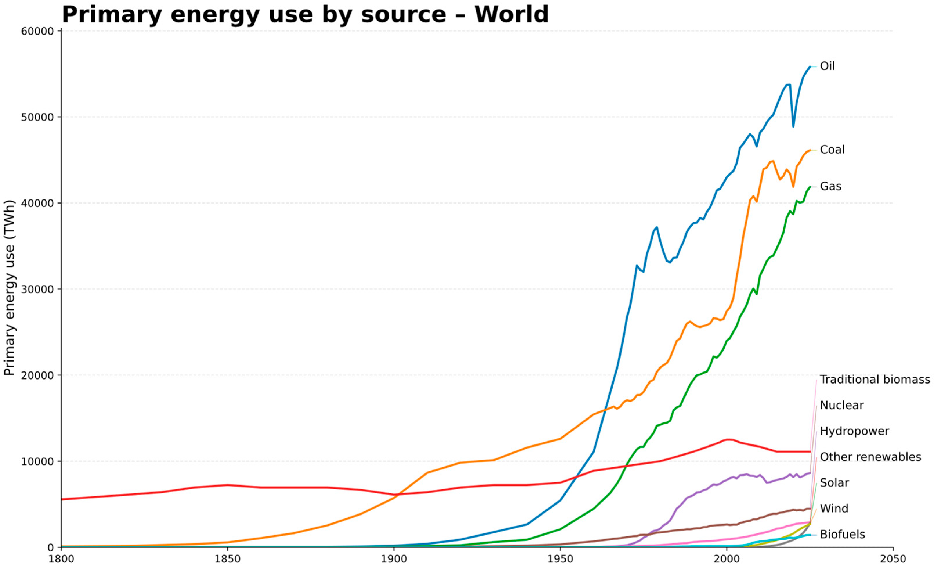
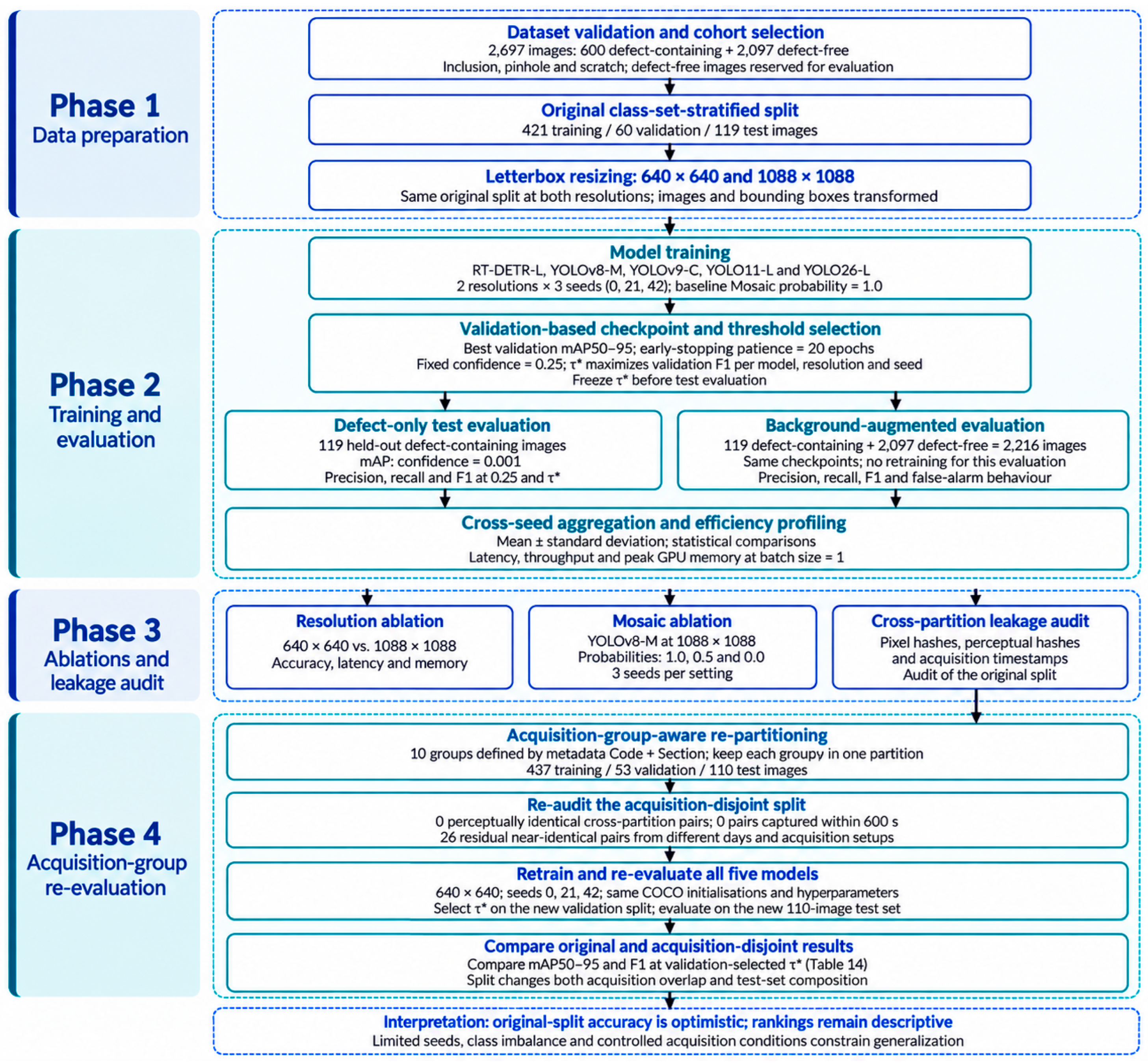
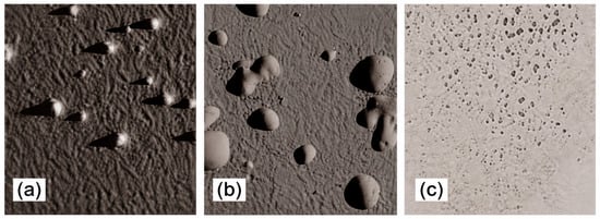
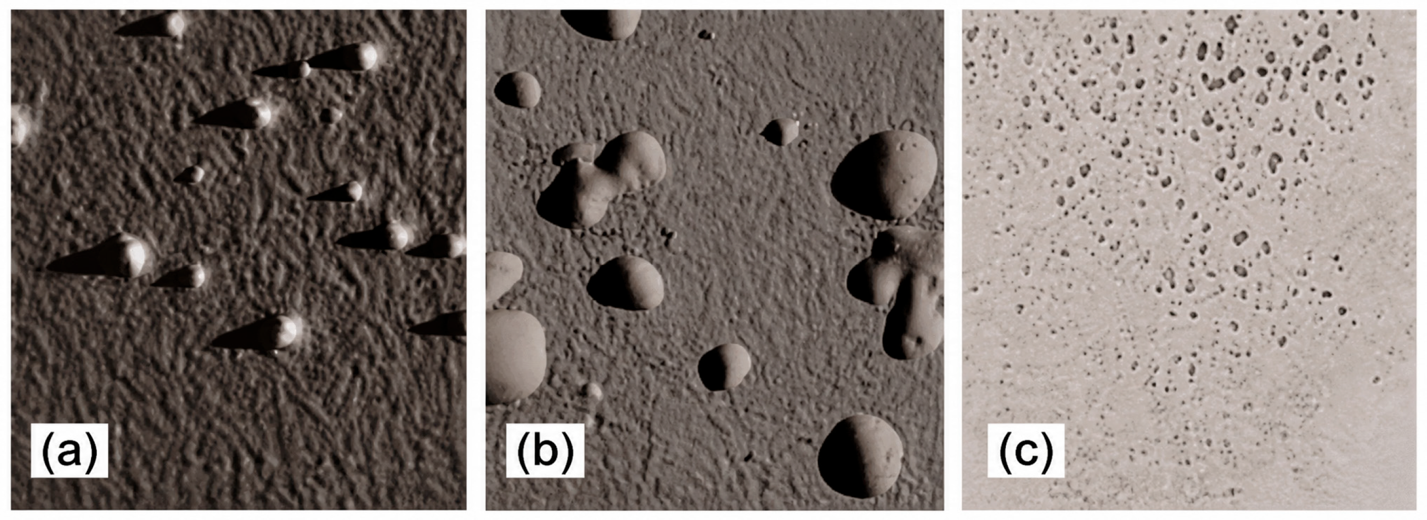
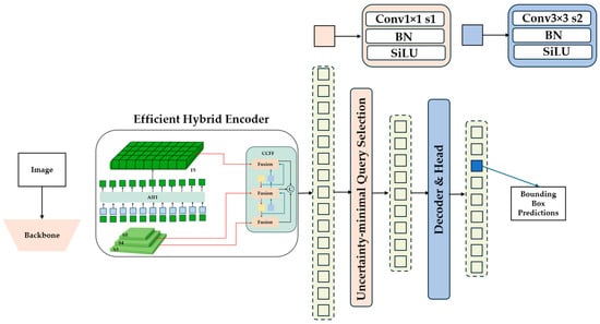
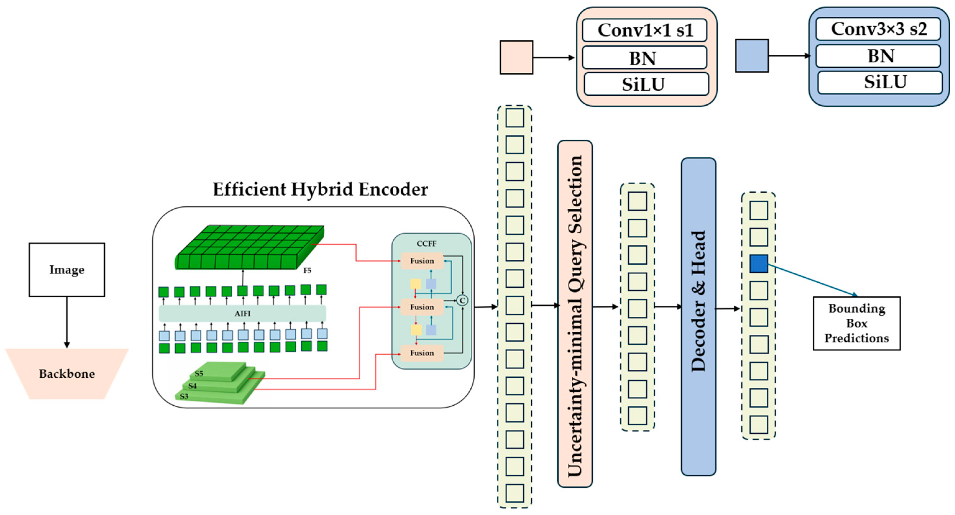
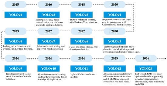
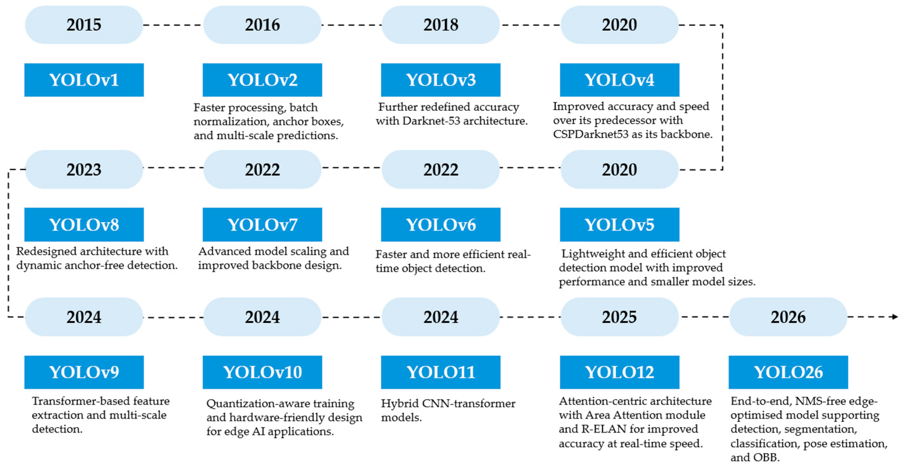
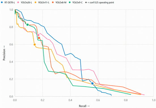
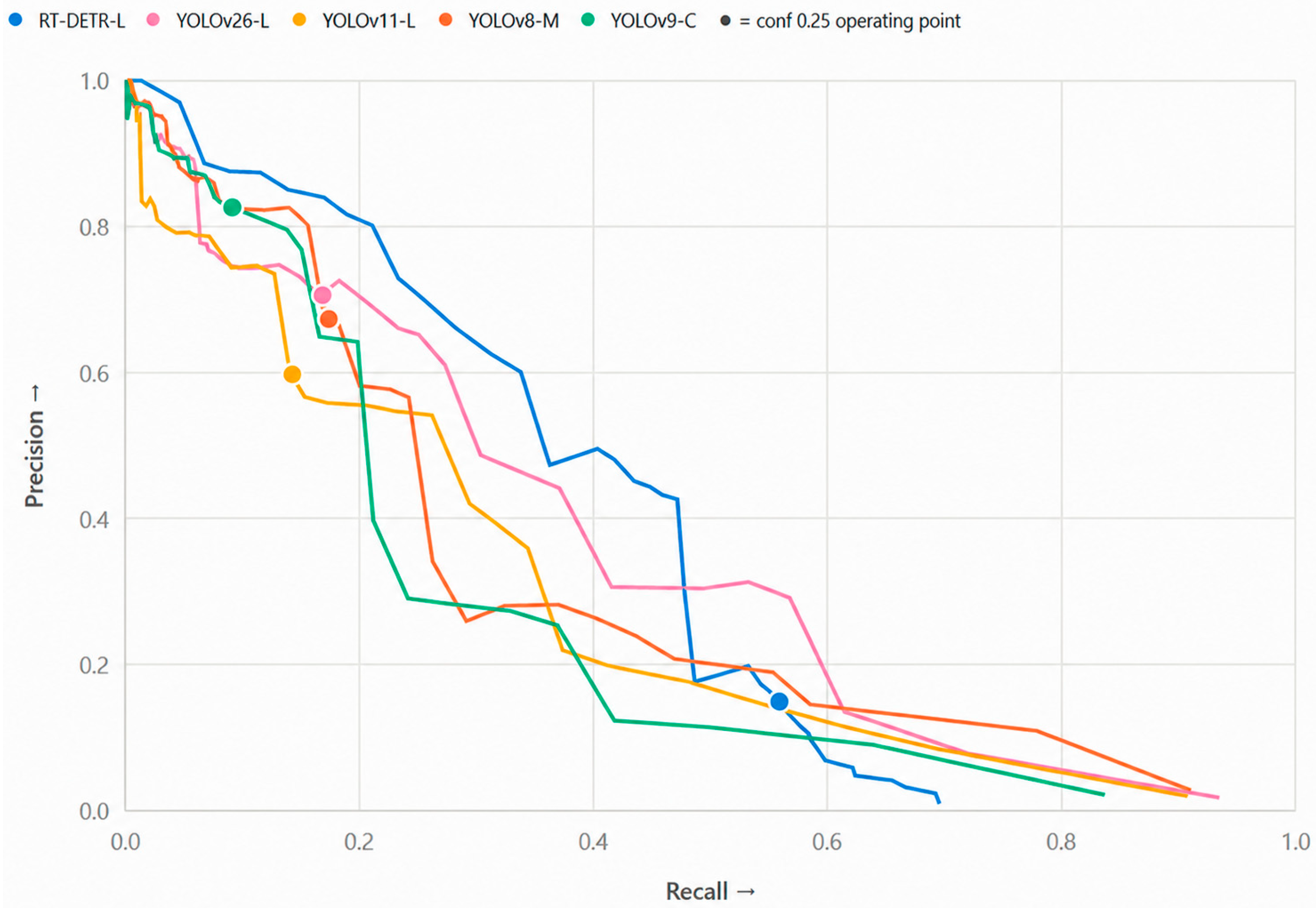
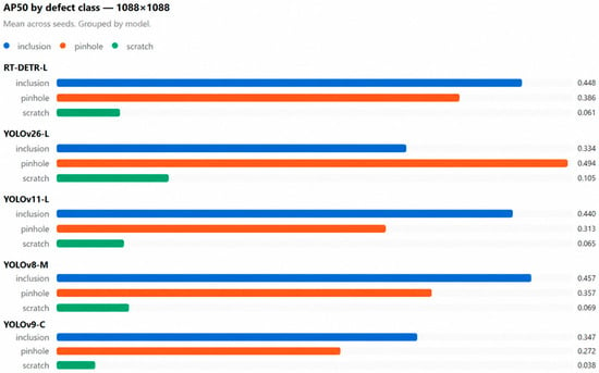
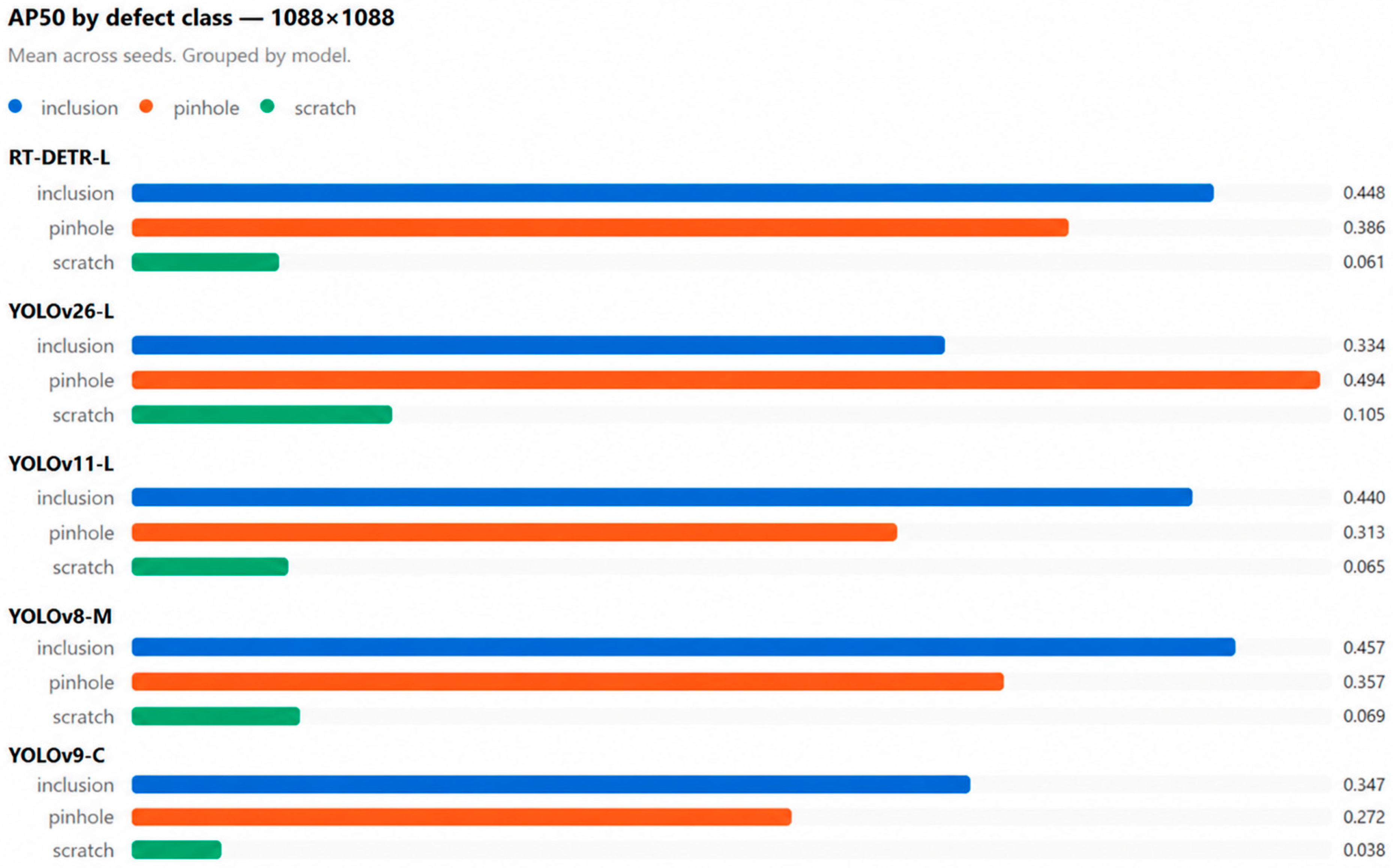
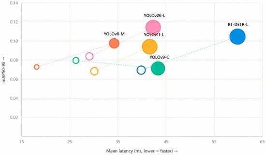
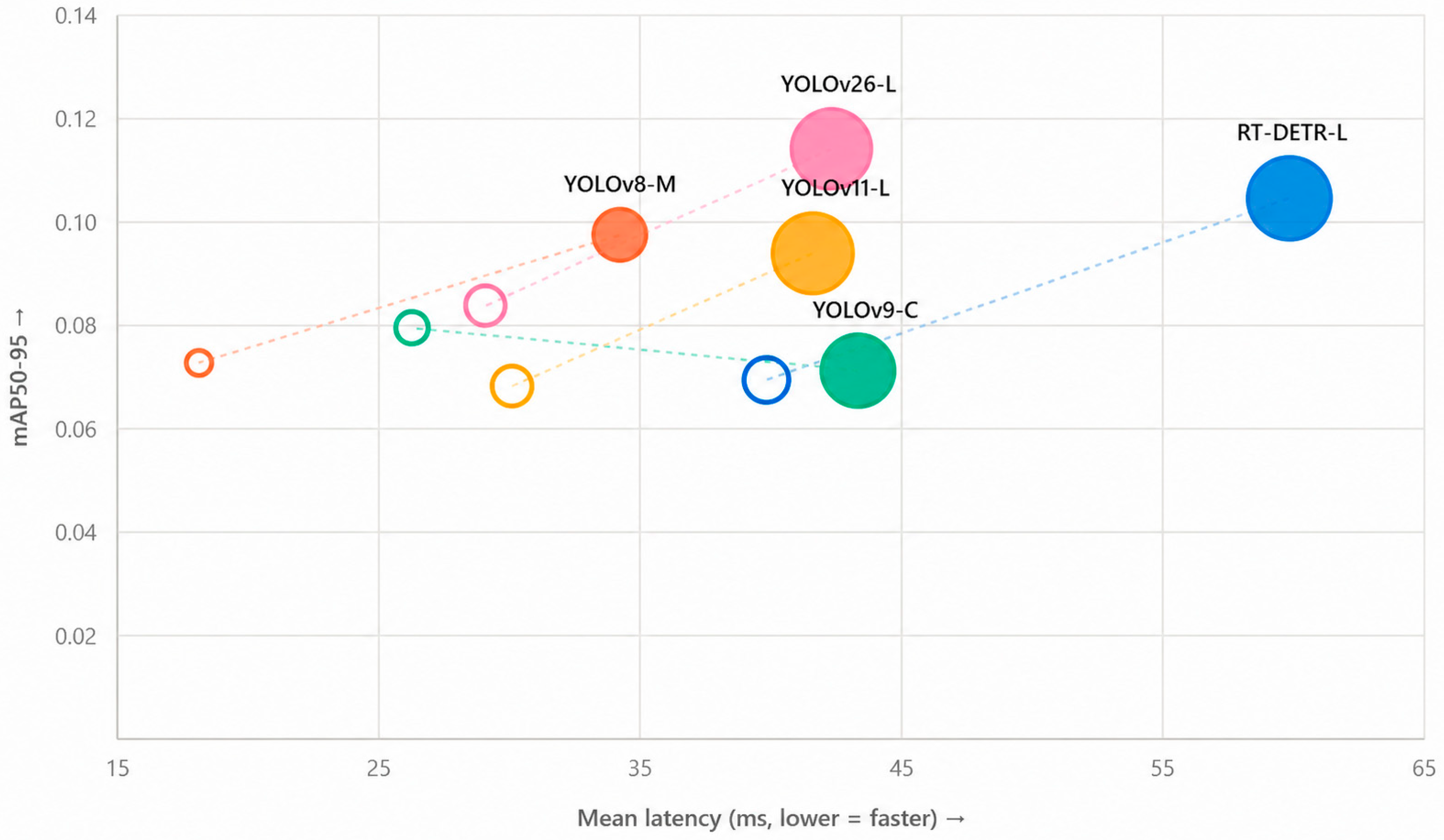
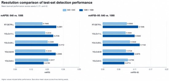
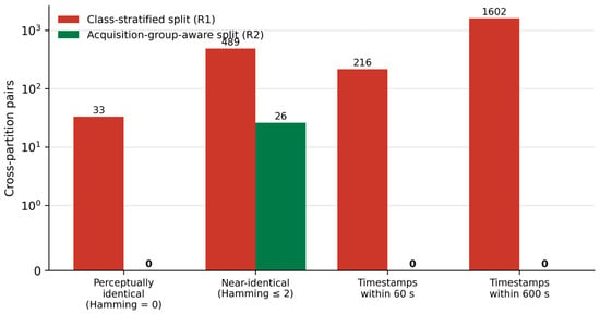
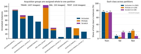
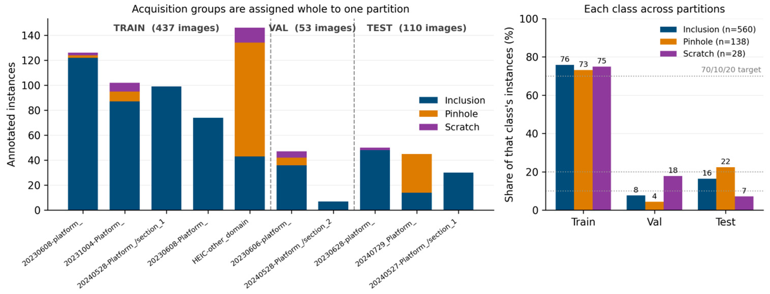

Disclaimer/Publisher’s Note: The statements, opinions and data contained in all publications are solely those of the individual author(s) and contributor(s) and not of MDPI and/or the editor(s). MDPI and/or the editor(s) disclaim responsibility for any injury to people or property resulting from any ideas, methods, instructions or products referred to in the content. |
© 2026 by the authors. Licensee MDPI, Basel, Switzerland. This article is an open access article distributed under the terms and conditions of the Creative Commons Attribution (CC BY) license.