


Abstract
Small unmanned aerial vehicle (UAV) acoustic signatures are relevant to environmental noise assessment, passive monitoring, and preliminary detectability analysis. This study presents a physics-informed reduced-order framework that combines blade-passing frequency (BPF) harmonic synthesis, rotational-speed acoustic scaling, propagation, and signal-to-noise ratio (SNR) threshold crossing. The RPM–OASPL law was calibrated using ten digitized measurements for a four-rotor DJI Phantom II with Original 9450 propellers and validated, without refitting, against eleven Aftermarket 9443 measurements. The fitted exponent was m = 5.285, and the fitted reference level was Lref = 77.01 dB(A) at 5000 RPM and 1 m. A 100,000-realization Monte Carlo analysis that propagated ±100 RPM and ±0.5 dB digitization bounds, together with residual scatter, produced total 95% intervals of 5.01–5.55 for m and 76.58–77.43 dB(A) for Lref. Calibration yielded RMSE = 0.39 dB and R2 = 0.9979; independent-configuration validation yielded MAE = 2.27 dB, RMSE = 2.38 dB, and R2 = 0.9168. At 5000 RPM, nominal free-field threshold-crossing distances were 70.9, 22.4, and 7.1 m for quiet rural, semi-urban, and urban scenarios. Combined statistical 95% screening intervals were 41.3–121.7, 13.0–38.5, and 4.1–12.2 m, respectively. Sensitivity analyses show that β controls harmonic-specific range but not normalized OASPL, while ground interference, band-limited masking, and detector processing can materially change operational range. The framework is therefore a rapid, interpretable screening tool rather than a universal detector performance model.
1. Introduction
The rapid proliferation of multirotor unmanned aerial vehicles has intensified interest in propeller-generated noise because it affects community acceptance, urban air mobility, environmental assessment, and passive surveillance. Small UAV spectra commonly contain blade-passing frequency tones and harmonics superimposed on broadband contributions from boundary-layer turbulence, wake interaction, motors, and airframe coupling. These tonal features can remain detectable even when the overall level approaches the ambient background.
The physical mechanisms are shared with other rotating-blade systems. Loading noise has a predominantly dipole character, thickness noise has a monopole character, and turbulence-related self-noise contributes broadband energy [1,2,3]. Blade-passing frequency forcing and dipole-like source behavior are also central to centrifugal pumps and other fluid machinery [4,5]. These cross-domain similarities support the use of compact harmonic and scaling models, while the differences in medium, confinement, blade loading, and rotor–stator interaction prevent direct transfer of fitted coefficients.
Existing UAV studies span high-fidelity CFD/FW–H calculations, controlled wind-tunnel measurements, field measurements, analytical source-mode models, and semi-empirical airfoil-noise formulations [2,6,7,8,9,10,11,12,13,14,15]. Analytical source-mode approaches can efficiently predict tonal radiation for prescribed rotor loading, whereas BPM/NACA-type formulations estimate broadband airfoil self-noise from aerodynamic boundary-layer quantities. These methods are more physically detailed than a two-parameter RPM law but require geometry, loading, or flow information that is rarely available during early screening.
A different literature focuses on passive detection and classification using spectral features, neural networks, distributed microphone arrays, and RF–acoustic fusion [16,17,18,19,20,21,22]. Those systems convert sensor data into detection or classification decisions, but their reported range depends on sensor bandwidth, array gain, training data, false-alarm constraints, and the ambient spectrum. Consequently, source-noise studies often stop before detectability, while detector studies often lack a transparent source-to-receiver model.
The present contribution does not claim a new fundamental acoustic law. Its novelty is the reproducible integration of known elements: BPF harmonic representation, a physically interpretable RPM power law, uncertainty propagation, free-field and two-ray propagation sensitivity, and broadband/tonal SNR thresholding within one calibrated screening workflow. This combination links an emitted source level to a conditional detection-distance estimate and explicitly separates calibration uncertainty, cross-configuration error, and environmental sensitivity.
Potential uses include rapid comparison of operating RPM, early iteration of low-observability rotor concepts, preliminary sensor placement, and first-order assessment of multiple-UAV or swarm scenarios. For several vehicles, energy summation may provide a screening bound only when source coherence and geometry are specified; coherent reinforcement, asynchronous rotors, and spatial separation require a dedicated array/propagation model and are not resolved here.
The principal contributions are: (i) a unit-consistent harmonic source representation using pressure amplitudes and mean-square-pressure summation; (ii) calibration and independent-configuration validation of an RPM–OASPL power law; (iii) Monte Carlo propagation of digitization and regression uncertainty; (iv) quantitative sensitivity of harmonic roll-off, atmospheric absorption, two-ray ground interference, and broadband versus tonal detection; (v) explicit similarity bounds using tip Mach number, thrust coefficient, blade count, rotor count, and operating condition; and (vi) a computationally inexpensive implementation suitable for real-time or embedded screening.
The calibration uses the four-rotor static-thrust measurements of Intaratep et al. [6]. The Original 9450 configuration is used for fitting and the Aftermarket 9443 configuration is reserved for validation without refitting. Because both datasets come from the same vehicle family and campaign, the validation is configuration-level rather than universal. Forward flight, markedly different propeller geometries, rotor counts, and sensor-processing chains require additional data or refitting.
2. Materials and Methods
2.1. Overview and Scope
The reduced-order workflow contains four coupled modules:
(1) BPF harmonic synthesis;
(2) experimentally calibrated RPM–OASPL scaling;
(3) source-to-receiver propagation;
and (4) SNR-based threshold crossing.
The model is intended for rapid comparative assessment and uncertainty-aware screening. It does not reproduce three-dimensional acoustic fields, waveform-level rotor phase, microphone-array beamforming, false-alarm probability, or classifier performance.
The calibrated source level represents the complete measured four-rotor vehicle at a fixed observer orientation. Therefore, motor/ESC noise and rotor–rotor interaction present in the experiment are implicitly included in the fitted OASPL trend, but they are not separately identified. The method does not obtain a four-rotor level by simply adding four isolated-rotor spectra, and it should not be transferred to another rotor count without a new acoustic anchor.
2.2. Unit-Consistent Harmonic Source Model
For B blades per rotor and rotational speed Ω in revolutions per minute, the blade-passing frequency is
where is in hertz. The screening spectrum is evaluated on discrete frequency bins . Broadband and tonal components are added in mean-square pressure space:
Here, is a relative mean-square pressure quantity, is the broadband contribution, is a dimensionless Gaussian line shape centered at n and normalized over the frequency grid, and is an rms pressure amplitude. Equation (2) no longer uses a Dirac delta and does not add spectral density to discrete pressure amplitudes.
Harmonic pressure amplitudes follow
so the relative level of harmonic n is . The factor 20 is used because is a pressure amplitude; the squared amplitudes are summed as energy in Equation (2). The discretized spectrum is normalized to the independently calibrated overall level :
The baseline uses and β = 0.60. Because raw narrowband data were unavailable, β is not treated as universal. A global sweep from 0.50 to 0.70 quantifies its influence on individual harmonics and narrowband range. Normalization in Equation (4) keeps total OASPL fixed; therefore, β redistributes tonal energy rather than changing the calibrated broadband total.
2.3. Rotational-Speed Acoustic Scaling and Model Selection
For a fixed diameter and broadly similar loading, tip speed is proportional to RPM. If the radiated mean-square pressure or acoustic power follows a velocity power law, the dB-domain relationship is logarithmic:
where is the A-weighted level referenced to 1 m, , is the fitted level at , and m is the acoustic-energy scaling exponent. For a fixed diameter, m also represents the exponent with respect to tip speed. Loading-dominated rotor noise is commonly associated with approximately sixth- to eighth-power Mach number trends under idealized similarity conditions [23,24]; mixed broadband/tonal content, A-weighting, changing loading, and motor contributions can shift an experimentally fitted OASPL exponent.
The logarithmic law was selected before examining validation results because it is monotonic, physically interpretable, and linear in its two fitted coefficients. A raw linear RPM model and a quadratic RPM model were also evaluated. Neural networks were not trained because ten calibration points are insufficient to estimate a stable data-driven model or conduct independent hyperparameter selection. Bayesian optimization would not improve the closed-form global optimum of this two-parameter least-squares problem; such methods become relevant only for multi-configuration, nonlinear, or high-dimensional calibration.
Calibration data were digitized from Figures 5 and 12 in the study by Intaratep et al. [6]. Rotor-speed versus thrust and OASPL versus thrust curves were combined to obtain ten Original 9450 RPM–OASPL pairs from 2000 to 6500 RPM. Measured levels at the 1.51 m slant distance were converted to a 1 m reference by adding . Eleven Aftermarket 9443 points from 2000 to 7000 RPM were reserved for validation.
2.4. Monte Carlo Uncertainty Propagation
The conventional OLS intervals describe regression scatter but do not propagate figure-reading uncertainty. A 100,000-realization Monte Carlo analysis was, therefore, performed. In each realization, every digitized RPM was independently perturbed with a uniform distribution bounded by ±100 RPM, and every digitized OASPL value with a uniform distribution bounded by ±0.5 dB. Gaussian residual noise with a standard deviation equal to the baseline regression residual standard error was then added, and Equation (5) was refitted. The 2.5th and 97.5th percentiles were reported as total parameter intervals.
For detection-distance uncertainty, each Monte Carlo source prediction was additionally perturbed by a zero-mean Gaussian cross-configuration error with σ equal to the 2.38 dB validation RMSE. These combined statistical intervals do not include unknown wind, ground impedance, microphone directivity, ambient spectrum variation, or detector threshold uncertainty. Those effects are reported separately as sensitivity cases rather than being mislabeled as measured confidence intervals.
2.5. Propagation Model
The baseline received level uses spherical spreading and frequency-dependent atmospheric absorption:
where = 1 m, α(f) is the atmospheric absorption coefficient in dB/m, and is a ground-interference correction. The baseline tables set α = 0 and = 0 to preserve a transparent free-field reference. When α = 0 and = 0, the threshold distance is
Atmospheric absorption was calculated for an illustrative 20 °C, 70% relative-humidity, and 101.325 kPa atmosphere using the ISO 9613-1 formulation [25]. Ground interference was illustrated with a two-ray expression:
where Γ is the complex ground-reflection coefficient, and are the direct and reflected path lengths, and k is the acoustic wavenumber. Because Γ depends on frequency, angle, impedance, and moisture, the two-ray case is a sensitivity illustration rather than a site-specific correction. Atmospheric refraction and wind gradients are not modeled; they require meteorological profiles and ray-tracing or parabolic equation methods.
2.6. Broadband and Tonal SNR Thresholds
Broadband threshold crossing is defined by
with = 5 dB. Representative broadband ambient levels of 35, 45, and 55 dB(A) produce effective thresholds of 40, 50, and 60 dB(A). These values are scenarios, not universal standards.
A tonal detector evaluates a BPF line or narrow frequency band rather than total A-weighted energy:
where is the processing gain from spectral-line integration or matched filtering. To show why tonal processing is not automatically superior, an explicit semi-urban illustration uses = − 6 dB, a 160 Hz one-third-octave ambient level 8 dB below broadband ambient, and optional = 6 dB. These assumptions are transparent sensitivity inputs, not calibrated detector data. A second case sets the band ambient equal to broadband ambient to represent low-frequency masking.
The model reports threshold-crossing distance, not probability of detection. A task-oriented sensing chain would additionally include acquisition, preprocessing, feature extraction, detection/classification, confidence estimation, and sensor fusion [26]. Such data-driven stages complement the present physical screening model but cannot be inferred from OASPL alone.
2.7. Parameters and Computational Implementation
The implementation was executed in Python 3.13.5 (Python Software Foundation, Wilmington, DE, USA) and performs data normalization, least-squares calibration, model comparison, Monte Carlo propagation, validation, harmonic synthesis, propagation sensitivity, and range estimation. The core analytic calculation is vectorized and evaluates 10,000 RPM threshold cases in a median of 1.3 ms in the test environment, excluding file input/output and plotting. This low cost supports embedded or real-time screening, although real sensor pipelines will be dominated by signal acquisition and spectral processing. The complete reproducible implementation and the correspondence of Supplementary Files S1–S6 are described in Appendix A. The ambient scenarios and corresponding effective thresholds are summarized in Table 1, and the baseline parameters and calibration domain are listed in Table 2.
Table 1.
Ambient levels, nominal SNR margin, and broadband effective thresholds.
Table 2.
Baseline model parameters and calibration domain.
2.8. Validation and Applicability Criteria
Calibration performance was assessed with MAE, RMSE, R2, maximum absolute error, AICc, and leave-one-out cross-validation (LOOCV). Predictive transfer was assessed on the reserved Aftermarket 9443 dataset without changing m or . The free-field propagation slope was checked against the approximately 6 dB per distance doubling reported by Kloet et al. [27].
Direct use without refitting is limited to configurations near the calibration domain: four rotors, two blades per rotor, approximately 0.239 m diameter, 2000–6500 RPM, tip Mach 0.073–0.237, and per-rotor static-thrust coefficient 0.120–0.142. The Aftermarket 9443 validation supports modest changes within the same 9.4-inch propeller family. Three-bladed propellers, substantially different diameters/camber, other rotor counts, ducted/coaxial systems, and forward-flight advance ratios require at least a new reference measurement and preferably a new calibration. Hover or quasi-hover use beyond μ = 0 remains an extrapolation, not a validated domain. Additional details regarding the scope, assumptions, and limitations of the proposed framework are provided in Appendix B.
3. Results
3.1. Harmonic Spectrum and β Sensitivity
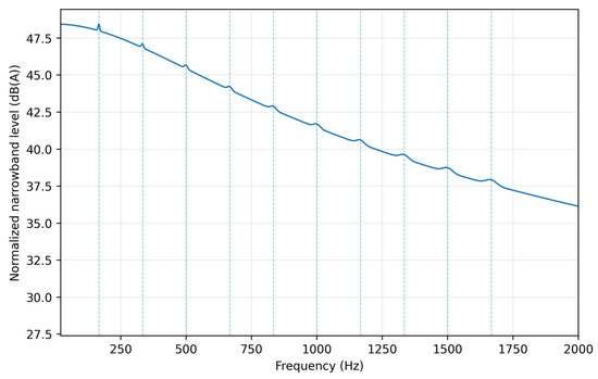
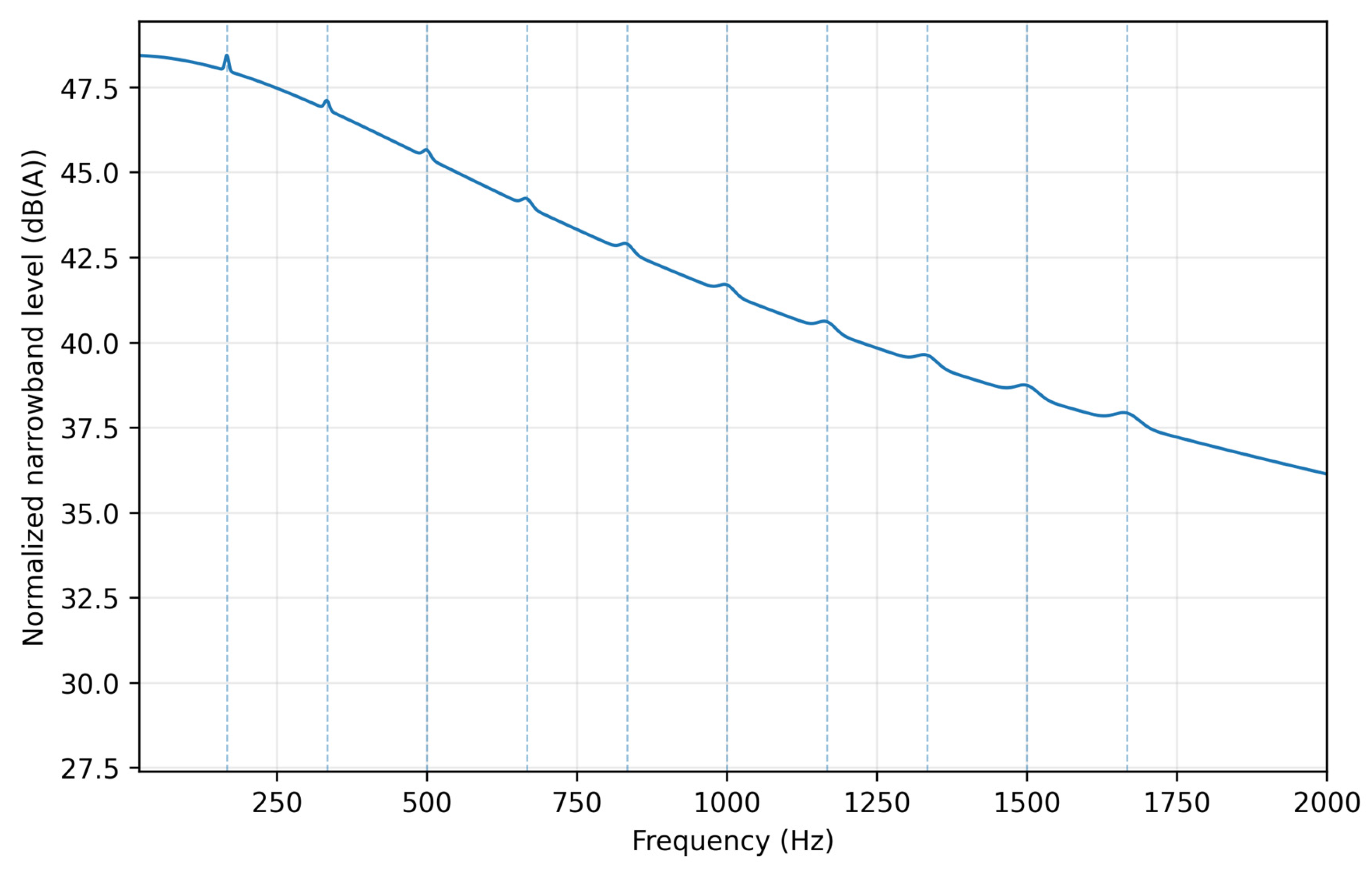
At 5000 RPM with two blades, the fundamental BPF is 166.7 Hz. Figure 1 shows the normalized screening spectrum with ten BPF-centered Gaussian components. The plotted ordinate is a normalized narrowband level, whose energy sum equals the fitted 77.01 dB(A) total; it is not a measured power spectral density or waveform reconstruction.
Figure 1.
Normalized screening spectrum at 5000 RPM. Dashed lines identify the first ten BPF harmonics; the spectrum is energy-normalized to the calibrated OASPL and is not a substitute for measured narrowband data.
The β sweep gives first-to-tenth-harmonic pressure-level reductions of 10, 12, and 14 dB for β = 0.50, 0.60, and 0.70. Because the narrowband range is proportional to pressure amplitude under identical propagation and band noise, the tenth-harmonic range is 0.316, 0.251, or 0.200 times the fundamental range. The full 0.50–0.70 interval therefore changes the tenth-harmonic range by a factor of 1.58, even though the normalized total OASPL is unchanged. The quantitative harmonic-level and range ratios are summarized in Table 3.
Table 3.
Global sensitivity of harmonic level and harmonic-specific range to β.
3.2. RPM–OASPL Calibration, Physical Scaling, and Model Selection
The logarithmic fit produced at 5000 RPM and , equivalent to a 52.85 dB-per-decade slope. The measured 5000 RPM checkpoint is 77.216 dB(A); is the fitted regression value at the reference RPM and is not constrained to equal that single observation. Their 0.206 dB difference is the residual at the reference point.
The exponent implies that acoustic mean-square pressure scales approximately as and rms pressure as within the calibration domain. This is physically compatible with a loading-dominated trend of order six while remaining lower than idealized sixth- to eighth-power Mach number laws, as expected for A-weighted total noise containing changing load, broadband noise, and motor contributions.
The raw linear model produced RMSE = 1.27 dB and LOOCV RMSE = 1.71 dB. A quadratic model reduced in-sample RMSE to 0.33 dB but had essentially the same LOOCV error as the logarithmic law and a less favorable AICc because of the extra parameter. The logarithmic model, therefore, provides the best balance of calibration fit, parsimony, monotonicity, and physically defensible extrapolation within the stated domain. The comparison metrics are summarized in Table 4.
Table 4.
Comparison of candidate RPM–OASPL relationships using the ten calibration points.
The conventional OLS intervals were 5.09–5.48 for m and 76.64–77.38 dB(A) for . After propagating digitization bounds and residual scatter, the total Monte Carlo 95% intervals widened to 5.01–5.55 and 76.58–77.43 dB(A). The central values remained stable, indicating that the power-law calibration is not driven by small digitization perturbations.
3.3. Calibration and Independent-Configuration Validation
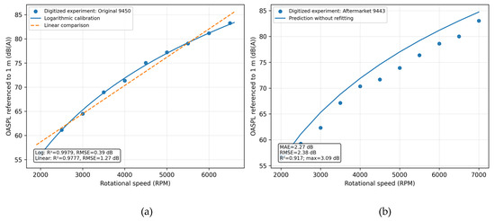
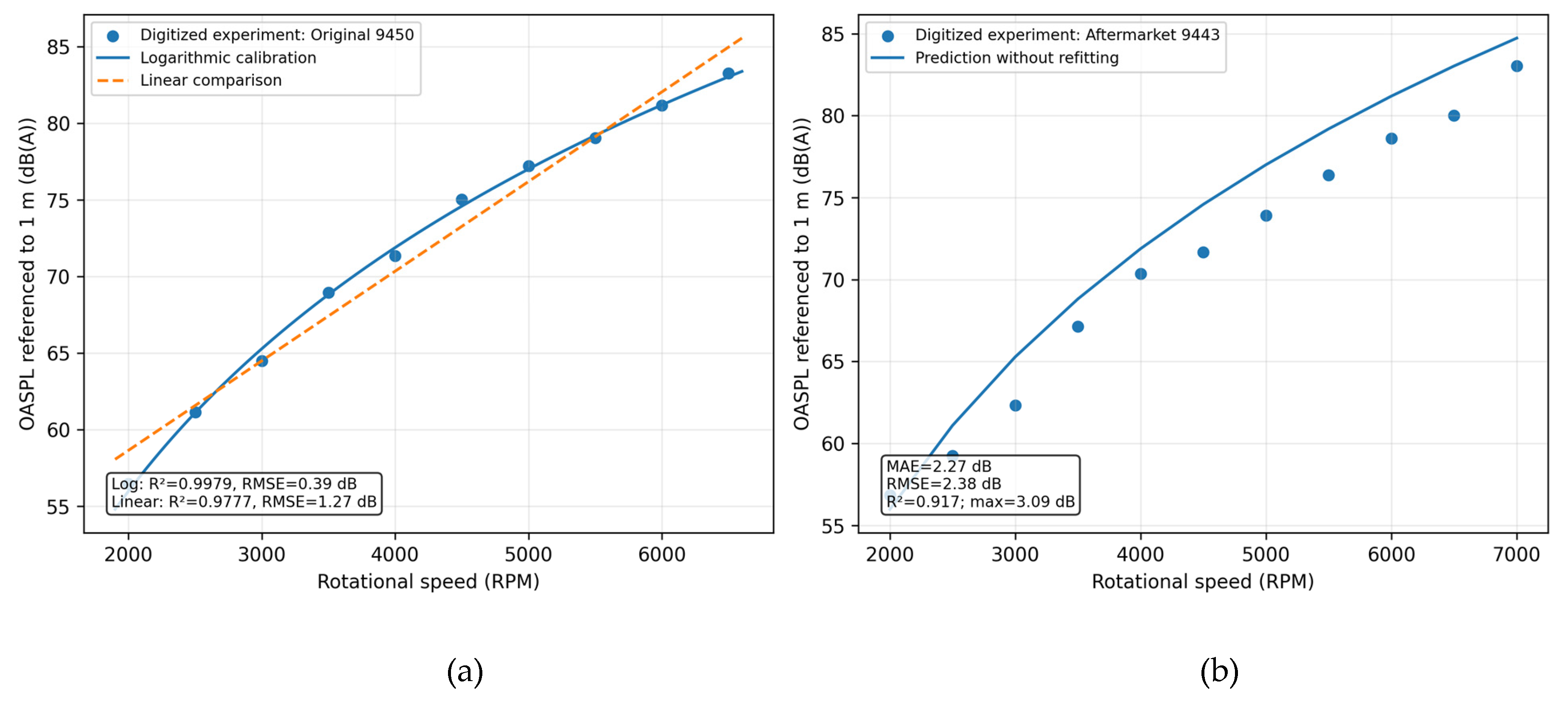
Across the ten Original 9450 points, the logarithmic model achieved MAE = 0.31 dB, RMSE = 0.39 dB, R2 = 0.9979, and maximum error = 0.80 dB. The calibration results are shown in Figure 2a. Applied without refitting to the eleven Aftermarket 9443 points, it achieved MAE = 2.27 dB, RMSE = 2.38 dB, R2 = 0.9168, maximum error = 3.09 dB, and measured-minus-predicted bias = −2.11 dB. Figure 2b, therefore, shows useful trend transfer but also a systematic source-level offset that must be retained in range uncertainty. Representative experimental checkpoints and fitted Original 9450 levels are listed in Table 5.
Figure 2.
RPM–OASPL credibility assessment: (a) Original 9450 calibration, including the raw linear benchmark; (b) Aftermarket 9443 prediction without refitting. The systematic negative validation residual indicates that the Original 9450 calibration overpredicts the quieter Aftermarket 9443 configuration.
Table 5.
Experimental checkpoints and fitted Original 9450 levels at 1 m.
3.4. Broadband Threshold-Crossing Distances and Statistical Intervals
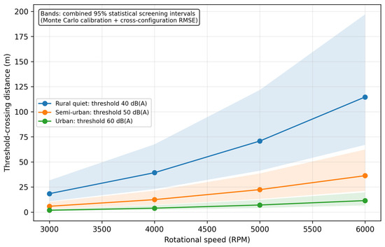
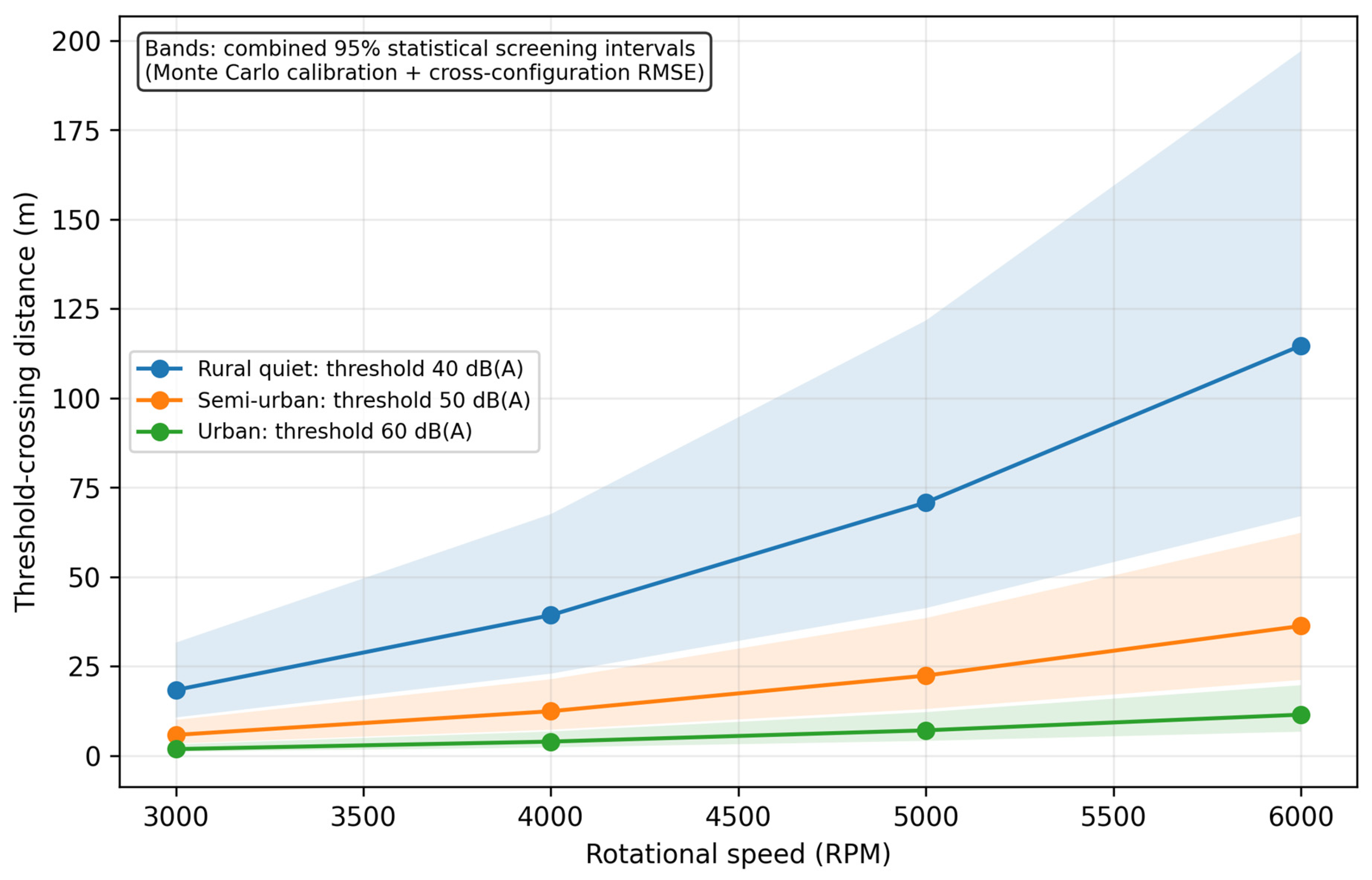
Figure 3 and Table 6 combine Monte Carlo calibration uncertainty with the external-validation RMSE under a Gaussian cross-configuration error assumption. These are statistical screening intervals, not guaranteed operational sensor ranges. Environmental and detector sensitivities are presented separately.
Figure 3.
Free-field broadband threshold-crossing distance versus RPM. Shaded bands combine Monte Carlo calibration uncertainty and the 2.38 dB independent-configuration RMSE; they exclude unknown ground, meteorological, directivity, and detector-threshold effects.
Table 6.
Nominal broadband threshold-crossing distances, with combined statistical 95% screening intervals in brackets.
At 5000 RPM, the nominal distances are 70.9, 22.4, and 7.1 m. A 10 dB increase in the effective threshold reduces the free-field range by 68.4%. Conversely, an unmodeled ±3 dB directivity, microphone, or propagation correction changes the range by factors of 0.71–1.41; ±6 dB changes it by factors of 0.50–2.00. This environmental sensitivity is comparable to or larger than the calibration uncertainty.
3.5. Broadband Versus Tonal Detection Illustration
For the semi-urban 5000 RPM case, the broadband criterion gives 22.4 m. Under the stated illustrative assumptions, using a fundamental BPF line 6 dB below OASPL and a one-third-octave ambient level 8 dB below broadband ambient increases the no-processing-gain range to 28.2 m. Adding 6 dB line/matched-filter processing gain increases it to 56.3 m. However, when low-frequency band noise equals the broadband ambient level, the same tone reaches only 11.2 m. Tonal processing can therefore extend the range by order-unity factors, but only when the BPF band has favorable noise and detector gain.
3.6. Atmospheric, Ground, and Applicability Sensitivity
At 20 °C and 70% relative humidity, ISO 9613-1 [25] absorption over 100 m is approximately 0.37 dB at 166.7 Hz and 0.46 dB at 1 kHz. Atmospheric absorption is therefore modest at these frequencies and ranges, although it increases at higher harmonics and longer paths. Ground interference can be larger and oscillatory.
For an illustrative 100 m direct path at a 30° elevation, a 1.5 m receiver, a 51.5 m source, and a real reflection coefficient Γ = 0.5, the two-ray correction is +0.84 dB at the fundamental BPF, −5.86 dB at the second BPF, and −5.61 dB at 1 kHz. These values demonstrate frequency-selective reinforcement and cancellation; they are not a universal grassy-ground correction because real Γ is complex and site-dependent.
The validated similarity domain is narrow but explicit: four rotors, two blades, 0.239 m diameter, static thrust, tip Mach 0.073–0.237, and C_T = 0.120–0.142. Within the same propeller family, the transfer error was 2–3 dB. No evidence in the present dataset establishes accuracy for three-bladed propellers, other diameters, forward flight, strongly different camber, coaxial/ducted rotors, or other vehicle classes.
4. Discussion
The principal result is not merely the high calibration R2, which is expected for a smooth ten-point trend, but the combination of physically interpretable scaling, independent-configuration error, and propagated range uncertainty. The fitted m = 5.285 is consistent in order with loading-dominated rotor scaling. It should not be interpreted as a universal Lighthill exponent; the present OASPL combines dipole loading noise, broadband self-noise, possible motor tones, A-weighting, and changing thrust across RPM.
Compared with analytical source-mode models and BPM/NACA-type semi-empirical methods, the proposed framework needs substantially fewer geometric and aerodynamic inputs and directly produces a conditional detection distance. The cost is reduced spectral and directional fidelity. Compared with CFD/FW–H, it avoids meshing and time marching and evaluates thousands of cases in milliseconds, but it cannot resolve blade loading, rotor–rotor wake interaction, directivity, or installation effects. The 2.38 dB external-validation RMSE provides a quantitative accuracy scale for a similar propeller; no matched dataset is available to claim superiority over high-fidelity methods.
The β analysis clarifies the role of harmonic decay. Because total OASPL is normalized independently, β does not affect broadband distances in Table 6. It can, however, change higher-harmonic line range by tens of percent. A universal β cannot be defended from a single digitized spectrum; future work requires raw narrowband measurements from multiple blade counts, diameters, loading coefficients, and observer angles.
The broadband/tonal comparison also resolves an apparent contradiction. Broadband A-weighted thresholds may be conservative when the BPF band is quieter than the total ambient spectrum and the detector provides line-processing gain. They may be optimistic when urban low-frequency masking overlaps the BPF. Operational use, therefore, requires measured one-third-octave or narrowband ambient spectra, detector bandwidth, array gain, integration time, and false-alarm constraints.
Ground effects should not be described merely as random scatter. The two-ray illustration shows a known frequency-dependent sign: direct and reflected paths can reinforce or cancel. Consequently, the free-field values are conditional reference estimates rather than universal upper bounds. Depending on phase and ground impedance, a free-field estimate can overpredict or underpredict a specific tonal level. Atmospheric refraction and wind gradients can further alter low-altitude paths and require meteorological data.
Generalizability remains the main limitation. The Aftermarket 9443 validation is independent of fitting but belongs to the same vehicle family and campaign. The model should therefore be anchored with at least one matched measurement for a new vehicle. In forward flight, nonuniform inflow changes blade loading and directivity; experimental UAV-rotor studies show pronounced BPF asymmetry and Mach number dependence with advance ratio [24]. Rotor–rotor phase and wake interaction are implicitly embedded only for the calibrated Phantom II geometry.
Machine learning was deliberately not added to the present calibration. With ten training points, a neural network, transfer-learning model, PINN, or Bayesian optimizer would add unidentifiable parameters and a high risk of overfitting. For a future multi-UAV database, data-driven surrogates could map geometry and operating state to acoustic parameters, while physical equations could regularize predictions. Cross-domain CFD-trained CNN surrogates demonstrate the potential of this strategy in complex flow systems [28], but they do not validate UAV acoustics and are cited only as a methodological example.
A task-oriented detection architecture could combine the present source/range prior with microphone-array features, machine learning classification, and RF/optical fusion [18,21,26]. Transfer learning may reduce calibration cost for new propeller families, and PINN-type regularization could enforce propagation or FW–H-inspired constraints. These are future extensions, not missing components that can be credibly trained from the current dataset.
Motor electromagnetic and ESC switching noise are not separated. Because calibration uses whole-vehicle OASPL, such contributions are partly embedded in L_ref and m. At low RPM, motor tones may become proportionally important, and the aerodynamic BPF model may underestimate or misattribute spectral peaks. Dedicated motor-on/propeller-off and rotor-only measurements are needed to decouple these sources.
The uncertainty analysis is intentionally layered. The Monte Carlo interval addresses digitization and regression scatter; the validation RMSE addresses transfer to a similar propeller; Table 7 and Table 8 address detector and environmental sensitivity. A single ‘total operational 95% confidence interval’ cannot be justified without probability distributions for ground impedance, weather, directivity, ambient spectra, and detector thresholds. Reporting a falsely precise total interval would be less rigorous than separating measured statistical uncertainty from scenario sensitivity.
Table 7.
Illustrative 5000 RPM semi-urban comparison of broadband and BPF-line threshold crossing.
Table 8.
Quantitative propagation illustration for a 100 m path at 20 °C and 70% relative humidity.
5. Conclusions
This study developed a calibrated reduced-order framework for small-UAV acoustic signature and passive threshold-crossing screening. The main conclusions are:
- The logarithmic RPM law is physically interpretable and parsimonious. It achieved RMSE = 0.39 dB and R2 = 0.9979, while m = 5.285 is compatible in order with loading-dominated rotor scaling.
- Monte Carlo propagation of ±100 RPM, ±0.5 dB, and residual scatter widened the total 95% intervals to 5.01–5.55 for m and 76.58–77.43 dB(A) for L_ref without materially shifting the central estimates.
- Validation on the reserved Aftermarket 9443 configuration yielded MAE = 2.27 dB, RMSE = 2.38 dB, and R2 = 0.9168. This supports comparative screening within a similar propeller family, not universal prediction across UAV classes.
- At 5000 RPM, nominal free-field broadband distances were 70.9, 22.4, and 7.1 m for rural, semi-urban, and urban scenarios; combined statistical 95% screening intervals were 41.3–121.7, 13.0–38.5, and 4.1–12.2 m.
- β = 0.50–0.70 changes first-to-tenth-harmonic decay from 10 to 14 dB and changes tenth-harmonic-specific range by a factor of 1.58, while normalized total OASPL remains fixed.
- Tonal processing can extend range when band noise is low and processing gain is available, but low-frequency masking can make tonal range shorter than broadband range. Detector bandwidth and ambient spectra are, therefore, essential operational inputs.
- Atmospheric absorption near 1 kHz is modest over 100 m under the illustrated conditions, whereas ground interference can produce several decibels of reinforcement or cancellation. Free-field results are conditional reference values, not guaranteed upper bounds.
- The method is computationally suitable for real-time screening, but new rotor counts, blade numbers, diameters, forward-flight conditions, and vehicle families require matched measurements, broader validation, or higher-fidelity modeling.
Future work should prioritize raw multi-configuration spectra, controlled motor/rotor source separation, forward-flight and outdoor measurements, frequency-dependent ground and atmospheric propagation, sensor-specific detection curves, and hierarchical physics-informed/data-driven calibration across UAV classes.
Supplementary Materials
The following supporting information can be downloaded at https://www.mdpi.com/article/10.3390/computation14080189/s1: Supplementary File S1: Python reduced-order computational implementation (computation_model_revision2.py); Supplementary File S2: Original 9450 calibration dataset; Supplementary File S3: Aftermarket 9443 validation dataset; Supplementary File S4: Machine-readable model summary; Supplementary File S5: β-sensitivity results; Supplementary File S6: Atmospheric-absorption and two-ray propagation-sensitivity results.
Author Contributions
Conceptualization, D.S.-H., G.U.-S. and G.R.-R.; methodology, D.S.-H., G.U.-S., B.R.-A., J.P.-O. and M.P.-O.; software, D.S.-H., J.M.-R., A.T.-E. and J.A.G.-N.; validation, D.S.-H., G.U.-S., F.A.D.-P. and C.H.-A.; formal analysis, D.S.-H., C.E.H.-B., L.I.L.-C. and J.R.G.-I.; investigation, D.S.-H., J.P.-O., M.P.-O., F.A.D.-P. and C.H.-A.; resources, G.R.-R., B.R.-A. and G.U.-S.; data curation, D.S.-H., J.M.-R. and A.T.-E.; writing—original draft preparation, D.S.-H.; writing—review and editing, D.S.-H., G.U.-S., G.R.-R., B.R.-A., J.P.-O., M.P.-O., J.M.-R., F.A.D.-P., C.H.-A., C.E.H.-B., A.T.-E., J.A.G.-N., L.I.L.-C. and J.R.G.-I.; supervision, G.U.-S. and B.R.-A.; project administration, D.S.-H. All authors have read and agreed to the published version of the manuscript.
Funding
This research received no external funding.
Data Availability Statement
The digitized calibration and validation tables, revised Python 3.13.5 implementation, Monte Carlo/model summary file, β-sensitivity table, propagation sensitivity table, and generated figures are provided as Supplementary Files S1–S6. The underlying experimental measurements remain attributable to Intaratep et al. [6].
Acknowledgments
The authors acknowledge the academic and technical support provided by the Centro de Estudios Superiores Navales and the Escuela Superior de Ingeniería Mecánica y Eléctrica of the Instituto Politécnico Nacional. The authors reviewed and approved the final text and take full responsibility for the content.
Conflicts of Interest
The authors declare no conflicts of interest.
Abbreviations
The following abbreviations are used in this manuscript:
| BPF | Blade-Passing Frequency |
| CFD | Computational Fluid Dynamics |
| DI | Detectability Index |
| FW-H | Ffowcs Williams–Hawkings |
| RPM | Revolutions Per Minute |
| OASPL | Overall A-Weighted Sound Pressure Level |
| SNR | Signal-to-Noise Ratio |
| SPL | Sound Pressure Level |
| UAV | Unmanned Aerial Vehicle |
Appendix A. Python Reduced-Order Computational Implementation
The complete revised implementation is provided as Supplementary File S1 (computation_model_revision2.py). It reproduces data normalization, calibration, model selection, Monte Carlo uncertainty propagation, validation, harmonic synthesis, broadband and tonal range illustrations, propagation sensitivity, tables, and figures.
Supplementary File S2 contains the Original 9450 calibration table; S3 contains the Aftermarket 9443 validation table; S4 contains the machine-readable model summary; S5 contains the β-sensitivity results; and S6 contains atmospheric and two-ray propagation sensitivities.
The supplementary implementation is intended for transparent reproduction of the screening-level calculations and should not be interpreted as a high-fidelity aeroacoustic solver.
Appendix B. Supplementary Notes on Model Scope
The calibrated framework is intended for preliminary acoustic signature and passive threshold-crossing screening. It combines a fitted RPM–OASPL law, simplified harmonic structure, conditional propagation, uncertainty separation, and broadband/tonal SNR criteria.
The framework does not include full CFD/FW–H simulation, matched raw spectral calibration, rotor–airframe or general rotor–rotor interaction, atmospheric refraction, site-specific ground impedance, realistic microphone directivity, false alarm probability, classifier performance, or full microphone-array beamforming. The 2.38 dB validation RMSE applies only to transfer between two similar propeller configurations in the same experimental campaign.
Broader generalization requires raw measurements from additional rotor counts, blade numbers, diameters, airfoils, observer angles, forward-flight states, and outdoor environments. For a new vehicle, at least one matched acoustic reference is recommended before absolute range estimates are used.
References
- Ffowcs Williams, J.E.; Hawkings, D.L. Sound Generation by Turbulence and Surfaces in Arbitrary Motion. Philos. Trans. R. Soc. Lond. A 1969, 264, 321–342. [Google Scholar] [CrossRef] [Scilit]
- Brooks, T.F.; Pope, D.S.; Marcolini, M.A. Airfoil Self-Noise and Prediction. In NASA Reference Publication 1218; NASA Langley Research Center: Hampton, VA, USA, 1989. [Google Scholar]
- Brentner, K.S.; Farassat, F. Modeling Aerodynamically Generated Sound of Helicopter Rotors. Prog. Aerosp. Sci. 2003, 39, 83–120. [Google Scholar] [CrossRef] [Scilit]
- Rzentkowski, G.; Zbroja, S. Experimental Characterization of Centrifugal Pumps as an Acoustic Source at the Blade-Passing Frequency. J. Fluids Struct. 2000, 14, 529–558. [Google Scholar] [CrossRef] [Scilit]
- Parrondo, J.; Pérez, J.; Barrio, R.; González, J. A Simple Acoustic Model to Characterize the Internal Low-Frequency Sound Field in Centrifugal Pumps. Appl. Acoust. 2011, 72, 59–64. [Google Scholar] [CrossRef] [Scilit]
- Intaratep, N.; Alexander, W.N.; Devenport, W.J.; Grace, S.M.; Dropkin, A. Experimental Study of Quadcopter Acoustics and Performance at Static Thrust Conditions. In Proceedings of the 22nd AIAA/CEAS Aeroacoustics Conference, Lyon, France, 30 May–1 June 2016. AIAA 2016-2873. [Google Scholar] [CrossRef] [Scilit]
- Ramos-Romero, C.; Green, N.; Torija, A.J. On-Field Noise Measurements and Acoustic Characterisation of Small Unmanned Aircraft Systems. Aerosp. Sci. Technol. 2023, 135, 108191. [Google Scholar] [CrossRef] [Scilit]
- Dbouk, T.; Drikakis, D. Computational Aeroacoustics of Quadcopter Drones. Appl. Acoust. 2022, 192, 108738. [Google Scholar] [CrossRef] [Scilit]
- Thai, A.D.; De Paola, E.; Di Marco, A.; Stoica, L.G.; Camussi, R.; Tron, R.; Grace, S.M. Experimental and Computational Aeroacoustic Investigation of Small Rotor Interactions in Hover. Appl. Sci. 2021, 11, 10016. [Google Scholar] [CrossRef] [Scilit]
- Schäffer, B.; Heutschi, K.; Hellweg, S. Drone Noise Emission Characteristics and Noise Effects on Humans—A Systematic Review. Int. J. Environ. Res. Public Health 2021, 18, 5940. [Google Scholar] [CrossRef] [Scilit] [PubMed]
- Pérez-Collazo, C.; Greaves, D.; Iglesias, G. Motor Noise Reduction of Unmanned Aerial Vehicles. Appl. Acoust. 2022, 196, 108882. [Google Scholar] [CrossRef] [Scilit]
- Zhou, W.; Ning, Z.; Li, H.; Hu, H. Aeroacoustic Analysis of Ducted Contra-Rotating Rotor Unmanned Aerial Vehicle. AIAA J. 2025, 63, 3261–3274. [Google Scholar] [CrossRef] [Scilit]
- Škultéty, F.; Kováčiková, K.; Pecho, P.; Kandera, B. Noise Impact Assessment of UAS Operation in Urbanised Areas. Drones 2023, 7, 314. [Google Scholar] [CrossRef] [Scilit]
- Roger, M.; Moreau, S. Tonal-Noise Assessment of Quadrotor-Type UAV Using Source-Mode Expansions. Acoustics 2020, 2, 674–690. [Google Scholar] [CrossRef] [Scilit]
- Alkmim, M.; Cardenuto, J.; Tengan, E.; Dietzen, T.; Van Waterschoot, T.; Cuenca, J.; De Ryck, L.; Desmet, W. Drone Noise Directivity and Psychoacoustic Evaluation Using a Hemispherical Microphone Array. J. Acoust. Soc. Am. 2022, 151, 2223–2238. [Google Scholar] [CrossRef] [Scilit] [PubMed]
- Sedunov, A.; Haddad, D.; Salloum, H.; Sutin, A.; Sedunov, N.; Yakubovskiy, A. Stevens Drone Detection Acoustic System and Experiments in Acoustics UAV Tracking. In Proceedings of the 2019 IEEE International Symposium on Technologies for Homeland Security, Woburn, MA, USA, 5–6 November 2019; pp. 1–7. [Google Scholar] [CrossRef] [Scilit]
- Paszkowski, W.; Gola, A.; Świć, A. Acoustic-Based Drone Detection Using Neural Networks—A Comprehensive Analysis. Adv. Sci. Technol. Res. J. 2024, 18, 36–47. [Google Scholar] [CrossRef] [Scilit]
- Frid, A.; Dan, S.; Picard, J.S.; Weber, D.; Kliger, M. Drones Detection Using a Fusion of RF and Acoustic Features and Deep Neural Networks. Sensors 2024, 24, 2427. [Google Scholar] [CrossRef] [Scilit] [PubMed]
- Bernardini, A.; Mangiatordi, F.; Pallotti, E.; Capodiferro, L. Drone Detection by Acoustic Signature Identification. Electron. Imaging 2017, 2017, 60–64. [Google Scholar] [CrossRef] [Scilit]
- Wang, M.Y.; Linn, M.; Berg, A.P.; Zhang, Q. A Multiclass Acoustic Dataset and Interactive Tool for Analyzing Drone Signatures in Real-World Environments. arXiv 2025, arXiv:2509.04715. [Google Scholar]
- Hengy, S.; De Mezzo, S.; Sangwa-Simba, M.; Matwyschuk, A.; Pujol, H.; Bavu, E. Drone Intrusion Detection Using a Network of Acoustic Arrays Running a Neural Network for Real-Time Drone Detection, Localization and Identification. In Proceedings of the 30th International Congress on Sound and Vibration, Amsterdam, The Netherlands, 8–11 July 2024. [Google Scholar]
- Pinel-Lamotte, L.; Baron, V.; Bouley, S. UAV Detection from Acoustic Signature: Requirements and State of the Art. In Proceedings of the Quiet Drones 2020 e-Symposium, Virtually, 19–21 October 2020. [Google Scholar]
- Aravamudan, K.S.; Lee, A.; Harris, W.L. A Simplified Mach Number Scaling Law for Helicopter Rotor Noise. J. Sound. Vib. 1978, 57, 555–570. [Google Scholar] [CrossRef] [Scilit]
- Lößle, F.; Kostek, A.; Schwarz, C.; Schmid, R. Experimental Measurement of a UAV Rotor’s Acoustic Emission. In New Results in Numerical and Experimental Fluid Mechanics XIII; Dillmann, A., Ed.; Springer: Cham, Switzerland, 2021; pp. 387–396. [Google Scholar] [CrossRef] [Scilit]
- ISO 9613-1:1993; Acoustics—Attenuation of Sound during Propagation Outdoors—Part 1: Calculation of the Absorption of Sound by the Atmosphere. ISO: Geneva, Switzerland, 1993.
- Mahmood, Y.; Yasir, N.; Quenette, K.S.; Badin, G.; Huang, Y.; Xu, L. Fiber-Optic Sensor-Based Structural Health Monitoring with Machine Learning: A Task-Oriented and Cross-Domain Review. Sensors 2026, 26, 2641. [Google Scholar] [CrossRef] [Scilit] [PubMed]
- Kloet, N.; Watkins, S.; Clothier, R. Acoustic Signature Measurement of Small Multi-Rotor Unmanned Aircraft Systems. Int. J. Micro Air Veh. 2017, 9, 3–14. [Google Scholar] [CrossRef] [Scilit]
- Xu, P.; Liao, X.; Qiu, F.; Cheng, Z.; Li, W.; Liu, Z. Intelligent Prediction of Gas–Liquid Two-Phase Flow Fields in Jet Impact Negative-Pressure Reactors: An Integrated DA-WOA-CNN Framework Based on CFD. Chem. Eng. Sci. 2026, 325, 123495. [Google Scholar] [CrossRef] [Scilit]

Disclaimer/Publisher’s Note: The statements, opinions and data contained in all publications are solely those of the individual author(s) and contributor(s) and not of MDPI and/or the editor(s). MDPI and/or the editor(s) disclaim responsibility for any injury to people or property resulting from any ideas, methods, instructions or products referred to in the content. |
© 2026 by the authors. Licensee MDPI, Basel, Switzerland. This article is an open access article distributed under the terms and conditions of the Creative Commons Attribution (CC BY) license.