Advanced Solvers for Nonlinear Heat Conduction with Generalized Constitutive Laws

Abstract

In this paper, we discuss solvers for solving the discretized nonlinear heat equation with generalized constitutive laws. The model features multi-valued graphs, and the nonlinear functions are at best semi-smooth. Their solutions have low regularity. We identify appropriate global and local nonlinear solvers and propose and evaluate a suite of accelerated iterative algorithms with additional enhancements that improve the convergence of schemes compared to those from the literature. We illustrate these solvers with numerical examples.

1. Introduction

In this paper, we discuss solvers for important models of thawing and freezing of soils in permafrost areas of the Arctic appearing in geophysical and geotechnical modeling contexts; see, e.g., [1,2,3,4,5]. While numerical simulations of these models have been carried out, the presentation typically omits details of solvers, while acknowledging some challenges; see, e.g., [6,7,8]. In some other work, simplified or adapted constitutive models assuming smoothness have been used [9,10,11]. In others, the thaw/freeze models are coupled to other models [12,13,14,15,16], with considerable increase in the complexity of solvers which precludes analysis.

Traditional approaches to handle nonlinear algebraic systems arising in discretized nonlinear partial differential equation models involve iterative algorithms, typically based on Newton methods, fixed point methods or their variants [17,18,19,20]. Recent advances in such methods include Newton–Anderson acceleration techniques, which are well studied for moderate size systems, as well as discretized PDEs [21], but their formulation, similar to that for Newton’s method, requires that the underlying nonlinear functions are smooth [22] and that the pointwise relationships are invertible. While analysis for Newton–Anderson techniques is still emerging [22], analysis of the related class of Anderson accelerated fixed point schemes is available, also for semismooth problems; see [23,24] and Section 4 for more references. We also mention the class of semismooth Newton methods described thoroughly in an abstract setting in [25], with an optimization view explored in [26].

In this paper, we present our progress on identifying appropriate improvements for nonlinear solvers applied to an important class of PDE solvers associated with thawing and freezing in soils. We refer to the geophysics literature on the relevant models in Section 2, but we also mention that these do not address solver issues. Specifically, we consider nonlinear solvers for a model for heat conduction in partially frozen soils, which features most general constitutive laws and leads to piecewise smooth nonlinear algebraic systems. The model is a partial differential equation defined as

$$\begin{array}{c}\hfill {\partial }_t\left(w\right)+\nabla ·q=f.\end{array}$$

(1)

In this equation, the unknowns are the energy density w, temperature $\theta$ and flux $q=-k\nabla \theta$.

The model is closed with (i) a constitutive relationship between $w,\theta$, which describes how energy changes when the soil undergoes phase transition from frozen to partially frozen to an unfrozen state, and (ii) the nonlinear relationship $k=k\left(\theta \right)$, which is consistent with (i). These involve an additional variable $\chi$ describing the liquid fraction, and it depends on many parameters, including the soil’s porosity.

The data for (1) also include the distributed sources f and initial and boundary conditions to be discussed later. In most realistic scenarios for soils, $f=0$.

After (1) is discretized, a nonlinear algebraic system needs to be solved, and it involves functions that are very complicated and piecewise smooth only. In addition, we require both a global nonlinear algebraic solver and a local pointwise solver which can handle this lack of smoothness. These are related to the main challenge addressed here that the constitutive data for $(w,\theta )$ features a discontinuity (or require the use of a multi-valued graph) and involves complex nonlinear piecewise smooth functions when $(w,\theta ,\chi )$ are considered together. In addition, the relationship is complex enough and not smooth enough so that traditional solvers such as the Newton–Raphson iteration struggle with convergence. We propose a new version of the Newton–Anderson algorithm which performs better than the traditional alternatives, especially after additional enhancements are introduced. We also explain why certain local solvers behave better than others.

The generalized constitutive models we consider are denoted by ($P^{*}$) to distinguish from some models in the literature which are simpler and which are called (P). In particular, the relationship $(w,\theta )$ is frequently simplified in the literature so as to avoid the complexity we just described. We call data used in such modified models “adapted”, and we call the data we aim to use in the ($P^{*}$) model “non-adapted”. We described the ($P^{*}$) model in [27] and studied the simpler model (P) and the performance of solvers extensively in [11].

The outline of the paper is as follows. In Section 2, we give details of (1). In Section 3, we give details of the numerical discretization for (1). In Section 4, we introduce the nonlinear solvers to be used, and in Section 5, we apply these to (1). We present the results in Section 6 and conclude in Section 7. The Appendix A contains auxiliary Jacobian calculations.

We mention that our choice of spatial discretization is for solvers for the ($P^{*}$) model, which is a first step towards more general studies. In addition to classical work, e.g., in [28,29,30] for the Stefan problem, there are higher-order discretization methods which offer various types of stability and accuracy, as well as structure preservation; see, e.g., the overview in [31], as well as the SAV technique for phase-field models for phase transitions [32] and recent work on Lie-group-based approaches for the NLS equation in [33]. There are also various emerging data-driven approaches [34], including the PINNs [35], but a comprehensive study of these is outside our present scope.

2. Model Description

We present the details of the partial differential equations model describing heat evolution in soils which undergo freezing and thawing. See Table 1 for a complete description of symbols used in this paper.

Table 1. List of symbols and variables.

Symbol	Description
$\mathrm{\Omega }\subset {\mathbb{R}}^l$	permafrost soil region, $l=1,2,3$
$\mathcal{Q}=\mathrm{\Omega }\times (0,T]$	space-time cylinder for some $T>0$
$w=w(x,t)$	enthalpy (energy density) ($[\mathrm{J}/{\mathrm{cm}}^3]$)
$\theta =\theta (x,t)$	temperature (${[}^{\circ }\mathrm{C}]$)
$q=q(x,t)$	heat flux ($[\mathrm{J}/{\mathrm{cm}}^3]$)
$f=f(x,t)$	source term
$\chi =\chi (x,t)$	liquid fraction
$\mathcal{G}\subset \mathbb{R}\times \mathbb{R}$	generalized notion of a (multivalued) graph
$\alpha \subset \mathbb{R}\times \mathbb{R}$	constitutive relationship between temperature and energy density
$k\left(\theta \right)$	heat conductivity
$\mathcal{C}\left(\theta \right)$	smooth heat capacity terms
$\mathcal{L}\left(\chi \right)$	non-smooth part of w involving latent heat L
$\mathrm{{\rm Y}}\left(\theta \right)$	generalized constitutive law
$1-{\chi }_{*}$	volume fraction of macro-pores
${\chi }_{res}$	residual water content at sub-freezing temperatures
${\theta }_{*}$	freezing temperature
$w_{*},w^{*},w_{-},w_{+}$	Auxiliary enthalpy variables and functions
$\psi \left(w\right)=(\theta ,\chi )$	Inversion enthalpy–temperature relationship
$\left(L\right),\left(M\right),\left(W\right)$	constitutive models from applications literature
$\left(P\right),\left(ST\right),\left(P^{*}\right)$	Stefan model $\left(ST\right)$ and permafrost models $\left(P\right),\left(P^{*}\right)$
$g(·)$	Generic smooth or semi-smooth nonlinear function
$J_g=Dg$	(Jacobian) Fréchet derivative of smooth g
${\partial }_{B}g$	Set-valued Bouligand derivative of semi-smooth g
$\partial g$	Set-valued Clarke’s generalized Jacobian
$M\in \mathit{\partial }g$	Selection of non-singular representative of the Clarke’s generalized Jacobian

2.1. Notation

Let $\mathrm{\Omega }\subset {\mathbb{R}}^l$ represent a soil region, a smooth open-bounded and connected domain in $l=1,2,3$, with boundary $\partial \mathrm{\Omega }$, $x=(x_1,\dots x_l)$, where $\nabla ={\left(\frac{\partial }{\partial x_i}\right)}_{i=1}^l$ represents the gradient. Let also t denote the time variable. We will also define the space-time cylinder $\mathcal{Q}=\mathrm{\Omega }\times (0,T]$ for some $T>0$.

To allow a unified presentation of a large class of soil models, we introduce the notion of a graph $\mathcal{G}\subset \mathbb{R}\times \mathbb{R}$, a multivalued relationship, which generalizes the notion of functions. For example, we write $(u,v)\in \mathcal{G}$; equivalently, $(v,u)\in {\mathcal{G}}^{-1}$, or we can write $v\in \mathcal{G}\left(u\right)$ to simplify the notation. When $u=u(x,t)$ and $v=v(x,t)$, we write $(u,v)\in \mathcal{G}$ to abbreviate the statement that this holds at every $\left(u\right(x,t),v(x,t\left)\right)\in \mathcal{G}$, $\forall (x,t)\in \mathcal{Q}$.

2.2. Model Construction

Let $\theta =\theta (x,t)$ denote the temperature, $w=w(x,t)$ denote the energy density, $q(x,t)$ denote the heat flux, and $\chi =\chi (x,t)$ denote the liquid fraction. We require relationships to couple these at each point $(x,t)\in \mathcal{Q}$.

We start with the conservation of energy and Fourier heat conduction law, respectively,

$$\begin{array}{ccc}\hfill {\partial }_t\left(w\right)+\nabla ·q& =& f,\hfill \end{array}$$

(2a)

$$\begin{array}{ccc}\hfill q& =& -k\left(\theta \right)\nabla \theta .\hfill \end{array}$$

(2b)

The model requires boundary and initial conditions

$$\begin{array}{ccc}\hfill \theta {|}_{\partial \mathrm{\Omega }}& =& {\theta }_D,\hfill \end{array}$$

(2c)

$$\begin{array}{ccc}\hfill \theta (x,0)& =& {\theta }_{init}\left(x\right).\hfill \end{array}$$

(2d)

The model is closed with generalized constitutive laws which involve the smooth heat capacity terms $\mathcal{C}\left(\theta \right)$, as well as a non-smooth part $\mathcal{L}\left(\chi \right)$ involving latent heat as well as the liquid fraction $\chi$.

We discuss the models for $(\theta ,\chi )$ in Section 2.3. We give details on $\mathcal{C}\left(\theta \right)$ and $\mathcal{L}\left(\chi \right)$ in Section 2.4. We close with a discussion of heat conductivity $k\left(\theta \right)$ in Section 2.5. The model is summarized in Section 2.6.

2.3. Constitutive Laws for Liquid Fraction at Phase Change

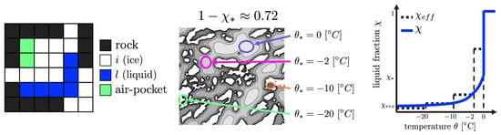
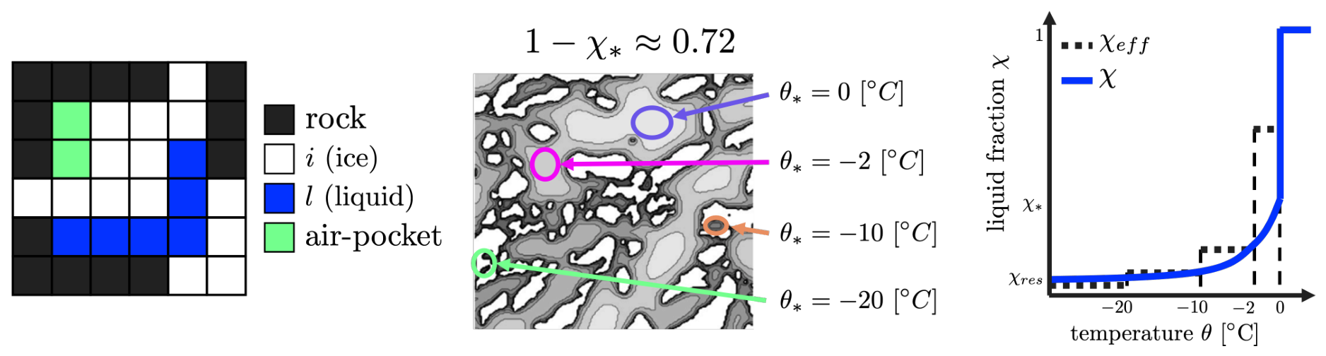
We aim to describe heat conduction in a domain which is composed of rock grains, water in ice and liquid phases, and of air. A typical such domain is depicted in Figure 1.

Figure 1. Illustration of multi-phase nature of soil in permafrost regions and of liquid fraction in such soils depending on the temperature. (Left): cartoon of a small pore-scale region of complex soil which contains rock grains, ice, and liquid and air pockets. (Middle): image from X-ray CT image of permafrost soil from [36]; see also [16], which shows rock grains in white surrounded by water in the pres around the grains. The water pockets feature different freezing temperatures ${\theta }_{*}$ depending on the size of the pores. The volume fraction of the largest pores where ${\theta }_{*}=0$ is $1-{\chi }_{*}$. (Right): the corresponding generalized constitutive law for $\chi$ representing the relationship between $(\theta ,\chi )$ (Figure 3.6, Section 3.3.1, [37]). The ${\chi }_{eff}$ function is piecewise constant, and $\chi$ is a smooth fit.

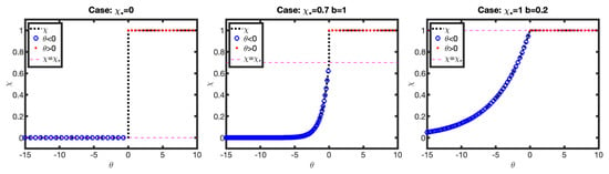
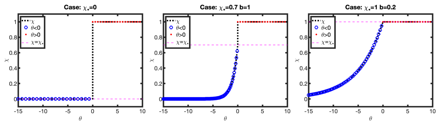
We explain first the constitutive laws for $\mathcal{C}\left(\theta \right)$ and $\mathcal{L}\left(\chi \right)$ in bulk water when the temperature is such that the water can be in the ice phase or in the liquid phase. Typically, the phase change from liquid to ice or ice to liquid occurs at some freezing temperature ${\theta }_{*}$, e.g., ${\theta }_{*}=0{[}^{\circ }\mathrm{C}]$. In bulk water, the liquid fraction $\chi$ equals 1 above the freezing temperature ${\theta }_{*}$, equals 0 below ${\theta }_{*}$, and is in $[0,1]$ at ${\theta }_{*}$. See Figure 2 for illustration of $\chi (·)$.

Figure 2. Illustration of $\chi \in \mathcal{G}[{\theta }_{*},{\chi }_{*},\mathrm{{\rm Y}}]\left(\theta \right)$ for phase change models $\left(ST\right)$ (left) with ${\chi }_{*}=0$, $\left(P^{*}\right)$ when $0<{\chi }_{*}<1$, and $\left(P\right)$ model with ${\chi }_{*}=1$. In $\left(P\right)$ model, the function $\chi (·)$ is continuous.

2.3.1. Generalized Constitutive Law for Liquid Fraction

In soils, the situation is different than in bulk water due to the presence of solid (rock) grains, and the associated microphysics, including the well-known Gibbs phenomenon well-described and analyzed mathematically, e.g., in [10] and reported in the applications literature, e.g., in [38,39,40]. At the temperatures above freezing $\theta >{\theta }_{*}$, all water is in the liquid state, and $\chi =1$. However, when $\theta <{\theta }_{*}$, the soil is only partially frozen, $0\le \chi =\mathrm{{\rm Y}}\left(\theta \right)\le 1$ where $\mathrm{{\rm Y}}(·)$ is some smooth increasing function which describes the fraction of unfrozen water, known as the soil freezing curve; see Figure 2 for an illustration of different generalized constitutive laws for (2).

The properties of $\mathrm{{\rm Y}}$ at ${\theta }_{*}$ are the source of the main difficulty addressed in this paper. In the simplified models considered, e.g., in [11,41], it is assumed that $\mathrm{{\rm Y}}\left({\theta }_{*}\right)=1$ so that $\chi \left(\theta \right)$ is a function continuous at ${\theta }_{*}$. In contrast, in this paper, we allow $\mathrm{{\rm Y}}\left({\theta }_{*}\right)={\chi }_{*}\in [0,1]$; this generalization allows us to use empirical relationships for soils featured in the applications literature. We call this generalized class of models $\left(P^{*}\right)$ and its special cases when ${\chi }_{*}=0$ and $\eta =1$ are called the Stefan problem (the $\left(ST\right)$ model), and when it is the $\left(P\right)$ model, it is ${\chi }_{*}=1$. The framework of $\left(P^{*}\right)$ models unifies the phase-change models considered in [9,10,11,16,41,42] with a single model parameter, denoted as ${\chi }_{*}$, which helps to differentiates between the different classes of models.

2.3.2. Empirical Parametrizations for ($P^{*}$) Model

For the ($P^{*}$) model, we require parametrization by empirically determined parameters. Specifically, we consider a graph $\mathcal{G}$ parametrized by ${\theta }_{*},{\chi }_{*}$ and a function $\mathrm{{\rm Y}}(·)$; these must satisfy some assumptions given below, while ${\theta }_{*},{\chi }_{*},\mathrm{{\rm Y}}(·)$ are specific to and calibrated for the type of soil (sand, silt, clay, etc.). We write

$$\begin{array}{c}\hfill (\theta ,\chi )\in \mathcal{G}[{\theta }_{*},{\chi }_{*},\mathrm{{\rm Y}}],\mathrm{or}\chi \in \mathcal{G}[{\theta }_{*},{\chi }_{*},\mathrm{{\rm Y}}]\left(\theta \right).\end{array}$$

(3)

Here, the symbol “∈” is needed to allow any value of $\chi \in [{\chi }_{*},1]$ at ${\theta }_{*}$, i.e., the multi-valued nature of the relationship at $\theta ={\theta }_{*}$.

We now give concrete examples of constitutive models for $(\theta ,\chi )$ in the ($P^{*}$) model known from the applications literature.

In particular, we consider three empirical models from the applications literature [38,39,40]. We denote these by L, M, or W; the symbols correspond to the primary author’s last name:

$$\begin{array}{ccc}\hfill {\mathrm{{\rm Y}}}^{\left(L\right)}\left(\theta \right)& =& a|{\theta }_{*}{|}^b{(-\theta )}^{-b},\hfill \end{array}$$

(4a)

$$\begin{array}{ccc}\hfill {\mathrm{{\rm Y}}}^{\left(M\right)}\left(\theta \right)& =& {\chi }_{res}+(a-{\chi }_{res})e^{b(\theta -{\theta }_{*})},\hfill \end{array}$$

(4b)

$$\begin{array}{ccc}\hfill {\mathrm{{\rm Y}}}^{\left(W\right)}\left(\theta \right)& =& {\chi }_{res}+a{\left({\displaystyle \frac{b}{b-\theta +{\theta }_{*}}}\right)}^4,\hfill \end{array}$$

(4c)

The models depend on additional empirically fitted parameters such as $a,b,{\chi }_{res}\in [0,1)$ and are given in Table 2. The different choices of $\mathrm{{\rm Y}}$ all satisfy the following Assumption.

Table 2. Data for empirical models for (4) from the applications literature [38,39,40]. The parameter values correspond to clay.

Model	Parameter Values	${\mathit{\chi }}_{*}$	Ref.
$\left(L\right)$	$a=0.3210[-]$, $b=0.271\left[1{/}^{\circ }\mathrm{C}\right]$, ${\theta }_{*}<0{[}^{\circ }\mathrm{C}]$	$0.3210[-]$	[39]
$\left(M\right)$	$a=0.989[-]$, $b=0.16\left[1{/}^{\circ }\mathrm{C}\right]$, ${\chi }_{res}=0.201[-]$	$0.989[-]$	[38]
$\left(W\right)$	$a=0.4[-]$, $b=7.22{[}^{\circ }\mathrm{C}]$, ${\chi }_{res}=0.36[-]$,	$0.76[-]$	[40]

Assumption 1.

Let ${\theta }_{*}\le 0$, ${\chi }_{*}\in [0,1]$, and ${\chi }_{res}\in [0,1)$ be given. Let $\mathrm{{\rm Y}}:{\mathbb{R}}_{-}\to [{\chi }_{res},{\chi }_{*}]$ satisfy the following properties: (i) $\mathrm{{\rm Y}}$ is smooth monotone nondecreasing on ${\mathbb{R}}_{-}$, (ii) ${\lim }_{\theta \to {\theta }_{*}^{-}}\mathrm{{\rm Y}}\left(\theta \right)={\chi }_{*}$, and (iii) ${\lim }_{\theta \to -\infty }\mathrm{{\rm Y}}\left(\theta \right)={\chi }_{res}$. And (iv) if ${\chi }_{*}>0$, then $\mathrm{{\rm Y}}$ must be strictly increasing.

We now define the generalized constitutive law for $(\theta ,\chi )$ in (3) which applies pointwise to $\theta (x,t),\chi (x,t))$ at every $(x,t)$.

Definition 1.

Let Assumption 1 hold. The ($P^{*}$) model is associated with the graph $\mathcal{G}\subset \mathbb{R}\times [0,1]$ parametrized by ${\theta }_{*},{\chi }_{*},\mathrm{{\rm Y}}$

$$\begin{array}{c}\hfill \chi \in \mathcal{G}[{\theta }_{*},{\chi }_{*},\mathrm{{\rm Y}}]\left(\theta \right)=\left\{\begin{array}{cc}1,\hfill & \theta >{\theta }_{*},\hfill \\ [{\chi }_{*},1],\hfill & \theta ={\theta }_{*},\hfill \\ \mathrm{{\rm Y}}\left(\theta \right),\hfill & \theta <{\theta }_{*}.\hfill \end{array}\right.\end{array}$$

(5)

We note that the models L, M, and W were used in [9,10,11,16] in an altered form called “adapted” (or $\left(P\right)$ model) where continuity of $\mathrm{{\rm Y}}$ at ${\theta }_{*}$ was artificially imposed so that ${\chi }_{*}=1$.

We also mention that the Equations (3)–(5) assume instantaneous equilibrium between the temperature $\theta$ and the liquid fraction $\chi$. More general approaches involve, e.g., phase-field models which are analyzed with the use of a Scalar Auxiliary Variable (SAV); see, e.g, [32].

2.4. Heat Capacity Terms

We now describe the constitutive relationship between temperature and energy density $(\theta ,w)$

$$\begin{array}{c}\hfill w\in \alpha [{\theta }_{*},{\chi }_{*},\mathrm{{\rm Y}}]\left(\theta \right)=\mathcal{C}\left(\theta \right)+\mathcal{L}\left(\chi \right);\mathcal{L}\left(\chi \right)=\eta (1-S_g)L\chi ,\end{array}$$

(6)

which involves a heat capacity term $\mathcal{C}\left(\theta \right)$ as well as a latent heat term $\mathcal{L}\left(\chi \right)$, which relies on the relationship $(\theta ,\chi )$ from (3). The term $\mathcal{C}\left(\theta \right)$ describes the heat content of soil, which is a mixture of water, rock, and air, without the phase change. The term $\mathcal{L}\left(\chi \right)$ accounts for phase change. We note that unlike in bulk water, the phase change in partially frozen soils can occur at any temperature $\theta <{\theta }_{*}$, and the amount of latent heat required for that change is proportional to the change in liquid fraction $\chi =\chi \left(\theta \right)$. Figure 3 shows an example of $(\theta ,\chi )$ and $(\theta ,w)$ where $\mathrm{{\rm Y}}(·)$ is from (4).

Figure 3. Illustration of empirical relationship (3) for $(\theta ,\chi )$ (left) and (6) for $(\theta ,w)$ (right). Here, we have used the models $L,M,W$-models.

2.4.1. Regular Portion of Heat Storage Term

Now, we discuss $\mathcal{C}\left(\theta \right)$ in detail. The soil is composed of water, rock, and air materials, with the traditional notion of porosity $\eta$ denoting the volume fraction of fluids and $1-\eta$ of rock. The air phase is assumed to occupy an $S_g$ volume fraction of the fluid space, and $1-S_g$ is occupied by water in liquid or ice phases. We consider ice (i), liquid (l) phases, rock (r), and gas (g) phases. Let $c_p$ denote the heat capacity data for phase p for $p\in \{i,l,r,g\}$. Let the porosity $\eta$ be given and some constant $S_g$ be given. We compute the weighted average of the unfrozen “$uf$” and frozen “$fr$” soil heat capacities defined as

$$\begin{array}{ccc}\hfill c_{uf}& =& (1-\eta )c_r+\eta S_g{c}_g+\eta (1-S_g)c_l,\hfill \end{array}$$

(7a)

$$\begin{array}{ccc}\hfill c_{fr}& =& (1-\eta )c_r+\eta S_g{c}_g+\eta (1-S_g)c_i.\hfill \end{array}$$

(7b)

Given (3), we define the average heat capacity weighted with liquid fraction $\chi \left(\theta \right)$ as

$$\begin{array}{c}\hfill c_{ave}\left(\theta \right)=c_{fr}(1-\chi \left(\theta \right))+c_{uf}\chi \left(\theta \right)=c_{fr}+(c_{uf}-c_{fr})\chi \left(\theta \right).\end{array}$$

We then define the regular portion of energy density as

$$\begin{array}{c}\hfill \mathcal{C}\left(\theta \right)={\int }_{{\theta }_{*}}^{\theta }{c}_{ave}\left(v\right)dv=\left\{\begin{array}{cc}{c}_{uf}(\theta -{\theta }_{*}),\hfill & \theta (x,t)>{\theta }_{*},\hfill \\ (c_{uf}-c_{fr}){\int }_{{\theta }_{*}}^{\theta }\mathrm{{\rm Y}}\left(v\right)dv+c_{fr}(\theta -{\theta }_{*}),\hfill & \theta (x,t)<{\theta }_{*}.\hfill \end{array}\right.\end{array}$$

(8)

Clearly, $\mathcal{C}\left(\theta \right)$ is continuous at $\theta ={\theta }_{*}$ and is the regular portion of $(\theta ,w)$.

2.4.2. Multi-Valued Portion of Heat Storage

The portion $\mathcal{L}\left(\chi \right)$ accounts for the thawing/freezing of the water fraction $\eta (1-S_g)$ of soil volume at any temperature at or below ${\theta }_{*}$, with the rate of change measured by the liquid fraction $\mathrm{{\rm Y}}\left(\theta \right)$ and latent heat L. For $\theta >{\theta }_{*}$, all water is thawed, and we have $\mathcal{L}\left(1\right)=\eta L(1-S_g)$. At $\theta ={\theta }_{*}$, any change depends on the current value of $\chi \in [{\chi }_{*},1]$. The definition of $\mathcal{L}\left(\chi \right)$ is summarized in

$$\begin{array}{c}\hfill (\theta ,\chi )\in \mathcal{G};\mathcal{L}\left(\chi \right)=\left\{\begin{array}{cc}\eta (1-S_g)L,\hfill & \theta >{\theta }_{*},\hfill \\ \eta (1-S_g)L\chi ,\hfill & \chi \in [{\chi }_{*},1],\theta ={\theta }_{*},\hfill \\ \eta (1-S_g)L\mathrm{{\rm Y}}\left(\theta \right),\hfill & \theta <{\theta }_{*},\hfill \end{array}\right.\end{array}$$

2.4.3. Summary of Heat Storage

In summary, we construct (6) as a sum of $\mathcal{C}\left(\theta \right)$ and $\mathcal{L}\left(\chi \right)$ with $\chi \in \mathcal{G}\left(\theta \right)$, and from there we have

$$\begin{array}{c}\hfill w\left(\theta \right)\in \alpha \left(\theta \right)=\left\{\begin{array}{cc}{w}_{+}\left(\theta \right),\hfill & \theta >{\theta }_{*},\hfill \\ \eta (1-S_g)L[{\chi }_{*},1],\hfill & \theta ={\theta }_{*},\hfill \\ w_{-}\left(\theta \right),\hfill & \theta <{\theta }_{*},\hfill \end{array}\right.\end{array}$$

(9a)

where

$$\begin{array}{ccc}\hfill w_{+}\left(\theta \right)& =& c_{uf}(\theta -{\theta }_{*})+\eta (1-S_g)L,\hfill \end{array}$$

(9b)

$$\begin{array}{ccc}\hfill w_{-}\left(\theta \right)& =& c_{fr}(\theta -{\theta }_{*})+(c_{uf}-c_{fr}){\int }_{{\theta }_{*}}^{\theta }\mathrm{{\rm Y}}\left(v\right)dv+\eta (1-S_g)L\mathrm{{\rm Y}}\left(\theta \right).\hfill \end{array}$$

(9c)

We see that $w_{+}(·)$ is an affine function of $\theta$, but $w_{-}(·)$ is given by a complicated algebraic formula. We give useful auxiliary calculations of the integrals involved in Table A1. See Figure 3 for illustration.

2.4.4. Inverse Relationship for $(\theta ,\chi ,w)$

In a computational model, we shall require the values of all the variables $\theta (x,t)$, $\chi (x,t)$, $w(x,t)$ at any point $(x,t)\in \mathcal{Q}$ (or on a grid covering $\mathcal{Q}$). It is important to emphasize how they are coupled together so we can define the inversion formulas.

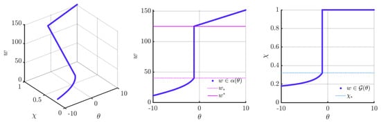
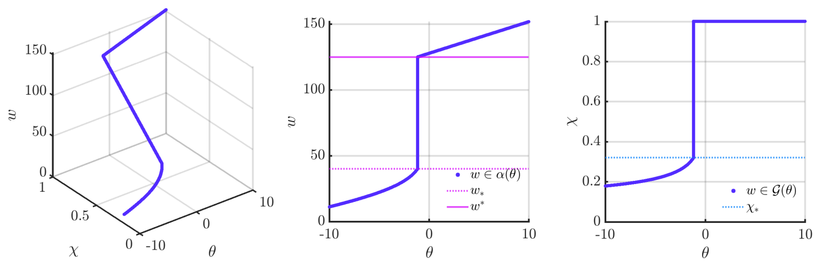
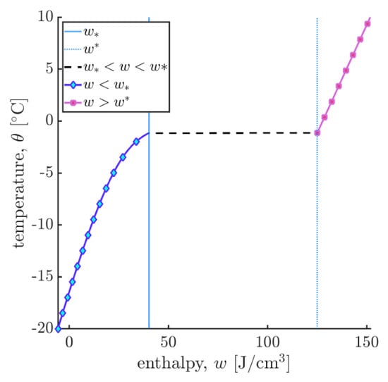
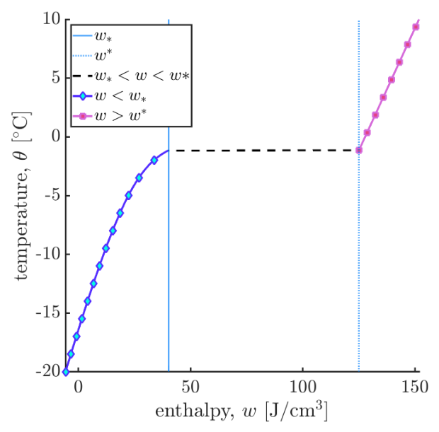
The generalized constitutive laws for $(\theta ,\chi )$ in (5) and $(\theta ,w)$ in (9) are given with multi-valued graphs for mathematical clarity. However, under Assumption 1, $w_{-}$ and $w_{+}$ are monotone increasing, and the physical meaning is clear and unambiguous for the collection of unknowns $(\theta ,\chi ,w)$ together, following from the thermodynamics principles. The relationships between $(\theta ,\chi ,w)$ are multi-valued when projected on the $(\theta ,w)$ and $(\theta ,\chi )$ planes. This is illustrated in Figure 4.

Figure 4. Illustration of the multi-valued graphs and the relationships (5) and (9). (Left): plot $(\theta ,\chi ,w)\subset {\mathbb{R}}^3$ when $(\theta ,\chi )\in \mathcal{G}$, $(\theta ,w)\in \alpha$. Its projections on $(\theta ,w)$ plane (middle) and on in $(\theta ,\chi )$ plane (right) appear multivalued, but the full relationship $(\theta ,\chi )\leftrightarrow w$ is bijective whenever $(\theta ,\chi )\in \mathcal{G}$.

We clarify now the inversion formulas. Define the auxiliary symbols

$$\begin{array}{c}\hfill w_{*}=\underset{\theta \to {\theta }_{*}^{-}}{\lim }{w}_{-}\left(\theta \right)=\eta (1-S_g)L{\chi }_{*},\mathrm{and}{w}^{*}=\underset{\theta \to {\theta }_{*}^{+}}{\lim }{w}_{+}\left(\theta \right)=\eta (1-S_g)L.\end{array}$$

(10)

When $\theta >{\theta }_{*}$, $w>w^{*}$ is determined uniquely from $\theta$, and $\theta$ can be found uniquely from $w>w_{*}$; this is easy since $w_{+}(·)$ is affine. When $\theta ={\theta }_{*}$, $w_{*}\le w\le w^{*}$, and w depends affinely on $\chi$; $\chi$ can be determined uniquely from w. In turn, when $\theta <{\theta }_{*}$, $w<w_{*}$, and w is determined uniquely from $\theta$; as well $\theta$ can be found uniquely from $w<w_{*}$ since $w_{-}$ is monotone increasing. In other words, together, $(\theta ,\chi )$ are given by a bijection

$$\begin{array}{c}\hfill \psi \left(w\right)=(\theta ,\chi ).\end{array}$$

(11)

We refer to Figure 5 for an illustration of $\psi (·)$.

Figure 5. Illustration of $\psi \left(w\right)=(\theta ,\chi )$ from (12) with L-model (4a). We see that when $w<w_{*}$ or $w>w^{*}$, the relationship $(w,\theta )$ is invertible. Also, we see that between $w_{*}$ and $w^{*}$, the relationship $(w,\theta )$ is not invertible. However, for $w\in (w_{*},w^{*})$, one can find a unique $\chi$ so that $(w,\chi )$ is invertible (plot not shown). In summary, we write that $w\leftrightarrow (\theta ,\chi )$ is a bijection for $\chi \in \mathcal{G}\left(\theta \right)$.

Remark 1.

Let Assumption 1 hold, $S_g\in (0,1),\eta \in (0,1)$ be given, and $w_{*}$ and $w^{*}$ be given by (10). Then, we have $\psi \left(w\right)=(\theta ,\chi )$

$$\begin{array}{c}\hfill \psi \left(w\right)=\left\{\begin{array}{ccc}\mathit{when}w<w_{*}:\hfill & \mathit{find}\theta :w_{-}\left(\theta \right)=w,\hfill & \mathit{calculate}\chi =\mathrm{{\rm Y}}\left(\theta \right),\hfill \\ \mathit{when}w\in [w_{*},w^{*}]:\hfill & \theta ={\theta }_{*},\hfill & \chi =w/w^{*},\hfill \\ \mathit{when}w>w^{*}:\hfill & \mathit{calculate}\theta ={\theta }_{*}+(w-w^{*})/c_{uf},\hfill & \chi =1,\hfill \end{array}\right.\end{array}$$

(12)

where $w_{-}(·)$ is given in (9c). However, there is a complication, since $w_{-}\left(\theta \right)$ does not have an explicit algebraic formula for its inverse. We shall therefore require a numerical inversion formula $\theta =w_{-}^{-1}\left(w\right)$ to solve

$$\begin{array}{c}\hfill w_{-}\left(\theta \right)-w=0,\end{array}$$

(13)

We discuss numerical inversion formulas (called local solvers) in Section 5, and we apply these to (13) in Section 6.1.

2.5. Thermal Conductivity

In soil, thermal conductivity must be considered a phase-weighted average of the thermal conductivities of the materials and phases present. While most accurate values of such properties can be found by homogenization [16], we shall consider here geometric averages, which are widely used in the literature [9,10,38,43]; see also [10] for a comparison.

Let $k_p$ denote the thermal conductivity data for phase p for $p\in \{i,l,r,g\}$. With the phase fractions known, we define the thermal conductivity by

$$\begin{array}{ccc}\hfill k\left(\theta \right)& =& k_r^{(1-\eta )}{k}_l^{\eta (1-S_g)\chi \left(\theta \right)}{k}_i^{\eta (1-S_g)(1-\chi \left(\theta \right))}{k}_g^{\eta S_g}.\hfill \end{array}$$

(14)

2.6. Model Summary

The model ($P^{*}$) is now fully given by (2) complemented by the definitions (5), (9) and (14). It is a nonlinear parabolic PDE.

Remark 2.

We do not address the well-posedness of the $\left(P^{*}\right)$ model problem here; rather, we refer to the literature [9,44,45,46,47] for the well-posedness of similar problems posed in the sense of distributions that may be extended to fit to $\left(P^{*}\right)$; see also (Chapter 5, [37]) for details of this formulation for the ($P^{*}$) model. In particular, the model (ST), which is a special case of ($P^{*}$) is well known to not have classical solutions and only to have low regularity solutions in the sense of distributions; we refer to [45,47] for details.

3. Discretization

In this Section, we define the approximation of the solutions $(\theta ,w,q)$ to (2), aiming to (i) respect the low regularity of the solutions as well as (ii) maintain the conservation principles, while (iii) maintaining efficiency and ease of implementation. In particular, we choose the discretization based on the Mixed Finite Element method on a rectangular grid, which is known to satisfy these properties, as is well explained in [48]. This discretization can be also interpreted as cell-centered finite differences (CCFD), or the lowest-order finite volume method.

To satisfy (i), we approximate the temperature $\theta$ and enthalpy w using the lowest-order piecewise constants referred to as P0 finite elements. With these, (6) is implemented pointwise. For (ii), we approximate the heat flux q (2b) with RT_[0] elements. Regarding (iii), the scheme we implement can be implemented very efficiently in any spatial domain in any dimension. We only describe the notation for $l=1$ and refer to [9,10,11] for $l>1$.

3.1. Spatial and Temporal Discretization

Assume that the rectangular grid ${\mathcal{T}}^h$ of $N_{\omega }$ elements ${\left({\omega }_j\right)}_j$ covers $\mathrm{\Omega }\subset \mathbb{R}$ such that $\overline{\mathrm{\Omega }}={{\displaystyle \overline{\bigcup }}}_j{\omega }_j$ with $h={\max }_j\left|{\omega }_j\right|$ for $j=1,\dots ,N_{\omega }$. Each element ${\omega }_j$ has a cell center denoted by $x_j$ and cell edges denoted with $x_{j\pm 1/2}$. We consider the finite element space $M_h\subset L^2\left(\mathrm{\Omega }\right)$ of piecewise constants on ${\mathcal{T}}_h$, where we approximate scalar quantities such as $w,\theta ,\chi$, and $X_h\subset H_{div}\left(\mathrm{\Omega }\right)$ serves as the lowest-order Raviart–Thomas space on ${\mathcal{T}}^h$, where we approximate the fluxes q.

We also set up temporal discretization, with time step $\tau$. For simplicity, we consider a uniform temporal grid such that with $t_0=0$,

$$\begin{array}{c}\hfill t_n=t_{n-1}+\tau ,n=1,\dots N.\end{array}$$

(15)

The approximation to (2) closely follows the formulation from [48], more recently defined for nonlinear heat equation in [9,11]. We seek the approximations ${\theta }_h\in M_h,w_h\in M_h,{\chi }_h\in M_h$, each identified with its vectors of degrees of freedom, respectively, $\mathrm{\Theta },W,\mathcal{X}$. For time discrete values at $t=t_n$, we seek vectors ${\mathrm{\Theta }}^n,W^n,{\mathcal{X}}^n$. For example, ${\mathrm{\Theta }}_j^n={\theta }_h^n{|}_{{\omega }_j}$.

We also denote by $Q^n$ the vector of degrees of freedom of $q_h^n$ in their respective basis at $t=t_n$, and we identify the flux with its values on the cell edges such that $Q_{j\pm 1/2}^n=q_h^n{|}_{x_{j\pm 1/2}}$.

Assume that $w_h^0\in M_h$ is given. The fully discrete mixed weak formulation of (2) is as follows: given $w_h^{n-1}\in M_h$, we seek $({\theta }_h^n,q_h^n)\in M_h\times X_h$ such that

$$\begin{array}{ccc}\hfill ({\displaystyle \frac{w_h^n-w_h^{n-1}}{\tau }},{\eta }_h)+(\nabla ·q_h^n,{\eta }_h)& =& (f^n,{\eta }_h),\forall {\eta }_h\in M_h,\hfill \end{array}$$

(16a)

$$\begin{array}{ccc}\hfill {({\tilde{k}}^{-1}{q}_h^n,{\psi }_h)}_h-({\theta }_h^n,\nabla ·{\psi }_h)& =& -{({\theta }_D,{\psi }_h·\nu )}_{\partial \mathcal{Q}},\forall {\psi }_h\in X_h,\hfill \end{array}$$

(16b)

$$\begin{array}{c}\hfill w_h^n\in \alpha \left({\theta }_h^n\right)\equiv w_j^n\in \alpha \left({\theta }_j^n\right),\end{array}$$

(16c)

$$\begin{array}{c}\hfill {\chi }_h^n\in \mathcal{G}\left({\theta }_h^n\right)\equiv {\chi }_j^n\in \mathcal{G}\left({\theta }_j^n\right).\end{array}$$

(16d)

The last equations enforce the phase behavior (9) at every degree of freedom j. We omitted the parametrization of $\alpha =\alpha ({\theta }_{*},{\chi }_{*},\mathrm{{\rm Y}})$ and of $\mathcal{G}=\mathcal{G}({\theta }_{*},{\chi }_{*},\mathrm{{\rm Y}})$ for simplicity. Also, $\tilde{k}\in M_h$ is an approximation to $k\left({\theta }_h^n\right)$, which helps to eliminate the flux unknowns, as explained below.

Let ${\mathbf{1}}_{{\omega }_j}$ be the characteristic function of the element ${\omega }_j$ and $\mathcal{V}$ be the diagonal matrix of cell volumes with ${\mathcal{V}}_{jj}=h_j$ for all $j=1,\dots ,N_{\omega }$ so that $({\psi }_h,{\xi }_h)={\left(\mathrm{\Psi }\right)}^T\mathcal{V}\Xi$ for any ${\psi }_h,{\xi }_h\in M_h$. We define the vector $F^n$ by $F_j^n=(f,{\mathbf{1}}_{{\omega }_j})$.

We recall a well-known numerical integration technique from [49] to approximate $(k^{-1}{q}_h^n,{\psi }_j)$ with a trapezoidal rule by ${(k^{-1}{q}_h^n,{\psi }_j)}_h$, as in in (16b). This technique leads to a lumped single system of equations rather than a saddle system. We define $\tilde{k}\in M_h$

$$\begin{array}{c}\hfill \tilde{k}{{|}_{{\omega }_j}={\left(k\left({\theta }_h^n\right)\right|}_{{\omega }_j})}^{-1}.\end{array}$$

(17)

Then, ${(k^{-1}{q}_h^n,{\psi }_j)}_h$ involves a single scaling constant ${\mathcal{T}}_{j+1/2}^n$ called transmissibility,

$$\begin{array}{ccc}\hfill {\mathcal{T}}_{j+1/2}^n=2{(h_j{\tilde{k}}_j+h_{j+1}{\tilde{k}}_{j+1})}^{-1},& & j=1,\dots ,N_{\omega }-1,\hfill \end{array}$$

(18a)

with the transmissibilities on the Dirichlet portion of the boundary given as

$$\begin{array}{ccc}\hfill {\mathcal{T}}_{1/2}^n=2{\left(h_1{\tilde{k}}_1\right)}^{-1},& & {\mathcal{T}}_{N_{\omega }+1/2}^n=2{\left(h_{N_{\omega }}{\tilde{k}}_{N_{\omega }}\right)}^{-1}.\hfill \end{array}$$

(18b)

We refer to recent work in [9,11] for the specifics and examples in $l=1$ and $l=2$.

Next, we let ${\mathcal{B}}^T$ be the matrix defined so that $-({\theta }_h^n,\nabla ·{\psi }_h)={\mathcal{B}}^T{\mathrm{\Theta }}^n$. Similarly, we obtain $(\nabla ·q_h^n,{\eta }_h)=-\mathcal{B}{Q}^n$. We can now write the matrix vector form of (16)

$$\begin{array}{c}\hfill {\displaystyle \frac{1}{\tau }}\mathcal{V}{W}^n-\mathcal{B}{Q}^n=F^n+{\displaystyle \frac{1}{\tau }}\mathcal{V}{W}^{n-1},\end{array}$$

(19a)

$$\begin{array}{c}\hfill \tilde{K}{Q}^n+{\mathcal{B}}^T{\mathrm{\Theta }}^n={\mathcal{B}}^T{\mathrm{\Theta }}_D^n,\end{array}$$

(19b)

$$\begin{array}{c}\hfill W_j^n\in \alpha [{\theta }_{*},{\chi }_{*},\mathrm{{\rm Y}}]\left({\mathrm{\Theta }}_j^n\right),\end{array}$$

(19c)

$$\begin{array}{c}\hfill ({\mathrm{\Theta }}_j^n,{\mathcal{X}}_j^n)\in \mathcal{G}[{\theta }_{*},{\chi }_{*},\mathrm{{\rm Y}}].\end{array}$$

(19d)

Here, the diagonal matrix $\tilde{K}$ collects the (inverses of) (positive) nonlinear transmissibilities in (18) and is thus nonsingular, but its entries depend on ${\mathrm{\Theta }}^n$ due to (17). We now define

$$\begin{array}{c}\hfill \mathcal{A}=\mathcal{B}{\tilde{\mathcal{K}}}^{-1}{\mathcal{B}}^T,\end{array}$$

(20)

which depends on ${\mathrm{\Theta }}^n$, and we eliminate $Q^n$ in (19), obtaining from (19a) and (19b) the system

$$\begin{array}{c}\hfill \mathcal{V}{W}^n+\tau \mathcal{A}{\mathrm{\Theta }}^n=\tau F^n+\mathcal{V}{W}^{n-1}+\tau \mathcal{A}{\mathrm{\Theta }}_D^n,\end{array}$$

(21a)

This system is supplemented with the pointwise relationships (19c), with (19d) needed to evaluate $\alpha (·)$ pointwise. We rewrite these here for convenience as

$$\begin{array}{c}\hfill W_j^n\in \alpha \left({\mathrm{\Theta }}_j^n\right);({\mathrm{\Theta }}_k^n,{\mathcal{X}}_j^n)\in \mathcal{G}.\end{array}$$

(21b)

3.2. Algebraic System and Primary Unknowns

We see that (21a) is a nonlinear algebraic system of equations in two unknowns—$W^n$ and ${\mathrm{\Theta }}^n$. On the left-hand side, we have a linear expression in $W^n$ and a nonlinear expression in ${\mathrm{\Theta }}^n$ coupled pointwise by (21b).

A nonlinear solver to solve (21) proceeds by iteration with respect to a primary unknown. We choose $W^n$ as the primary unknown: we start with an initial guess $W^{n,\left(0\right)}$ and iterate $W^{n,(k-1)}\to W^{n,\left(k\right)}$, with $k=1,\dots$ until convergence.

We apply an iterative solver to (21a) which we call global, because it works simultaneously on all components of the vector guess $W^{n,\left(k\right)}$. At any guess $W^{n,\left(k\right)}$, we must evaluate all portions of the equation (21a). In particular, we evaluate ${\mathrm{\Theta }}^{n,\left(k\right)}$, i.e., we must invert (21b) pointwise at every j; we call the required solver local. As explained in Remark 1, the inversion is complicated due to the form of $\alpha (·)$ and in particular due to the properties of $w_{-}(·)$ in (9c).

Remark 3.

In this paper, we use W as the primary unknown, which is the only option for ($P^{*}$) model, but this choice requires a local solver. For models which are simpler than ($P^{*}$), such as the (P) model, one can use Θ as a primary unknown, and no local solver is needed, but the global solver is less robust than with W as the primary unknown [9,11].

In Section 4, we identify the specific global and local solvers. These are applied in Section 5 to (21). Finally, we note that $\mathcal{A}$ depends on ${\mathrm{\Theta }}^n$; we discuss how to handle this in Section 5.3.

4. Solvers

In this Section, we define algorithms to solve a general nonlinear problem

$$\begin{array}{ccc}\hfill g\left(x\right)=0,& & x\in V\subset {\mathbb{R}}^l.\hfill \end{array}$$

(22)

for a continuous function $g(·):{\mathbb{R}}^l\to {\mathbb{R}}^l$.

Our algorithm to find the root x of (22) is developed by iteration. We start with an initial guess $x^{\left(0\right)}$ and define subsequent iterates

$$\begin{array}{c}\hfill x^{\left(k\right)}\to x^{(k+1)},k=0,1,2\dots \end{array}$$

(23)

We iterate until the following stopping criterium holds.

Definition 2.

(Stopping Criterium) Let $k^{max}\ge 1,{\tau }_a>0,{\tau }_r>0$ (maximum number of iterations, absolute and relative tolerance) be given and select some norm $\Vert ·\Vert$ on ${\mathbb{R}}^l$. The iteration (23) stops in one of the following circumstances: (i) when $k>k^{max}$ or when $k\le k^{max}$ and (ii) when the absolute residual criterium holds: $\Vert g\left(x^{\left(k\right)}\right)\Vert <{\tau }_a$ or (iii) when the relative tolerance criterium holds $\Vert g\left(x^{(k-1)}\right)\Vert <{\tau }_r\Vert g\left(x^{\left(0\right)}\right)\Vert$.

As explained in Section 3.2, we need two types of nonlinear solvers: global solvers when $l>1$ and $g(·)$ is piecewise smooth only. We also require local solvers when $l=1$, and $g(·)$ is convex on some interval V. In Section 4.1 and Section 4.2, we make precise the algorithms we found most promising for these two contexts, respectively.

The algorithms we define are based on well-known classical methods, including Newton’s methods, its variants, and its Anderson accelerated versions, which all exploit the Fréchet derivative $Dg(·)$ of $g(·)$ or its approximations. The Newton-based algorithms are proven in [17] to converge only under strong assumptions called “standard assumptions”, including the $C^1$ smoothness of $g(·)$, Lipschitz continuity of $Dg$ and boundedness of the inverse of $Dg$. If these hold, the algorithms converge q-quadratically [17] or q-superlinearly depending on the algorithm. We also mention related work on Anderson acceleration methods for fixed point problems; for these, the analysis is established for smooth problems in e.g., [23], while the analysis for the semi-smooth case is emerging; see, e.g., recent work in [50,51,52]. At the same time, while numerical evidence is very promising, the analysis of Newton–Anderson algorithms for smooth problems is still emerging; see [22,24].

However, the relationships we consider in this paper are multi-valued at the phase transition temperature, and the resulting nonlinear functions $g(·)$ are only semi-smooth. In fact, we will only assume that the solution to (22) exists and that $g(·)$ is continuous and semi-smooth near the root. This notion and appropriate algorithms are discussed in Section 4.1.3.

When $l=1$, we also consider solvers which exploit the use of bracketing of the solution, i.e., the subsequent iterates $x^{\left(k\right)}$ need to belong to some interval $V\subset R$ for all k.

In the rest of this Section, we define the algorithms. In subsequent sections, we apply them to the specific ($P^{*}$) problem and evaluate the performance of the algorithms. In the end, the algorithms show promise judging by the numerical evidence. Motivated by this initial success, we aim to conduct analysis of their convergence, and in particular consider Newton–Anderson in the semi-smooth case, but this analysis is, however, outside our present scope.

4.1. Global Solvers

In this section, we recall classical algorithms based on the Newton–Raphson method and define their accelerated versions as well as their semi-smooth versions. We refer to [17] for the background information and details.

Specifically, the classical Newton’s algorithm uses the (Fréchet) derivative $Dg$ of g, which is the matrix of partial derivatives of $g(·)$. Alternatively, one can use some approximations to $Dg$, e.g., as in a secant method. We recall first the Newton–Raphson algorithm, then its accelerated version called the Newton–Anderson acceleration [22], which are both defined for smooth functions.

Next, when $g(·)$ is only piecewise smooth, the algorithms use some selection from the subdifferential $\partial g$ of g, also called the Clarke generalized Jacobian (or derivative). We define these as well as the semi-smooth Newton method, which chooses a particular choice of Jacobian from the subdifferential; here, we follow [25].

Finally, we develop a new concept of semismooth Newton–Anderson iteration and show an example. For each algorithm, we state the regularity assumptions on the data.

4.1.1. Newton–Raphson Method

Let $g:V\subset {\mathbb{R}}^l\to {\mathbb{R}}^l$ be continuously Frećhet differentiable for which we want to solve (22). Denote $J_g=Dg$, and assume $J_g\in {\mathbb{R}}^{l\times l}$ is Lipschitz continuous and nonsingular on ${\mathbb{R}}^l$. Assume also that $x^{\left(0\right)}$ is sufficiently close to the root x of (22). For other details of the so-called “standard assumptions”, see (Assumption 4.3.1, [17]).

It is well known that iterations similar to Algorithm 1 when $J_g$ is not exact but rather uses some approximation $J_g\approx Dg$ may also converge under appropriate assumptions. For example, $J_g$ can be calculated as a finite difference approximation or when one takes in k-th step $J_g=Dg\left(x^{\left(k^{*}\right)}\right)$, where $k^{*}$ is some chosen fixed iteration step.

Algorithm 1

(Newton–Raphson iteration). For $k=1,2,\dots$, execute the steps as follows

1.

In each step k, evaluate $g\left(x^{(k-1)}\right)$ and check (Stopping Criterium). If it holds, stop.

2.

If no, evaluate the Jacobian $J_g=Dg\left(x^{(k-1)}\right)$.

3.

Find $\delta x^{\left(k\right)}$ as the solution to the linear system

$$\begin{array}{c}\hfill J_g\delta x^{\left(k\right)}=-g\left(x^{(k-1)}\right).\end{array}$$

(24a)

4.

Calculate the updated guess

$$\begin{array}{c}\hfill x^{\left(k\right)}=x^{(k-1)}+\delta x^{(k-1)}.\end{array}$$

(24b)

5.

Set $k\to k+1$ and go back to step (1).

These modified algorithms may require fewer evaluations of $Dg$ per iteration, but they typically require more iterations to converge than those with an exact Jacobian. See, e.g., Section 4.2.2.

4.1.2. Newton–Anderson Method

This method [22,53] is an iterative extrapolation method which takes into account the m of the previous Newton corrections $\delta x^{\left(k\right)}$ and of the update steps $x^{\left(k\right)}$, where m refers to the depth size of the method.

Assume that $g(·)$ is continuously Fréchet differentiable with a well-defined $Dg$ which is Lipschitz continuous and with a bounded inverse (Assumption 1, Lemma 1, [22]). Then, if the initial guess is close enough to the root, the iteration converges at least q-super-linearly. For degenerate and nondegenerate problems, the method has been observed to have a subquadratic order of convergence (Section 4, [22]).

The steps below take advantage of those from Algorithm 1.

Algorithm 2

(Newton–Anderson with depth $m>1$). Set a depth size of $m\ge 1$, and choose an initial guess $x^{\left(0\right)}$. Compute the first Newton update $x^{\left(1\right)}=x^{\left(0\right)}+\delta x^{\left(1\right)}$ with (24a).

• Iterate $k\ge 1$ until (Stopping Criterium) holds.

1.

Set $m_k=\min \{k,m\}$.

2.

Find $\delta x^{\left(k\right)}$as the solution to (24a).

3.

Construct the matrix of previous residuals ${\Delta }_{\delta x}^{\left(k\right)}$ where the jth column is given by

$$\begin{array}{ccc}\hfill {\left({\Delta }_{\delta x}^{\left(k\right)}\right)}_j=\delta x^{(m_k+1-j)}-\delta x^{(m_k-j)},& & j=1,\dots ,m_k.\hfill \end{array}$$

(25a)

4.

Construct the matrix of previous updates ${\Delta }_x^{\left(k\right)}$ where the jth column is given by

$$\begin{array}{ccc}\hfill {\left({\Delta }_x^{\left(k\right)}\right)}_j=x^{(m_k-j)}-x^{(m_k-1-j)},& & j=1,\dots ,m_k.\hfill \end{array}$$

(25b)

5.

Compute ${\gamma }^{\left(k\right)}={\mathrm{argmin}}_{\gamma \in {\mathbb{R}}^{m_k}}\Vert \delta x^{\left(k\right)}-{\Delta }_{\delta x}^{\left(k\right)}\gamma \Vert$. In general, we use least squares.

6.

Evaluate Newton–Anderson update step $x^{(k+1)}$:

$$\begin{array}{c}\hfill x^{(k+1)}=x^{\left(k\right)}+\delta x^{\left(k\right)}-\left({\Delta }_x^{\left(k\right)}+{\Delta }_{\delta x}^{\left(k\right)}\right){\gamma }^{\left(k\right)}.\end{array}$$

(25c)

Remark 4.

We note that for large m and l, Step 5 might be expensive. We also remark that when $m=0$, the algorithm is the same as Algorithm 1.

4.1.3. Semi-Smooth Newton Methods

We aim now to relax the smoothness assumptions in Section 4.1.1 and Section 4.1.2 and only require $g(·)$ to be only (locally) Lipschitz continuous on V rather than $C^1$ smooth. In the algorithms, we shall use a selection from the generalized (Clarke) derivative, a set valued map, which we now define.

We follow [25] and paraphrase the necessary definitions involved. First, we recall that for set S, the convex hull $\mathrm{co}\left\{S\right\}$ of S is the smallest convex set containing S. Also, we let $S_g\subset V$ denote the set of all points $x\in V$ such that g admits a Fréchet derivative $Dg\left(x\right)$.

Definition 3

(Clarke’s generalized Jacobian and semi-smooth functions (pp. 10, 25, [25])). We define the set-valued Bouligand derivative ${\partial }_{B}g:{\mathbb{R}}^l\to {\mathbb{R}}^{l\times l}$

$$\begin{array}{c}\hfill {\partial }_{B}g\left(x\right)=\{A\in {\mathbb{R}}^{l\times l}:\exists x_k\in S_g:x_k\to x,Dg\left(x_k\right)\to A\},\end{array}$$

(26)

and its convex hull, the Clarke generalized Jacobian

$$\begin{array}{c}\hfill \partial g\left(x\right)=\mathrm{co}\left({\partial }_{B}g\left(x\right)\right).\end{array}$$

(27)

The function $g(·)$ is called semi-smooth if $g(·)$ is Gâteaux differentiable at x, and if

$$\begin{array}{c}\hfill \underset{M\in \partial g(x+h)}{\sup }\parallel g(x+h)-g\left(x\right)-Mh\parallel =\mathcal{O}(\parallel h\parallel ),\mathrm{as}h\to 0.\end{array}$$

(28)

To solve (22) when $g(·)$ is semi-smooth, we only need to identify which elements from the set $\partial g\left(x\right)$ we need to select. We follow (Algorithm 2.11, [25]).

Algorithm 3

(Semi-smooth Newton’s method). For $k=1,2,\dots$

1.

Evaluate $g\left(x^{\left(k\right)}\right)$ and check (Stopping Criterium). If satisfied, stop.

2.

Otherwise, choose some nonsingular $M_k\in \partial g\left(x^{\left(k\right)}\right)$.

3.

Find $s^{\left(k\right)}$ by solving $M_k{s}^{\left(k\right)}=-g\left(x^{\left(k\right)}\right)$, and set $x^{(k+1)}=x^{\left(k\right)}+s^{\left(k\right)}$.

4.

Go back to (1).

Proposition 2.12 from [25] guarantees that if all $M_k$ from Step 2 of the algorithm are nonsingular, and if (28) holds, then the Algorithm 3 converges q-superlinearly to the root of (22).

4.1.4. Semi-Smooth Newton–Anderson Method, Depth Size $m=1$

Now, we combine methods from Section 4.1.2 and Section 4.1.3. Let $g:V\subset {\mathbb{R}}^l$ be semi-smooth such that for any $M\in \partial g$, M is nonsingular.

Algorithm 4

(Semi-smooth Newton–Anderson method, depth $m=1$). Let $x^{\left(0\right)}\in V$ be given. Choose $M_0\in \partial g\left(x^{\left(0\right)}\right)$ and find $x^{\left(1\right)}=x^{\left(0\right)}-M_0^{-1}g\left(x^0\right)$. For $k=1,2,\dots$

1.

Compute $g\left(x^{\left(k\right)}\right)$ and check (Stopping Criterium). If satisfied, stop.

2.

Otherwise, choose some $M_k\in \partial g\left(x^{\left(k\right)}\right)$.

3.

Find $s^{\left(k\right)}$ from solving $M_k{s}^{\left(k\right)}=-g\left(x^{\left(k\right)}\right)$.

4.

Compute the Newton–Anderson optimization parameter ${\gamma }^{\left(k\right)}\in \mathbb{R}$

$$\begin{array}{c}\hfill {\gamma }^{\left(k\right)}={\displaystyle \frac{⟨s^{\left(k\right)},s^{\left(k\right)}-s^{(k-1)}⟩}{\Vert s^{\left(k\right)}-s^{(k-1)}{\Vert }^2}}.\end{array}$$

(29)

5.

Evaluate the Newton–Anderson update step $x^{(k+1)}$

$$\begin{array}{c}\hfill x^{(k+1)}=x^{\left(k\right)}+s^{\left(k\right)}-{\gamma }^{\left(k\right)}\left(x^{\left(k\right)}-x^{(k-1)}+(s^{\left(k\right)}-s^{(k-1)})\right).\end{array}$$

(30)

6.

Go back to (1).

This algorithm is easily extended to $m>1$.

Algorithm 5

(Semi-smooth Newton–Anderson method, depth $m\ge 1$). Extend Algorithm 4 with steps 3–6 of Algorithm 2.

To our knowledge, this statement of the Algorithm 4 is new. Its analysis is not available but is subject of our future work.

4.1.5. Example

We illustrate the theoretical concepts and the algorithms in the semi-smooth setting of Algorithms 3 and 4 when $l=1$.

Example 1.

We consider

$$\begin{array}{c}\hfill g\left(x\right)=\max (x^2,x^3)-0.5=\left\{\begin{array}{cc}{x}^2-0.5,\hfill & x\le 1,\hfill \\ x^3-0.5,\hfill & x>1.\hfill \end{array}\right.\end{array}$$

(31)

Here, $g(·)$ is semismooth, and $x^{(*)}=1/\sqrt{2}$ is the solution to (22) in $V=(0,\infty )$.

We first construct the B-subdifferential and the corresponding Clarke’s generalized Jacobian for $g\left(x\right)$

$$\begin{array}{ccc}\hfill {\partial }_{B}g\left(x\right)=\left\{\begin{array}{cc}\left\{2x\right\},\hfill & x<1,\hfill \\ \{2,3\},\hfill & x=1,\hfill \\ \left\{3x^2\right\},\hfill & x>1,\hfill \end{array}\right.& & \partial g\left(x\right)=\left\{\begin{array}{cc}\left\{2x\right\},\hfill & x<1,\hfill \\ [2,3],\hfill & x=1,\hfill \\ \left\{3x^2\right\},\hfill & x>1.\hfill \end{array}\right.\hfill \end{array}$$

(32)

For implementation of the semi-smooth Newton and Newton–Anderson method, we select the following $M\left(x\right)\in \partial g\left(x\right)$, which is nonsingular on V

$$\begin{array}{c}\hfill M\left(x\right)=\left\{\begin{array}{cc}2x,\hfill & x<1,\hfill \\ \frac{5}{2},\hfill & x=1,\hfill \\ 3x^2,\hfill & x>1.\hfill \end{array}\right.\end{array}$$

(33)

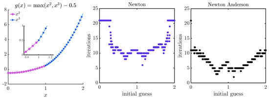
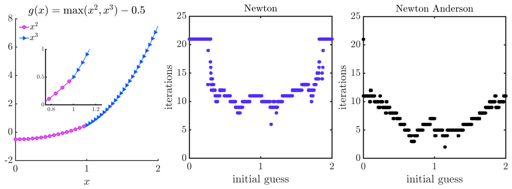
We apply Algorithms 3 and 4 with ${\tau }_a={10}^{-12}$ and $k^{max}=20$. In Figure 6, we report on the results: the number of iterations required for a given initial guess from $V=[0,2]$. We see that the semi-smooth Newton–Anderson Algorithm 4 converges well for any initial guess, but the performance is worse with Algorithm 3. We conclude that the semi-smooth Newton–Anderson method is more robust than semi-smooth Newton method.

Figure 6. Illustration for Example 1. Left: plot of $g(·)$. Middle and right: number of iterations required by Algorithms 3 and Algorithm 4, respectively, to find the root of $g(·)$ in (22) with ${\tau }_a={10}^{-12}$ and $k^{max}=20$.

4.2. Local Solvers

When $l=1$, the algorithms in Section 4.1 clearly apply. Additional algorithms can be defined thanks to the ordering present on $\mathbb{R}$. In particular, the bisection method is a popular but slow technique which keeps the iterates $x^{\left(k\right)}$ in subsequently smaller intervals; this is known as bracketing. In particular, let $V=[x_{left},x_{right}]$ be an initial given bracket. For a continuous $g(·)$, we require

$$\begin{array}{c}\hfill g\left(x_{left}\right)g\left(x_{right}\right)<0\end{array}$$

(34)

so that $g(·)$ changes the sign in V and the root of (22) is guaranteed to exist in V. (If $g\left(x_{left}\right)=0$ or $g\left(x_{right}\right)=0$, we are done.) Another method based on bracketing is the “false position” method; see, e.g., (Section 8.2.1, [37]). Yet another method is Ridders’ method given in Section 4.2.1.

Furthermore, the finite difference approximation to $Dg$ is easy and inexpensive to use in $\mathbb{R}$; we recall the related secant method in Section 4.2.2.

4.2.1. Ridders’ Method

This method [54,55] is a robust three-point iterative bracketed nonlinear solver based on the method of “false position” [55,56,57]. Ridders’ method creates a new exponential function that shares the root to $g(·)$ to which the method of “false position” is applied.

Algorithm 6.

Start with a bracket for which (34) holds. Then, find and iterate $x^{\left(new\right)}$.

1.

Calculate $x_{mid}=\frac{1}{2}(x_{left}+x_{right})$, and evaluate $g\left(x_{mid}\right)$.

2.

Calculate the Ridders’ update step 

$$\begin{array}{c}\hfill x^{\left(new\right)}=x_{mid}+\mathrm{sign}[g\left(x_{left}\right)-g\left(x_{right}\right)]{\displaystyle \frac{g\left(x_{mid}\right)(x_{mid}-x_{left})}{\sqrt{g{\left(x_{mid}\right)}^2-g\left(x_{left}\right)g\left(x_{right}\right)}}}.\end{array}$$

(35)

3.

Calculate $g\left(x^{\left(new\right)}\right)$. Check if $\parallel g\left(x^{\left(new\right)}\right)\parallel <{\tau }_a$. If so, we stop.

4.

If not, determine the new bracket as follows.

If $|g\left(x_{mid}\right)|\mathrm{sgn}\left[g\left(x^{\left(new\right)}\right)\right]\ne g\left(x_{mid}\right)$, set $x_{left}=x_{mid}$ and $x_{right}=x^{\left(new\right)}$.

Otherwise, if $|g\left(x_{left}\right)|\mathrm{sgn}\left[g\left(x^{\left(new\right)}\right)\right]\ne g\left(x_{left}\right)$, keep $x_{left}$ and set $x_{right}=x^{\left(new\right)}$. If $|g\left(x_{right}\right)|\mathrm{sgn}\left[g\left(x^{\left(new\right)}\right)\right]\ne g\left(x_{right}\right)$, keep $x_{right}$ and set $x_{left}=x^{\left(new\right)}$.

5.

Proceed back to step 1.

To our knowledge, Ridders’ method has not been analyzed, but it seems well suited to the type of nonlinear functions we encounter which are convex. For convex functions such as $g\left(x\right)=\exp \left(x\right)$ which it uses, Ridders’ method works well because the new update step will always be closer to the root, which results in a new tighter bracket that encompasses the desired solution.

We evaluate the remarkable performance of Algorithm 6 for local solvers for ($P^{*}$) models in Section 6.1. We attribute its success for our local solvers to the uniform convexity of the function $w_{-}\left(\theta \right)$.

4.2.2. The Secant Method

The secant method replaces $J_g=Dg$ in Algorithm 1 by the finite difference approximation from previous iterates, and it must be be initialized with two starting values $x^{\left(0\right)},x^{\left(1\right)}$.

Algorithm 7.

Let $x^{\left(0\right)}\ne x^{\left(1\right)}$ be given. Follow Algorithm 1 except replace steps (2–4) with

$$\begin{array}{c}\hfill x^{(k+1)}=x^{(k-1)}+g\left(x^{(k-1)}\right){\displaystyle \frac{x^{\left(k\right)}-x^{(k-1)}}{g\left(x^{(k-1)}\right)-g\left(x^{\left(k\right)}\right)}}.\end{array}$$

(36)

This method does not require evaluation of $Dg$; thus, it is cheaper but also less than quadratically convergent [17].

5. Advanced Algorithms for (1)

In this Section, we apply algorithms from Section 4.1 and Section 4.2 for the ($P^{*}$) model. Specifically, we give the details of Algorithm 4 as a global solver for (21a) and details of Algorithm 6 as a local solver as part of solving (21b) and (13). We also propose various algorithmic improvements which improve on the “bare-bones” application of these solvers, including how to define the initial guess and how to evaluate the Jacobian.

We write now (21a) in residual form:

$$\begin{array}{c}\hfill R^n=\mathcal{V}{W}^n+\tau \mathcal{A}{\mathrm{\Theta }}^n-{\tilde{G}}^n=0,\end{array}$$

(37)

where ${\tilde{G}}^n=\tau F^n+\mathcal{V}{W}^{n-1}+\tau \mathcal{A}{\mathrm{\Theta }}_D^n$ contains the information from previous time step, boundary conditions, and external heat sources.

Remark 5.

When $\mathcal{A}$ is known, the solvability of (37) was proven in [9] for the (P) and (ST) models based on convexity of a primitive $\mathcal{C}\left(W^n\right)$ of the residual for which (37) is the statement that $\partial \mathcal{C}\left(W^n\right)=0$. In a fully implicit problem, $\mathcal{A}=\mathcal{A}\left({\mathrm{\Theta }}^n\right)$, and convergence analysis for the (P) model was given in [42]. (1) These analyses are easily adapted to the ($P^{*}$) model, and we omit the statement. Additionally, (2) the convexity of $\mathcal{C}\left(W^n\right)$ means that its subgradients are monotone; thus, every selection M has an inverse.

5.1. Accelerated Iterative Global Solver

We now describe the new accelerated iterative algorithm for (37) based on the semi-smooth Newton–Anderson Algorithm 4 in Section 4 with depth size $m=1$.

Below, the superscript notation “n” corresponds to the discrete current time step, while the “$\left(k\right)$” corresponds to the current iteration step.

Algorithm 8

(Given $W^{n,\left(k\right)}$, find $W^{n,(k+1)}$).

1.

Evaluate $\mathcal{A}=\mathcal{A}\left({\mathrm{\Theta }}^{(n-1)}\right)$ by time-lagging, i.e., let $\tilde{K}$ have the entries

$$\begin{array}{c}\hfill \tilde{k}{{|}_{{\omega }_j}={\left(k\left({\theta }_h^{n-1}\right)\right|}_{{\omega }_j})}^{-1}.\end{array}$$

(38)

instead of (17).

2.

Set $W^{n,\left(0\right)}=W^{n-1}$.

For $k=1,2,\dots$, follow the steps (2–7).

3.

For any $W^{n,\left(k\right)}$, apply a local solver so that (11) holds

$$\begin{array}{ccc}\hfill \psi \left(W_j^{n,\left(k\right)}\right)=({\mathrm{\Theta }}_j^{n,\left(k\right)},{\mathcal{X}}_j^{n,\left(k\right)}),& & j=1,\dots ,N_{\omega }.\hfill \end{array}$$

(39a)

4.

Evaluate the current residual $R^{n,\left(k\right)}$ from (37).

5.

Choose the entries $M\left({\mathrm{\Theta }}_j^{n,\left(k\right)}\right)=D_W\left({\mathrm{\Theta }}_j^{n,\left(k\right)}\right)$ from Clarke’s generalized Jacobian $\partial \psi \left(W_j^{n,\left(k\right)}\right)$.

6.

Compute the Newton correction step $\delta W^{n,\left(k\right)}$ by solving the linear system

$$\begin{array}{c}\hfill (\mathcal{V}+\tau \mathcal{A}{D}_W\left({\mathrm{\Theta }}^{n,\left(k\right)}\right))\delta W^{n,\left(k\right)}=-R^{n,\left(k\right)}.\end{array}$$

(39b)

7.

Use $\delta W^{n,\left(k\right)}$ and $\delta W^{n,(k-1)}$ to find ${\gamma }^{n,\left(k\right)}\in \mathbb{R}$ from (29).

8.

Construct the update step $W^{n,(k+1)}$

$$\begin{array}{c}\hfill \begin{array}{cc}{W}^{n,(k+1)}=\hfill & W^{n,\left(k\right)}+\delta W^{n,\left(k\right)}\hfill \\ & -{\gamma }^{n,\left(k\right)}(W^{n,\left(k\right)}-W^{n,(k-1)}+\delta W^{n,\left(k\right)}-\delta W^{n,(k-1)}).\hfill \end{array}\end{array}$$

(39c)

We note that Step 1 needs to be executed only one time and that the special choice for the entries of (the diagonal matrix) $D_W$ is made in Step 5.

5.2. Initialization of the Global Solver

Algorithm 8 requires two initial guesses to initialize the algorithm. First, we have $W^{n,\left(0\right)}=W^{n-1}$ in Step 2, which is the piecewise constant extrapolation from previous time step. Next, we conduct steps (3)–(6) from Algorithm 8 to compute the Newton correction step $\delta W^{n,\left(0\right)}$, and we set $W^{n,\left(1\right)}=W^{n,\left(0\right)}+\delta W^{n,\left(0\right)}$.

We consider a potentially better initial guess for Algorithm 8 by constructing a linear extrapolation from the two previous global timestep solutions $W^{n-1}$, $W^{n-2}$. This is only possible if $n\ge 2$, and for $n=1$, we can only use $W^{1,\left(0\right)}=W^0$ from the initial condition.

Algorithm 9

(Extrapolation of initial guesses for global solver). Define the linear extrapolation $\mathcal{L}\left(t\right)=W^{n-1}+{\displaystyle \frac{W^{n-2}-W^{n-1}}{t_{n-2}-t_{n-1}}}(t-t_{n-1})$ and set $W^{n,\left(0\right)}=\mathcal{L}\left(t_n\right)$ for all $n\ge 2$. For uniform time-stepping as in (15), set the initial guess

$$\begin{array}{c}\hfill W^{n,\left(0\right)}=2W^{n-1}-W^{n-2}.\end{array}$$

(40)

For large time steps, this linear extrapolation works better than that from Step 2.

5.3. Approximation of the Discrete Diffusion Matrix

The discrete diffusion matrix $\mathcal{A}=\mathcal{B}{\tilde{\mathcal{K}}}^{-1}{\mathcal{B}}^T$ is based on the transmissibilities in (18), which depend on ${\theta }_h^n$ as in (17). Yet (38) in Step 1 Algorithm 8 uses the time-lagged values ${\theta }_h^{n-1}$, which result in a potential inconsistency.

However, the use of ${\theta }_h^n$ would require recalculating the residual in every iteration of Newton (or Newton–Anderson) iteration. More significantly, the Jacobian calculations would also need to be altered. In view of the lack of smoothness and semi-smoothness of the problem, we choose to not do this. Instead, we consider using an external iteration-lagging approach justified by relative small discrepancy between the phase conductivities $k_g,k_r,k_l,k_i$, which is less than one order of magnitude in typical scenarios.

Algorithm 10.

Find a sequence of iterates $(W^{n,\mathsf{\ell }},{\mathrm{\Theta }}^{n,\mathsf{\ell }},{\mathcal{X}}^{n,\mathsf{\ell }})$ where $\mathsf{\ell }=0,1,\dots {\mathsf{\ell }}_{max}$ as follows. Find $(W^n,{\mathrm{\Theta }}^n,{\mathcal{X}}^n)$ using Algorithm 8, where $\mathcal{A}$ is evaluated by time-lagging. Set $\mathsf{\ell }=0$ and denote by $(W^{n,0},{\mathrm{\Theta }}^{n,0},{\mathcal{X}}^{n,0})$ as this solution.

To advance $\mathsf{\ell }\to \mathsf{\ell }+1$, evaluate $\mathcal{A}$ using ${\mathrm{\Theta }}^{n,\mathsf{\ell }}$ instead of ${\mathrm{\Theta }}^{n-1}$ in Step 1. Complete Algorithm 8 and set this solution to be $(W^{n,\mathsf{\ell }+1},{\mathrm{\Theta }}^{n,\mathsf{\ell }+1},{\mathcal{X}}^{n,\mathsf{\ell }+1})$.

Repeat this procedure ${\mathsf{\ell }}_{max}$ number of times.

We evaluate this potential improvement in Section 6.2.

5.4. Improved Initialization of Local Solvers

We now provide the details for solving (39a) using a method that requires initial brackets such as Ridders’ algorithm. Recall that local solvers are applied to solve, for a given fixed $w<w_{*}$, the value $\theta$:

$$\begin{array}{c}\hfill g\left(\theta \right)=w_{-}\left(\theta \right)-w.\end{array}$$

(41)

The local solver for (41) must be initialized, and we want the local solver to be both robust and efficient.

The efficiency is paramount: in the global algorithm, this local solver is applied for every $W_j^{n,\left(k\right)}<w_{*}$. The solver is applied at any grid point $x_j,t_n$, at every j and at every $\left(k\right)$ iteration of Algorithm 8 for each time step n. This may become costly if its initialization is itself costly or if it gives a poor initial guess.

We describe now how to find ${\theta }_{left}$ and ${\theta }_{right}$ for any local algorithms that require bracketing. We propose two approaches.

Algorithm 11

(Constructing brackets using iteration). Since

$$\begin{array}{c}\hfill g\left({\theta }_{*}\right)=w_{-}\left({\theta }_{*}\right)-w=w_{*}-w=\eta (1-S_g)L{\chi }_{*}-w>0,\end{array}$$

(42)

for all $w<w_{*}$, we set ${\theta }_{right}={\theta }_{*}$. To find ${\theta }_{left}$ so that $g\left({\theta }_{left}\right)<0$, we initially set ${\theta }_{left}={\theta }_{right}={\theta }_{*}$ and proceed by iteration to replace ${\theta }_{left}$ with ${\theta }_{left}-\gamma$, where $0<\gamma \le 1$. The iteration completes with the first ${\theta }_{left}$ with $g\left({\theta }_{left}\right)<0$.

The Algorithm 11 is very simple and always terminates, because (41) is strictly monotone increasing on $(-\infty ,{\theta }_{*}]$ (Chapter 9, Remark 27, [37]). However, it might be expensive if the chosen $\gamma$ in Algorithm 11 is small. In practice, we use $\gamma =1$.

Instead, we propose to apply an adaptive look-up table which approximates (6) with a piecewise linear graph and which can be set-up at the start of Algorithm 8.

Algorithm 12

(Constructing brackets using look-up tables). Let $\mathrm{{\rm Y}}\left(\theta \right)$ satisfy Assumption 1 with some known freezing temperature ${\theta }_{*}\le 0{[}^{\circ }\mathrm{C}]$. We perform the following steps:

1.

Choose a large enough temperature range $[{\theta }_{min},{\theta }_{max}]{[}^{\circ }\mathrm{C}]$ so that ${\theta }_{*}\in [{\theta }_{min},{\theta }_{max}]$.

2.

Define $I^{\left(1\right)}=[{\theta }_{min},{\theta }_{*}]$ and $I^{\left(2\right)}=[{\theta }_{*},{\theta }_{max}]$ and create a uniform mesh with some $J>1$ over $I^{\left(1\right)}$, $I^{\left(2\right)}$

$$\begin{array}{ccc}\hfill {\overline{\theta }}_1^{\left(1\right)}={\theta }_{min},& {\overline{\theta }}_j^{\left(1\right)}={\overline{\theta }}_{j-1}^{\left(1\right)}+{\displaystyle \frac{{\theta }_{*}-{\theta }_{min}}{J}},& j=2,\dots ,J+1,\hfill \end{array}$$

(43a)

$$\begin{array}{ccc}\hfill {\overline{\theta }}_1^{\left(2\right)}={\theta }_{*},& {\overline{\theta }}_j^{\left(2\right)}={\overline{\theta }}_{j-1}^{\left(2\right)}+{\displaystyle \frac{{\theta }_{max}-{\theta }_{*}}{J}},& j=2,\dots ,J+1.\hfill \end{array}$$

(43b)

3.

For each ${\overline{\theta }}_j^{\left(r\right)}$, $r=1,2$, find ${\overline{w}}_j^r$ from (6). Set ${\overline{w}}_{N+1}^{\left(1\right)}=w_{*}$ and ${\overline{w}}_1^{\left(2\right)}=w^{*}$; this ensures the proper parameterization at the freezing temperature, where (6) is multi-valued.

4.

Renumber ${\overline{w}}_j^{\left(r\right)},r=1,2$ together as $j=1,\dots 2J+2$ for easiness of notation.

5.

Set $w_{tol}$ a priori. Refine the grid of points ${\theta }_j$ and ${\overline{w}}_j$ so that $|{\overline{w}}_{j+1}-{\overline{w}}_j|<w_{tol}$ for all j. In particular, if in the original partition for some j $|{\overline{w}}_{j+1}-{\overline{w}}_j|>w_{tol}$, we insert a new look-up point $({\overline{w}}^{\left(new\right)},{\overline{\theta }}^{\left(new\right)})$ where

$$\begin{array}{ccc}\hfill {\overline{\theta }}^{\left(new\right)}=\frac{{\overline{\theta }}_j+{\overline{\theta }}_{j+1}}{2}& \mathrm{and}& {\overline{\theta }}^{\left(new\right)}={\alpha }^{-1}[{\theta }_{*},{\chi }_{*},\mathrm{{\rm Y}}]\left({\overline{w}}^{\left(new\right)}\right).\hfill \end{array}$$

(44)

We continue to search for points such that $|{\overline{w}}_{j+1}-{\overline{w}}_j|>w_{tol}$. Eventually, we allow a total of $m_{ref}$ number of refinements.

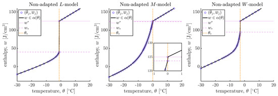
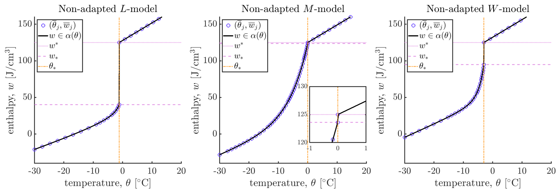
Figure 7 shows an illustration of Algorithm 12 with $J=24$, $w_{tol}=5[\mathrm{J}/{\mathrm{cm}}^3]$. We require refinements $m_{ref}\in \{4,5,5\}$ for the non-adapted $L,M,W$-models, respectively.

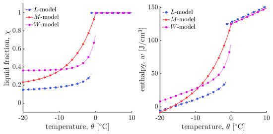
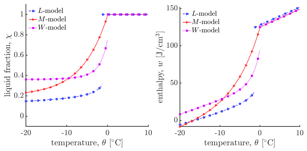
Figure 7. Illustration of lookup points $({\overline{\theta }}_j,{\overline{w}}_j)\in \tilde{\alpha }[{\theta }_{*},{\chi }_{*},\mathrm{{\rm Y}}]$ from Example 2 using non-adapted models L, M, and W. We have used an initial $J=24$ and $w_{tol}=5[\mathrm{J}/{\mathrm{cm}}^3]$ with a maximum number of $m_{ref}=5$ refinements.

Remark 6.

To find an initial bracket for the local nonlinear solver, we must be given some w. Then, we find the first $j:{\overline{w}}_j\le w$ and set ${\theta }_{left}={\overline{\theta }}_j$ and ${\theta }_{right}={\overline{\theta }}_{j+1}$.

Remark 7.

We choose the midpoint of the bracket in Remark 6 for any local nonlinear solver that requires an initial guess.

5.5. Choosing the Representative Jacobian for Solving (39b)

We now provide the details to identify the Clarke’s generalized Jacobian from Step 5 in Algorithm 8 for the ($P^{*}$) model considered in this paper.

Given $W_j$, we choose the representative element $D_W\left({\mathrm{\Theta }}_j\right)$ of the Jacobian $D_W\left(\mathrm{\Theta }\right)$, which is diagonal as

$$\begin{array}{c}\hfill \left\{\begin{array}{cccc}\mathrm{when}{W}_j\ge w_{*}:\hfill & \hfill D_W\left({\mathrm{\Theta }}_j\right)& =& {\left[{\left(w_{-}\right)}^{\prime }\left({\mathrm{\Theta }}_j\right)\right]}^{-1}\hfill \\ \mathrm{when}{w}_{*}<W_j<w^{*}:\hfill & \hfill D_W\left({\mathrm{\Theta }}_j\right)& =& 0,\hfill \\ \mathrm{when}{W}_j\ge w^{*}:\hfill & \hfill D_W\left({\mathrm{\Theta }}_j\right)& =& c_{uf}^{-1},\hfill \end{array}\right.\end{array}$$

(45)

where ${\left(w_{-}\right)}^{\prime }\left(\theta \right)$ is given by

$$\begin{array}{c}\hfill {\left(w_{-}\right)}^{\prime }\left(\theta \right)=c_{uf}+(c_{fr}-c_{uf})(\mathrm{{\rm Y}}\left(\theta \right)-\mathrm{{\rm Y}}\left({\theta }_{*}\right))+\eta (1-S_g)L{\mathrm{{\rm Y}}}^{\prime }\left(\theta \right).\end{array}$$

(46)

We provide the auxiliary calculations for (46) in Table A2.

6. Results

In this Section, we evaluate algorithms from Section 4 and Section 5 to solve (21), a nonlinear algebraic problem that needs to be solved at every time step n of a simulation of heat equation with generalized constitutive laws.

In our examples, we choose parameters which are physically realistic and appropriate for a permafrost simulation scenario. In particular, we compare how the algorithms behave for the more challenging ($P^{*}$) model as compared to the (P) model, which presents fewer challenges.

We study and evaluate the local and global solvers. The usual metric of evaluation of solvers is the computational cost: (i) one strives to have as few iterations as possible needed for convergence, (ii) one wants to guarantee the convergence, and (iii) one attempts to keep the cost per iteration to a minimum. While the Newton iteration requires closeness to the initial guess for convergence, (ii) is not achievable in principle, but in time-dependent problems, one can implement the time-step cutting to keep the initial guesses for a time step reasonably close to the true solution of (21a), thus guaranteeing (i) but requiring more time steps. In addition, some modifications of the Newton iteration such as inexact or quasi-Newton [17] are useful for (iii) but incur additional iterations and contradict (i).

In the simulation studies of complex models such as the ($P^{*}$) model, of interest is also the (iv) robustness of solvers. In particular, a local solver should be robust so that an investment in the evaluation of residual and Jacobian of the global solver is not wasted if the local solver fails at some j.

In Section 6.1, we discuss the local problem (21b) and specifically (13) for the ($P^{*}$) compared to (P) models. Based on these studies, we postulate that Ridders’ algorithm outperforms every other local solver we considered. In Section 6.2, we study grid-convergence and compare the approaches from Section 5.3 for handling the discrete diffusion operator. Based on this study, Algorithm 10 could be useful in certain situations where a slightly higher accuracy is desired, but the cost per (global) iteration is higher. In Section 6.3, we study the performance of Algorithm 8. In Section 6.4, we compare the initialization of Algorithm 8 with and without the extrapolation proposed in Algorithm 9. Based on these studies, we recommend that Algorithm 9 should be used for challenging $\left(P^{*}\right)$ models, such as with the L-model.

Remark 8.

Since $w\in \alpha \left(\theta \right)$ is semi-smooth on its full domain $\mathbb{R}$, any Newton-based algorithm we apply is really semi-smooth, i.e., it is based on Algorithm 3 or its extensions. In some instances, however, we only work with a portion of the domain on which $\alpha \left(\theta \right)$ is smooth; thus, we refer to Algorithm 1. In the comparisons reported in this Section, we refer to Algorithms 1 and 3 interchangeably.

6.1. Solving the Local Problem

We focus here on the local problem (21b) and specifically (13), i.e., given w, inverting $\psi \left(w\right)=(\theta ,\chi )$ in (11).

The relationship (11) involves parameters ${\theta }_{*},{\chi }_{*}$, and a function $\mathrm{{\rm Y}}(·)$. We consider both the non-adapted parameters for ($P^{*}$) model as well as the simpler (P) model, which uses the smoother adapted relationships. The data for these parameters is, respectively, in Table 2 and Table 3.

Table 3. Data for adapted models for (4) from the mathematical literature [10], which also draws from geophysical literature [5,6,8]. The parameter values correspond to clay. Observe that ${\chi }_{*}=1$ here.

Model	Parameter Values	${\mathit{\chi }}_{*}$	Ref.
$\left(L\right)$	$a=1[-]$, $b=0.271\left[1{/}^{\circ }\mathrm{C}\right]$, ${\theta }_{*}=-1.1544{[}^{\circ }\mathrm{C}]$	$1[-]$	[10]
$\left(M\right)$	$a=1[-]$, $b=0.16\left[1{/}^{\circ }\mathrm{C}\right]$, ${\chi }_{res}=0.20144[-]$	$1[-]$	[10]
$\left(W\right)$	$a=0.64[-]$, $b=6.4216{[}^{\circ }\mathrm{C}]$, ${\chi }_{res}=0.36[-]$,	$1[-]$	[10]

Once we fix the data for $\mathcal{G}(·),\alpha (·)$ in (4), we construct $w\in \alpha (·)$ and compute the corresponding $w_{min}$, $w_{max}$. Then, we consider several values $w_{step}$ distributed uniformly in $w_{step}\in [w_{min},w_{max}]$.

For each $w_{step}$, we test a local solver to solve (11)

$$\begin{array}{c}\hfill \psi \left(w_{step}\right)=({\theta }_{step},{\chi }_{step}).\end{array}$$

(47)

We consider solvers from the following list: Newton Algorithm 1, Newton–Anderson Algorithm 2, Ridders’ Algorithm 6 from Section 4.2.1 and Secant Algorithm 7 from Section 4.2.2. We also use Algorithms 11 and 12 to initialize the iterations.

Example 2.

Consider thermal and soil parameters from Table 4. Choose a priori the range of temperature $\theta \in V_{\theta }=[{\theta }_{min},{\theta }_{max}]=[-30,20]{[}^{\circ }\mathrm{C}]$. This $V_{\theta }$ allows, in particular, time-varying boundary conditions realistic for atmospheric conditions in the Arctic.

Table 4. Thermal parameters.

$\mathit{\eta }$	${\mathit{S}}_{\mathit{g}}$	L	${\mathit{c}}_{\mathit{i}}$	${\mathit{c}}_{\mathit{l}}$	${\mathit{c}}_{\mathit{r}}$	${\mathit{c}}_{\mathit{g}}$	${\mathit{k}}_{\mathit{i}}$	${\mathit{k}}_{\mathit{l}}$	${\mathit{k}}_{\mathit{r}}$	${\mathit{k}}_{\mathit{g}}$
0.43	0.05	306	1.90	4.19	1.21	0.000927	0.0230	0.0058	0.0025	0.00026

With $\theta \in V_{\theta }$, we find the range $V_w=[w_{min},w_{max}]$ for the ($P^{*}$) model with non-adapted data from Table 2, and we calculate the following range for $w\in V_w$

$$\begin{array}{c}\hfill \begin{array}{cccc}L\text{-}\mathit{model}:\hfill & \hfill w_{step}& \in & [-5.767,151.789][\mathrm{J}/{\mathrm{cm}}^3];\hfill \\ M\text{-}\mathit{model}:\hfill & \hfill w_{step}& \in & [-8.357,149.014][\mathrm{J}/{\mathrm{cm}}^3];\mathit{and}\hfill \\ W\text{-}\mathit{model}:\hfill & \hfill w_{step}& \in & [10.156,151.416][\mathrm{J}/{\mathrm{cm}}^3].\hfill \end{array}\end{array}$$

(48)

For the (P) model with data in Table 3, we have

$$\begin{array}{c}\hfill \begin{array}{cccc}L\text{-}\mathit{model}:\hfill & \hfill w_{step}& \in & [40.466,151.789][\mathrm{J}/{\mathrm{cm}}^3];\hfill \\ M\text{-}\mathit{model}:\hfill & \hfill w_{step}& \in & [-8.316,149.014][\mathrm{J}/{\mathrm{cm}}^3];\mathit{and}\hfill \\ W\text{-}\mathit{model}:\hfill & \hfill w_{step}& \in & [7.96362,149.014][\mathrm{J}/{\mathrm{cm}}^3].\hfill \end{array}\end{array}$$

(49)

We compare the robustness and convergence of the local solvers to invert

$$\begin{array}{c}\hfill \psi \left(w_{step}\right)=({\theta }_{step},{\chi }_{step})\end{array}$$

(50)

where $w_{step}$ are in the range $V_w$ appropriate for a given constitutive model. We use ${\tau }_a={10}^{-12}$ in (Stopping Criterium). To initialize the iterations, we set $\gamma =1$ in Algorithm 11. We also consider Algorithm 12 with ${\theta }_{min}=-30{[}^{\circ }\mathrm{C}]$ and ${\theta }_{max}=20{[}^{\circ }\mathrm{C}]$ with $J=50$, and $w_{tol}=0.5[\mathrm{J}/{\mathrm{cm}}^3]$.

In Table 5, we report the maximum iterations required for each solver to converge for the different algorithms and variants of initialization we consider.

Table 5. Results of Example 2: the number of iterations required to solve the local problem $\psi \left(w_{step}\right)=({\theta }_{step},{\chi }_{step})$ for the ($P^{*}$) (top, (A)), and (P) models (bottom, (B)), with constitutive models L, M, and W, and $w_{step}$ from the range $V_w$ given by (48) and (49), respectively. We present the maximum of the number of iterations over all $w_{step}$ for each case. For each solver, we also test the initialization strategy called “look-up” (Algorithm 12) and find the initial “bracket” (Algorithm 11). We use ${\tau }_a={10}^{-12}$ with $k^{max}=20$ for the local and global stopping criteria. We use $J=50$, $w_{tol}=0.5[\mathrm{J}/{\mathrm{cm}}^3]$ and up to $m_{ref}=10$ refinements for the adaptive look-up table. There was no stopping criteria used for the bracketing algorithm because Algorithm 11 terminates once the bracket is found; see (Section 9, Remark 27, [37]).

(A) Results for (${\mathit{P}}^{\mathbf{*}}$) model.
Local solver	Ridders’		Secant		Newton		Newton-Anderson
	Look-Up	Bracket	Look-Up	Bracket	Look-Up	Bracket	Look-Up	Bracket
L-model	2	3	4	6	8	8	3	5
M-model	2	3	4	6	2	4	3	6
W-model	2	3	4	7	2	4	3	6
(B) Results for ($\mathit{P}$) model.
Local solver	Ridders’		Secant		Newton		Newton-Anderson
	Look-Up	Bracket	Look-Up	Bracket	Look-Up	Bracket	Look-Up	Bracket
L-model	2	3	4	7	13	13	3	6
M-model	2	3	4	6	2	4	3	6
W-model	2	3	4	7	2	4	3	7

Discussion

We see that Ridders’ method is the most robust solver, with the initial bracket found by Algorithm 12 and chosen in accordance to Remark 6. Its performance is on par with that of the Newton–Anderson method Algorithm 2 with depth size $m=1$, with Algorithm 12 and an initial guess as suggested by Remark 7.

Overall, the results from Table 5 suggest that Ridders’ method results in the fewest iterations required to converge. Similar results are reported when ${\tau }_a={10}^{-8}$, where the initial bracket is found by Remark 6 in (Table 9.11, [37]).

In turn, for Newton’s method applied to solve (50) for the ($P^{*}$) non-adapted and (P) adapted L-models, it is comparable between Algorithm 12 and Algorithm 11. However, for the $M,W$-models, we see that Newton’s method combined with the initial guess from Remark 7 is the second most robust choice of local nonlinear solver.

6.2. Grid Convergence and Use of Iteration Lagging

First, we report on grid convergence of our numerical solver for the ($P^{*}$) model. These results are new; see more detailed reports in [37].

Example 3.

Let $\mathrm{\Omega }=(0,20)\left[\mathrm{m}\right]$ with $h=\{1.25,2.5,5,10,20\}\left[\mathrm{cm}\right]$ and time step $\tau =1440 h\left[\mathrm{s}\right]$ with $t\in (0,365]\left[\mathrm{d}\right]$. We approximate the solutions to ($P^{*}$) model (2) with the non-adapted W-model from (4c) with parameters for clay in Table 2 and thermal parameters from Table 4. We use smooth time-varying Dirichlet boundary conditions at the surface

$$\begin{array}{ccc}\hfill \theta (0,t)={\theta }_{smooth}\left(t\right)=4-10\cos \left(\frac{2\pi (t+100)}{337}\right){[}^{\circ }\mathrm{C}],& & t\in (0,365]\left[\mathrm{d}\right],\hfill \end{array}$$

(51)

and set $\theta (20,t)=-0.111{[}^{\circ }\mathrm{C}]$ to represent the isothermal layer of permafrost soils. The initial conditions are ${\theta }_{init}\left(x\right)=-0.111{[}^{\circ }\mathrm{C}]$ for all $x\in \mathrm{\Omega }$ at time $t=0$.

We simulate this scenario with Algorithms 8 and 10 and evaluate the space-time grid error using the norms $\Vert {(u(x_j,t_n)-U_j^n)}_{j,n}{\Vert }_{\infty ,p}$ for different variables u from $u=(\theta ,\chi ,w)$. Of course, we do not know the “true” solution. Thus, we use a fine-grid solution as a proxy for the unknown true solution to Example 3.

6.2.1. Grid Convergence and Time-Lagging Discrete Diffusion

The grid convergence results are given in Table 6 and show the expected low order, appropriate for low regularity solutions and a formally first order scheme. We see an optimal grid convergence of order better than 1 in the “$\infty ,1$” norm and roughly of order 1 in the “$2,2$” norm. The rates in the “$\infty ,2$” norm are less forgiving even in $\theta$, which is a smoother variable.

Table 6. Order of convergence from Example 3 obtained by Algorithm 8 that is with time-lagging, ${\mathsf{\ell }}_{max}=1$ (top) and ${\mathsf{\ell }}_{max}=5$ (bottom). The order remains similar (not shown) when ${\mathsf{\ell }}_{max}=15$, suggesting the difference of solutions due to iteration on $\mathcal{A}$ is insignificant. We use ${\tau }_a={10}^{-8}$, $h=\{1.25,2.5,5,10,20\}\left[\mathrm{cm}\right]$ and time step $\tau =1440 h\left[\mathrm{s}\right]$ with $t\in (0,365]\left[\mathrm{d}\right]$.

Norm	$\mathit{w}$	$\mathit{\theta }$	$\mathit{\chi }$
$\Vert ·{\Vert }_{\infty ,1}$	1.4471	1.1559	1.4580
$\Vert ·{\Vert }_{\infty ,2}$	0.6996	0.6551	0.6951
$\Vert ·{\Vert }_{2,2}$	1.0960	1.3266	1.0895
Norm	$\mathit{w}$	$\mathit{\theta }$	$\mathit{\chi }$
$\Vert ·{\Vert }_{\infty ,1}$	1.4434	1.2287	1.4555
$\Vert ·{\Vert }_{\infty ,2}$	0.7025	0.7289	0.6981
$\Vert ·{\Vert }_{2,2}$	1.0907	1.3234	1.0842

We recall that a fully implicit formulation in (37) requires handling the nonlinear dependence of the discrete diffusion matrix $\mathcal{A}=\mathcal{A}\left({\mathrm{\Theta }}^n\right)$ on one of the unknowns of the system. Algorithm 8 uses time-lagging and an alternative approach. Algorithm 10 uses an external iteration of ${\mathsf{\ell }}_{max}$ iterations so that Algorithm 8 corresponds to ${\mathsf{\ell }}_{max}=1$. We compare these now.

We consider ${\mathsf{\ell }}_{max}=1$ and ${\mathsf{\ell }}_{max}=5$, with the results reported again in Table 6. We also consider ${\mathsf{\ell }}_{max}=15$, but the results are almost identical to those for ${\mathsf{\ell }}_{max}=5$; thus, we do not report these. In the end, we do not see a significant difference for the order of convergence between ${\mathsf{\ell }}_{max}=1$ and ${\mathsf{\ell }}_{max}=5$, which seems to suggest that iterating beyond ${\mathsf{\ell }}_{max}=5$ is not needed. Our overall impression is also that the impact of time-lagging is minor; thus, its use is reasonable.

6.2.2. Impact of Time-Lagging

Next, we revisit the impact of the choice of time-lagging in Algorithm 8 versus the use of iteration in Algorithm 10 on the pointwise values of $w,\theta ,\chi$. Considering pointwise values is clearly a less forgiving metric than that reported in Table 6. In particular, it is known that the discretization we employ of mixed finite element methods is less accurate for Dirichlet conditions than nodal based discretizations, and this feature is exacerbated for time dependent problems with large discrepancy between the initial and boundary conditions, as well as for significant or non-smooth nonlinearity.

We define the relative error in a variable u defined as

$$\begin{array}{c}\hfill E(u;h)=\underset{n}{\max }\left({\displaystyle \frac{\Vert u_h^n-{\widehat{u}}_h^n{\Vert }_{\infty }}{\Vert u_h^n{\Vert }_{\infty }}}\right),\end{array}$$

(52)

where ${\widehat{u}}_h^n$ is the solution using iteration-lagging with Algorithm 10, and $u_h^n$ is the numerical solution using time-lagging with Algorithm 8. We evaluate $E(u,h)$ for the ($P^{*}$) model, where u denotes one of the variables $w,\theta ,\chi$.

We expect that the impact of time-lagging of $\mathcal{A}$ might be significant for a coarse grid and near the boundary for the initial transients when using dramatically varying boundary conditions such as in Example 3. This is confirmed by the results reported in Table 7. We see a large impact on the discrepancy of pointwise values of ${\mathrm{\Theta }}^n$ even with ${\mathsf{\ell }}_{max}=5$ near the boundary and when $n\approx 1$. This effect diminishes when $n\ge 10$ is only considered.

Table 7. Relative error $E(·;h)$ given by (52) from Example 3 for variable $u\in \{w,\theta ,\chi \}$ when ${\mathsf{\ell }}_{max}=5$. Top: results for $n=1,\dots N$ show significant impact of iteration on the variable $\theta$. Bottom: results for $n=11,\dots N$ show the impact diminishes in time. We use ${\tau }_a={10}^{-8}$, $h=\{1.25,2.5,5,10,20\}\left[\mathrm{cm}\right]$ and time step $\tau =1440 h\left[\mathrm{s}\right]$ with $t\in (0,365]\left[\mathrm{d}\right]$.

$\mathit{h}\left[\mathbf{cm}\right]$	$\mathit{w}$	$\mathit{\theta }$	$\mathit{\chi }$
20	0.00384177	1.0000	0.00384177
10	0.0073728	0.448556	0.00737283
5	0.0146504	0.231464	0.0146503
2.5	0.0296403	0.173759	0.0296403
1.25	0.0214733	0.27838	0.0231336
$\mathit{h}\left[\mathbf{cm}\right]$	$\mathit{w}$	$\mathit{\theta }$	$\mathit{\chi }$
20	0.00241073	0.102111	0.00182218
10	0.0031226	0.048945	0.00341837
5	0.00601393	0.0408784	0.00655036
2.5	0.00784449	0.0338697	0.00868233
1.25	0.0119784	0.0317058	0.0133408

These results show that while grid convergence is achieved, the impact of time-lagging on the simulation scenarios where pointwise values near the boundary are required might be significant. Such is the case, e.g., for coupled problems such as those reported in [15,16].

6.3. Performance of Solvers When Working with Realistic Boundary Conditions

Having established that the algorithms give solutions that seem to converge as well as seem robust, we are ready to make recommendations on the performance of global solvers.

Specifically, we aim to compare the performance of traditional Newton-based Algorithms 1 and 3 to our Newton–Anderson-based Algorithm 8 when using realistic rough data or smooth data. Specifically, we choose to test the solvers with highly varying boundary conditions corresponding to annual variations of temperature. Our focus is on the ($P^{*}$) model. See the results on the much smoother (P) model and Algorithm 1 in e.g., [9,11].

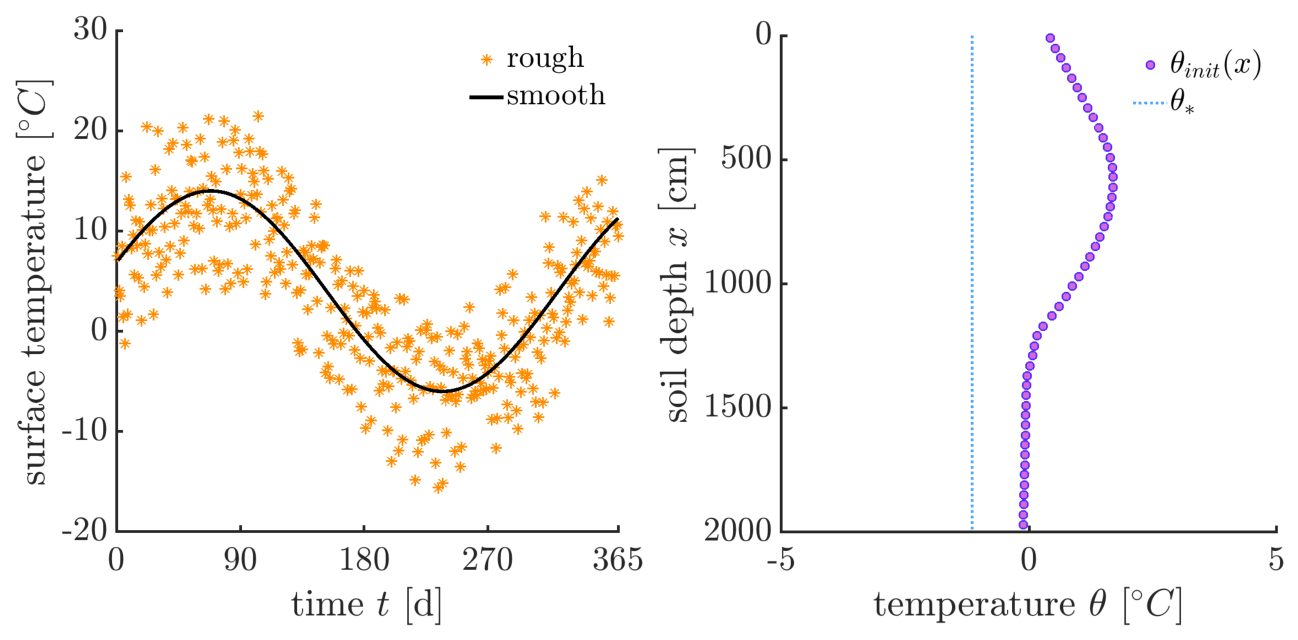
We use the keyword “rough” to refer to the uncertain but realistic boundary conditions and use the keyword “smooth” when using their continuous average given by (51) with

$$\begin{array}{c}\hfill {\theta }_{rough}\left(t\right)={\theta }_{smooth}\left(t\right)+\mathcal{N}(0,{10}^2){[}^{\circ }\mathrm{C}],t\in (0,1)\left[\mathrm{yr}\right],\end{array}$$

(53)

See Figure 8 for illustration of one realization of (53). More discussion on the uncertainty is in (Section 10.3, [37]) and in [58].

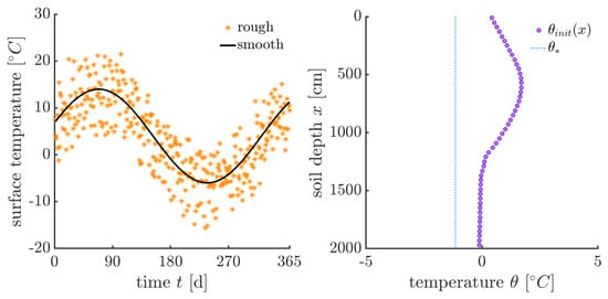
Figure 8. (Left): rough and smooth boundary conditions (53) used in Example 4 and (right): initial conditions data [59]. We use ${\tau }_a={10}^{-8}$, $h=20\left[\mathrm{cm}\right]$, $\tau =1\left[\mathrm{d}\right]$ with $T=1\left[\mathrm{yr}\right]$.

Example 4.

Let $\mathrm{\Omega }=(0,20)\left[\mathrm{m}\right]$. We consider the ($P^{*}$) model with the non-adapted L-model for Example 4 because it is the hardest model for Newton-based computational algorithms to handle. We use the thermal parameters from Table 4.

We use the Dirichlet time-varying boundary conditions $\theta (0,t)={\theta }_{smooth}\left(t\right)$ from (51) or (53) supplemented with $\theta (20,t)=-0.111{[}^{\circ }\mathrm{C}]$. We take initial conditions extrapolated from data [59]; see the plot in Figure 8.

We discretize the problem with $h=20\left[\mathrm{cm}\right]$ and use a time step of $\tau =1\left[\mathrm{d}\right]$ with $T=1\left[\mathrm{yr}\right]$.

We apply Algorithm 1 as well as Algorithm 8 with ${\tau }_a={10}^{-8}$, which are supplemented with Algorithm 12.

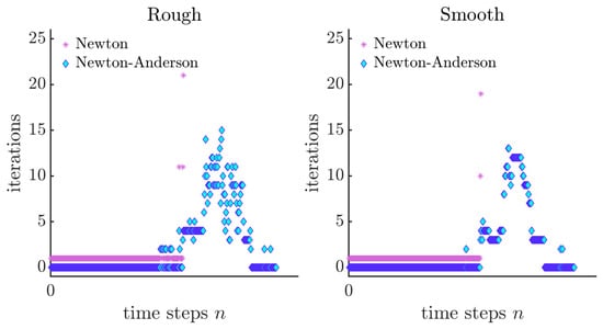
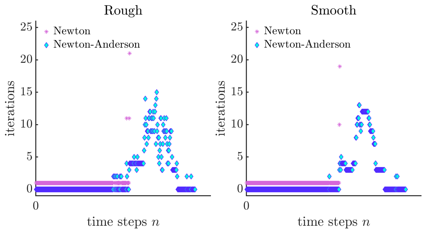
We compare the performance of the Newton Algorithm 1, which in this semismooth setting is Algorithm 3 for the ($P^{*}$) model. In Figure 9, we provide plots of the number of iterations required for convergence over all time steps. We see that maximum number of iterations $k=k^{max}=20$ is reached for Algorithm 1 about the time when temperatures switches from warm to cold in the middle of the simulation scenario. This is the hardest case and the solver based on Algorithm 1 does not converge for either the smooth or rough boundary conditions.

Figure 9. Results for Example 4: maximum number of iterations required per time step depending on solver choice, boundary conditions. (Left): implementation of rough and (right): smooth boundary conditions. We use a stopping criteria of ${\tau }_a={10}^{-8}$ with $k^{max}=20$.

However, Algorithm 8 based on the Newton–Anderson Algorithm 5 with depth $m=1$ is more robust, since it required only $k=15$ and $k=13$, respectively, for the rough and smooth boundary conditions. We note that Algorithm 8 uses a depth size of $m=1$.

We also consider $m>1$ in Algorithm 2, which improves substantially the performance and requires at most $k=6$ iterations over all time steps. However, for depth $m=3$, we do not see further improvement. Hence, small depth sizes for global solvers offer most robust and efficient solvers.

6.4. Comparison of Initialization Methods for the Global Solver

We now compare the initialization strategy of the choice of initial guesses in Algorithm 8 without extrapolation and with extrapolation, as in Algorithm 9.

Example 5.

Let $\mathrm{\Omega }=(0,20)\left[\mathrm{m}\right]$. Unless otherwise stated, we use model parameters as in Example 3. We discretize with $h=20\left[\mathrm{cm}\right]$ and $\tau =3\left[\mathrm{hr}\right]$ with $T=1\left[\mathrm{yr}\right]$ and use ${\tau }_a={10}^{-8}$.

We use the time-varying Dirichlet boundary conditions

$$\begin{array}{ccc}\hfill \theta (0,t)=-5+15\sin \left(2\pi t\right){[}^{\circ }\mathrm{C}],& \theta (20,t)=-5{[}^{\circ }\mathrm{C}],& t\in (0,1)\left[\mathrm{yr}\right],\hfill \end{array}$$

(54)

and set initial conditions equal to ${\theta }_{init}\left(x\right)=-5{[}^{\circ }\mathrm{C}]$. These are the same underlying smooth boundary conditions considered in (Example 6.3, [11]).

We employ Algorithm 8 or Algorithm 9, which are both supplemented with Algorithm 12.

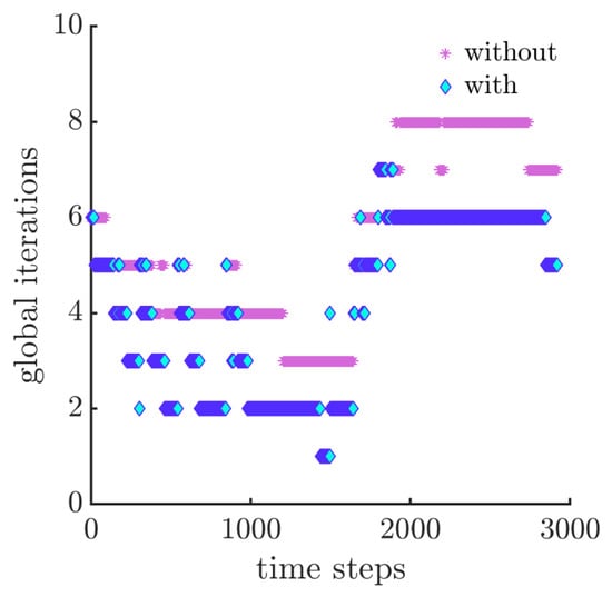
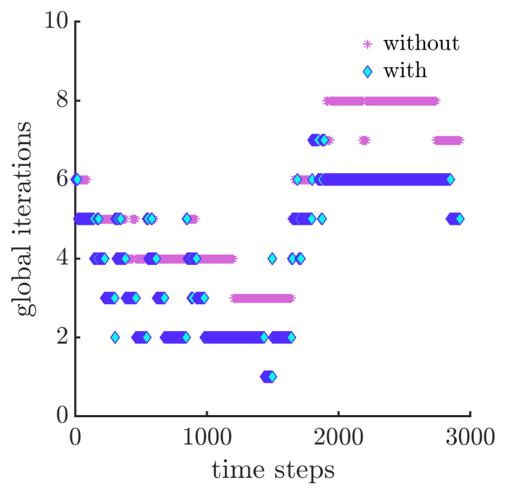
We plot the results in Figure 10. We see that we obtain a speed up of about two iterations when using Algorithm 9 compared to when we do not use the extrapolation. With the other data reported here, we have found that Algorithm 9 may provide a speed up of at least one iteration.

Figure 10. Results of Example 5: maximum number of iterations required over all time steps. The keyword “without” and “with” means that we have either used Algorithm 8 or Algorithm 9, respectively. We use a stopping criteria of ${\tau }_a={10}^{-8}$ with $k^{max}=20$.

Remark 9

(Time steps and spatial discretizations). The non-adapted L-model is the hardest constitutive model for any Newton-based computational algorithms. When starting from sub-freezing initial conditions, the solver requires small time steps of $\tau \le 6\left[\mathrm{hr}\right]$; see (Section 11, Table 11.8, [37]). This is in contrast to above-freezing initial conditions; these allow for larger time steps of $\tau \le 1\left[\mathrm{d}\right]$. At the same time, the M- and W- models allow for larger time-steps of, respectively, $\tau \le 31\left[\mathrm{d}\right]$ and $\tau \le 25\left[\mathrm{d}\right]$ (Section 11, Table 11.8, [37]). In each, we have found that using $h=20\left[\mathrm{cm}\right]$ suffices when considering $\mathrm{\Omega }=(0,20)\left[\mathrm{m}\right]$.

7. Conclusions

In this paper, we presented and evaluated advanced algorithms to simulate a complex model called ($P^{*}$) given by (2) for modeling realistic permafrost scenarios. Our focus was on nonlinear solvers, and we proposed new algorithms in Section 4 and Section 5. We evaluated the performance of these algorithms focusing on the specific challenges of the $\left(P^{*}\right)$ models. We aimed to evaluate, in particular, the computational cost of these algorithms resulting from the number of iterations required for convergence, as well as their robustness.

We studied both local and global solvers. We found that Ridders’ method was the most robust choice for the local solver and that the use of adaptive look-up tables, i.e., Algorithm 12, provided the most robust initial bracket or initial guesses for the various (local) nonlinear solvers considered here.

For the global solver, we evaluated our newly proposed Algorithm 8 based on Newton–Anderson algorithm implemented in the semi-smooth setting, which appears new to this class of algorithms. This algorithm outperforms the Newton algorithm and is best for use with moderate depth $m\le 2$. We find that it worked well in particular for some challenging cases where the Newton algorithm might fail.

We also proposed and evaluated several other algorithmic refinements, including the best ways to initialize the guesses. Some have significant and some have less significant impact on the performance. In the end, we recommend to implement a simple look-up algorithm, Algorithm 12, which helps to provide a good initial guess for the local solver, as well as Algorithm 9, which helps to provide an improved guess for the global solver. We also studied effects of time-lagging of discrete diffusion operator and found through Algorithm 10 that it does not offer a substantial gain in the order of convergence while it has high computational cost.

References

- Osterkamp, T.; Burn, C. PERMAFROST. In Encyclopedia of Atmospheric Sciences; Holton, J.R., Ed.; Academic Press: Oxford, UK, 2003; pp. 1717–1729. [Google Scholar] [CrossRef] [Scilit]
- Sandells, M.; Flocco, D. Introduction to the Physics of the Cryosphere; Morgan and Claypool: San Rafael, CA, USA, 2014. [Google Scholar]
- Romanovsky, V.; Osterkamp, T. Effects of unfrozen water on heat and mass transport in the active layer and permafrost. Permafr. Periglac. Process. 2000, 11, 219–239. [Google Scholar] [CrossRef] [Scilit]
- Osterkamp, T.E.; Jorgenson, M.T.; Schuur, E.A.G.; Shur, Y.L.; Kanevskiy, M.Z.; Vogel, J.G.; Tumskoy, V.E. Physical and ecological changes associated with warming permafrost and thermokarst in Interior Alaska. Permafr. Periglac. Process. 2009, 20, 235–256. [Google Scholar] [CrossRef] [Scilit]
- Andersland, O.B.; Ladanyi, B. Frozen Ground Engineering, 2nd ed.; Wiley: Hoboken, NJ, USA; ASCE: Reston, VA, USA, 2004. [Google Scholar]
- Ling, F.; Zhang, T. A numerical model for surface energy balance and thermal regime of the active layer and permafrost containing unfrozen water. Cold Reg. Sci. Technol. 2004, 38, 1–15. [Google Scholar] [CrossRef] [Scilit]
- Nicolsky, D.J.; Romanovsky, V.E.; Alexeev, V.A.; Lawrence, D.M. Improved modeling of permafrost dynamics in a GCM land-surface scheme. Geophys. Res. Lett. 2007, 34, L08501. [Google Scholar] [CrossRef] [Scilit]
- Garayshin, V.; Nicolzsky, D.; Romanovsky, V. Numerical modeling of two-dimensional temperature field dynamics across non-deforming ice-wedge polygons. Cold Reg. Sci. Technol. 2019, 161, 115–128. [Google Scholar] [CrossRef] [Scilit]
- Bigler, L.; Peszynska, M.; Vohra, N. Heterogeneous Stefan problem and permafrost models with P0-P0 finite elements and fully implicit monolithic solver. Electron. Res. Arch. 2022, 30, 1477–1531. [Google Scholar] [CrossRef] [Scilit]
- Peszynska, M.; Vohra, N.; Bigler, L. Upscaling an extended heterogeneous Stefan problem from the pore-scale to the Darcy scale in permafrost. Multiscale Model. Simul. 2024, 22, 436–475. [Google Scholar] [CrossRef] [Scilit]
- Vohra, N.; Peszynska, M. Robust conservative scheme and nonlinear solver for phase transitions in heterogeneous permafrost. J. Comput. Appl. Math. 2024, 442, 115719. [Google Scholar] [CrossRef] [Scilit]
- Hansson, K.; Simunek, J.; Mizoguchi, M.; Lundin, L.C.; Van Genuchten, M. Water Flow and Heat Transport in Frozen Soil. Vadose Zone J. 2004, 3, 527–533. [Google Scholar] [CrossRef] [Scilit]
- Nicolsky, D.J.; Romanovsky, V.E.; Tipenko, G.S.; Walker, D.A. Modeling biogeophysical interactions in nonsorted circles in the Low Arctic. J. Geophys. Res. Biogeosci. 2008, 113, G03S05. [Google Scholar] [CrossRef] [Scilit]
- Zhang, Y.; Michalowski, R. Thermal-Hydro-Mechanical Analysis of Frost Heave and Thaw Settlement. J. Geotech. Geoenviron. Eng. 2015, 141, 04015027. [Google Scholar] [CrossRef] [Scilit]
- Vohra, N.; Peszynska, M. Iteratively coupled mixed finite element solver for thermo-hydro-mechanical modeling of permafrost thaw. Results Appl. Math. 2024, 22, 100439. [Google Scholar] [CrossRef] [Scilit]
- Peszynska, M.; Hilliard, Z.; Vohra, N. Coupled flow and energy models with phase change in permafrost from pore- to Darcy scale: Modeling and approximation. J. Comput. Appl. Math. 2024, 450, 115964. [Google Scholar] [CrossRef] [Scilit]
- Kelley, C.T. Iterative Methods for Linear and Nonlinear Equations; SIAM: Philadelphia, PA, USA, 1995. [Google Scholar]
- Atkinson, K.; Han, W. Theoretical Numerical Analysis: A Functional Analysis Framework; Springer: New York, NY, USA, 2005. [Google Scholar]
- Dennis, J.E., Jr.; Schnabel, R.B. Numerical Methods for Unconstrained Optimization and Nonlinear Equations; SIAM: Philadelphia, PA, USA, 1996. [Google Scholar]
- Stoer, J.; Bulirsch, R. Introduction to Numerical Analysis; Springer: New York, NY, USA, 1991. [Google Scholar]
- Pollock, S.; Rebholz, L. Anderson Acceleration for Numerical PDEs; SIAM Spotlights; SIAM: Philadelphia, PA, USA, 2025. [Google Scholar]
- Pollock, S.; Schwartz, H. Benchmarking results for the Newton-Anderson method. Results Appl. Math. 2020, 8, 100095. [Google Scholar] [CrossRef] [Scilit]
- Toth, A.; Kelley, C.T. Convergence analysis for Anderson acceleration. SIAM J. Numer. Anal. 2015, 53, 805–819. [Google Scholar] [CrossRef] [Scilit]
- Evans, C.; Pollock, S.; Rebholz, L.G.; Xiao, M. A proof that Anderson acceleration improves the convergence rate in linearly converging fixed-point methods (but not in those converging quadratically). SIAM J. Numer. Anal. 2020, 58, 788–810. [Google Scholar] [CrossRef] [Scilit]
- Ulbrich, M. Semismooth Newton Methods for Variational Inequalities and Constrained Optimization Problems in Function Spaces; SIAM: Philadelphia, PA, USA, 2011. [Google Scholar]
- Hintermüller, M.; Ito, K.; Kunisch, K. The primal-dual active set strategy as a semismooth Newton method. SIAM J. Optim. 2002, 13, 865–888. [Google Scholar] [CrossRef] [Scilit]
- Peszynska, M.; Mathangadeera, P.; Phelps, M.; Felsch, F.; Unger-schulz, N. Heat conduction with phase change in soils with macro-pores, snow, and cryoconite. Part I: Unified model derivation and examples. SeMA 2025, 82, 595–632. [Google Scholar] [CrossRef] [Scilit]
- Rogers, J.C.; Berger, A.E.; Ciment, M. The alternating phase truncation method for numerical solution of a Stefan problem. SIAM J. Numer. Anal. 1979, 16, 563–587. [Google Scholar] [CrossRef] [Scilit]
- Verdi, C.; Visintin, A. Error estimates for a semi-explicit numerical scheme for Stefan-type problems. Numer. Math. 1988, 52, 165–185. [Google Scholar] [CrossRef] [Scilit]
- Nochetto, R.H.; Verdi, C. The combined use of a nonlinear Chernoff formula with a regularization procedure for two-phase Stefan problems. Numer. Funct. Anal. Optim. 1987, 9, 1177–1192. [Google Scholar] [CrossRef] [Scilit][Green Version]
- Knabner, P.; Angermann, L. Numerical Methods for Elliptic and Parabolic Partial Differential Equations; Springer: Cham, Switzerland, 2003. [Google Scholar]
- Du, Q.; Feng, X. Chapter 5—The phase field method for geometric moving interfaces and their numerical approximations. In Geometric Partial Differential Equations—Part I; Handbook of Numerical Analysis; Bonito, A., Nochetto, R.H., Eds.; Elsevier: Amsterdam, The Netherlands, 2020; Volume 21, pp. 425–508. [Google Scholar] [CrossRef] [Scilit]
- Yin, F.; Xu, Z.; Fu, Y. Novel high-order explicit energy-preserving schemes for NLS-type equations based on the Lie-group method. Math. Comput. Simul. 2024, 225, 570–585. [Google Scholar] [CrossRef] [Scilit]
- Kutz, J.N. Data-Driven Modeling & Scientific Computation: Methods for Complex Systems & Big Data; Oxford University Press: Oxford, UK, 2026. [Google Scholar]
- Bramburger, J.J. Data-Driven Methods for Dynamic Systems; SIAM: Philadelphia, PA, USA, 2024. [Google Scholar]
- Calmels, F.; Clavano, W.; Froese, D. Progress on X-ray computed tomography (CT) scanning in permafrost studies. In Proceedings of the 5th Canadian Conference on Permafrost, GEO2010, Calgary, AB, Canada, 12–15 September 2010; pp. 1353–1358. [Google Scholar]
- Phelps, M. Mathematical and Computational Aspects of Nonlinear Heat Conduction Models with Generalized Consitutive Laws. Ph.D. Thesis, Oregon State University, Corvallis, OR, USA, 2026. [Google Scholar]
- Michalowski, R.L. A constitutive model of saturated soils for frost heave simulations. Cold Reg. Sci. Technol. 1993, 22, 47–63. [Google Scholar] [CrossRef] [Scilit]
- Lovell, C.W., Jr. Temperature effects on phase composition and strength of partially-frozen soil. Highw. Res. Board Bull. 1957, 168, 74–95. [Google Scholar]
- Wheeler, J.A. Simulation of Heat Transfer From a Warm Pipeline Buried in Permafrost. In Proceedings of the 74th AIChE National Meeting, New Orleans, LA, USA, 11–15 March 1973; American Institute of Chemical Engineers: New York, NY, USA, 1973; Paper 27b; pp. 267–284. [Google Scholar]
- Peszynska, M.; Mathangadeera, P. Comparison of Implicit Time Stepping to the Scheme with “Apparent Heat Capacity” for a Thermal Model of Permafrost with Surface Terrain Dependent Boundary Conditions. In Proceedings of the Numerical Mathematics and Advanced Applications (ENUMATH 2023) Series: Lecture Notes in Computational Science and Engineering; Sequeira, A., Silvestre, A., Valtchev, S., Janela, J., Eds.; Springer: Cham, Switzerland, 2025; Volume 2, pp. 252–261. [Google Scholar] [CrossRef] [Scilit]
- Peszynska, M.; Slugg, N. Unified analysis of algorithms for equilibrium, non-equilibrium, and hysteresis models of phase transition in permafrost. In Proceedings of the Advances in the Mathematical Sciences; AWM Series; Breit-Goodwin, M., Seong, I.M., Jabbusch, K., Lin, K.N., Eds.; Springer: Cham, Switzerland, 2025; pp. 279–309. [Google Scholar] [CrossRef] [Scilit]
- Jafarov, E.E.; Marchenko, S.S.; Romanovsky, V.E. Numerical modeling of permafrost dynamics in Alaska using a high spatial resolution dataset. Cryosphere 2012, 6, 613–624. [Google Scholar] [CrossRef] [Scilit]
- Rulla, J.; Walkington, N.J. Optimal rates of convergence for degenerate parabolic problems in two dimensions. SIAM J. Numer. Anal. 1996, 33, 56–67. [Google Scholar] [CrossRef] [Scilit]
- Visintin, A. Models of Phase Transitions; Birkhäuser: Boston, MA, USA, 1996. [Google Scholar]
- Magenes, E.; Nochetto, R.H.; Verdi, C. Energy error estimates for a linear scheme to approximate nonlinear parabolic problems. RAIRO Modél. Math. Anal. Numér. 1987, 21, 655–678. [Google Scholar] [CrossRef] [Scilit]
- Showalter, R.E. Monotone Operators in Banach Space and Nonlinear Partial Differential Equations; American Mathematical Society: Providence, RI, USA, 2013; Volume 49. [Google Scholar]
- Arbogast, T.; Wheeler, M.F.; Zhang, N.Y. A nonlinear mixed finite element method for a degenerate parabolic equation arising in flow in porous media. SIAM J. Numer. Anal. 1996, 33, 1669–1687. [Google Scholar] [CrossRef] [Scilit]
- Russell, T.F.; Wheeler, M.F. Finite Element and Finite Difference Methods for Continuous Flows in Porous Media. In The Mathematics of Reservoir Simulation; SIAM: Philadelphia, PA, USA, 1983; pp. 35–106. [Google Scholar] [CrossRef] [Scilit]
- Zhang, J.; O’Donoghue, B.; Boyd, S. Globally convergent type-I Anderson acceleration for nonsmooth fixed-point iterations. SIAM J. Optim. 2020, 30, 3170–3197. [Google Scholar] [CrossRef] [Scilit]
- Bian, W.; Chen, X.; Kelley, C.T. Anderson acceleration for a class of nonsmooth fixed-point problems. SIAM J. Sci. Comput. 2021, 43, S1–S20. [Google Scholar] [CrossRef] [Scilit]
- Bian, W.; Chen, X. Anderson acceleration for nonsmooth fixed point problems. SIAM J. Numer. Anal. 2022, 60, 2565–2591. [Google Scholar] [CrossRef] [Scilit]
- Anderson, D.G.M. Iterative Procedures for Nonlinear Integral Equations. J. ACM 1965, 12, 547–560. [Google Scholar] [CrossRef] [Scilit]
- Ridders, C. A new algorithm for computing a single root of a real continuous function. IEEE Trans. Circuits Syst. 1979, 26, 979–980. [Google Scholar] [CrossRef] [Scilit]
- Press, W.H.; Teukolsky, S.A.; Vetterling, W.T.; Flannery, B.P. Numerical Recipes in C: The Art of Scientific Computing, 2nd ed.; Cambridge Univeristy Press: Cambridge, UK, 1992. [Google Scholar]
- Young, D.M.; Gregory, R.T. A Survey of Numerical Mathematics: Volume I; Addison Wesley Publishing Company: Boston, MA, USA, 1972. [Google Scholar]
- Ostrowski, A.M. Solutions of Equations and Systems of Equations, 2nd ed.; Academic Press: Cambridge, MA, USA, 1966; Available online: https://permafrost.gi.alaska.edu/site/uf1 (accessed on 23 August 2025).
- Smith, R.C. Uncertainty Quantification: Theory, Implementation, and Applications; SIAM: Philadelphia, PA, USA, 2014. [Google Scholar]
- Permafrost Laboratory, Geophysical Institute, University of Alaska Fairbanks. Available online: https://permafrost.gi.alaska.edu/site/dh1 (accessed on 23 August 2025).
- Benfanich, A.; Bourgault, Y.; Beljadid, A. Discrete positivity and maximum principles for a finite element discretization of the Richards equation. arXiv 2026. [Google Scholar] [CrossRef] [Scilit]
Disclaimer/Publisher’s Note: The statements, opinions and data contained in all publications are solely those of the individual author(s) and contributor(s) and not of MDPI and/or the editor(s). MDPI and/or the editor(s) disclaim responsibility for any injury to people or property resulting from any ideas, methods, instructions or products referred to in the content. |
© 2026 by the authors. Licensee MDPI, Basel, Switzerland. This article is an open access article distributed under the terms and conditions of the Creative Commons Attribution (CC BY) license.