


Abstract
Accurate short-horizon downlink throughput prediction is essential for automation in high-density 5G deployments (e.g., stadiums and events), where user load, scheduling decisions, and interference conditions change rapidly and produce highly variable user-perceived rates. This paper benchmarks lightweight regression models for per-user throughput prediction from readily available radio access network (RAN) key performance indicators (KPIs) and studies a risk-aware extension that augments point forecasts with calibrated uncertainty and an abstention (deferral) rule. Experiments use a strictly time-ordered train/calibration/test protocol on the Liverpool 5G High-Density Demand (L5GHDD) dataset. The target is strongly zero-inflated (about 62% of samples at 0 Mbps) and heavy-tailed, creating regimes where average-error optimization can mask rare but operationally important bursts. In the point-prediction benchmark, the best model is a tuned two-stage support vector regressor with a mean absolute error (MAE) of Mbps, while the strongest single-stage model attains a weighted mean absolute percentage error (WMAPE) of . For uncertainty quantification, we compare standard split conformal prediction against two input-adaptive alternatives. Constant-width split conformal attains marginal coverage for a nominal 90% target with an average interval width of Mbps, but width-based deferral is degenerate because all intervals have the same size. Variable-length conformal intervals preserve near-nominal coverage () while producing informative width variation: normalized conformal reduces the average width to Mbps, and conformalized quantile regression reduces it to Mbps. At a deferral threshold of Mbps, constant-width conformal defers all samples, whereas normalized conformal still acts on of samples with selective MAE Mbps. These results show that input-adaptive uncertainty is necessary for meaningful selective prediction in heteroscedastic 5G throughput dynamics.
1. Introduction
Fifth-generation (5G) radio access networks are being deployed to deliver higher peak rates and support diverse service classes under tight reliability and latency requirements [1,2,3]. Achieving these goals has pushed operators toward densified deployments with many small cells per unit area, wider use of mid-band and millimeter-wave spectrum, and advanced physical-layer (PHY) and medium access control (MAC) techniques such as massive multiple-input multiple-output (MIMO), beamforming, and flexible numerology [1,2,4], while these technologies increase capacity, they also make user-perceived downlink throughput substantially more variable in space and time, especially in high-density scenarios where cell selection, interference, beam dynamics, and load conditions can change rapidly [4,5,6].
Accurate short-horizon downlink throughput prediction has therefore become a key enabler for proactive network operation and application adaptation. Throughput forecasts can support anticipatory scheduling, admission and congestion control, edge-assisted quality of experience (QoE) management, and service assurance mechanisms that must react faster than traditional monitoring loops. This is particularly relevant for traffic patterns dominated by bursty multimedia and interactive applications, where rate decisions must be frequent to avoid stalls or wasted capacity. Recent studies demonstrate that data-driven models can learn throughput from radio and contextual measurements in Long-Term Evolution (LTE) and 5G settings, including commercial networks and controlled measurement campaigns [6,7,8,9,10].
Despite this progress, throughput prediction remains challenging because the mapping from observed features to delivered throughput behaves like a black box. The realized downlink rate is shaped by multiple interacting mechanisms: channel quality and interference, scheduling and resource allocation, HARQ and retransmissions, beam management and alignment, mobility and handovers, and traffic load within and across neighboring cells. In ultra-dense and mmWave deployments, abrupt regime shifts can occur due to blockage, beam changes, or rapid cell (re)selection, producing heavy-tailed throughput drops that dominate perceived reliability [4,5,6]. These properties make purely average-error optimization insufficient for operational decision-making.
Most existing machine-learning-based throughput predictors focus on point estimation and are trained to minimize symmetric losses such as mean squared error (MSE) and mean absolute error (MAE), reporting a single expected throughput value [7,8,11]. However, throughput-informed control is inherently risk-sensitive. Overestimating throughput can trigger aggressive rate selection that leads to rebuffering events, SLA violations, or unstable control actions, while underestimating throughput causes conservative choices that waste radio resources and degrade system efficiency. In high-density 5G networks, this asymmetry is amplified because rare but severe degradations can occur with non-negligible probability, and operators often care explicitly about worst-case or tail behavior.
This motivates risk-aware downlink throughput prediction, where the goal is not only to predict a central tendency but also to quantify uncertainty and represent downside risk. A natural way to expose risk is through conditional quantiles (e.g., lower-tail throughput as a conservative operating point), which connect directly to Value-at-Risk concepts [12]. Tail expectations such as Conditional Value-at-Risk further summarize extreme outcomes beyond a quantile threshold and offer a principled measure of tail risk [13]. For network controllers and applications, such distributional outputs enable explicit trade-offs between throughput and reliability, rather than relying on implicit assumptions about error symmetry.
Several methodological tools are available to build risk-aware predictors. Quantile regression estimates conditional quantiles directly and supports asymmetric error costs via the pinball loss [12]. Probabilistic predictors such as NGBoost output full conditional distributions and can be trained with proper scoring rules to capture heteroscedastic uncertainty [14]. In deep learning, uncertainty can be approximated through techniques such as Monte Carlo dropout and deep ensembles [15,16]. Finally, conformal prediction can calibrate prediction intervals with finite-sample, distribution-free coverage guarantees, which is attractive in mobile networks where non-stationarity and deployment shifts are common [17]. Recent measurement-driven work has begun to emphasize uncertainty-aware throughput estimation in 5G, reinforcing the practical importance of calibrated uncertainty [18].
In this work, we study Risk-Aware Downlink Throughput Prediction in High-Density 5G Networks. The central idea is to learn a conditional distribution (or a set of calibrated quantiles/intervals) for short-term downlink throughput from readily available RAN and contextual features and to expose decision-relevant risk views that can be consumed by network control and orchestration loops. By elevating uncertainty and tail behavior to first-class outputs, the proposed approach targets more robust operation under densification-induced variability and provides a clearer interface between prediction and risk-sensitive decision-making.
To enhance clarity, we provide definitions of all acronyms upon first use in the manuscript. The physical layer (PHY) and medium access control (MAC) are two layers of the 5G protocol stack responsible for modulation/coding and resource scheduling, respectively. Multiple-input multiple-output (MIMO) refers to antenna techniques that use multiple transmit and receive antennas to improve throughput. Long-Term Evolution (LTE) is the predecessor to 5G New Radio. Quality of Experience (QoE) quantifies user-perceived service quality. Mean squared error (MSE), mean absolute error (MAE), and weighted mean absolute percentage error (WMAPE) are loss functions defined as , , and , respectively. The radio access network (RAN) comprises the base stations, radio units, and associated control infrastructure that connect user devices to the core network. A KPI is a key performance indicator such as SINR, PRB utilization, or BLER. These definitions have been incorporated into the paper where the corresponding terms first appear.
1.1. Motivation
Accurate downlink throughput prediction is becoming increasingly important in high-density fifth-generation (5G) deployments, where many user equipment (UE) devices compete for limited radio resources under rapidly changing channel and interference conditions. In such environments, the same nominal scheduling decision can lead to very different experienced throughputs because the outcome depends not only on allocated resources but also on link quality, retransmissions, user heterogeneity, and short-term congestion. This variability makes reactive optimization insufficient: by the time a throughput degradation is observed, the scheduler may already have missed the opportunity to avoid it.
The practical need is therefore not only to predict the average throughput but to do so in a way that is useful for risk-aware radio resource management. In operational networks, overestimating throughput is often more harmful than a comparable underestimation, because optimistic predictions can trigger aggressive scheduling, unstable adaptation, or quality-of-service violations for delay-sensitive applications. A predictor that explicitly targets robust performance under uncertainty is thus more valuable than one that is optimized only for aggregate fit. This is especially relevant in dense deployments, where interference coupling and user competition amplify the cost of prediction errors.
A second motivation for this work is methodological. Many existing studies report strong average prediction accuracy, but they often rely on assumptions that are difficult to maintain in realistic dense-network settings, such as homogeneous users, static traffic conditions, or evaluation protocols that do not separate zero-throughput and positive-throughput regimes. As a result, it remains unclear which learning formulations are actually useful when the network operates in mixed conditions with sparse events, intermittent outages, and strongly imbalanced targets. This paper addresses that gap by studying a formulation that is simple enough for deployment, yet rich enough to capture the asymmetric risk structure of throughput prediction.
Finally, the paper is motivated by deployment practicality. A useful solution for dense 5G systems should not require excessive per-user customization, expensive retraining, or feature engineering that is fragile across cells and load conditions. The goal is therefore to identify a compact and interpretable prediction pipeline that improves reliability in high-density downlink throughput estimation while preserving computational tractability for real network operation.
1.2. Contributions
The main contributions of this work are:
- Risk-aware formulation of downlink throughput prediction in dense 5G. We formalize throughput prediction as a distributional learning problem and emphasize tail-relevant outputs (quantiles/intervals) to support reliability-sensitive control in high-density deployments.
- A distributional prediction pipeline for decision-relevant outputs. We develop a framework that produces multiple predictive views, including lower-quantile safe throughput estimates and calibrated prediction intervals, rather than only point forecasts.
- Integration of modern uncertainty estimation methods. We discuss and operationalize uncertainty estimation via probabilistic prediction and model-based uncertainty techniques (e.g., NGBoost, MC dropout, deep ensembles) in the context of throughput prediction.
- Tail-risk metrics aligned with network operation. We connect distributional outputs to actionable risk measures (e.g., VaR-style lower quantiles and CVaR-style tail expectations) to quantify under-delivery risk in a principled way.
- Dense-network emphasis and measurement-driven motivation. We ground the problem setting in high-density and mmWave behavior, where abrupt throughput regime shifts are common, motivating risk-aware prediction beyond average-error accuracy.
The remainder of the paper first formulates the system model and prediction objective, then reviews related work and presents the proposed risk-aware framework. After that, it describes data preparation, the dataset, and the evaluation protocol; reports point-prediction and uncertainty-aware results; analyzes computational complexity and deployment cost; and finally concludes with the main lessons and limitations.
2. Related Work
This paper focuses on short-horizon downlink throughput prediction in high-density 5G deployments. We therefore limit the discussion to work that is directly relevant to this task, namely cellular throughput prediction and uncertainty-aware prediction. We omit broader surveys on 6G, UAVs, NTNs, spectrum sharing, and green networking because, while they motivate AI-enabled network control, they are not direct prior work for the prediction problem addressed here.
Early work on cellular throughput prediction includes both model-based and empirical formulations. Bui et al. proposed a stochastic model for mobile-user throughput prediction that explicitly accounts for uncertainty arising from fast fading and imprecise location information [19]. Liu and Lee presented an early empirical study of throughput prediction in mobile data networks [20], and Samba et al. later examined instantaneous throughput prediction in cellular networks with a specific focus on which classes of input information are required for accurate prediction [21]. Sirhan and Martinez proposed LinkForecast for cellular link-bandwidth prediction in LTE networks [22]. More application-oriented work then used radio and network measurements to support throughput prediction for adaptive video streaming in operational cellular settings [23], while a focused survey by Raca et al. synthesized the design choices, performance trade-offs, and open challenges of machine- and deep-learning-based throughput prediction in cellular networks [24]. More recent 5G-oriented studies include a Kalman-filter-based low-complexity predictor evaluated across multiple prediction windows [25] and MATURE, a multistage deep model that first characterizes operating context and then estimates throughput for adaptive streaming [26].
Compared with point-prediction work, uncertainty-aware throughput prediction remains relatively limited. Bui et al. model throughput as a statistical distribution rather than only a point estimate [19], and Biswas et al. explicitly incorporate prediction-error and measurement-error variance through a Kalman correction loop [25]. At the broader wireless-AI level, Cohen et al. studied conformal prediction as a post hoc calibration framework with formal coverage guarantees, but for demodulation, modulation classification, and channel prediction rather than throughput prediction or abstention/deferral [27]. This leaves a gap between accurate point prediction and deployment-oriented selective prediction for cellular throughput.
Our work is closest to the studies above but differs in three ways. First, it targets short-horizon downlink throughput prediction in dense 5G deployments rather than broader traffic forecasting or general link characterization. Second, it combines a throughput predictor with conformal calibration and an explicit deferral mechanism, so the system can abstain on low-confidence samples instead of always returning a point estimate. Third, the evaluation goes beyond standard regression error and examines calibration- and deferral-related behavior, which is essential for practical deployment in highly variable cellular environments Comparison with other methods is shown in Table 1.
Table 1.
Comparison with other methods.
3. Proposed Risk-Aware Conformal Model
High-density 5G throughput exhibits strong non-linearity and heavy tails: many samples are near zero (e.g., idle or buffered traffic), while a smaller fraction correspond to large bursts. In this regime, a point predictor alone can be misleading for operational control loops (e.g., bitrate adaptation or resource reservation), because the same feature configuration can yield a wide range of outcomes depending on hidden factors such as scheduling dynamics and interference. To make the predictor trustworthy for deployment, we augment a strong non-linear regressor with calibrated uncertainty and an explicit abstention policy.
We use a gradient boosting regressor (GBM) as the point estimator due to its ability to model non-linear interactions between radio KPIs while remaining relatively lightweight at inference time. Let the input feature vector at time t be
and let denote the observed downlink throughput. We first fit the GBM on the training set to obtain a predictor .
To quantify predictive uncertainty without assuming any parametric distribution for throughput errors, we apply split conformal prediction. After training the GBM on , we compute absolute residuals on a disjoint calibration set :
We then select a non-conformity threshold as a high quantile of . In the standard split conformal construction, if denote the sorted residuals, we choose
which yields a marginal finite-sample coverage guarantee under exchangeability:
In practice, this means that for a target coverage of (e.g., 0.90), the produced interval contains the true throughput at least that fraction of the time on new samples drawn from the same data-generating process.
For a new KPI vector x, the model outputs a point prediction and the conformal prediction interval
This interval is distribution-free: it does not assume Gaussian noise, homoscedasticity, or any specific throughput distribution, which is important given the heavy-tailed behavior observed in high-density scenarios.
While conformal prediction provides calibrated uncertainty, a network controller may still require a hard decision: act now or avoid acting on an unreliable estimate. We therefore introduce a deferral rule that abstains when uncertainty is too large. Let the interval width be
Given a user-defined risk threshold (in throughput units, e.g., Mbps), the decision rule is:
Operationally, “defer” can trigger a conservative fallback (e.g., keep the current bitrate, allocate a safe default, or request more measurements) instead of committing to a potentially harmful action.
The method (See Figure 1 and Algorithm 1) exposes two interpretable knobs: (i) sets the desired coverage level (smaller produces wider intervals), and (ii) controls the action rate: smaller increases deferrals (more conservative), while larger reduces deferrals (more aggressive). We report both predictive accuracy on non-deferred samples and the fraction deferred, enabling an explicit risk-utility trade-off. Notably, with split conformal intervals based on a single global , the width is constant across inputs; consequently, can lead to an all-or-nothing deferral regime unless input-adaptive variants (e.g., normalized conformal scores, or quantile-regression conformal intervals). The experimental section explicitly compares two such adaptive extensions—normalized conformal prediction and conformalized quantile regression—against this constant-width baseline.
| Algorithm 1 Risk-Aware Split Conformal Prediction with Deferral (GBM Base Model) |
| Require: Training set , calibration set , miscoverage , deferral threshold Ensure: For each input x: output or Defer 1: Train GBM point predictor on 2: Compute residuals for all 3: Compute ▹ non-conformity threshold 4: function PredictOrDefer(x) 5: 6: , 7: ▹ interval width 8: if then 9: return Defer 10: else 11: return 12: end if 13: end function |
Figure 1.
Flowchart depicting the risk-aware conformal prediction pipeline for throughput forecasting. The process begins with data preprocessing and splitting, proceeds to model training and calibration, computes prediction intervals from calibration residuals, applies a deferral rule based on interval width, and outputs either a point prediction with interval or a defer decision.
3.1. Flowchart
Figure 1 presents a professional flowchart summarizing the entire risk-aware conformal prediction pipeline. Raw KPI data are ingested and preprocessed; the dataset is then divided into training, calibration, and test partitions. A gradient boosting model is trained on the training set. Calibration residuals are used to compute the quantile threshold , which determines the half-width of prediction intervals. At inference time, each new sample is passed through the trained model to obtain a point estimate and conformal interval. The interval width is compared against the deferral threshold, and the system either issues a prediction or defers.
3.2. Mathematical Formulation
We model the downlink throughput at time index t as a noisy function of observable radio KPIs, writing
where collects the feature measurements at time t, is an unknown regression function, and is zero-mean noise that aggregates unmodeled effects such as scheduler decisions that are not explicitly recorded in the KPI set, fast fading, traffic burstiness, retransmission dynamics, and measurement imperfections. In our implementation, the unknown mapping f is approximated using gradient boosting, i.e., an additive ensemble of regression trees learned sequentially so that each new tree reduces the residual error of the current ensemble; this choice is motivated by the strongly nonlinear and interaction-heavy nature of wireless performance data, where the impact of radio quality indicators can change dramatically depending on instantaneous resource allocation and reliability conditions (for example, improvements in SINR may not translate to higher throughput when PRBs are not scheduled, and conversely moderate SINR can still yield meaningful throughput when allocation is generous and BLER is controlled), while a point estimate is useful, deployment-oriented prediction often requires calibrated uncertainty to quantify risk and to decide when a prediction is not reliable enough to act on, so we augment the point predictor with split conformal prediction to obtain prediction intervals with distribution-free coverage guarantees under the standard exchangeability assumptions. Given a calibration set of size m and absolute residuals , split conformal defines the empirical quantile
and uses it to form the symmetric prediction interval
which serves as a data-driven error band around the point prediction. To make the system explicitly risk-aware, we introduce deferral (abstention) based on interval width and define
where denotes the interval width and is a tunable threshold representing the maximum uncertainty we are willing to accept before declining to provide a prediction. This formulation makes the operational behavior transparent: the model outputs both a point estimate and an uncertainty interval when the implied uncertainty is sufficiently small, and it defers when uncertainty is too large, which can be preferable in decision pipelines where incorrect high-confidence predictions are more harmful than an explicit abstention.
3.3. Computational Complexity and Deployment Considerations
Table 2 summarizes the approximate training and inference cost of the main model families benchmarked in this paper. Here, n is the number of training samples, d is the feature dimension after encoding, T is the number of trees, L is the maximum tree depth, I is the number of optimization iterations, and is the number of support vectors. The expressions are implementation-level approximations intended for relative comparison rather than hardware-independent guarantees.
Table 2.
Approximate computational complexity of the main model families and measured fit time on a fixed subset of the earliest 2000 chronological training rows.
The measured times match the expected ranking from the asymptotic analysis. Linear models and KNN are cheapest to fit but are the clearly less accurate on these datasets. Direct SVR provides the best single-stage MAE at a moderate training cost, while the two-stage SVR improves MAE further at roughly a 2.1× higher fit time than the direct SVR on the fixed timing subset. XGB is the most expensive model in the benchmark and does not recover that cost with better accuracy on this subset. Among the model families commonly used in prior throughput-prediction studies, this places the preferred operating point in the middle of the accuracy–cost frontier: more expensive than linear or nearest-neighbor baselines, but still lightweight enough for periodic retraining at the scale studied here.
At inference time, the deployment picture is also favorable for the selected models. Tree ensembles require only a small number of comparisons per tree, while the direct and two-stage SVR variants scale with the number of support vectors rather than with the full training set. The main practical implication is therefore not that one model dominates in every dimension, but that the paper now makes the trade-off explicit: the two-stage SVR is preferred when point accuracy is the priority, whereas simpler linear or tree-based alternatives remain relevant when retraining cost dominates.
4. Experimental Setup and Analysis
4.1. Dataset and Exploratory Analysis
We use the provided project subset (saved in results/data_used.csv) containing 24,950 rows, where each row corresponds to one observed (time, user) pair after merging the KPI tables, spanning 50 distinct user IDs and 499 unique timestamps; the input features are SINRDL, PRBS, BLER, and RU, and the target is downlink Throughput in Mbps. The most consequential empirical property of these datasets is the strong zero inflation,
which means that the median throughput is 0 while the distribution simultaneously exhibits a long right tail with rare but large bursts up to Mbps; this combination matters because it creates a performance landscape in which a model can achieve deceptively small average errors by predicting values near zero on the majority of samples, yet still fail on the rarer burst periods that may be most important for user experience and capacity planning, and it also complicates uncertainty calibration because the conditional error distribution can change sharply between the inactive regime () and the active regime (). Figure 2 shows the throughput distribution, with its dominant spike at 0 and heavy right tail, which makes percentage-based metrics such as MAPE unstable since ratios can explode when the denominator is near zero. Figure 2 shows that SINRDL is mostly negative, as expected in interference/noise-limited conditions. Figure 2 shows a spike at 0 in PRBS, indicating frequent periods with no scheduled resources while also aligning most clearly with throughput variation, consistent with the intuition that allocated resources are a primary driver of delivered rate. Figure 2 shows BLER concentrated near 0 but with a secondary mass near 1, indicating a mixture of reliable decoding and near-outage behavior. Figure 2 shows RU behaving as a discrete association identifier rather than a continuous quantity.
Figure 2.
Empirical distributions of the target (Throughput) and input KPIs. Panels (a–e) separately show the target and each feature in vector format, with explicit subfigure labels referenced in the text.
4.2. Experimental Protocol
We evaluate models using a strictly time-ordered split to reflect deployment and to reduce temporal leakage, using 17,465 samples for training, 2495 samples for calibration, and 4990 samples for testing, corresponding to 70.000%/10.000%/20.000%; the calibration split is used exclusively for conformal interval construction so that uncertainty estimates are not optimistically biased by training errors. Performance is reported using multiple complementary metrics to reflect the dataset’s zero inflation and heavy-tailed behavior, including MAE (Mbps) to summarize typical absolute deviations in a directly interpretable unit, RMSE (Mbps) to penalize large errors more strongly and therefore emphasize mistakes during high-throughput bursts, and to quantify explained variance relative to a constant baseline while acknowledging that heavy tails can affect its stability and interpretation. We compute MAPE with an safeguard to avoid division by zero, but we treat it cautiously because the large mass near zero can cause percentage-based ratios to dominate the metric in ways that do not reflect meaningful absolute performance; to obtain a percentage-style measure that remains well-defined under many zeros, we additionally report WMAPE (%) defined as , which compares total absolute error to total delivered throughput and therefore avoids exploding on individual near-zero targets while still expressing error relative to overall traffic volume. Because the target distribution is highly skewed, we also include robust summaries such as the median absolute error (MedAE) to represent typical performance without undue influence from outliers, the 90th percentile absolute error (P90AE) to characterize tail risk and quantify how large errors become for the worst-performing fraction of samples, and MAE restricted to the subset where to directly assess performance on the active-throughput regime where the prediction task is most informative and where trivial near-zero predictions are insufficient. For conformal prediction, we report empirical coverage (the fraction of test points whose true throughput falls within the predicted interval) and the average interval width to jointly assess calibration and informativeness, since well-calibrated but overly wide intervals can achieve high coverage while providing limited practical value for decision-making and deferral. For all headline metrics, we additionally report 95% block-bootstrap confidence intervals obtained by resampling complete test timestamps, which preserves within-timestamp dependence across users; for repeated temporal evaluation, we report mean ± standard deviation across rolling forward windows.
4.3. Methodological Analysis and Experiments
Each KPI is stored with rows representing timestamps and columns representing UE identifiers, so loading the full tables would be unnecessarily memory-intensive when only a subset of UEs is required; accordingly, the loader selects a contiguous UE range (e.g., IDs 0–49), reads only the required columns via pandas.read_csv(usecols=...) to reduce memory footprint, reshapes each KPI table into a tidy long format with explicit columns time, user_id, and value, and then merges the KPI tables with an inner join on (time, user_id) so that each resulting sample corresponds to a time–user pair for which all features and the target are jointly observed. The merged dataset is sorted by time and then user_id to ensure deterministic processing and to preserve chronological structure for downstream evaluation. In the provided artifacts, we use 50 UEs (IDs 0–49) and 499 time steps, yielding approximately 24,950 samples, with timestamps advancing in steps of roughly 3–4 s; the target throughput is highly sparse and heavy-tailed, with roughly 62% of samples equal to 0 and rare spikes exceeding 60 Mbps up to about 94 Mbps, a distributional property that is central to model assessment because it can reward trivial near-zero predictors while simultaneously making large-burst errors operationally significant. Each sample uses the feature vector
with downlink throughput as the target ; in the released code, RU association is treated as a numeric (integer) feature for simplicity, although it naturally behaves like a categorical identifier, so one-hot encoding or target encoding would be a reasonable extension when exploring improved representations. To respect time ordering and reduce leakage, we split the data chronologically into a training segment (first 70%), a calibration segment (next 10%), and a test segment (final 20%), matching temporal_train_cal_test_split in train_models.py; for 24,950 samples, this yields 17,465 training samples, 2495 calibration samples, and 4990 test samples, and this design is particularly important because KPI sequences can be strongly autocorrelated over time and within a UE due to scheduling persistence, mobility, and slowly varying channel conditions. On the modeling side, the training pipeline compares 11 baseline regressors implemented in scikit-learn and XGBoost using the same feature set {SINRDL, PRBS, BLER, RU} and fixed hyperparameters to ensure reproducibility: a constant mean predictor predictor (training-set mean), LinearRegression, Ridge (), Lasso ( with max_iter = 10,000), DecisionTreeRegressor (max_depth=None), RandomForestRegressor (100 trees), ExtraTreesRegressor (100 trees), GradientBoostingRegressor (default settings), KNeighborsRegressor (), SVR with an RBF kernel (, gamma=‘scale’), and XGBRegressor (200 estimators, learning rate 0.1, max depth 6). In addition to these point-estimation baselines, we implement a risk-aware predictor by training a gradient boosting regressor on the training set and then applying split conformal prediction using calibration residuals to compute and form the interval for each test input; we then apply a deferral rule that abstains if the interval width exceeds a threshold and otherwise outputs the point prediction with its interval. This produces an explicit uncertainty-aware decision rule, but it also implies an important limitation: because is a single global quantile in split conformal, the interval width is constant across test samples, so deferral becomes effectively all-or-nothing for any fixed (if then all samples defer, and if then none defer), and achieving sample-adaptive deferral would require extensions such as normalized conformal prediction, locally weighted conformal methods, group-conditional calibration, or models that estimate conditional quantiles/heteroscedastic uncertainty.
We re-ran the experiments on the released project subset (24,950 samples corresponding to 50 users and 499 timestamps) using a stricter evaluation protocol and several new ablations. The analysis adds: (i) explicit RU-encoding and scaling comparisons; (ii) a time-aware hyperparameter selection procedure; (iii) a two-stage model for the versus structure; (iv) temporal-history features; (v) rolling-window robustness checks; (vi) seed-sensitivity and confidence intervals; and (vii) an explicit global-versus-per-user comparison.
4.4. Preprocessing, RU Encoding, and Training Scope
We evaluated three RU representations: (a) raw numeric RU, (b) one-hot RU, and (c) grouped RU. The grouped variant maps each RU to a coarse load class (low/medium/high) using tertiles of the training-set mean PRBS per RU. This preserves cell identity at a coarse level without imposing a false order. Continuous KPI features were standardized for scale-sensitive models (Linear/Ridge/Lasso, KNN, and SVR); one-hot indicators were left unscaled. Tree-based models were trained without feature scaling.
We additionally report a per-user sensitivity analysis below to quantify the cost/benefit of moving from one global model to 50 user-specific models.
Table 3 shows that the original numeric/unscaled representation is not the strongest preprocessing choice. For SVR, moving from numeric/unscaled RU to one-hot RU with standardized continuous features reduces test MAE from 0.540 to 0.504, a relative improvement of approximately 6.7%. For KNN, the best result is obtained with grouped RU plus scaling, improving MAE from 0.925 to 0.886 (4.2% relative improvement). Figure 3 visualizes this effect.
Table 3.
Effect of RU encoding and feature scaling on the two scale-sensitive baselines. Lower MAE is better.
Figure 3.
Preprocessing ablation for the two scale-sensitive models. RU should not be treated as an ordinal measurement; categorical or grouped encodings are preferable.
4.5. Time-Aware Tuning and Corrected Evaluation Protocol
The protocol uses unique timestamps rather than raw rows to form the temporal split, which avoids mixing users from the same timestamp across train, calibration, and test. The test-set performance after time-aware tuning is shown in Table 4. The 499 timestamps were divided into 349/50/100 train/calibration/test blocks. Hyperparameters were selected with an inner chronological validation split taken from the training block: the earliest 80% of the training timestamps were used for fitting and the latest 20% for validation. The search ranges were: SVR , , ; KNN , weights , and ; GBR with , learning rate , max depth , and subsample ; and XGB with , learning rate , max depth , and subsample .
Table 4.
Test-set performance after time-aware tuning. MAE confidence intervals are 95% block-bootstrap intervals over test timestamps. Lower is better.
The best validation settings were SVR , KNN , , , GBR , and XGB .
The tuned SVR is the strongest single-stage baseline, reaching MAE = 0.464. The explicit two-stage design; however, performs slightly better still, with MAE = 0.452 and = 1.079. On the calibration block, the first-stage activity classifier achieved AUC = 0.985, and the MAE-optimal gate threshold was 0.40. Relative to the tuned direct SVR, the two-stage design improves overall MAE by about 2.6% and improves by about 2.8%. Figure 4 summarizes the final comparison.
Figure 4.
Final-test results after time-aware tuning. Error bars show 95% block-bootstrap confidence intervals over test timestamps.
4.6. Two-Stage Zero-Inflation Model, Temporal Features, and Per-User Sensitivity
To explicitly evaluate the two-regime structure discussed in the paper, we implemented a hurdle-style model. Stage 1 is a binary classifier for activity ( vs. ), and Stage 2 is a positive-throughput regressor trained only on the samples as shown in Table 5. At inference, the final prediction is either zero or the positive-throughput estimate, depending on the calibrated activity score. We also added temporal-history features (lag-1 and lag-2 throughput/SINR/PRBS/BLER, rolling means, and recent activity rate) and compared global pooled training against per-user training.
Table 5.
Experimental statistical results on the same test block.
The two-stage model is the only revision that improves on the tuned direct SVR in both overall MAE and positive-regime MAE. By contrast, the temporal-history features did not improve the main headline metrics on this released subset: direct temporal SVR (0.472) is slightly worse than the direct static SVR (0.464), and the temporal two-stage variant (0.455) is slightly worse than the static two-stage variant (0.452). This negative result is still useful because it shows that, for this subset and horizon, the current KPIs already capture most of the short-term signal. Finally, the per-user SVR (0.466) is nearly identical to the global SVR (0.464) while requiring 50 separate models, overall MAE is shown in Figure 5.
Figure 5.
Bars show overall MAE, while the line shows MAE on the positive-throughput regime only.
4.7. Rolling-Window Robustness, Seed Sensitivity, and Compute-Cost Clarification
To address the lack of repeated temporal evaluation, we ran five window tests with 50 calibration timestamps and 50 forward test timestamps in each window. The mean ± standard deviation MAE over the five windows is 0.785 ± 0.110 for Linear, 0.763 ± 0.085 for GBR, 0.453 ± 0.109 for SVR, and 0.437 ± 0.106 for the two-stage SVR. Figure 6 shows that the ranking is consistent across forward periods: the two-stage SVR remains best on average, followed closely by the direct SVR.
Figure 6.
Window sensitivity analysis across five forward periods. The two-stage SVR remains the most accurate model on average.
For stochastic models, we also fixed and reported random seeds. On the final split, tuned GBR was effectively deterministic under the chosen configuration (MAE standard deviation across seeds = 0.0000), while tuned XGB showed only modest seed sensitivity (MAE standard deviation = 0.0088 across seeds ).
Finally, we clarify the compute-cost experiment. Training time is now measured on a fixed, reproducible subset consisting of the earliest 2000 chronological training rows. The mean end-to-end fit times on this subset are 0.03 s (Linear), 0.04 s (KNN), 0.16 s (SVR), 0.25 s (GBR), 0.34 s (two-stage SVR), and 2.04 s (XGB), as shown in Figure 7.
Figure 7.
End-to-end fit time measured on a fixed subset of the earliest 2000 chronological training rows.
Overall, RU should be encoded categorically rather than as a purely numeric quantity; scale-sensitive models require explicit standardization; fixed hyperparameters are replaced by a time-aware validation procedure; the zero-inflated target benefits from an explicit two-stage design; temporal-history features were tested rather than omitted; robustness is now quantified with rolling windows, seed sensitivity, and block-bootstrap confidence intervals; and the manuscript now clearly states that the main system is trained globally rather than per-user.
4.8. Input-Adaptive Conformal Intervals and Statistical Reporting
Input-Adaptive Conformal Intervals
Standard split conformal prediction is valuable because it offers marginal coverage without distributional assumptions, but the resulting constant-width interval is only a baseline in our setting rather than a justified structural assumption. The throughput-error analysis in Figure 8 shows strong heteroscedasticity: small errors dominate the inactive regime, whereas the active and burst regimes are much harder. A single global residual quantile is therefore unlikely to provide useful sample-wise risk ranking.
Figure 8.
Empirical coverage of the conformal intervals as a function of throughput magnitude. Although marginal coverage is close to the target, coverage collapses in rare high-throughput regimes because the interval width is constant.
To test this directly, we the uncertainty study with two variable-length conformal designs on the same corrected 349/50/100 timestamp split and the same tuned gradient-boosting point predictor. The first is normalized conformal, where an auxiliary scale model is trained on out-of-fold absolute residuals from the training block and intervals are formed as
The second is conformalized quantile regression (CQR), which fits lower and upper gradient-boosting quantile models and then expands them by a conformal correction:
To isolate interval behavior from point-prediction behavior, selective MAE is always computed using the same tuned gradient-boosting point prediction, and the interval method controls only which samples are deferred. All interval metrics below are accompanied by 95% block-bootstrap confidence intervals obtained by resampling complete test timestamps.
Table 6 shows that the constant-width baseline is not competitive as a selective-prediction signal. Both adaptive methods retain near-nominal 90% marginal coverage while producing non-zero width variability that tracks actual error. Normalized conformal roughly halves the average width relative to standard split conformal ( Mbps vs. 2.288 Mbps), while CQR produces the narrowest intervals overall ( Mbps) and the strongest monotonic association between width and error. Figure 9 visualizes these differences.
Table 6.
Comparison of constant-width and input-adaptive conformal intervals. Confidence intervals are 95% block-bootstrap intervals over test timestamps. is the Spearman correlation between interval width and absolute point-prediction error, so larger values indicate a more informative deferral score.
Figure 9.
Comparison of constant-width split conformal and two input-adaptive variants. Adaptive methods preserve near-nominal marginal coverage while reducing average width and creating meaningful width variability.
Figure 8 shows that the conformalized model achieves marginal coverage overall, which is close to the intended 90.000% target but masks strong non-uniformity across throughput regimes: coverage is high in the dominant low-throughput range (0–1.000 Mbps), but drops sharply for moderate throughput and becomes essentially 0 above 5.000 Mbps. This pattern is a clear empirical signature of heteroscedasticity, meaning that the magnitude of prediction error depends strongly on the input regime and, in particular, grows dramatically in high-throughput conditions; when interval width is constant, it can be wide enough to cover small values well while still being far too narrow for the rare but important high-throughput tail. Practically, this is exactly the regime where risk-aware automation would benefit most from uncertainty estimates, and the observed collapse implies that constant-width uncertainty is not sufficient for safe selective prediction in these datasets. The deferral analysis in Table 7 makes the same limitation explicit in decision terms.
Table 7.
Conformal interval and deferral statistics. The average interval width is constant across all test points in this implementation (width = Mbps). Deferral becomes a thresholding of this constant width.
Because split conformal in this implementation uses a single global quantile of calibration residuals, the interval width is constant at Mbps, and the deferral rule reduces to a trivial binary switch: any threshold below Mbps causes every prediction to be deferred, while any threshold above Mbps defers none. This demonstrates that, although conformal prediction provides a meaningful first step toward uncertainty quantification, additional modeling is required to obtain input-dependent uncertainty that can selectively abstain on high-risk samples while still issuing predictions on low-risk samples; in other words, for selective prediction to be useful, the interval width needs to vary with the predicted difficulty of each sample (for example, by scaling residuals using a learned conditional variance model, using locally weighted or group-conditional conformal methods, or calibrating separate intervals for different throughput/KPI regimes). To understand which features drive predictive performance and which might contribute noise under these dataset regime, we analyze feature ablation next, Conformal interval and deferral statistics are shown in Table 7.
4.9. Impact on Width-Based Deferral
The operational motivation for variable-length intervals is not only narrower uncertainty bands but also non-degenerate deferral. Table 8 reports two threshold settings. At , the constant-width split conformal baseline defers every sample because its width is fixed at Mbps. By contrast, normalized conformal still acts on 61.2% of test samples and reduces selective MAE to Mbps, while CQR acts on 86.2% of samples with selective MAE Mbps. At , the constant-width baseline jumps directly to 100% action and therefore reverts to the full-sample MAE of Mbps; normalized conformal remains selective at 83.0% action with a lower selective MAE of Mbps. This is the clearest practical reason to move beyond constant-width intervals in this application as shown in Figure 10.
Table 8.
Deferral operating points for the three conformal methods. Selective MAE is computed only on non-deferred samples using the common tuned gradient-boosting point predictor. Confidence intervals are 95% block-bootstrap intervals over test timestamps.
Figure 10.
Deferral behavior as the uncertainty threshold varies. Constant-width split conformal behaves like a step function, whereas input-adaptive intervals provide a smooth trade-off between action rate and selective MAE.
4.10. Regime Analysis and Remaining Limitations
Figure 11 shows that the adaptive methods allocate uncertainty unevenly across throughput regimes, which is precisely the behavior needed for meaningful selective prediction. Normalized conformal expands the mean interval width from Mbps in the 0–1 Mbps regime to Mbps in the 1–5 Mbps regime and, at , acts on 76.0% of the low-throughput regime but only 0.1% of the 1–5 Mbps regime. CQR is less conservative but still regime-sensitive, acting on 97.8% of the 0–1 Mbps regime and 37.2% of the 1–5 Mbps regime at the same threshold. Importantly, neither adaptive method fully repairs the extremely rare tail on this released subset; conditional coverage there remains poor. We therefore interpret variable-length conformal intervals as a substantial improvement in deferral behavior, not as a complete solution to burst-regime misspecification. The remaining gap likely reflects missing temporal/contextual information and the scarcity of burst samples, rather than conformal calibration alone.
Figure 11.
Regime-wise behavior of interval widths and width-based deferral. Adaptive methods concentrate more uncertainty on the harder throughput regimes, unlike constant-width split conformal.
We further evaluate the overall point-prediction accuracy on the held-out test set using MAE, RMSE, , and WMAPE, with the goal of understanding both typical performance in the dominant low-throughput regime and the extent to which models can explain variance in the rare high-throughput tail; Table 9 reports the resulting metrics for all baselines as well as the conformalized gradient boosting model, noting that the conformal wrapper does not change the underlying point predictions (so the point metrics of GradBoostConformal match GradientBoosting), but instead augments them with uncertainty intervals analyzed later.
Table 9.
Test-set performance for all point-prediction models and the conformalized gradient boosting model. Bold indicates the best value in the corresponding column.
Across these baselines, SVR achieves the lowest MAE and the lowest WMAPE, which indicates that it is especially effective at minimizing typical absolute deviations and aggregate error relative to total delivered throughput, a pattern that is consistent with the dataset structure where many samples have very small or zero throughput; in contrast, several models exhibit small or negative , which is a strong signal that, despite low average errors, they struggle to explain variance beyond what a constant baseline can capture, particularly because variance is driven disproportionately by the comparatively rare high-throughput events, and errors on those events can dominate the sum-of-squares term in . The gap between RMSE and MAE is also informative: RMSE is much larger than MAE for every model, meaning that a small number of large errors is present and is heavily weighted by RMSE, which is expected under a heavy-tailed target distribution where occasional large bursts occur; operationally, this gap matters because it suggests that any system relying only on average accuracy could be surprised by occasional very large mistakes. Because the target is strongly zero-inflated, it is also important to verify that improvements are not solely due to predicting zeros more aggressively, so we next examine robust error summaries and performance restricted to the non-zero regime.
Table 10 shows that SVR not only improves average performance but also improves robustness: it achieves the lowest P90AE, meaning that even among the more difficult samples (the worst 10% by absolute error), it keeps errors substantially smaller than the alternatives, and it also yields the lowest MAE on the subset of samples with strictly positive throughput, which is a critical check in a zero-inflated setting because it tests performance precisely where the prediction task is most meaningful and where trivial near-zero predictions are insufficient. The observation that is noticeably larger than overall MAE for all models is expected and provides an interpretable diagnostic: since a large portion of the dataset is made of zeros, overall MAE is partially “helped” by many easy-to-predict inactive periods, while positive-throughput periods include the harder operating points where resource scheduling, link adaptation, and traffic dynamics create more variability and model mismatch. Several models have MedAE near 0, which can occur when either the true throughput is frequently 0 or the model predicts values extremely close to 0 for many samples; this reinforces the importance of jointly reporting tail statistics (like P90AE) and to avoid over-interpreting a low median in a highly sparse target distribution. To understand when large errors occur and why they dominate squared-error metrics, we examine the time-ordered error trajectory.
Table 10.
Robust error summaries on the test set. P90AE is the 90th percentile of absolute error. is computed on the subset where the true throughput is strictly positive.
Figure 12 demonstrates that most test samples have relatively small absolute error, but there are intermittent bursts in which absolute errors jump to tens of Mbps, indicating rare regimes where throughput changes sharply and the available KPIs are insufficient for the models to predict the magnitude accurately. These error spikes provide a concrete explanation for the large RMSE values in Table 9 and the generally low or negative : a small number of large-magnitude mistakes can dominate the variance-based scoring, even if the majority of predictions are close to the target. From a systems perspective, these spike periods are precisely the moments that carry the highest operational risk, because large throughput under- or over-estimation can lead to poor scheduling or control actions if predictions are used for automation; therefore, the results motivate the use of uncertainty-aware mechanisms that can explicitly recognize and treat these regimes as high risk instead of producing overconfident point estimates. Error behavior is also heterogeneous across users, which matters for fairness and for practical control policies that operate at the user level.
Figure 12.
Absolute error on the test set across time-ordered samples for selected models. Spikes correspond to rare, high-throughput events where all models struggle.
Figure 13 highlights substantial user-to-user variation in prediction difficulty, with some users exhibiting MAE well below Mbps while others exceed Mbps; this heterogeneity is consistent with the idea that UEs operate in distinct regimes due to spatial placement, interference environment, mobility patterns, and association effects (partly captured by RU), and it also indicates that a single global error tolerance may be inappropriate. In a deployment scenario, such heterogeneity suggests that safety thresholds and deferral policies should ideally be user-conditional or at least group-conditional (e.g., conditioned on RU or on observed KPI regimes), because the same nominal prediction error can imply very different levels of risk depending on whether a user is in a stable low-throughput regime or in a volatile regime with sporadic high-rate bursts. This motivates uncertainty quantification not only for global calibration but also for diagnosing how uncertainty behaves across throughput levels and user segments, which we study next using conformal prediction.
Figure 13.
Per-user MAE for the gradient boosting point predictor (the same point predictor used by the conformal model). There is substantial heterogeneity across users.
Figure 14 and Table 11 together indicate that PRBS is the most critical feature for both SVR and gradient boosting, since removing it causes the largest MAE degradation; this is consistent with the underlying physics and scheduling logic because throughput is fundamentally constrained by how many physical resource blocks are allocated, and when PRBS is zero, throughput is typically zero regardless of SINR or BLER. In contrast, removing SINRDL slightly improves MAE for both models in this subset, which is plausible when SINR measurements are noisy, weakly correlated with throughput under certain load/scheduling regimes, or partially redundant with other indicators; in such cases, adding SINR can introduce variance that harms generalization more than it provides useful signal, especially for models that can overfit spurious splits or margins. The comparatively small effect of removing BLER and RU suggests that, in this specific subset and with these model classes, their incremental predictive value is limited relative to PRBS, but this does not imply they are unimportant in general: BLER can become highly informative when link adaptation and retransmissions dominate performance, and RU can capture persistent spatial association effects that matter more when combined with richer temporal context or when modeled as categorical rather than numeric. Beyond accuracy, practical deployment must also consider computational cost, particularly if models must be retrained frequently or executed under tight latency constraints.
Figure 14.
Ablation study: MAE of the conformalized gradient boosting model after removing each feature.
Table 11.
Ablation summary: MAE for SVR and the conformalized gradient boosting model under different feature subsets. Bold indicates the best MAE for each model across these feature sets.
Figure 15 illustrates that SVR is the most expensive model to train among those timed, while linear models are effectively instantaneous and tree-ensemble methods sit between these extremes; this trade-off is important because, although SVR delivers the best MAE in this experiment, the cost of training and tuning may be prohibitive in operational settings that require frequent retraining across many cells, time windows, or feature configurations, whereas a slightly less accurate but much cheaper model could be preferable for large-scale deployment. Finally, we compare ablation-based evidence with model-internal feature importance to highlight interpretability pitfalls and to avoid drawing overly strong conclusions from a single diagnostic.
Figure 15.
Training time per model measured on a fixed subset of the earliest 2000 chronological training rows (timings remain hardware-dependent, but the sampling rule is now reproducible).
Figure 16 suggests that SINRDL and PRBS dominate impurity-based split importance in the gradient boosting model, but the ablation results show that PRBS is the most consistently useful feature for MAE in this subset while SINRDL can even be mildly detrimental, and this discrepancy reinforces a key interpretability lesson: impurity-based feature importances can be biased (for example, toward features with many potential split points or toward variables that are frequently used early in trees) and do not directly measure marginal utility for predictive error under distribution shift or noise. In other words, a feature can appear “important” in terms of how often it is used for splits without necessarily improving generalization performance, so ablation (and, for higher-stakes conclusions, permutation importance or SHAP-style analyses) provides a more reliable indicator of practical usefulness. Overall, the results show that SVR performs best on average and in robust metrics, that rare high-throughput events remain challenging and dominate squared-error behavior, that prediction difficulty varies strongly by user, and that constant-width conformal intervals provide reasonable marginal coverage but fail to adapt to heteroscedastic high-throughput regimes, motivating future extensions toward input-dependent uncertainty and non-trivial selective prediction.
Figure 16.
Gradient boosting feature importances on the training split. SINRDL and PRBS dominate, but ablation shows that PRBS is more consistently useful in this subset.
4.11. Ablation Analysis
Each ablation run removes one input feature and re-runs the full pipeline. Table 12, Table 13, Table 14, Table 15 and Table 16 list the complete raw outputs, whereas ablation effect sizes with 95% block-bootstrap confidence intervals are shown in Figure 17.
Table 12.
Raw metrics for ablation: All features.
Table 13.
Raw metrics for ablation: No BLER.
Table 14.
Raw metrics for ablation: No PRBS.
Table 15.
Raw metrics for ablation: No RU.
Table 16.
Raw metrics for ablation: No SINR.
Figure 17.
Ablation effect sizes with 95% block-bootstrap confidence intervals.
Table 12 serves as the all-feature reference configuration for the ablation study. In this setting, SVR remains the strongest point predictor under MAE (), while the linear family (Linear, Ridge, and Lasso) achieves the best RMSE/ trade-off among the simpler baselines. The conformalized gradient boosting model in Table 12 attains coverage of with an average interval width of , and the row Deferral_thres_5.0 shows no abstentions because the conformal interval width is already well below the threshold. As in the main experiment, MAPE is extremely large, so the comparison is more meaningfully driven by MAE, RMSE, , coverage, and interval width.
Removing BLER in Table 13 generally degrades point-prediction accuracy relative to Table 12, especially for the linear models and SVR. For example, the MAE of the linear family increases from about in Table 12 to about in Table 13, and the SVR MAE rises from to . This indicates that BLER contributes useful information that is not fully captured by the remaining features. For gradient boosting, the MAE change is negligible ( in Table 12 versus in Table 13), but RMSE worsens and becomes more negative, which suggests that removing BLER mainly hurts performance on larger-error samples. The conformal statistics in Table 13 show slightly higher coverage (), but at the cost of a wider interval (), implying that the residual distribution becomes more dispersed when BLER is omitted.
The strongest ablation effect appears in Table 14. Compared with the all-feature baseline in Table 12, removing PRBS causes a substantial deterioration for the linear models and SVR: the linear-family MAE increases to about , approaching the constant mean predictor, and the SVR MAE jumps from to with a negative . This is strong evidence that PRBS is the most informative feature in the current subset, which is consistent with the fact that throughput is directly constrained by resource allocation. Interestingly, Table 14 also shows that the effect is not uniform across model classes: GradientBoosting experiences only a modest MAE increase ( to ), while its RMSE actually improves and turns positive (). This suggests that, for this specific boosting configuration, PRBS may also introduce a small number of high-impact errors even though it remains essential for the best overall predictors. The conformal model in Table 14 achieves the highest coverage among the ablations (), again with a slightly wider interval than the baseline.
In contrast, removing RU in Table 15 produces only minor changes relative to Table 12 for the strongest models. The linear models are almost unchanged, SVR remains essentially identical ( versus ), and GradientBoosting changes only marginally ( versus ). Some tree-based models in Table 15 even improve noticeably, such as DecisionTree and RandomForest, which suggests that RU may introduce noise or spurious splits when treated as a numeric identifier. This observation is important methodologically: the weak contribution of RU here should not be interpreted as evidence that association information is unimportant in general, but rather that the present encoding may not be the most suitable one. The conformal model in Table 15 has the narrowest interval among the ablations (), but this is accompanied by slightly lower coverage (), indicating a modest calibration trade-off.
A particularly interesting result appears in Table 16. Relative to the all-feature baseline in Table 12, removing SINR slightly improves the SVR MAE ( versus ) and produces a clearer improvement for GradientBoosting, whose MAE drops from to , whose RMSE decreases from to , and whose becomes positive (). Several other non-linear models in Table 16, including DecisionTree, RandomForest, and XGBoost, also improve relative to Table 12. This suggests that, in this subset and at this prediction horizon, SINR may be partly redundant with other KPIs or noisy enough to hurt generalization for some models. At the same time, the conformal model in Table 16 requires a wider interval () to maintain near-baseline coverage (), which implies that even though average point accuracy improves, the upper tail of the residual distribution remains difficult to control.
Taken together, Table 12, Table 13, Table 14, Table 15 and Table 16 show that the features do not contribute equally. PRBS is the most influential variable because its removal in Table 14 causes the largest degradation for the strongest predictors, especially SVR and the linear family. BLER in Table 13 provides a secondary but still useful contribution, while RU in Table 15 has limited benefit under its current numeric encoding. The result in Table 16 further suggests that SINR is not uniformly beneficial in this subset and may be redundant or noisy under the present representation. Across all ablation tables, the conformal intervals remain close to the nominal target, but the Deferral_thres_5.0 row never triggers abstention because the average interval widths in Table 12, Table 13, Table 14, Table 15 and Table 16 stay in a narrow range of roughly – Mbps.
5. Discussion and Implications
This section discusses the predictive accuracy, uncertainty calibration, and feature sensitivity reflected in Table 17. We report MAE and RMSE as the primary accuracy metrics; by contrast, MAPE is extremely large across runs (often on the order of ), which is consistent with a test set containing many near-zero throughput values (making percentage errors numerically unstable when ). Consequently, MAE/RMSE and the conformal coverage/width statistics are more informative for comparing models in this setting.
Table 17.
Full results for every model.
As can be seen in (Table 17), SVR achieves the lowest MAE (0.5407), improving substantially over the constant mean predictor baseline (MAE 1.1099). This indicates that non-linear kernel regression can capture KPI-throughput relations better than linear models under absolute error. Linear, Ridge, and Lasso are tightly clustered (MAE ≈ 0.77) and achieve the best RMSE among the listed baselines (RMSE ≈ 3.732), yielding the highest values (≈0.063). Several tree-based models (DecisionTree, RandomForest, ExtraTrees, and XGBoost) show negative in Table 17, implying that their mean squared error is worse than simply predicting the mean on this test horizon. This outcome is plausible in heavy-tailed throughput data where occasional spikes dominate RMSE and can penalize models that overreact to noisy KPI patterns. Overall, Table 17 highlights an important distinction: the best MAE model (SVR) is not necessarily the best RMSE/ model (the linear family), reflecting different sensitivity to rare high-error events.
The conformalized model (GradBoostConformal) in Table 17 inherits the same point metrics as its base GradientBoosting regressor (identical MAE/RMSE/), as expected because split conformal prediction wraps a fixed point predictor and only adds calibrated uncertainty. At a nominal 90% target (), empirical coverage is 0.8862 with an average interval width of 2.1515 (Table 17), which is close to the desired level but slightly under-covering on this forward test period. The deferral rows in Table 17 show a key practical behavior of the current implementation: thresholds and lead to deferring on 100% of samples, while and lead to 0% deferral. This is consistent with split conformal using a single global (hence a constant width for all test inputs). As a result, the deferral mechanism behaves like a global “deploy or abstain” gate rather than a sample-adaptive risk filter; achieving partial deferral would require input-dependent interval widths (e.g., normalized conformal scores or quantile-regression conformal intervals).
Table 12 reproduces the full-feature baseline for comparison, while Table 13, Table 14, Table 15 and Table 16 quantify the effect of removing individual KPIs. Removing BLER (Table 13) increases error for the linear models (MAE rises from ≈0.77 to ≈0.84) and also degrades SVR (MAE 0.5788 vs. 0.5407 in Table 12), indicating that BLER contributes useful information beyond raw SINR and resource allocation. From an uncertainty perspective, conformal coverage increases slightly (0.8906), but at the cost of a wider interval (2.3635), suggesting that removing BLER makes the residual distribution less concentrated, requiring larger margins to maintain near-nominal coverage.
Removing PRBS has the largest impact (Table 14). Linear regression nearly collapses to the constant mean predictor level (MAE 1.0958), and SVR degrades sharply (MAE 0.8270), supporting the interpretation that PRB utilization is a dominant driver of achievable downlink throughput because it encodes how much scheduling/resource is allocated. Interestingly, while GradientBoosting MAE increases modestly (0.8402), its RMSE improves and becomes positive (0.0248) relative to the all-feature GradientBoosting case in Table 12. This suggests that, for this GBM configuration, PRBS may introduce noise or induce errors on a small number of high-impact samples that dominate RMSE. Conformal coverage also increases (0.8930) with a slightly wider interval (2.2309), consistent with the model needing more margin under reduced input information.
Removing RU (Table 15) produces minimal changes across models compared to Table 12, and the conformal interval becomes marginally narrower (2.1424) with slightly lower coverage (0.8836). A likely explanation is that RU is treated as a numeric ID rather than a categorical variable, limiting the model’s ability to exploit cell-specific effects; a categorical encoding could reveal stronger RU dependence in future work. Removing SINR (Table 16) slightly improves both SVR (MAE 0.5369) and GradientBoosting (MAE 0.7924, 0.0564) relative to Table 12, implying SINR may be redundant with other KPIs or noisy in this subset. However, the conformal interval widens noticeably (2.3448), which can happen when average errors improve but the upper quantiles of the residuals worsen (i.e., tail errors increase), forcing a larger to preserve coverage.
In Table 17, (i) SVR is consistently strongest under MAE, (ii) PRBS is the most influential feature in the ablations (Table 14), (iii) split conformal intervals provide near-nominal coverage with interpretable widths (Table 1 and Table 17), and (iv) the current deferral mechanism is effectively global because split conformal produces constant-width intervals. These results support the proposed risk-aware framing while also motivating future extensions that produce input-dependent uncertainty (and hence meaningful per-sample deferral) and that pair conformal calibration with the best point predictor (e.g., conformalizing SVR) to improve both accuracy and reliability.
6. Conclusions
This work investigated risk-aware short-horizon downlink throughput prediction for high-density 5G deployments, motivated by the operational reality that densification, beam dynamics, interference, and load variability can induce abrupt regime shifts that are poorly captured by single-number forecasts. Using a measurement-driven subset of the L5GHDD dataset, we showed that the prediction task is dominated by two distributional properties: strong zero inflation (approximately 62% of samples at 0 Mbps) and a heavy right tail with rare high-throughput bursts. These properties make both feature representation and uncertainty reporting central design choices rather than minor implementation details.
Across point predictors, the evaluation shows that a tuned two-stage SVR provides the strongest accuracy on this subset and that representation choices matter. In particular, RU should be treated as a categorical or grouped identifier for scale-sensitive models rather than as an ordinal integer, while simple lagged and rolling features did not improve headline performance on this released short-horizon subset. This combination of positive and negative results clarifies which modeling choices materially affect generalization and which do not, at least for the present data release.
For uncertainty quantification, standard split conformal prediction remains a useful marginal-coverage baseline, but it is not a sufficient deployment solution in this application. On the corrected temporal split, constant-width split conformal achieved 0.889 marginal coverage with an average width of 2.288 Mbps and a degenerate width-based deferral rule. Input-adaptive alternatives preserved near-nominal coverage while producing meaningful selective behavior: normalized conformal achieved 0.911 coverage with 1.344 Mbps mean width and reduced selective MAE to 0.219 Mbps at 61.2% action for Mbps, while conformalized quantile regression achieved 0.911 coverage with the narrowest mean width (0.641 Mbps). These results directly answer the central methodological concern: in this heteroscedastic 5G setting, the issue is not conformal calibration itself, but the use of a constant-width score that cannot rank sample difficulty.
Even with these improvements, the extremely rare burst regime remains difficult for both point prediction and interval calibration, indicating that additional temporal/contextual features or stronger burst-aware models are still needed. Overall, the benchmark supports a clearer conclusion than the original submission: trustworthy 5G throughput prediction requires both sound feature representation and input-adaptive uncertainty, not only accurate point forecasts or marginally calibrated constant-width intervals.
A further priority for future work is subgroup-aware and diversity-aware evaluation. The current dataset supports per-user analysis but lacks the metadata required to test whether point-prediction error, conformal coverage, interval width, or deferral behavior differ systematically across user groups. Future studies should therefore combine RAN KPIs with privacy-preserving and ethically governed subgroup descriptors, preferably non-sensitive proxies such as device-capability tiers, handset category, service/application class, seating or venue-zone indicators, and mobility classes; when demographic or crowd-composition metadata are available, they should be incorporated only under appropriate governance and anonymization. This would enable reporting group-wise MAE, RMSE, WMAPE, , empirical coverage, average interval width, and fraction deferred, together with disparity measures that quantify whether some groups are systematically under-covered, overestimated, or deferred more often than others. Methodologically, such audits should be paired with input-adaptive and group-aware uncertainty methods, such as conformalized quantile regression and group-conditional conformal calibration, because marginal coverage alone can mask substantial subgroup undercoverage [28,29]. Finally, if subgroup labels are inferred rather than observed, that inference step should itself be validated carefully, since the literature shows that such labels can be model- and feature-dependent [30].
Author Contributions
Conceptualization, N.N.S. and R.A.; Methodology, N.N.S. and R.A.; Software, N.N.S., R.A. and Z.K.; Validation, N.N.S., S.A.-S. and Z.K.; Formal analysis, N.N.S., S.A.-S., F.H. and Z.K.; Investigation, N.N.S., S.A.-S., F.H. and Z.K.; Resources, N.N.S., S.A.-S. and F.H.; Data curation, N.N.S. and F.H.; Writing—original draft, N.N.S., R.A., S.A.-S., F.H. and Z.K.; Writing—review & editing, N.N.S., R.A., Samar Al-Saqqa, F.H. and Z.K.; Visualization, N.N.S., R.A. and Z.K.; Supervision, N.N.S.; Project administration, N.N.S. All authors have read and agreed to the published version of the manuscript.
Funding
This research received no external funding.
Data Availability Statement
The original contributions presented in this study are included in the article. Further inquiries can be directed to the corresponding author.
Conflicts of Interest
The authors declare no conflicts of interest.
References
- Andrews, J.G.; Buzzi, S.; Choi, W.; Hanly, S.V.; Lozano, A.; Soong, A.C.K.; Zhang, J.C. What Will 5G Be? IEEE J. Sel. Areas Commun. 2014, 32, 1065–1082. [Google Scholar] [CrossRef] [Scilit]
- Dahlman, E.; Parkvall, S.; Sköld, J. 5G NR: The Next Generation Wireless Access Technology; Academic Press: Cambridge, MA, USA, 2018. [Google Scholar]
- Miuccio, L.; Panno, D.; Pisacane, P.; Riolo, S. A QoS-Aware and Channel-Aware Radio Resource Management Framework for Multi-Numerology Systems. Comput. Commun. 2022, 191, 299–314. [Google Scholar] [CrossRef] [Scilit]
- Kamel, M.; Hamouda, W.; Youssef, A. Ultra-Dense Networks: A Survey. IEEE Commun. Surv. Tutor. 2016, 18, 2522–2545. [Google Scholar] [CrossRef] [Scilit]
- Mohebi, S.; Michelinakis, F.; Elmokashfi, A.; Grøndalen, O.; Mahmood, K.; Zanella, A. Sectors, Beams and Environmental Impact on the Performance of Commercial 5G mmWave Cells: An Empirical Study. arXiv 2021, arXiv:2104.06188. Available online: http://arxiv.org/abs/2104.06188 (accessed on 1 April 2026). [CrossRef] [Scilit]
- Narayanan, A.; Ramadan, E.; Mehta, R.; Hu, X.; Liu, Q.; Fezeu, R.A.; Dayalan, U.K.; Verma, S.; Ji, P.; Li, T.; et al. Lumos5G: Mapping and Predicting Commercial mmWave 5G Throughput. In IMC ’20: Proceedings of the ACM Internet Measurement Conference; Association for Computing Machinery: New York, NY, USA, 2020; pp. 176–193. [Google Scholar] [CrossRef] [Scilit]
- Minovski, D.; Ögren, N.; Mitra, K.; Åhlund, C. Throughput Prediction Using Machine Learning in LTE and 5G Networks. IEEE Trans. Mob. Comput. 2023, 22, 1825–1840. [Google Scholar] [CrossRef] [Scilit]
- Al-Thaedan, A.; Shakir, Z.; Mjhool, A.Y.; Alsabah, R.; Al-Sabbagh, A.; Nembhard, F.; Salah, M. A Machine Learning Framework for Predicting Downlink Throughput in 4G-LTE/5G Cellular Networks. Int. J. Inf. Technol. 2024, 16, 651–657. [Google Scholar] [CrossRef] [Scilit]
- Zhohov, R.; Palaios, A.; Geuer, P. One Step Further: Tunable and Explainable Throughput Prediction Based on Large-Scale Commercial Networks. In Proceedings of the 2021 IEEE 4th 5G World Forum (5GWF); IEEE: New York, NY, USA, 2021; pp. 430–435. [Google Scholar] [CrossRef] [Scilit]
- Biernacki, A. Throughput Prediction of 5G Network Based on Trace Similarity for Adaptive Video. Appl. Sci. 2024, 14, 1962. [Google Scholar] [CrossRef] [Scilit]
- Eldeeb, A.H.; Nagah, M.; Kamel, H.; Radi, W.; Fouad, S. Accurate User Experience Estimation Through Real-Time Throughput Prediction with Machine Learning. Ain Shams Eng. J. 2025, 16, 103588. [Google Scholar] [CrossRef] [Scilit]
- Koenker, R.; Bassett, G. Regression Quantiles. Econometrica 1978, 46, 33–50. [Google Scholar] [CrossRef] [Scilit]
- Rockafellar, R.T.; Uryasev, S. Conditional Value-at-Risk for General Loss Distributions. J. Bank. Financ. 2002, 26, 1443–1471. [Google Scholar] [CrossRef] [Scilit]
- Duan, T.; Avati, A.; Ding, D.Y.; Thai, K.K.; Basu, S.; Ng, A.Y.; Schuler, A. NGBoost: Natural Gradient Boosting for Probabilistic Prediction. In Proceedings of the 37th International Conference on Machine Learning; Proceedings of Machine Learning Research; PMLR: London, UK, 2020; Volume 119. [Google Scholar]
- Gal, Y.; Ghahramani, Z. Dropout as a Bayesian Approximation: Representing Model Uncertainty in Deep Learning. In Proceedings of the 33rd International Conference on Machine Learning; Proceedings of Machine Learning Research; PMLR: London, UK, 2016; Volume 48, pp. 1050–1059. [Google Scholar]
- Lakshminarayanan, B.; Pritzel, A.; Blundell, C. Simple and Scalable Predictive Uncertainty Estimation Using Deep Ensembles. In Proceedings of the Advances in Neural Information Processing Systems; Curran Associates Inc.: Red Hook, NY, USA, 2017; Volume 30. [Google Scholar]
- Muhairat, M.; Alzyadat, W.; Shaheen, A.; Alhroob, A.; Asfour, A.N. Leveraging machine learning for predictive pathways in higher education: A case study at Al-Zaytoonah University of Jordan. Int. J. Electron. Commun. Eng. 2024, 11, 28–44. [Google Scholar] [CrossRef] [Scilit]
- Albert-Smet, J.; Frias, Z.; Mendo, L.; Melones, S.; Yraola, E. Characterizing 5G User Throughput via Uncertainty Modeling and Crowdsourced Measurements. arXiv 2025, arXiv:2510.09239. [Google Scholar] [CrossRef] [Scilit]
- Bui, N.; Michelinakis, F.; Widmer, J. A Model for Throughput Prediction for Mobile Users. In Proceedings of the 20th European Wireless Conference; VDE: Frankfurt am Main, Germany, 2014; pp. 1–6. [Google Scholar]
- Liu, Y.; Lee, J.Y.B. An Empirical Study of Throughput Prediction in Mobile Data Networks. In Proceedings of the IEEE Global Communications Conference (GLOBECOM); IEEE: New York, NY, USA, 2015; pp. 1–6. [Google Scholar] [CrossRef] [Scilit]
- Samba, A.; Busnel, Y.; Blanc, A.; Dooze, P.; Simon, G. Instantaneous Throughput Prediction in Cellular Networks: Which Information Is Needed? In Proceedings of the IFIP/IEEE Symposium on Integrated Network and Service Management (IM); IEEE: New York, NY, USA, 2017; pp. 624–627. [Google Scholar] [CrossRef] [Scilit]
- Sirhan, N.N.; Martinez-Ramon, M. Cognitive Radio Resource Scheduling Using Multi-Agent Q-Learning for LTE. arXiv 2022, arXiv:2205.02765. Available online: https://arxiv.org/abs/2205.02765 (accessed on 1 April 2026). [CrossRef] [Scilit]
- Raca, D.; Zahran, A.H.; Sreenan, C.J.; Sinha, R.K.; Halepovic, E.; Jana, R.; Gopalakrishnan, V.; Bathula, B.; Varvello, M. Empowering Video Players in Cellular: Throughput Prediction from Radio Network Measurements. In Proceedings of the 10th ACM Multimedia Systems Conference; Association for Computing Machinery: New York, NY, USA, 2019; pp. 201–212. [Google Scholar] [CrossRef] [Scilit]
- Raca, D.; Zahran, A.H.; Sreenan, C.J.; Sinha, R.K.; Halepovic, E.; Jana, R.; Gopalakrishnan, V. On Leveraging Machine and Deep Learning for Throughput Prediction in Cellular Networks: Design, Performance, and Challenges. IEEE Commun. Mag. 2020, 58, 11–17. [Google Scholar] [CrossRef] [Scilit]
- Biswas, M.; Chakraborty, A.; Palit, B. A Kalman Filter Based Low Complexity Throughput Prediction Algorithm for 5G Cellular Networks. IEEE Trans. Veh. Technol. 2024, 73, 7089–7101. [Google Scholar] [CrossRef] [Scilit]
- Nolan, K.; Raca, D.; Provan, G.; Zahran, A. MATURE: Multistage Throughput Prediction for Adaptive Video Streaming in Cellular Networks. In Proceedings of the 34th Workshop on Network and Operating System Support for Digital Audio and Video, 2024, NOSSDAV ’24; Association for Computing Machinery: New York, NY, USA, 2024; pp. 15–21. [Google Scholar] [CrossRef] [Scilit]
- Cohen, K.M.; Park, S.; Simeone, O.; Shamai, S. Calibrating AI Models for Wireless Communications via Conformal Prediction. IEEE Trans. Mach. Learn. Commun. Netw. 2023, 1, 296–312. [Google Scholar] [CrossRef] [Scilit]
- Romano, Y.; Patterson, E.; Candès, E.J. Conformalized Quantile Regression. In Proceedings of the Advances in Neural Information Processing Systems; Curran Associates Inc.: Red Hook, NY, USA, 2019; Volume 32. [Google Scholar]
- Bashayreh, E.; Alkhalil, S.; Abdelhafez, E.; Alafas, B. Optimizing a Star-Octagonal Microstrip Patch Antenna for 5G: Design and CST Simulation Approach. MATEC Web Conf. 2025, 411, 01006. [Google Scholar] [CrossRef] [Scilit]
- Jaradat, Y.; Jannoud, I.; Masoud, M.; Elhaija, W.A. A roadmap for SDN-based network management: Al-Zaytoonah University of Jordan case. In Proceedings of the 2017 18th International Conference on Sciences and Techniques of Automatic Control and Computer Engineering (STA), Monastir, Tunisia, 21–23 December 2017; IEEE: Piscataway, NJ, USA, 2017; pp. 656–660. [Google Scholar]
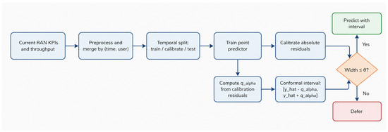
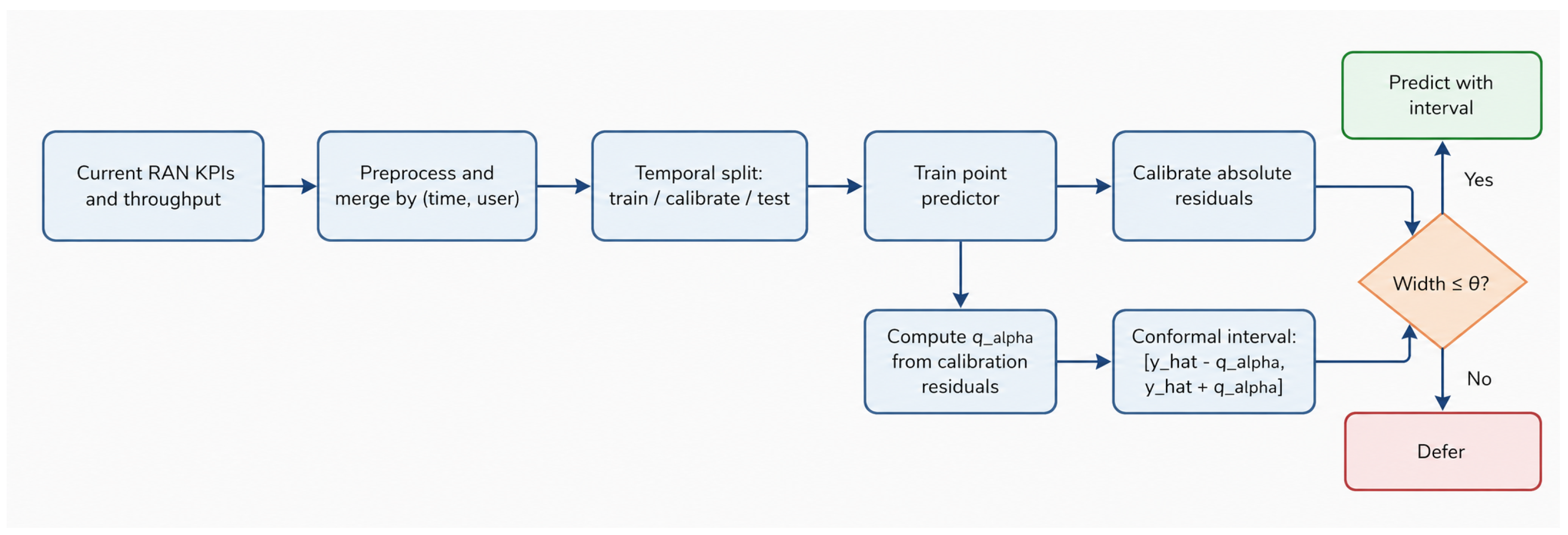
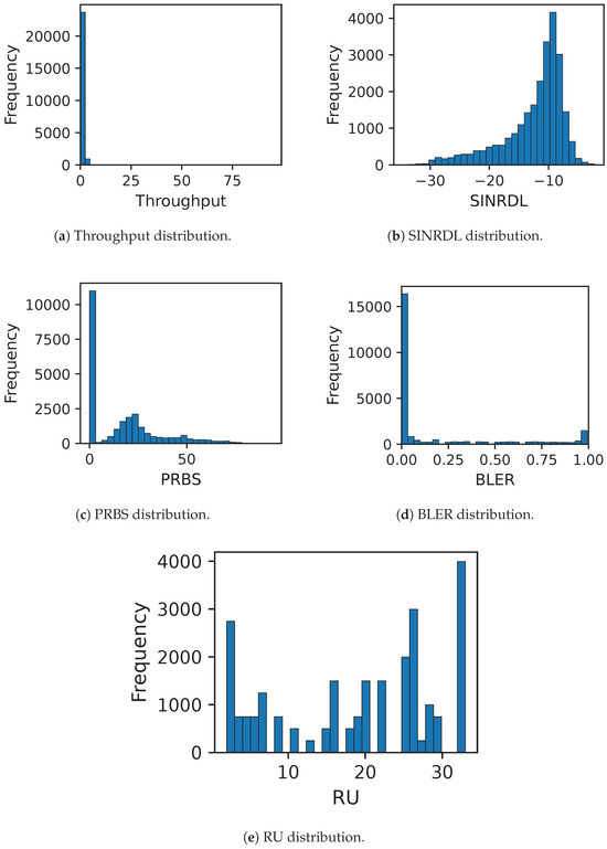
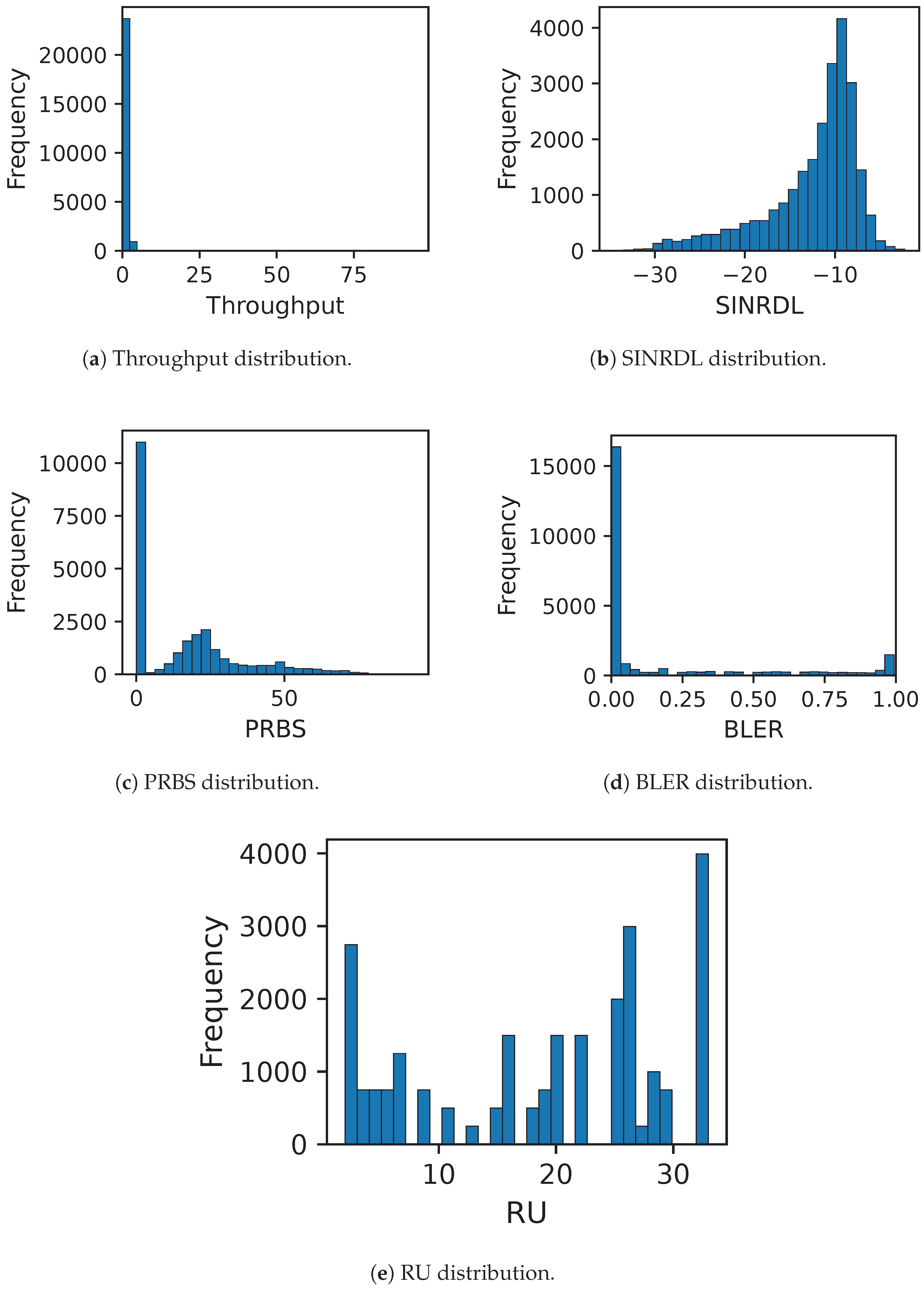
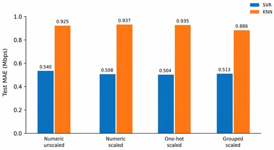
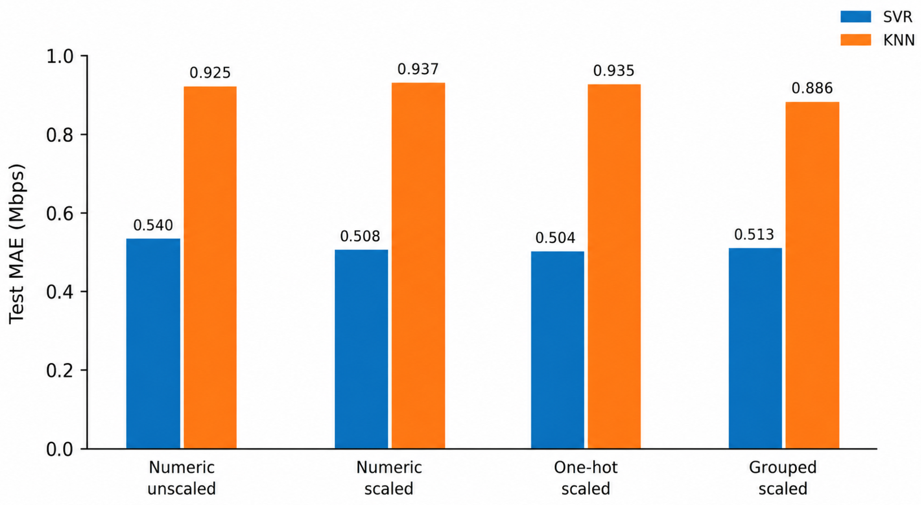
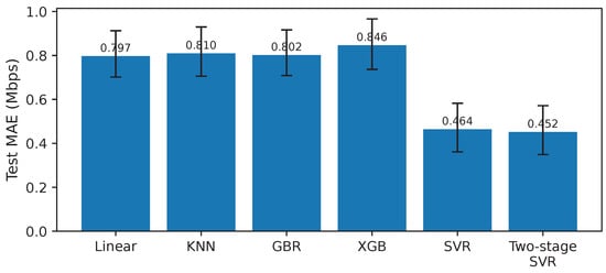
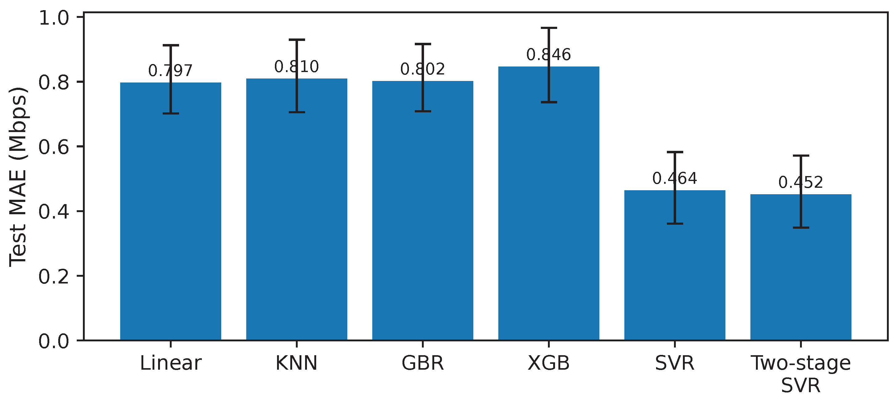
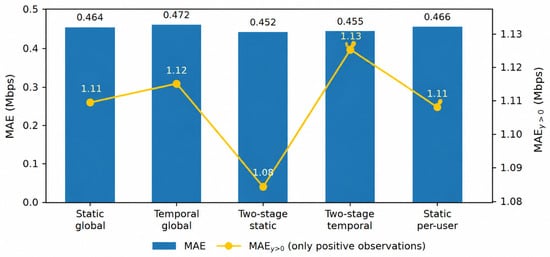
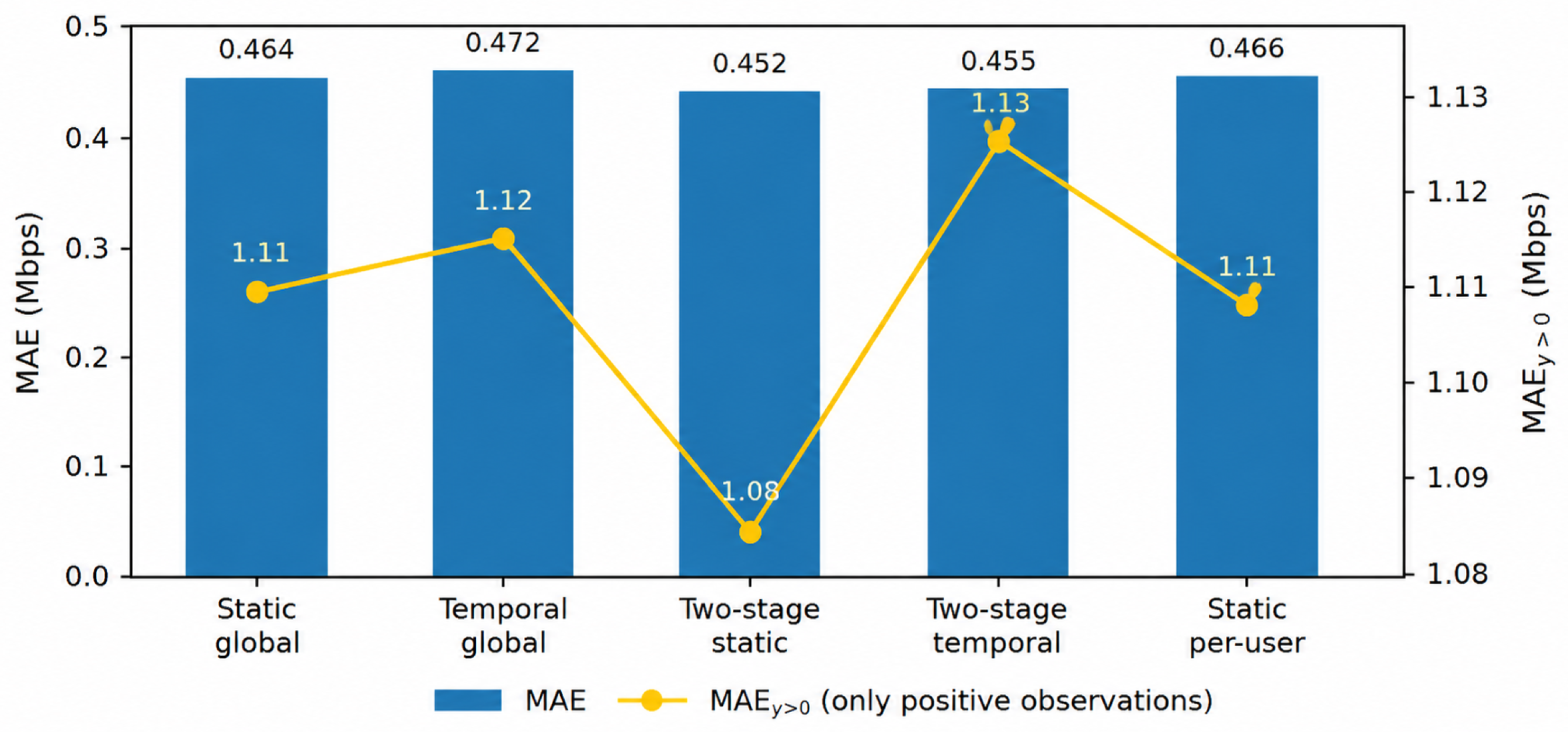
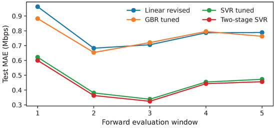
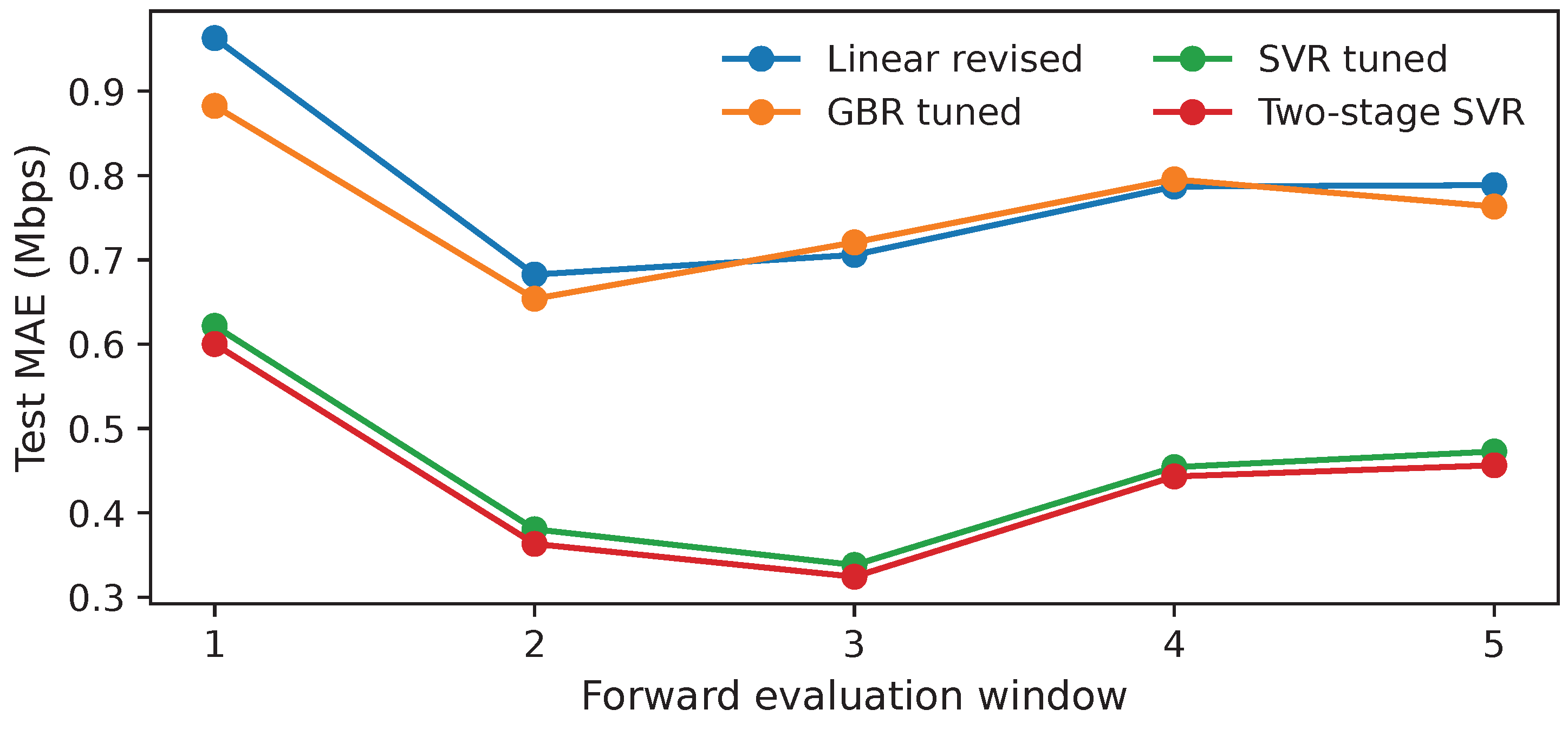
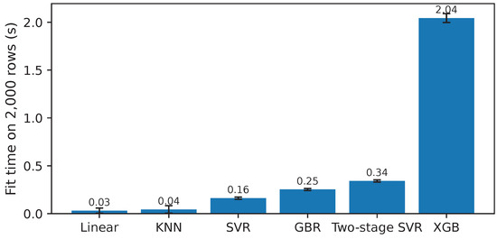
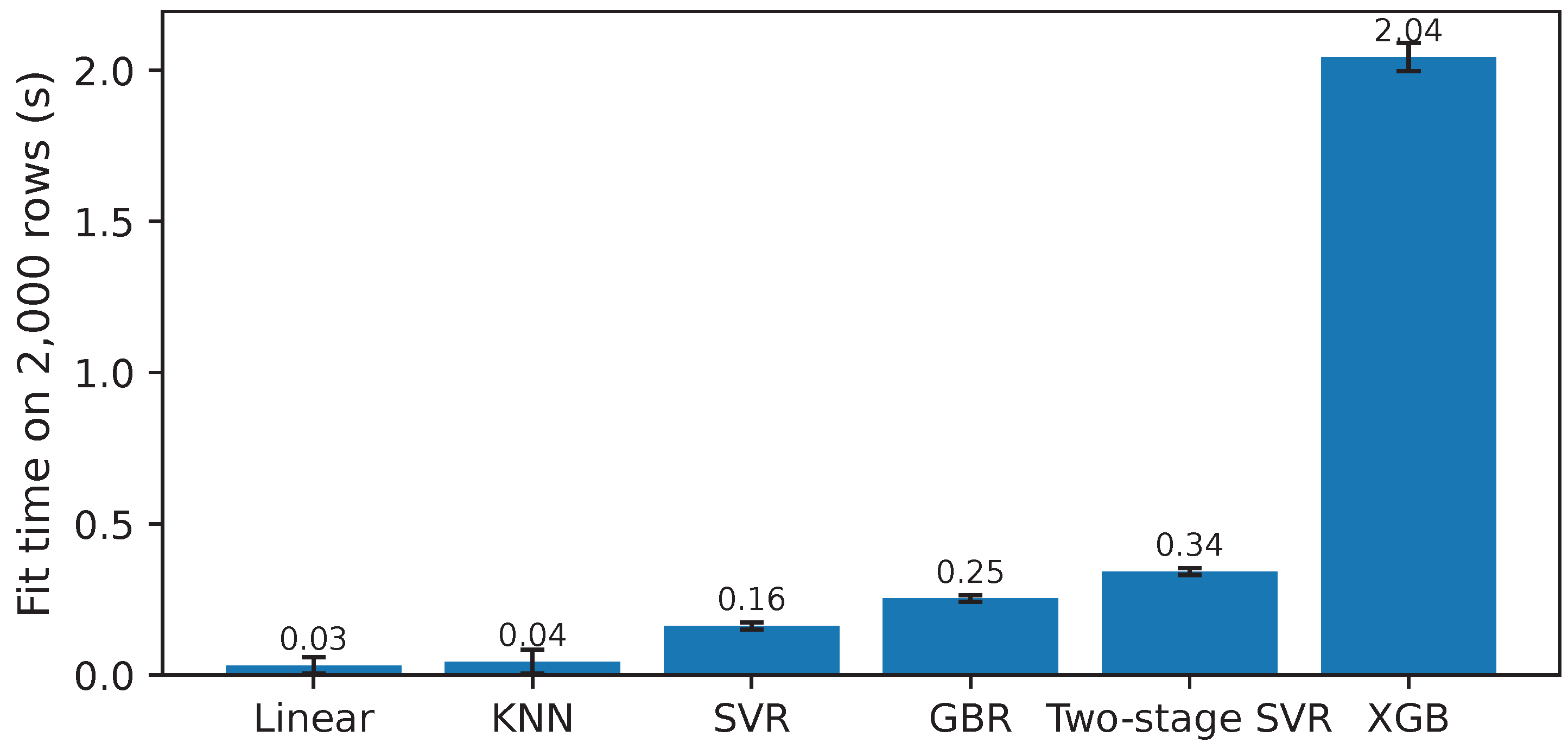
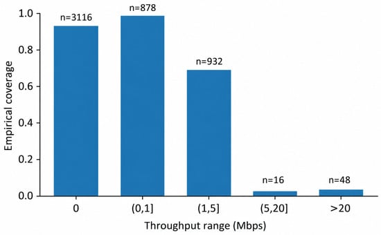
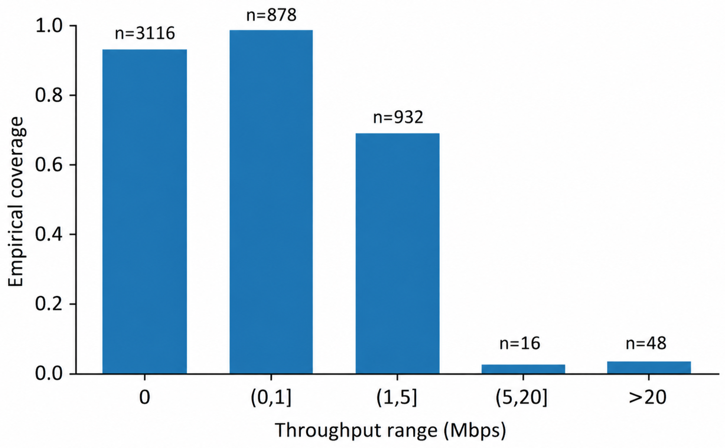
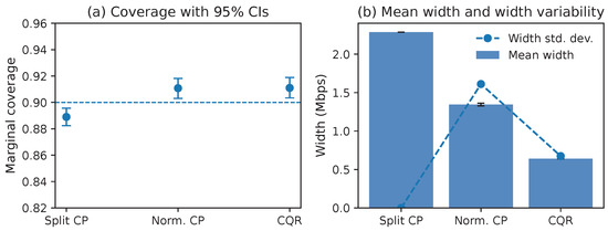
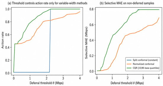
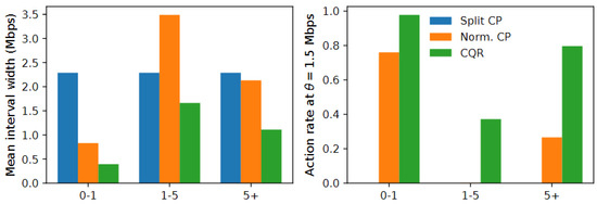
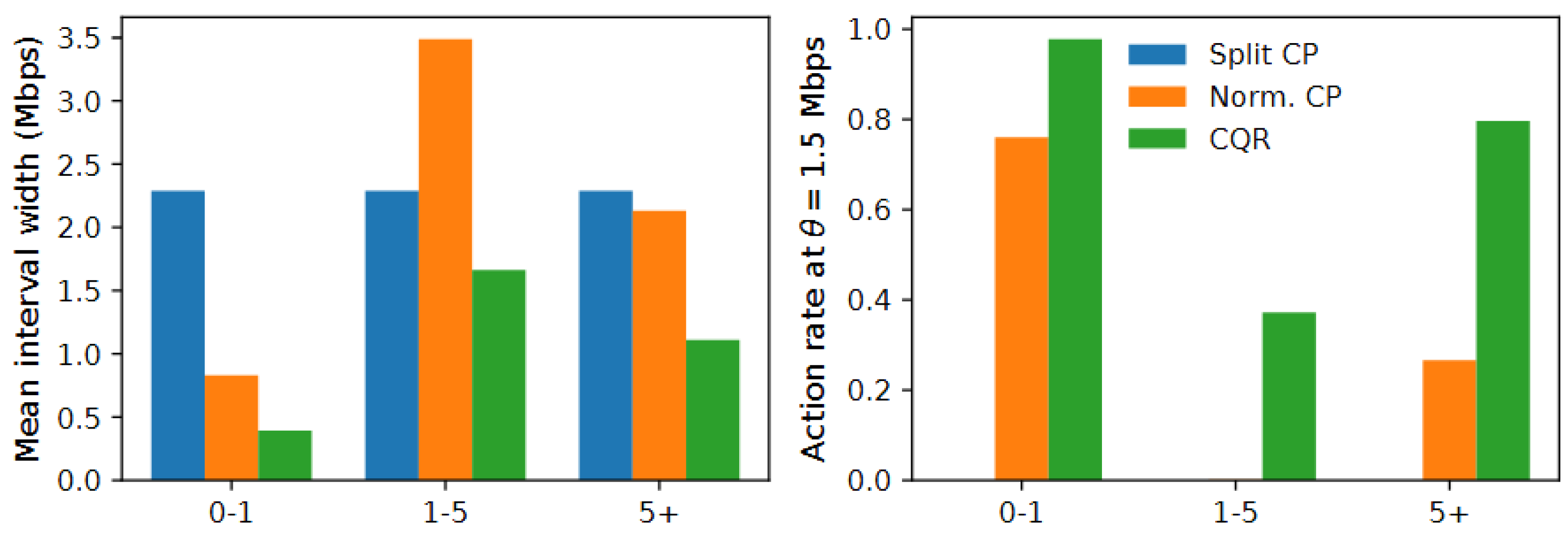
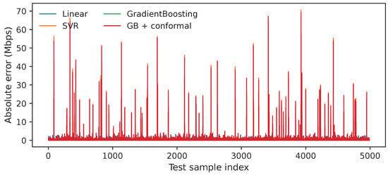
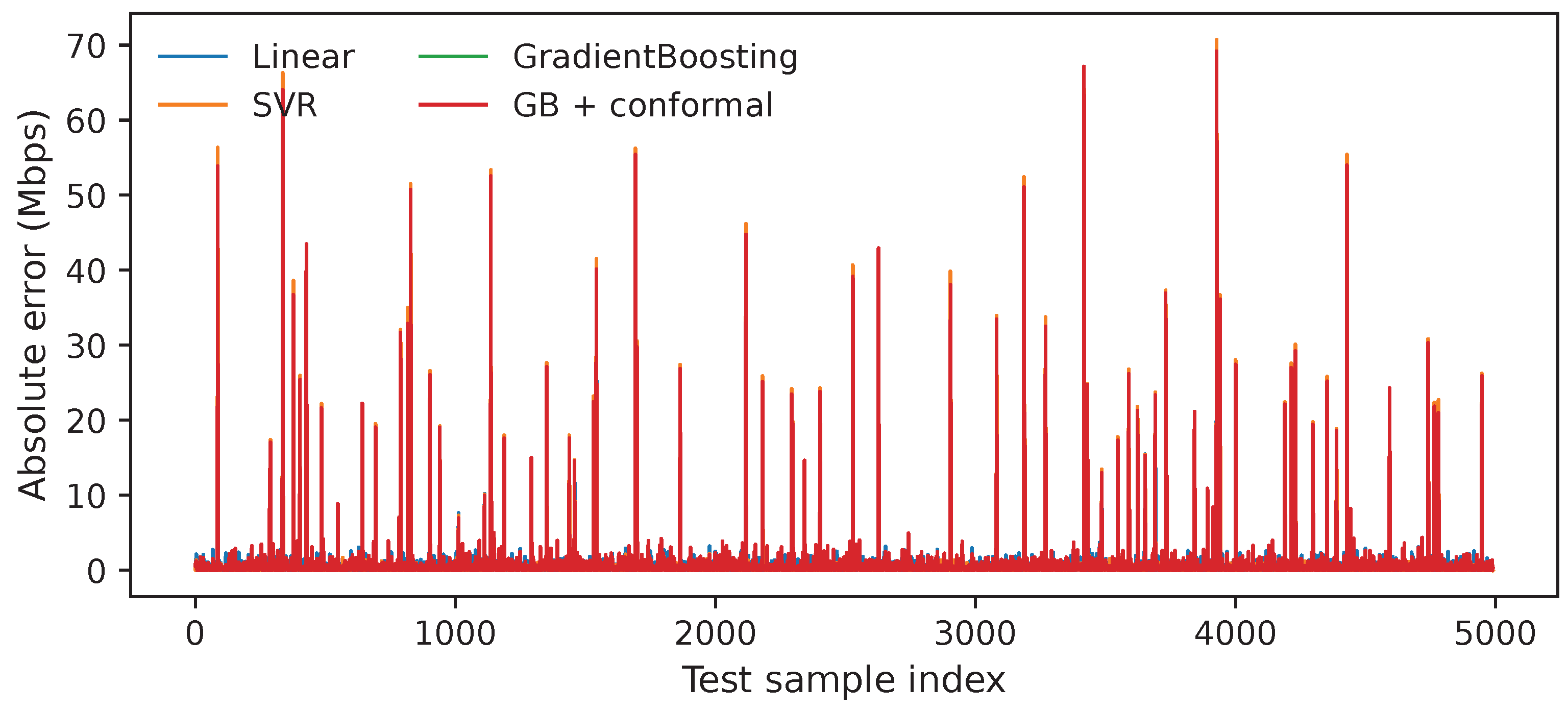
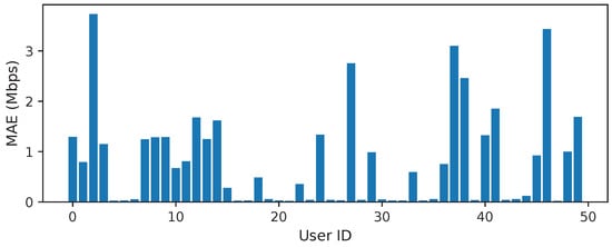
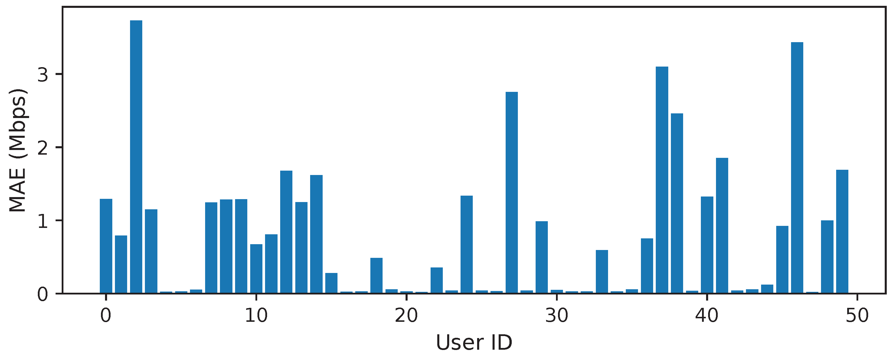
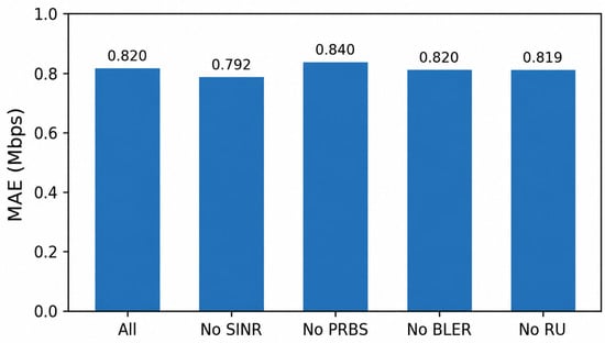
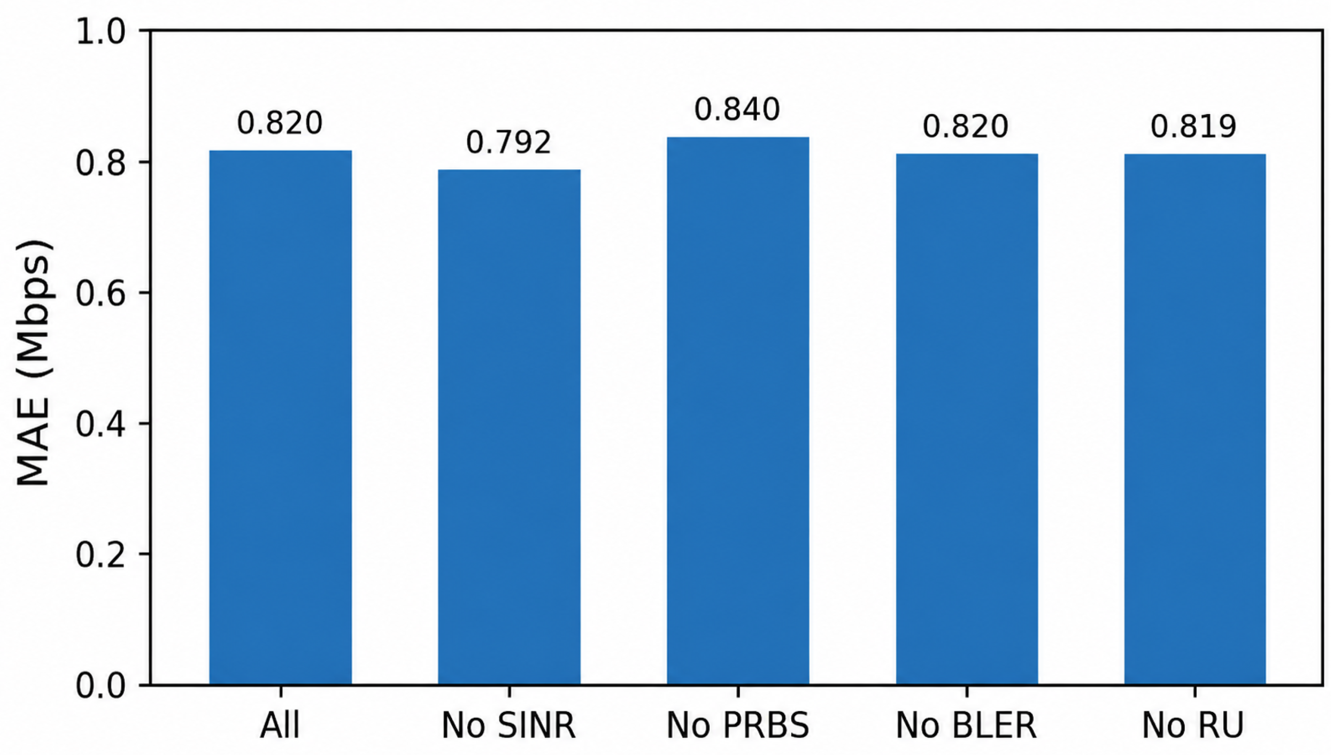
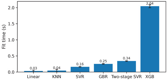
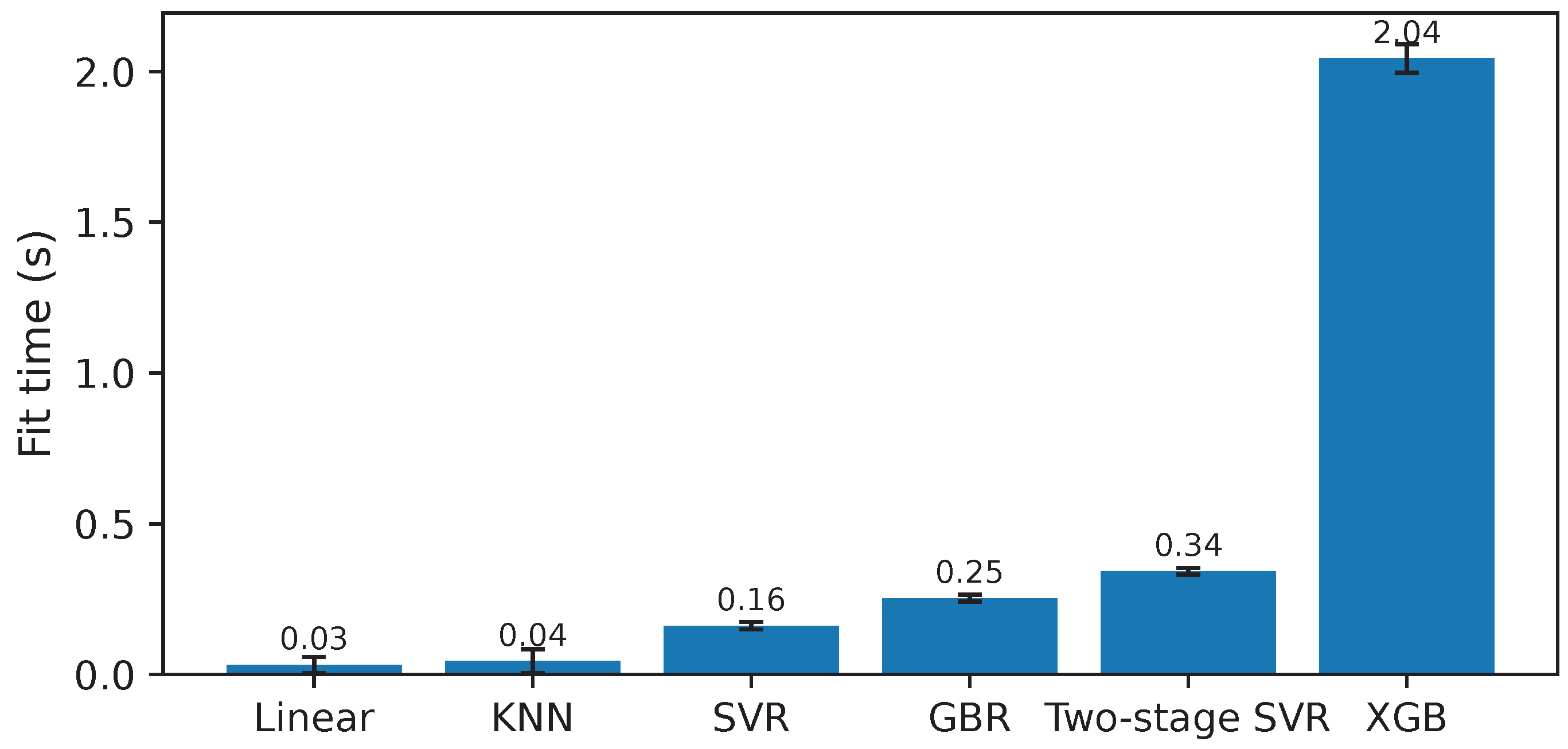
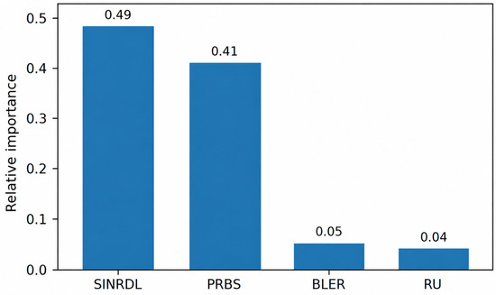
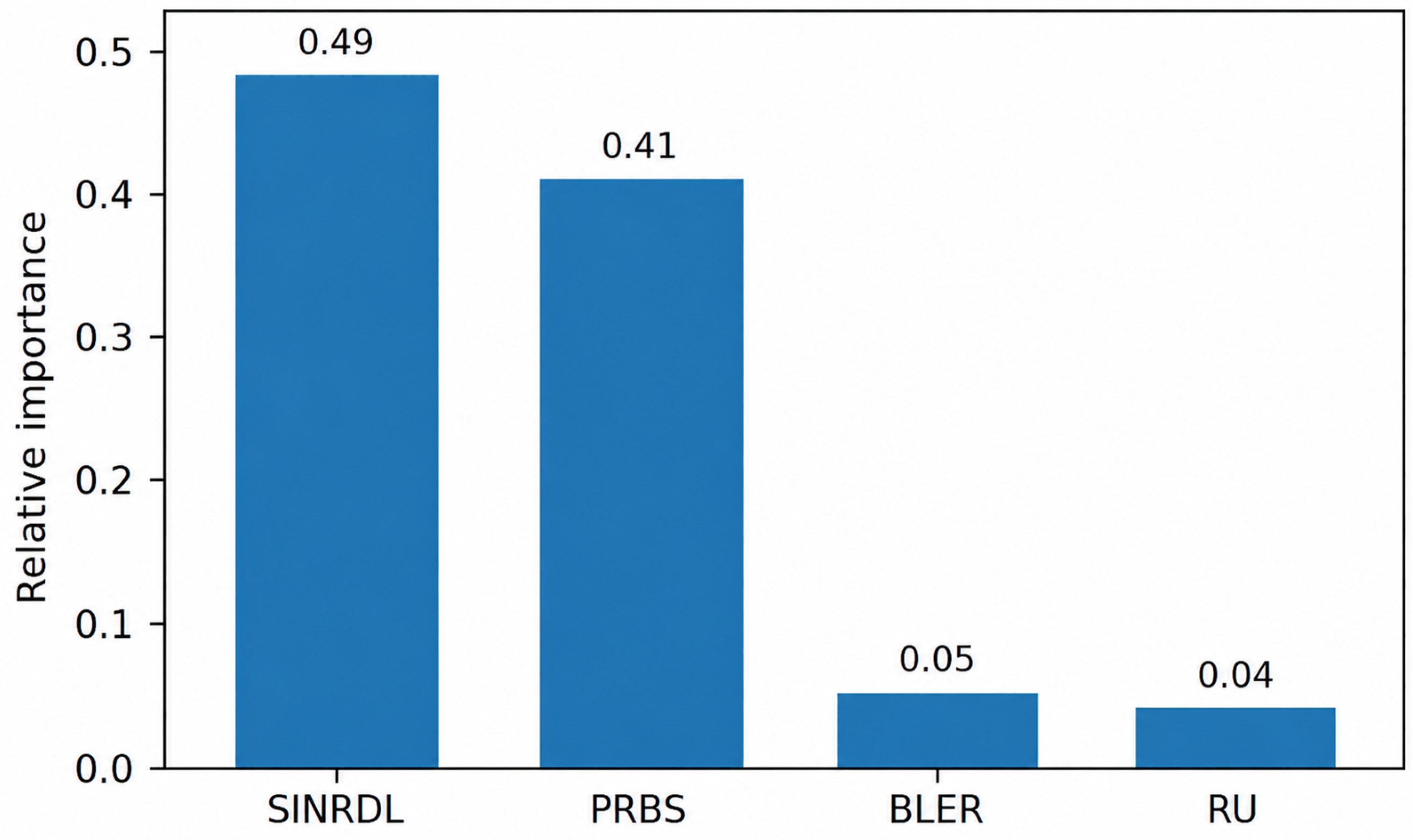
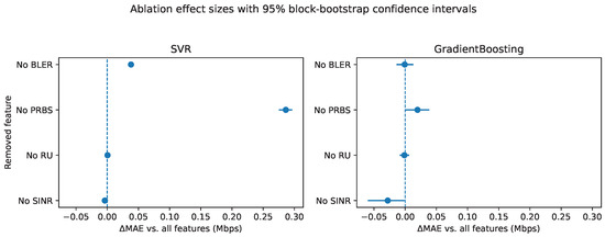

Disclaimer/Publisher’s Note: The statements, opinions and data contained in all publications are solely those of the individual author(s) and contributor(s) and not of MDPI and/or the editor(s). MDPI and/or the editor(s) disclaim responsibility for any injury to people or property resulting from any ideas, methods, instructions or products referred to in the content. |
© 2026 by the authors. Licensee MDPI, Basel, Switzerland. This article is an open access article distributed under the terms and conditions of the Creative Commons Attribution (CC BY) license.