


Abstract
We construct Galois coordinates that connect general three-dimensional shape representations with a layerwise spectral description of convolutional networks. Two spirals on an auxiliary ellipsoid form a closed contour; for q ≡ 3 (mod 4), their nodes are indexed by the quadratic-residue subgroup and its negative coset in the Galois field GF(q). A shape is represented by a radial profile or volumetric cell occupancies, allowing for concavities, cavities, and disconnected components. The contour produces cyclic arrays of length q − 1, while each branch has length (q − 1)/2; roots of unity of both orders exist in the original field. We derive branch-symmetry conditions, explicit spectral mixing for polynomial activations, and unique reconstruction of convolution kernels from prescribed transfer matrices. We also prove covariance of the occupancy representation and convergence under decreasing cell diameters, with a conditional error bound for a spherical carrier. Numerical checks cover 72 shape–resolution combinations and quadrature sensitivity of occupancies and quantized codes. A fixed spectral projector distinguishes centered and displaced cavities in a prescribed family of 84 shapes at two quadrature densities, with exact agreement between direct and spectral calculations. Generalization to real data and hardware efficiency remain untested.
1. Introduction
Abstract algebra has long provided practical tools for information processing, with finite fields supporting error correction and efficient implementations of coding and cryptographic algorithms [1,2]. Recent applications include polynomial-ring methods for post-quantum key establishment and computation on encrypted data [3,4], as well as Clifford-algebra methods for the symmetry-preserving neural processing of geometric fields [5]. These applications motivate exploring finite algebraic structures as a common basis for organizing three-dimensional shape representations and their processing operators.
Abstract-algebraic methods are also used directly in the design of convolutional neural networks: group representations provide a framework for parameterizing symmetry-constrained kernels [6], while Clifford algebras support convolutional and Fourier layers for coupled scalar and vector fields [7]. Polynomial factorization and algebraic geometry are further used to characterize the functions represented by linear and polynomial convolutional networks, quantify their expressive capacity, and analyze critical points arising during training [8,9,10].
The Fourier–Galois transform, or discrete Fourier transform over a finite field, is widely used in information processing, including error-correcting coding and the spectral representation of digital convolutions [1,11,12]. Its number-theoretic forms also support fast polynomial multiplication in modern cryptographic systems, including post-quantum key establishment and computation on encrypted data [3,4].
For many three-dimensional object-recognition tasks, the spatial shape of an object, referred to here as its three-dimensional silhouette, can provide sufficient discriminative information without color or texture [13,14]. Various methods have been developed for identifying such shapes, including point-based multilayer perceptrons, hierarchical geometric networks, vector-valued feature models, mesh transformers, and state-space models [13,14,15,16,17].
For convolutional analysis of three-dimensional objects, associating sampled geometric directions and local features with finite symmetry groups provides a systematic way to express prescribed spatial transformations as permutations of feature indices and to organize convolutional weight sharing [18,19]. Successful applications to point-cloud registration and volumetric image segmentation [20,21,22] demonstrate the practical value of such geometry–algebra correspondences and motivate investigating analogous mappings into finite fields. A coordinate system with a prescribed geometric symmetry offers a convenient way to describe such silhouettes, especially when relatively few points capture their distinguishing features, motivating the spatial compass-rose construction considered below.
Spherical tessellations, including equal-area partitions [23,24], and the placement of reference points on the sphere [25,26] have been investigated in numerous studies, offering diverse finite grids for geometric representations. As these constructions contain finitely many cells or reference points, they provide a setting for exploring different finite algebraic structures, including Galois fields when the grid cardinality and required operations are compatible.
A spatial analog of the compass rose was proposed in [27], associating a finite set of geometric directions with elements of a Galois field or a subgroup of its multiplicative group. The directions are defined by regular and semiregular polyhedra, while the discrete logarithm converts a single algebraic label into partial indices. The construction aligns a geometric alphabet of directions with a finite algebraic structure suitable for encoding and algorithmic processing.
We extend this approach to spatial shape representation and the classification of three-dimensional objects. Once a direction has a discrete label, it can carry a boundary position, a sequence of intersections with the object, or radial-layer occupancies. The alphabet of directions thus becomes the basis of a shape descriptor, referred to below as a shape portrait. Related developments of finite-field coordinate systems are discussed in [28,29].
The coordinate carrier is independent of the object’s surface. The sphere or ellipsoid supporting the reference nodes is an auxiliary surface. The enclosed object may be rounded, elongated, angular, concave, perforated, or composed of separate parts. Matching the number of directions to the field order organizes the data without constraining the object’s geometry.
Different representations of three-dimensional shapes lead to different computational architectures in computer vision. Multi-view classification is considered in [30] and the direct processing of point sets in [31]. Our construction provides a compact representation in a prescribed set of spatial directions organized through finite-field algebra. It can supply an ordinary classifier or a specialized network whose linear part uses finite-field arithmetic.
Here, a three-dimensional silhouette means the object’s spatial shape, represented by a segmented set and its boundary, without texture or color. This usage differs from the two-dimensional silhouette in an individual image. The input is a three-dimensional mask, a geometric model, or a spatial envelope recoverable from several views. The coordinates organize the available shape information; the data source determines its completeness.
Spherical shape representations and orientation-independent descriptors have a substantial history, including spherical-harmonic descriptors [32]. Membership functions are also used in modern implicit representations such as Occupancy Networks [33]. Neither radial description nor occupancy alone constitutes a new result here. We investigate their alignment with a specific two-branch grid and the finite-field organization of processing operators.
The spectral framework builds on [12,34]. Partial convolutions and integer reduction to a prescribed discrete scale are studied in [34]. Compatible finite-field bases provide analogs of transfer functions for partial digital convolutions in [12]. We connect these tools to three-dimensional shapes: the coordinate construction supplies one-dimensional cyclic arrays whose periods match the orders of roots of unity in the original field.
Our aim is to connect the spatial portrait to the spectral description of convolutional processing. Traversing both spirals gives period q − 1, and each branch has period (q − 1)/2. Both transforms exist without a further field extension at the selected field order. The linear parts of networks built from these cyclic convolutional layers are therefore described by transfer matrices. Activations enter the exact layerwise spectral representation as separate operators. Prescribing the spectral matrices also permits reconstruction of the kernels and formulation of a synthesis problem.
The constructive contribution is the joint organization of a general shape representation, a closed traversal, compatible finite-field periods, and processing operators. The convolution theorem supplies the algebraic tool. We extend the directional construction in [27] with volumetric cells and explicit compatibility conditions between geometric branch exchange and spectral operators in both the paired and contour representations. For a spherical carrier, we give a conditional volume-error bound in terms of angular and radial resolution and distinguish geometric, integration, and quantization errors. An explicit formula describes polynomial activation in the spectral domain. A complete numerical example connects cavity portraits to a fixed projector and readout, with checks of quadrature sensitivity and integer implementation.
In this work, we propose a shape-dependent occupancy portrait on a fixed paired geometric carrier, combining compatible finite-field Fourier processing, explicit branch symmetries, and volumetric reconstruction. Tests on synthetic shapes verify the representation and operator identities, while gains in classification accuracy and computational efficiency remain to be demonstrated.
2. Materials and Methods
2.1. Geometric Carrier of the Double Spiral
2.1.1. Ellipsoid of Revolution and Equal-Area Coordinate
Consider an auxiliary prolate ellipsoid of revolution with equatorial semiaxis a and longitudinal semiaxis c > a:
The spherical case is obtained at c = a. A prolate carrier is convenient for objects with a distinguished longitudinal direction, but its aspect ratio is fixed across the classification task. Fitting each object through independent axis scaling could remove proportions needed to distinguish classes.
Set u = z/c, with −1 ≤ u ≤ 1. The radius of a parallel and the surface-area element are
Define the normalized surface area from the south pole to level u by
The function U is strictly increasing, satisfies U(−1) = 0 and U(1) = 1, and has inverse u = u(U). Equal increments in U correspond to equal-area bands. We use z(U) = cu(U) and .
Evaluation of the equal-area inverse. The numerator integral in (3) has an elementary antiderivative. , where ∆ = c2 − a2 > 0. Since F(−1) = −F(1), Equation (3) becomes . Given U, the corresponding u is the unique solution of F(u) = (2U − 1)F(1); strict monotonicity permits a safeguarded scalar root solver, such as bisection. Although the integral has this closed elementary expression, an elementary closed-form inverse is not obtained for a general prolate ellipsoid.
In the spherical limit c = a, the area factor is constant, and ; hence u(U) = 2U − 1. The numerical inversion is performed once when constructing a fixed grid and is not repeated for every input shape.
Uniformity in ellipsoidal surface area differs from uniformity in solid angle. Directional coverage must therefore be assessed separately using unit vectors from the center to the nodes. These criteria coincide for a sphere. Spiral point distributions on a sphere have been studied, for example, in [26]; here, the equal-area coordinate organizes paired nodes on an ellipsoid.
2.1.2. Two Paired Branches
For a prescribed monotone azimuthal law Φ(U), define
Meaning of the azimuthal law. Φ(U) specifies how the reference direction rotates around the longitudinal axis as the equal-area coordinate increases from the south pole (U = 0) to the north pole (U = 1). It is fixed before processing any object and is not an object-dependent fit. In the grid used in this article, Equation (6) makes this choice explicit: with the golden angle ; consequently, for . Both branches use the same Φ and differ by exactly π in azimuth.
At the same U, the points have the same height and are exchanged by a rotation through π about the longitudinal axis. The branches are disjoint for 0 < U < 1 and meet at the poles. Traversing the first branch from south to north and the second in reverse produces a closed path. The paired nodes are generally not antipodal about the center because the rotation preserves z.
Here “meet at the poles” concerns the continuous parameterized curves, not coinciding sampled nodes: at U = 0 or U = 1, the parallel radius ρ(U) vanishes, so both azimuths represent the same pole. Every discrete level Uj lies strictly between 0 and 1; thus, and are distinct for all sampled node pairs. The opposite azimuths are a half-turn about the z-axis, not central inversion of the entire point.
Place n nodes on each branch. A convenient initial construction uses the golden angle :
At the nodes, Φ(Uj) = jγ. Write . Each equal-area band contains a pair of nodes, and the azimuth changes by the golden angle between consecutive bands. The discrete sample excludes the poles, preventing coincidence between the two branches.
This is a constructive initial grid; optimality in minimum angular separation is not assumed. Nodes may be refined while preserving the exact pairing. The geometry is fixed before training and shared by all objects. Figure 1 illustrates the spherical and prolate cases.
Figure 1.
Two-branch grids in the Galois field GF(59) for c/a = 1 and c/a = 2. Colors identify branches H and −H; segments show three node pairs with the same partial index. Each pair is related by rotation about the z-axis, rather than central inversion. Variations in marker brightness are due to depth shading in the 3D visualization and do not represent additional information.
2.2. Algebraic Indexing of the Two Branches
2.2.1. Partition of the Multiplicative Group
Let q = pm be an odd prime power.
Why q and q − 1 appear. GF(q) has exactly q field elements, but the spatial labels are drawn only from its nonzero multiplicative group GF(q)×, which has q − 1 elements. We therefore set q − 1 = 2n to match the 2n geometric nodes (n points on each branch). The excluded zero may be reserved for a separate center value but is not a third spatial branch. For q ≡ 3 (mod 4), n = (q − 1)/2 is odd, which allows for the particular two-coset decomposition used below.
Standard properties of finite fields and their multiplicative groups are given in [35]. To obtain a canonical correspondence with the two branches, we require
The subgroup of quadratic residues has order n:
Under (8), −1 is not a square. Consequently,
The additional condition q ≡ 3 (mod 4) ensures that −1 is not a quadratic residue. Thus H and −H have no common element, and their union is all of GF(q)×; this provides two distinct, equally sized branches. The condition is not needed merely to define cyclic convolution, but it is used for the specific branch labeling and involution in this manuscript.
Let g be a primitive field element and h = g2. Then h has order n and generates H. Define a bijection between the nodes and algebraic labels:
Each nonzero field element labels exactly one node. Zero is not assigned a spatial direction; a central state can be stored separately if needed.
2.2.2. Partial Indices and Geometric Interpretation
Each label has a unique representation
Here, b identifies the branch and j the node position. For e = loggα modulo 2n,
Because n is odd, the parity of e determines the branch. The expression (e − bn)/2 then determines j modulo n. This extends the use of the discrete logarithm to extract partial coordinates [27]. For a fixed small field, label–index conversions can be tabulated.
Introduce
Operation J corresponds exactly to rotation of the auxiliary surface through π about the longitudinal axis. Operation T cyclically permutes indices on each branch. It is generally not a rigid spatial rotation because both height and azimuth change. In particular, the wraparound from j = n − 1 to j = 0 connects regions near different poles. Algebraic periodicity and Euclidean proximity must therefore be treated separately.
Interpretation of the two index operators is as follows: In Equation (14), J denotes multiplication of a field label by −1 and therefore swaps paired branch nodes while leaving the partial position j unchanged. T denotes multiplication by h: if α = (−1)bhj, then Tα = (−1)bhj+1, with j taken modulo n. The cyclic step T stays on the same branch, but generally, it is not a short physical movement along the surface. This separation between exact algebraic shifts and geometric distance is essential when interpreting a cyclic convolution.
Proposition 1.
Uniqueness of partial indices. Under (7) and (8), the map
is a group isomorphism and defines a bijection with the nodes of the two branches.
Proof.
The orders of h and −1 are n and 2. Since n is odd, −1 ∉ H, so H and −H are disjoint. Within each coset, powers of h uniquely determine an index modulo n. Thus, Ψ is injective and covers all 2n nonzero elements. Label multiplication adds the partial indices in their respective cyclic groups, preserving the group operation. Distinct spatial nodes follow from distinct Uj within each branch and opposite azimuths for paired nodes with ρ(Uj) ≠ 0. □
Further detail for Proposition 1. Because GF(q)× is cyclic of order 2n, a primitive element g generates all nonzero labels and h = g2 has order n. Its powers give n distinct elements of H. Since n is odd and −1 ∉ H, the other n nonzero elements are precisely −H; hence each α has a unique expression α = (−1)bhj with b ∈ {0, 1} and . Multiplication gives , so the two partial indices add modulo 2 and n, respectively. This proves both uniqueness and preservation of the group law. The final association with the geometric nodes uses their previously defined one-to-one ordering and is not a claim that field addition represents a spatial displacement.
The isomorphism concerns the multiplicative group. It assigns no geometric interpretation to field addition. This distinction matters when comparing finite-field processing with the ordinary processing of two arrays.
2.2.3. Example in GF 59
For the prime field GF(59), N = 58 and n = 29. The element g = 2 has order 58, while h = 4 has order 29. The branch labels are
The grid consists of two branches with 29 nodes each. Exchanging paired nodes changes the label’s sign, and the cyclic algebraic shift multiplies it by 4. The spatial portrait becomes two equal-length sequences connected by an exact geometric involution.
2.3. Representation of General Three-Dimensional Shape
2.3.1. Object Normalization and Radial Coordinate
Let the input object be a bounded measurable set . Choose a center o, an orthogonal orientation matrix R, and one positive scale s. Define
Choose the scale so that K lies inside the carrier (1); such a scale exists for every bounded object. The center can be determined from a geometric model or segmented mask and need not belong to the object. Training and inference use the same normalization rules. If absolute size helps distinguish classes, retain s as an additional feature.
For each node, define its unit direction and radial path:
The function P connects finite-field labels to Euclidean geometry. The normalized radial coordinate t corresponds to distance t‖P(α)‖ from the center. Arithmetic differences between labels do not determine distances or angles.
2.3.2. Radial Profiles of Star-Shaped Objects
If K is closed and star-shaped about the origin, its intersection with each radial path is an initial segment. One number describes the shape in that direction:
Membership along the selected direction is determined by 0 ≤ t ≤ r(α). This compact portrait contains q − 1 radial values. It is useful when the relevant objects are star-shaped or deviations from this property do not affect recognition.
For a general shape, the last boundary intersection does not specify all intervening segments. A path can intersect two disconnected parts or pass through a hole. Replacing this structure with one outer radius fills the gaps and removes features. General three-dimensional objects therefore require a more complete representation.
2.3.3. Occupancy Functions and Radial Layers
Introduce the object’s indicator:
Its restriction to a radial path is
This definition does not require convexity, star-shapedness, or connectivity. For geometric models with finitely many boundary intersections on each path, the occupied radial segments can additionally be written as
Indicator (20) remains the general definition and does not require finitely many intervals. Discretizing t gives a multilayer occupancy portrait.
Spatial cells provide a more stable sampling scheme than values on isolated paths. Let Vα be the angular Voronoi cell on the unit sphere for direction v(α). In any unit direction v, the ellipsoid boundary has radius
Derivation of (23) is as follows: A ray from the origin with unit direction v = (vx, vy, vz) has points x = rvx, y = rvy and z = rvz. Substitution into (1) gives . Solving for its unique positive intersection with the carrier boundary yields RE(v) as stated in (23). Therefore, multiplying the normalized radial level t by RE(v) maps every angular direction to the corresponding interior point of the ellipsoid.
Partition the radial coordinate by 0 = t0 < t1 < ⋯ < tL = 1, and define
Include the outer boundary in the last layer. These cells cover the carrier volume up to partition boundaries. The occupancy fraction is
Every part of the object belongs to a cell, including regions between reference directions. For a surface without a specified enclosed volume, (25) can be replaced with a cell–surface intersection indicator or surface-area fraction under a fixed rule. The spatial partition provides geometric applicability; cell dimensions determine which small features remain distinguishable.
2.3.4. Shape Information Available from Vision Data
The portrait can be computed from a segmented three-dimensional mask, a closed polygonal model, or surface data after defining its interior. A point cloud alone does not determine occupied volume without additional assumptions. It requires a surface-based variant or a consistent reconstructed geometric model.
If only two-dimensional silhouettes from several views are available, their spatial envelope contains only features recoverable from those observations. The visual-hull concept describes this limitation [36]. Galois coordinates do not reveal unobserved recesses or internal cavities. In that setting, classification concerns the observed envelope, and the acquisition method determines the completeness of information about the actual shape.
2.3.5. Covariance of the Volumetric Portrait
Let Jz denote the Euclidean rotation (x,y,z) ↦ (−x,−y,z). Consider a fixed center, scale, and axis system. The following statement does not include independent re-estimation of principal axes after rotation.
Proposition 2.
If all directions share the same radial levels, then
Proof.
Equations (4) and (5) give v(−α) = Jzv(α). Rotation preserves angular distance, so Vα maps to V−α up to boundaries. The ellipsoid of revolution and radial levels are also preserved, giving . Applying the volume-preserving rotation to the numerator and denominator of (25) yields (26). □
This is an exact symmetry of the geometric partition. The cyclic index shift T does not, in general, define an isometry of its spatial cells.
2.3.6. Convergence Under Partition Refinement
Let E be the closed volume inside (1), and let be a sequence of finite partitions of E by cells of the form (24). Here, s indexes partitions and is distinct from the scale in (17). Define the piecewise constant reconstruction
Proposition 3.
For every measurable K ⊂ E, if , then
Proof.
Let Ps denote cell averaging. It is a contraction in L1(E) because the integral of the absolute cell average cannot exceed the integral of the absolute input. For every ε > 0, choose a continuous f on E with , using density of continuous functions in L1 on a bounded volume. Then ‖χK − PsχK‖1 ≤ 2ε + ‖f − Psf‖1. The last term is at most Vol(E)ωf(ηs), where ωf is the modulus of continuity. Uniform continuity of f and arbitrary ε establish (28). □
The decrease in maximum diameter is essential. For a fixed carrier, it can be ensured by reducing the angular covering radius and the maximum radial step. Increasing q alone, without checking coverage, does not prove convergence of the selected spiral sequence. We evaluate coverage for four specific grids; asymptotic optimality of their node placement is not claimed.
For a unit spherical carrier, the resolution dependence can be quantified. Let δs be the angular covering radius and , with δs ≤ π/2. Two directions in one Voronoi cell are separated by at most 2δs, so
Additionally assume that the object’s boundary admits constants BK and η0 > 0 such that Vol{x ∈ E: dist(x, ∂K) ≤ η} ≤ BKη for 0 < η ≤ η0. For ηs ≤ η0,
Indeed, the error integral on a cell C with exact occupancy wC is 2wC(1 − wC)Vol(C) ≤ Vol(C)/2. Fully occupied and empty cells contribute zero. Every partially occupied cell lies in the ηs neighborhood of the boundary; summation gives (30). This bound requires the stated boundary condition and does not prescribe the decrease in δs with q for the selected spiral. Proposition 3 remains valid for general measurable objects without a rate estimate.
Round (25) to the nearest of q levels, and apply Q. Decode each field value as , since itself returns the integer level index. The resulting reconstruction satisfies
This follows by bounding each level’s rounding error and summing cell volumes. The bound concerns decoded occupancy levels and does not impose an order on field elements. Equations (28)–(31) separate geometric information loss from additional quantization error. Convergence does not imply exact recovery of every object on one finite grid. The L1 norm describes volume and cannot distinguish sets differing only on a zero-volume set. Topology preservation and Hausdorff convergence of boundaries require additional assumptions; the surface-based representation requires a separate estimate.
If exact averages are replaced with numerical values , let denote their quantized and decoded reconstruction. Set , and define εQ,num(K) analogously. The triangle inequality gives
The terms describe geometric discretization, occupancy integration, and quantization. Comparing two quadratures measures numerical sensitivity; without a further estimate, it does not bound deviation from the exact wC. Occupancy and code stability must therefore be checked separately from the change in total reconstruction error.
2.4. Multichannel Shape Portrait
2.4.1. Geometric Features and Finite-Field Encoding
Fix a quantizer Q for finite-field processing. In a prime field, a level can be encoded directly as an integer from 0 to q − 1. For GF(pm) with m > 1, specify a bijection ιq between these level indices and field elements, consistent with the chosen field basis:
The function GK is defined on GF(q)× × {1, …, L} and contains L(q − 1) field elements. The layer index is a separate finite index and need not belong to the same field. Binary occupancy uses only 0 and 1. If processing does not use field arithmetic, wK can be stored in real or fixed-point format, with only the direction labels organized algebraically.
These modes must be distinguished. Field indexing organizes spatial data, whereas field encoding specifies the feature arithmetic. Encoding an ordinary level as a field element does not make modular operations preserve the order of levels or automatically reproduce numerical convolution.
2.4.2. Branch Representation and Data Size
For each radial layer, define two channels:
The resulting array has 2L channels of length n; at L = 2, it has four channels. Its input size is known in advance, which is useful for a specialized classifier. A complete array requires the corresponding source geometry. Partial visibility requires a separate validity mask; unknown occupancy must not be treated as zero.
Table 1 gives the payload for GF(59) with dense bit packing. It excludes normalization parameters, validity masks, the classifier, and auxiliary information.
Table 1.
Shape-representation payload for 58 directions.
The size 2L × n depends on representation resolution rather than the vertex count of the input mesh, allowing for a predetermined input-buffer size. Reducing the buffer loses geometric details; q and the layer count must be chosen according to the distinctions between target classes.
2.4.3. Comparison with Ordinary Indexing
Fix the same directions, radial levels, quantizer, and object. An ordinary portrait is related to the field portrait by . Proposition 1 makes this a reversible relabeling of array entries. Values, geometric distinguishability, and the number of stored levels coincide exactly. If the grid is known, neither representation requires a separate stored label for each node.
The payloads in Table 1 are therefore also achievable by ordinary integer encoding of the same q levels. Field indexing alone provides neither independent memory savings nor greater geometric accuracy. Its role is a unified description of partial indices, branch exchange, and spectral operators. Field arithmetic is a separate modeling choice: it provides exact operations in the selected finite structure but changes the meaning of feature addition and multiplication. Its practical efficiency must be compared with arithmetic of the same bit width, including encoding and decoding costs.
For a fixed grid and node ordering, ordinary array indices and Galois-field labels yield the same cell occupancies and descriptor size. Practical differences can arise from the subsequent choice of feature arithmetic, branch-symmetry constraints, and processing operators. A controlled comparison should therefore distinguish relabeling alone, ordinary versus finite-field arithmetic at matched model capacity, and direct versus spectral implementations of the same cyclic operator. To make these distinctions explicit, the following subsection presents a step-by-step algorithm that separates geometric sampling, algebraic indexing, feature encoding, and spectral processing.
2.4.4. End-to-End Algorithm for a Shape Portrait and Spectral Layer
The following algorithm summarizes the complete computational pipeline, from three-dimensional shape normalization and occupancy sampling to Galois-field indexing and spectral processing. The procedure is intended to illustrate the mathematical construction and does not assume a trained classifier in the numerical experiments.
Algorithm 1 (implementation outline; no trained classifier is assumed in the experiments).
| Algorithm 1. Construction of a Galois-Coordinate Shape Portrait and Spectral Processing. |
| Step 1—Input and normalization. Obtain a watertight mesh or segmented 3D mask, define its enclosed set K, and apply a common center, orientation, and scale using (17). A point cloud requires an explicitly chosen reconstruction or surface-only variant. Step 2—Fixed carrier and nodes. Choose the ellipsoid (a,c), field order q ≡ 3 (mod 4), n = (q − 1)/2, and radial levels t0, …, t_L; generate Uj and the paired nodes , from (3)–(6). Step 3—Geometric sampling. Construct the angular Voronoi cells Vα, intersect them with the radial layers to obtain Cαl, and evaluate occupancy fractions from (23)–(25). Step 4—Algebraic indexing. Choose the primitive element g, put h = g2, and associate each node (b, j) with α = (−1)bhj; this step permutes addresses but does not change the measured occupancies. Step 5—Feature encoding. Quantize occupancies to prescribed levels and, only if field arithmetic is selected, encode levels consistently as GF(q) elements. Keep any invalid or unobserved cells separate from genuine zero occupancy. Step 6—Network input. Either form paired length-n channels using (34), or reorder the same values into the length-(q − 1) closed contour using (46). The order must be kept identical during kernel application and reconstruction. Step 7—Spectral processing. Apply a specified cyclic convolution directly or via its finite-field transform and transfer matrices, then apply an explicitly defined activation and inverse transform when required. Step 8—Decision and evaluation. Aggregate the output into a class score or prescribed statistic. Section 3.4 uses a fixed analytic rule without training; a genuine classification benchmark must fit model parameters on training data and evaluate an independent test set. Pipeline summary: 3D mesh/mask → normalization → paired equal-area directions → volumetric cells → occupancies → finite-field labels and optional encoding → cyclic channels → convolution/finite-field spectrum → activation/readout. |
2.5. Convolutional Processing and Branch Symmetry
2.5.1. Weight Sharing
In the simplest setting, channels (34) enter a one-dimensional multichannel network. Write the linear part of a cyclic layer as
The index d enumerates output features, and j − r is taken modulo n. Restricting the kernel support to a small set of shifts gives a compact layer with shared weights. Sums and products in (35) use GF(q) for field processing and the selected numerical format for ordinary processing.
Cyclic convolution uses index regularity to process a sequence along the prescribed traversal. It does not automatically define a local filter of three-dimensional shape. With the golden angle, even consecutive internal indices have large azimuthal jumps, so removing only the branch wraparound does not resolve spatial nonlocality. Section 3.2 quantifies this property.
Local geometric features require neighborhoods based on angular distances between v(α) and processing on the resulting graph. Such a graph can respect J because branch exchange preserves pairwise angular distances. Cyclic spectral processing remains valid for operators intentionally defined on the index sequences. A general local graph operator need not have the spectral form (42).
The exact branch exchange is J. Tying the weights through
makes the linear layer equivariant to this exchange. Applying the same nonlinearity to paired channels preserves equivariance. This follows the principle of group-equivariant networks [37]. Here, the exact geometric symmetry is restricted to the particular rotation represented by J.
2.5.2. Symmetric and Antisymmetric Components
In odd characteristic, 2 is invertible. Transform the channels as
Branch exchange leaves the symmetric channel unchanged and changes the sign of the antisymmetric channel. The transformation is invertible: , and . In GF(59), 2−1 = 30.
The symmetric channel extracts the information shared by paired directions. Using it alone can merge distinct shapes and remove relevant asymmetry. If a class is invariant under branch exchange, both components can be retained during equivariant processing, with invariance imposed at aggregation. Ordinary numerical processing uses the analogous mean and half-difference, interpreted in its own arithmetic.
2.6. Spectral Processing in the Finite Field
2.6.1. Transform on Each Branch
The element h has order n and is a root of unity for a length-n transform in the original field. For a sequence X(j) ∈ GF(q), define the finite-field discrete Fourier transform (DFT) by
Its inverse is
Invertibility follows from
Here, δjr is the Kronecker delta, equal to 1 for j = r and 0 otherwise. The characteristic p does not divide q − 1 or n, so n is invertible. In GF(59), n = 29, and n−1 = 57.
For cyclic convolution with the convention in (35),
Connections between digital convolutions, finite-field representations, and orthogonal bases are studied in [12,34]. A multichannel linear layer becomes
where b enumerates the input channels and is a field-valued transfer function. Weights can be stored in the spectral domain. After the inverse transform, one may apply tabulated nonlinearities, thresholds, or explicit decoding into an ordinary numerical format.
An exact transform does not imply automatic acceleration. Direct convolution may be cheaper for short kernels. At length 29, the transform algorithm and interchannel mixing costs also matter. The spectral representation provides an algebraic description of linear processing; hardware efficiency requires measurement.
2.6.2. Separation by Branch Symmetry
Proposition 4.
Under (36), set
The linear layer does not mix symmetric and antisymmetric components. Applying (39) gives
Proof.
Under (36), paired outputs are Y+ = A ∗ X+ + B ∗ X− and Y− = B ∗ X+ + A ∗ X−, summed over input layers. Their half-sum and half-difference yield Ys = (A + B) ∗ Xs and Ya = (A − B) ∗ Xa. Applying (42) to each term gives (45). Equations (37) and (38) establish invertibility between branches and components, and (40) and (41) establish spectral invertibility. □
This proposition aligns a specific geometric involution of the partition with the blocks of a linear operator. Fourier transformation and separation into even and odd components are standard algebraic tools. The result is their application to the compatible portrait, rather than a new spectral identity. A subsequent general nonlinearity may couple the components again; the proposition concerns the linear operator.
2.6.3. Closed Contour and a Single Cyclic Array
Traverse Γ+ from south to north and then Γ− in reverse, as in Section 2.1.2. The discrete labels follow
In each radial layer, write for . Near each pole, the discrete traversal connects the nearest-to-pole nodes from different branches; the poles themselves remain unlabeled. The result has L channels of length N and contains the same values as the 2L channels of length n in (34). Ordering (46) is a separate permutation and generally differs from enumeration by gm.
This traversal naturally gives a periodic boundary condition. Transform availability additionally relies on N = q − 1, since the primitive element g has order N. The individual branches use h = g2 of order n. Both complete bases therefore exist in the original field. Closing an arbitrary geometric trajectory alone does not ensure a root of the required order in a prescribed field.
Write the array length as M ∈ {n, N}, with ζM = h for M = n and ζM = g for M = N. Define by
The field inverse M−1 exists because p does not divide q − 1. The sequences satisfy (41) with n, h replaced with M, ζM. This is algebraic orthogonality with inverse characters; no positive-definite inner product is introduced.
The closed traversal removes the within-branch connection between opposite poles, but golden-angle steps remain geometrically nonlocal. Index harmonics and cyclic shifts should not be identified with spatial harmonics or object rotations. Under (46), branch exchange acts as reflection R:U(m) ↦ U(N − 1 − m), with spectral action
Corollary 1.
Equivariance of the full contour. If R acts identically on every input and output channel, a multichannel cyclic linear layer commutes with R if and only if
Proof.
Replacing m with N − 1 − m in (47) gives the factor gk and index −k, establishing (48). Conjugating convolution by reflection replaces each kernel Kdc(r) with Kdc(−r). Sufficiency is immediate; necessity follows by applying the operator equality to a unit impulse in each input channel. Fourier invertibility makes the two conditions in (49) equivalent. □
Index-independent biases and componentwise activations with the same rule at every position preserve this equivariance. Condition (49) concerns the contour operator. In the branch representation, the same geometric involution is expressed through channel exchange and weight tying in (36)–(45). An arbitrary full-contour transfer matrix need not satisfy (49).
2.6.4. Transfer Matrices of Convolutional Layers
Let Uc(m) be input channels, with kernels Kdc(r) shared across positions. Consider a stride-one cyclic layer and an index-independent bias bd:
Define its transfer matrix:
Proposition 5.
Layerwise spectral representation. For (50),
After a componentwise activation ϕ, the complete layer has the exact representation
Proof.
In the transform of convolution, substitute m = u + r. The factor splits into factors depending on u and r. Summation gives the product of the kernel and input transforms, and channel summation gives a matrix product. The constant bias has spectrum Mb at k = 0 and zero elsewhere. Equation (53) follows from invertibility of (47) and the definition of activation. □
For one channel, the matrix reduces to a transfer function, and convolution becomes spectral multiplication. For multiple channels, each k has a finite-dimensional transfer matrix. Its entries lie in the finite field; this does not automatically provide a real-valued amplitude–frequency response or its physical interpretation.
Proposition 5 applies layer by layer to networks built from these fixed-length cyclic layers and componentwise activations, at arbitrary depth and channel count. A cascade consisting only of linear layers without biases has effective transfer matrix
With nonlinearities, (53) remains exact, but one input-independent transfer matrix no longer describes the entire network. Activations can mix index harmonics. Pooling, length reduction, nonperiodic padding, and position-dependent weights require separate operators and cannot automatically be included in (54). Ordinary real-valued data admit an analogous representation using the complex DFT. The finite-field encoding of values and arithmetic allows for the Fourier–Galois implementation.
For an explicit polynomial activation , (53) can be expanded without reconstructing spatial values. Denote cyclic convolution over the frequency index by ∗k, and set . Then
This follows by repeated application of to powers za. For ϕd(z) = z2 + adz + bd,
The sum uses indices modulo M, with coefficients and powers of M evaluated in the field. Even a quadratic activation mixes frequency indices, so (55) is not the independent processing of individual harmonics and does not itself establish a speedup. General tabulated activations retain representation (53).
2.6.5. Kernel Synthesis from Spectral Requirements
Proposition 6.
Spectral specification of the linear part. Any matrices over GF(q), for k = 0, …, M − 1, specify a unique linear multichannel cyclic convolution operator without bias. Its kernels are
Proof.
Equation (57) is the inverse transform of each sequence . Its forward transform recovers the prescribed matrices, and basis invertibility guarantees uniqueness of every kernel. □
One may therefore prescribe spectral requirements before reconstructing kernels. For paired channels, independently specify symmetric and antisymmetric transfer matrices and , and set
The inverse length-n transform gives kernels satisfying the branch-exchange condition in (36). This synthesis uses the exact spatial symmetry built into the coordinates. Spectral specification can initialize a network or constrain its linear operators. A complete classifier additionally requires activations, an objective, and independent data.
In general, the reconstructed kernel has all M coefficients. Restricted support R requires for r ∉ R. An arbitrary spectral projector and a short kernel are therefore different requirements. A short contour kernel also does not guarantee spatial locality.
2.6.6. Integer Implementation
In GF(p), inputs, kernels, and spectra are residues 0, …, p − 1. Direct convolution is
The forward and inverse transforms also use integer addition, multiplication, and reduction modulo p. Division by M becomes multiplication by a precomputed inverse residue. Sufficiently wide intermediate products and timely reduction prevent machine overflow. These operations are exact in the chosen field and require no floating-point rounding.
In an extension field GF(pd) with d > 1, elements are coefficient vectors over GF(p); multiplication includes reduction by an irreducible polynomial of degree d. Reduction modulo pd alone is not the arithmetic of this field. The coefficient implementation also permits exclusively integer operations. Tabulated activations ϕ: GF(q) → GF(q) and discrete class readout give an integer inference path after portrait construction and encoding. Geometric occupancy calculation, training, and table preparation may use other arithmetic systems.
The integer framework in [34] concerns partial and reduced digital convolutions; compatible periods in [12] are achieved through algebraic extensions. In our construction, n and N already divide q − 1. Using several fields for partial convolutions requires a separately compatible common period, as in [12]. Recovering an ordinary integer sum from several moduli additionally requires a sufficient combined residue range.
Integer inference also exists in ordinary quantized networks [38]. Our scheme uses exact modular arithmetic and finite-field spectral identities. A decoded modular convolution does not need equal real-valued convolution of the quantized levels, so the model must account for preservation of classification information. Avoiding floating point is established algebraically; time and energy savings depend on the implementation and remain to be measured.
In particular, for the prime field GF(59) used in our examples, the integer implementation described above consists of ordinary addition and multiplication followed by reduction modulo 59, without requiring a specialized numerical datatype. The Galois labeling does not itself reduce arithmetic complexity, memory requirements, or energy consumption. What the present construction establishes is an exact correspondence among branch labels, admissible transform periods, symmetry-constrained operators, and spectral kernel synthesis. Any advantage of a concrete implementation over a matched modular-integer baseline must be demonstrated separately.
2.6.7. Computational Complexity and Practical Cost
Let N = q − 1 be the number of directions, L the radial-layer count, V the number of input voxels, K the support size of a one-dimensional convolution, and Cin and Cout the input/output channel counts. Generating N prescribed spiral nodes takes O(N) arithmetic operations once the values u(Uj) are available; numerical inversion of (3) incurs a tolerance-dependent scalar cost per distinct level. Constructing the Voronoi partition and determining volumetric occupancies also have preprocessing costs and depend on the chosen geometry representation and spatial search implementation.
For an input voxel set, a nearest-direction index and radial bin search can, under suitable spatial data structures, assign each voxel in approximately O(log N + log L) lookup work, for an approximate O[V(log N + log L)] accumulation pass after indexing structures have been constructed. This is an implementation estimate rather than a bound for arbitrary triangle-mesh intersection or exact cell-volume evaluation. The resulting dense occupancy portrait requires O(NL) values.
For a stride-one multichannel cyclic layer of length N, direct convolution with K retained shifts costs O(NK CinCout) field or numerical multiply-adds per input layer. A straightforward forward/inverse DFT implementation instead costs O[N2(Cin + Cout) + N CinCout]; faster transform implementations depend on factorization and available algorithms for the chosen field and length. Spectral kernel synthesis likewise requires inverse transforms and is not free. For short K or N = 29 or 58, direct convolution may be cheaper.
A conventional 3D convolution on V voxel positions with a k × k × k stencil costs O(Vk3 Cin Cout), excluding any differences in network width and representation quality. The expression cannot by itself establish that a directional descriptor is faster: volumetric preprocessing, angular and radial resolution, transforms, data movement, feature encoding, and accelerator support must all be included. Similarly, comparison with spherical harmonics requires fixing angular bandwidth, transform algorithm, and the task-specific approximation error. No runtime, memory-traffic, or energy advantage is measured in this study.
2.7. Numerical Protocol and Reproducibility
The examples evaluate the geometric representation and operator implementation inside the unit ball E, with shared axes, a fixed center, and no object-specific change in proportions. We use q = 59, 127, 251, 503 and L = 4, 8, 16, giving 72 shape–resolution combinations. The six analytic shapes are a sphere of radius 0.72; a cube of half-edge 0.48; an ellipsoid with semiaxes (0.42, 0.42, 0.85); a torus with major radius 0.52 and tube radius 0.20; two spheres of radius 0.24 centered at (±0.42, 0, 0); and the shell between spheres of radii 0.45 and 0.72. Angular coverage is also evaluated at c/a = 2.
The volume error inside E is
Occupancies are estimated by a paired angular quadrature with 131,072 directions and analytic integration of radial intervals with weight r2. This quadrature integrates within cells and is distinct from the grid of field-labeled directions. Error is independently evaluated on a Cartesian midpoint grid of 1273, restricted to the unit ball, with 1,072,219 retained points. The reported grid estimate is the arithmetic mean over these points, normalizing by the discrete approximation of carrier volume. Additional checks use 524,288 quadrature directions and a 2553 evaluation grid. Quantization uses NumPy’s nearest-level rounding, with ties rounded to even.
Equation (60) normalizes by the entire carrier, including empty regions. For object-relative comparison, we also report εobj(K) = ε(K)Vol(E)/Vol(K). Both quantities describe reconstruction, rather than classification accuracy. The supplement provides full tables, parameters, and code. The calculations use Python 3.12.14, NumPy 2.3.5, and SciPy 1.17.0.
ChatGPT (OpenAI, GPT-6.1 Sol)assisted with manuscript translation and revision, preparation of additional verification code, and numerical visualizations. The added algebraic checks compare independent direct and spectral calculations, and the plots use the computed result files without fitted or artificial observations.
3. Results
3.1. Calibration of the Numerical Evaluation
For the sphere, torus, and shell at q = 59 and L = 16, increasing the angular quadrature from 131,072 to 524,288 directions changes (60) by no more than 4.1 ⋅ 10−8. Increasing the evaluation grid from 1273 to 2553 changes the estimate by no more than 1.4 × 10⁻⁴. These values measure sensitivity of the scalar error at the specified parameters, rather than bounding the errors of all occupancies.
Sphere and concentric-shell occupancies depend only on the radial layer. Their exact reconstruction errors are therefore the analytic sums . At L = 16, the errors are 0.04846135 and 0.06058740, respectively; the 1273 grid estimates are 0.04868616 and 0.06074202. This independently checks the evaluation grid against shapes with known exact errors.
3.2. Directional Coverage and Representation Error
The covering radius is computed from vertices of the spherical Voronoi partition. Table 2 reports the decrease for four specific grids; it does not establish an asymptotic rate in q.
Table 2.
Angular covering radius in degrees.
At q = 59 and c/a = 1, the median angle between consecutive branch indices is 112.84°, while the minimum inter-node angle is 18.07°. A decreasing covering radius therefore does not make index convolution spatially local. The prolate carrier has a different directional distribution and a larger covering radius in the evaluated cases. Table 3 compares the radial and occupancy representations.
Table 3.
Carrier-normalized volume error for six shapes.
Table 3 evaluates both the radial profile and the occupancies before quantization. The radial profile takes the last intersection in each reference direction and fills all smaller radii in its angular cell. It is exact for the sphere. At fixed L, occupancy reconstruction blurs a boundary within a layer, and additional directions do not remove that error. The radial variant is also more accurate for the cube and ellipsoid at this resolution, but it loses the shell’s cavity. The multilayer representation therefore has no universal advantage for star-shaped objects. Separately, encoding each radial value or occupancy with q levels gives different memory budgets: at q = 59, the radial portrait needs 44 bytes, compared with 696 bytes for 16 layers at 6 bits; at q = 503 and L = 16, it requires 9036 bytes. These payloads exclude the grid, normalization, and processing model. Table 3 is therefore a prequantization comparison, rather than an accuracy comparison at equal bit budgets.
Table 4 shows the torus error under refinement of both resolutions.
Table 4.
Carrier-normalized torus representation error.
The torus volume is 1.5π × 0.52 × 0.202 ≈ 0.09802 of the carrier volume. Thus, error 0.0245 at q = 503 and L = 16 corresponds to εobj ≈ 0.2501, approximately 25% of the object’s own volume. This normalization helps assess information loss for small shapes.
Figure 2 presents all 72 main-series combinations with object-volume normalization. For the sphere and concentric shell, the lines at fixed L are nearly horizontal because radial discretization determines their error. Other shapes benefit from improved angular resolution, with an additional contribution from increasing L. For example, at q = 503, changing the torus from L = 4 to L = 16 reduces εobj from 0.6317 to 0.2501.
Figure 2.
Object-normalized volume error of the unquantized portrait for different q and L. The vertical axis is εobj = εVol(E)/Vol(K), with the same scale in all panels: (a) sphere; (b) cube; (c) ellipsoid; (d) torus; (e) two spheres; (f) shell. Four field orders and three radial-layer counts are shown. Values are evaluated on the 1273 midpoint grid; connecting lines do not fit a convergence rate.
3.3. Stability of Occupancies and Quantized Codes
We compare both angular quadratures directly over all (q − 1)L occupancies. The weighted difference uses exact spherical Voronoi areas and radial volumes. Table 5 also reports the maximum difference, fraction of changed codes Q(w), and maximum level-index change.
Table 5.
Portrait sensitivity to angular-quadrature refinement at L = 16.
At q = 503, individual occupancies change by up to 0.02611, and 4.31–7.84% of codes change under quadrature refinement. For the torus, 596 of 8032 codes change by at most 12 levels, although total error (60) changes by only 1.01 × 10⁻⁶. A small change in scalar reconstruction error does not ensure stable finite-field inputs. These differences between deterministic quadratures are neither confidence intervals nor rigorous bounds relative to exact cell means. Code-sensitive tasks require quadrature density selected according to portrait and operator-decision stability.
Figure 3 compares code, portrait, and scalar-error changes for the same eight cases. In each case, Dw exceeds the change in total error. Increasing q without a corresponding quadrature refinement is associated with a larger fraction of changed codes. Monitoring a single scalar error can therefore conceal changes in the spectral operator’s input.
Figure 3.
Sensitivity to refining angular quadrature from 131,072 to 524,288 directions at L = 16: (a) fraction of changed codes, with the maximum level-index shift in parentheses, and shape and q in each row label; (b) change in total error |Δε| and weighted portrait distance Dw, both normalized by carrier volume. Panel (b) uses a logarithmic horizontal scale; segments connect the two metrics for each case. In panel (a), blue and orange bars correspond to q = 59 and q = 503, respectively. In panel (b), pink circles represent the absolute change in total error |Δε|, while green diamonds represent the weighted portrait distance Dw.
3.4. Geometric Portraits and a Spectral Projector
Two spheres of radius 0.72 with a removed cavity of radius 0.45, centered or displaced by (0.15, 0, 0), have analytically equal volumes and the same outer radial profile. Their true carrier-normalized L1 distance is 0.045140625. At q = 59 and L = 16, the weighted distance between the numerical occupancy portraits is 0.04430. Both this distance and the reconstructed volumes use the cell-volume weights from spherical Voronoi areas and exact radial shell volumes, as in Section 3.3. The absolute difference between reconstructed volumes, normalized by carrier volume, is 5.70 × 10⁻⁶; it reflects numerical integration of cell means. The portraits therefore distinguish cavity positions despite analytically equal global volume (Figure 4).
Figure 4.
Occupancies of centered and displaced cavities at q = 59 and L = 16. The first 29 columns belong to H and the next 29 to −H; the vertical coordinate describes radial layers. The right panel shows the absolute difference. The outer radial profiles and analytic total volumes coincide.
For GF(59), N = 58, g = 2, and N−1 = 58. Prescribe a transfer function equal to 1 at index harmonics k ∈ {0, 1, 57} and zero elsewhere. Equation (57) gives
All powers and factors are evaluated in the field. The operator P projects onto the three selected harmonics: K∗ ∗ K∗ = K∗. It satisfies (49) because the selected set is closed under k ↦ −k. These harmonics belong to the cyclic index array; no spatial low-pass interpretation is assumed.
Apply the same projector to all 16 channels of the quantized portrait ordered by (46), giving . Define the readout before enumerating the family:
The output labels and are assigned to centered and displaced cavities, respectively; their agreement with geometry is tested on the prescribed family below. The decision is invariant under Jz: by (48), reflection exchanges harmonics 1 and 57 and multiplies their coefficients by nonzero field elements, preserving the number of nonzero values. The sum defining S is taken over ordinary integers and counts nonzero field elements without comparing their magnitudes. A centered spherical cavity has occupancy depending only on the layer, so its contour channels are constant and both readout harmonics vanish. The pair in Figure 4 gives S = 0 and S = 12, respectively. Nonzero coefficients occur in layers 5–10 (Figure 5). This completes the sequence from geometry through quantization and spectral processing to a decision without training weights.
Figure 5.
Coefficients at harmonics 1 and 57 after projector (61), for the two portraits in Figure 4. Cells show representatives of elements of GF(59). Color distinguishes zero and nonzero elements and does not encode amplitude. The centered cavity gives S = 0 and the displaced cavity S = 12.
To test more than one pair, we prescribe an analytic family with outer radius 0.72, cavity radii r = 0.35, 0.40, 0.45, displacement magnitudes d = 0.05, 0.10, 0.15, and nine directions . Add one centered control for each r, yielding 84 shapes: three centered and 81 displaced. Each cavity is contained in the outer sphere and contains the origin; for a fixed r, cavity volume is independent of displacement. The choices of q, L, projector, and rule (62) are not adjusted after enumeration. Table 6 summarizes both quadratures.
Table 6.
Fixed spectral-rule results on the cavity family.
Each shape is evaluated at 131,072 and 524,288 angular directions, giving 168 portrait calculations. Rule (62) agrees with the specified displacement label in every case, and no decision changes under quadrature refinement. Table 6 ranges include both quadratures. Direct application of (61) agrees exactly with spectral evaluation, and P(RU) = R(PU) gives zero residues modulo 59 for every portrait. This deterministic check of a fixed rule on the enumerated family does not estimate statistical accuracy, generalization to arbitrary cavities, or noise robustness, and it does not establish the smallest detectable displacement.
Interpretation of this test is as follows; The projector (61), selected harmonics, and readout (62) were designed for the specified centered-versus-displaced cavity family; they are not the output of training or hyperparameter selection on a held-out dataset. The 84 analytic objects and their two quadrature evaluations verify that this particular spectral rule is implemented consistently. The outcome must not be interpreted as a real-data recognition rate, evidence of out-of-distribution generalization, or a robustness estimate.
Figure 6 resolves the dependence of S on cavity radius, displacement magnitude, and direction across the entire family. Quadrature refinement changes S in 11 of the 84 shapes while preserving every decision. Both evaluations are zero for centered controls and positive for all displaced shapes. Decision stability in this series therefore does not imply an unchanged spectral count.
Figure 6.
Spectral count S over the complete cavity family. Panels correspond to cavity radii: (a) 0.35; (b) 0.40; (c) 0.45. Rows show nine displacement directions and columns three displacement magnitudes. Each cell gives S131072/S524288; changed pairs are bold. Color represents the second count and does not encode field element amplitude. The three centered controls appear below the panels. The figure covers 84 shapes and 168 calculations.
The color scale is read as follows: In each Figure 6 cell, the first displayed integer is the count S at 131,072 angular quadrature directions, and the second is S at 524,288 directions. The background color encodes only the SECOND (524,288-direction) count; darker blue denotes a greater number of nonzero selected spectral coefficients, even when both displayed counts are nonzero. It is a count on an ordinary integer scale, not an amplitude, phase, or absolute value of a finite-field element. Bold text marks a changed pair, independently of the color.
3.5. Indexing and Algebraic Validation
For all 72 main-series combinations, the ordinary and field indexing of the same cells produce identical values. For a sphere of radius 0.40 centered at (0.16, 0.08, 0.10), the covariance check (26) has maximum discrepancy 2.33 × 10⁻¹⁵, at floating-point precision.
The integer scripts check invertibility of transforms of lengths 29 and 58, convolution, paired symmetry, kernel synthesis by (57), projector idempotence, multichannel layers with biases and tabulated activations, and transfer-matrix multiplication in a linear cascade. For 16 sets with seed 20261003, all residues modulo 59 are zero. Equation (56) is additionally checked for 16 three-channel sets at each length M ∈ {29, 58}, with seed 20261004; all residues are also zero. These checks validate implementation of the exact identities. The series includes no timing or hardware-efficiency measurements.
What the present evidence establishes. The 72 shape–resolution combinations examine descriptor and discretization behavior, while the 84-object cavity family checks a fixed, analytically selected spectral decision rule at two quadrature densities. The additional integer calculations verify algebraic identities and implementation consistency. These are deterministic verification tasks rather than training/test experiments: they do not provide an independent estimate of predictive accuracy, statistical generalization, noise robustness, or efficiency on real three-dimensional data.
4. Discussion
4.1. Interpretation and Limitations
The extension of the spatial compass rose connects volumetric shape cells, cyclic one-dimensional arrays, and finite-field spectral descriptions of convolutional layers. The object need not follow the carrier surface. Every bounded measurable shape admits a volumetric portrait, while star-shaped objects retain the more economical radial representation.
The main methodological result is compatibility between geometric traversal and algebraically admissible periods. The closed contour has q − 1 positions, and each branch has (q − 1)/2; bases of both orders exist in the original field. This provides a common way to apply transfer-function methods [12] to spatial portraits. Spectral matrices and inverse transforms formalize synthesis of the linear part, while activations give an exact layerwise representation of a nonlinear network. Numerical checks validate implementation of the construction; the convolution theorem itself does not require empirical confirmation.
Relabeling indices neither adds information nor reduces the payload. The finite field becomes consequential through a compatible choice of feature arithmetic, basis, and operators. For q ≡ 3 (mod 4), geometric branch exchange changes the label’s sign, and the symmetric and antisymmetric components admit independently specified linear spectral blocks. For q ≡ 1 (mod 4), −H = H, so two distinct cosets require different labels.
One-dimensional arrays and a closed contour organize computation without ensuring spatial locality or general rotational invariance. A nonlinear network requires a sequence of spectral linear operators and activations, with separate treatment of resolution changes and aggregation. Condition (49) identifies contour operators compatible with branch exchange; Equations (55) and (56) show the polynomial mixing of frequency indices. Synthesis from general classification requirements remains a further problem because kernel reconstruction alone does not select a useful spectrum without an objective.
Exact integer operations implement the selected finite-field convolutions and transforms without floating point. This property concerns the modular model and does not automatically preserve an arbitrary real-valued network. As with quantized architectures [38], practical value depends on both quality and processing cost. Portrait construction, encoding, intermediate bit width, and source-geometry availability require separate accounting. Hidden cavities can be represented from a known volume model; external silhouettes provide only the observable envelope.
The cavity family demonstrates a complete spectral rule operating on geometric data. Its scope is the prescribed analytic family and resolution. Quadrature checks show that stable total reconstruction error does not ensure stable individual field codes, so integration density must reflect the downstream operator. Further evaluation should compare ordinary and field arithmetic, learned and spectrally prescribed kernels, and the full processing cost under comparable input data. Theoretical development should address spectral constraints guaranteeing kernel locality and selection of spectral blocks for a specified task.
4.2. Classification in Computer Vision
Let be a finite class set, and let Ntr denote the number of training objects. After common normalization and discretization,
The classifier uses geometric features sufficient to distinguish the selected classes. Volumetric occupancy can describe protrusions, relative part thickness, holes, and branching structure. Material, color, and texture are absent from the portrait and require additional channels when relevant.
A possible downstream task is sorting scanned manufactured parts whose interiors are available as segmented volumes and whose operational orientation is controlled. In such a task, a fixed cell grid would produce reproducible input dimensions and could be paired with a learned decision rule. This is a prospective use case, not an experiment reported here: no model is trained on part categories, and no classification performance is inferred from the analytic-cavity test.
Possible applications include manufactured-part sorting, category recognition from depth data, and retrieval of geometrically similar models. Directions and layers fix the portrait size. Spectral matrices can specify the structure of linear layers and constraints on paired channels before training. A complete classifier additionally requires activations and a class-readout rule.
4.3. Orientation Normalization and Invariance
Centering removes translation, and (17) normalizes overall scale. Orientation can be fixed by the object’s operational position, estimated from principal axes, or accommodated during training. Nearly symmetric objects can have ambiguous, noise-sensitive principal axes. Axis signs must then be resolved, several admissible orientations considered, or training rotations used.
Rotation through π about the longitudinal axis permutes paired cells and channels, enabling exact equivariance through (36). Symmetric aggregation of outputs for X and JX can produce an invariant decision when the class itself is unchanged by this rotation.
Under a general spatial rotation, grid nodes usually do not map to other grid nodes. Recomputing the portrait, interpolating, or using a separate orientation model is necessary. General spatial-rotation equivariance is a distinct problem, addressed, for example, by spherical convolutional neural networks (CNNs) [39]. Finite-field labels alone do not provide it.
4.4. Independent Classification Evaluation
Choose q, L, c/a, radial levels, and occupancy type on the training and validation sets. The criterion is preservation of class distinctions within an acceptable computation budget. Features of specified thickness may require nonuniform radial levels or greater angular resolution.
Evaluation should compare radial and multilayer portraits, single- and two-branch representations, ordinary and finite-field processing, and direct and spectral convolution. Multi-view methods [30] and point-cloud methods [31] can provide external comparisons under comparable source data. Simple classifiers of the same portrait, such as a small multilayer perceptron or nearest-prototype classifier, are also needed to assess compactness. We have not conducted this stage. The fixed analytic-cavity rule in Section 3.4 checks the connection between the portrait and one operator; it does not replace an independent experiment with a trained model.
In addition to classwise precision and recall, evaluation should measure sensitivity to segmentation error, partial visibility, center displacement, scale, and orientation. Computational assessment includes input size, weight memory, portrait-construction time and cost, and classifier runtime. Data are to be split by original object so that views and rotated copies of one object do not occur in both training and independent evaluation.
No finite grid distinguishes all possible shapes. Different objects can share a discrete portrait; if they belong to different target classes, the representation must be refined. Applicability to general objects means that they can be represented in a common system, rather than guaranteeing error-free classification at arbitrarily low resolution.
Positioning of this study. We therefore present the method as a mathematical and computational representation with explicit spectral processing properties, not as a demonstrated alternative to learned 3D classifiers. Its current validation target is correctness, invariance under the specified branch exchange, numerical sensitivity, and the exact finite-field identities. Determining whether these properties improve recognition in any practical setting requires a separate task-specific benchmark and should not be inferred from the current results.
A concrete independent benchmark would fix the reconstruction procedure and q, L, network capacity, random seeds, and evaluation split in advance. It should train on a public segmented 3D-shape dataset and report accuracy/macro-F1 alongside failure cases and perturbations in center, orientation, noise, and missing geometry. Baselines should include the ordinary indexing of the identical portrait, an ordinary-integer or floating-point cyclic model with matched architecture, and standard voxel/point/spherical representations under comparable input assumptions. Neither such a benchmark nor matched runtime profiling is part of the present numerical results; these tests remain necessary before asserting classification or efficiency gains.
4.5. Relationship to Other 3D Representations and Intended Niche
Multi-view methods such as [30] operate on rendered views; point-set methods such as [31] operate on sampled coordinates; occupancy methods such as [33] model the indicator of 3D space; and spherical-harmonic descriptors such as [32] represent angular variation in a different spectral basis. Graph-based geometric networks can exploit neighborhoods defined by actual Euclidean proximity, while spherical equivariant networks such as [39] seek broader rotation-compatible operators. Our construction instead produces a fixed finite sequence of cell occupancies whose branch permutation and selected cyclic processing operators have exact finite-field descriptions.
This choice is the most relevant when the application supplies a segmented mesh or voxel occupancy model, the input buffer must have a predetermined size, and exact modular arithmetic or algebraically constrained branch exchange is desirable. The trade-offs are important: the portrait discards geometry below its angular/radial resolution, its index neighbors need not be spatial neighbors, and its exact half-turn symmetry does not imply general SO(3) equivariance. Unlike point-based or graph methods, the method requires explicit preprocessing into its fixed cells; unlike ordinary spherical-harmonic methods, the index transform should not be interpreted as a spatial harmonic expansion.
Controlled advantages and non-advantages. Confirmed algebraic properties are the two-coset labeling, transform-period compatibility in GF(q), exact modular linear processing, and the derived symmetry/synthesis identities. Unproven practical hypotheses include faster inference, lower power use, superior generalization, greater robustness, and a more discriminative descriptor than an identical portrait using ordinary indexing. These hypotheses require the matched studies described in Section 4.4; exact finite-field arithmetic alone does not guarantee a favorable hardware implementation.
5. Conclusions
We have constructed Galois coordinates connecting three-dimensional shape representations to a layerwise spectral description of convolutional networks. Two spirals form a closed trajectory on an auxiliary carrier, while the object’s shape is independently represented by a radial profile or volumetric cell occupancies. The general representation permits concavities, cavities, and disconnected parts.
For q ≡ 3 (mod 4), the branches correspond to H and −H. Their length n = (q − 1)/2 and the full traversal length N = q − 1 match roots-of-unity orders in the original field. Multichannel cyclic convolutions therefore admit transfer matrices, with spectral evaluation through sums and products. Linear-cascade matrices multiply, and networks with activations retain an exact layerwise spectral representation.
We established unique kernel reconstruction from prescribed spectral matrices and independent specification of the symmetric and antisymmetric linear blocks. This provides a basis for subsequent synthesis of convolutional architectures. Connections to partial convolutions and compatible bases [12,34] support integer implementation of finite-field inference without floating point.
The volumetric portrait is covariant under branch exchange and converges as the maximum cell diameter decreases. For a spherical carrier satisfying the boundary-neighborhood condition, a quantitative error bound is available. We derived the contour-kernel equivariance criterion and explicit spectral mixing for polynomial activations. Numerical checks assess geometric error and sensitivity of quantized codes to integration. On the specified family of 84 shapes, one fixed projector and readout distinguish centered and displaced cavities at both quadrature densities, with exact agreement between direct and spectral calculations. Classification in computer vision is the intended application; real-data generalization and computational savings require independent evaluation.
Accordingly, the present evidence supports a mathematically specified representation and its deterministic numerical verification, rather than an established practical classification method. The hand-designed cavity projector should not be extrapolated beyond its prescribed family, and no comparison on a held-out real dataset or hardware benchmark is reported. Future work must measure classification, robustness, and total preprocessing-plus-inference cost against matched ordinary-indexing and established 3D baselines.
Author Contributions
Conceptualization, I.S.; methodology, I.S. and D.S.; formal analysis, K.K. and B.K.; funding acquisition, I.S.; writing—original draft preparation, I.S. and D.S.; writing—review and editing, I.S., D.S., K.K., and Y.N.; visualization, K.K., B.K., and Y.N. All authors have read and agreed to the published version of the manuscript.
Funding
This research was funded by the Committee of Science of the Ministry of Science and Higher Education of the Republic of Kazakhstan: AP23490107.
Data Availability Statement
The original contributions presented in the study are included in the article; further inquiries can be directed to the corresponding authors.
Conflicts of Interest
The authors declare no conflicts of interest.
References
- Tang, N.; Chen, C.; Han, Y.S. Fast Error and Erasure Decoding Algorithm for Reed-Solomon Codes. IEEE Commun. Lett. 2024, 28, 759–762. [Google Scholar] [CrossRef] [Scilit]
- Kuo, Y.-M.; García-Herrero, F.; Ruano, Ó.; Maestro, J.A. RISC-V Galois Field ISA Extension for Non-Binary Error-Correction Codes and Classical and Post-Quantum Cryptography. IEEE Trans. Comput. 2023, 72, 682–692. [Google Scholar] [CrossRef] [Scilit]
- National Institute of Standards and Technology. Module-Lattice-Based Key-Encapsulation Mechanism Standard; FIPS 203; NIST: Gaithersburg, MD, USA, 2024. [Google Scholar] [CrossRef] [Scilit]
- Mareta, R.; Satriawan, A.; Duong, P.N.; Lee, H. A Bootstrapping-Capable Configurable NTT Architecture for Fully Homomorphic Encryption. IEEE Access 2024, 12, 52911–52921. [Google Scholar] [CrossRef] [Scilit]
- Zhdanov, M.; Ruhe, D.; Weiler, M.; Lucic, A.; Brandstetter, J.; Forré, P. Clifford-Steerable Convolutional Neural Networks. In Proceedings of the 41st International Conference on Machine Learning; Proceedings of Machine Learning Research; PMLR: Cambridge, MA, USA, 2024; Volume 235, pp. 61203–61228. Available online: https://proceedings.mlr.press/v235/zhdanov24a.html (accessed on 1 October 2026).
- Veefkind, L.; Cesa, G. A Probabilistic Approach to Learning the Degree of Equivariance in Steerable CNNs. In Proceedings of the 41st International Conference on Machine Learning; Proceedings of Machine Learning Research; PMLR: Cambridge, MA, USA, 2024; Volume 235, pp. 49249–49309. Available online: https://proceedings.mlr.press/v235/veefkind24a.html (accessed on 1 October 2026).
- Brandstetter, J.; van den Berg, R.; Welling, M.; Gupta, J.K. Clifford Neural Layers for PDE Modeling. In Proceedings of the International Conference on Learning Representations, Kigali, Rwanda, 1–5 May 2023; Available online: https://openreview.net/forum?id=okwxL_c4x84 (accessed on 1 October 2026).
- Kohn, K.; Montúfar, G.; Shahverdi, V.; Trager, M. Function Space and Critical Points of Linear Convolutional Networks. SIAM J. Appl. Algebra Geom. 2024, 8, 333–362. [Google Scholar] [CrossRef] [Scilit]
- Shahverdi, V. Algebraic Complexity and Neurovariety of Linear Convolutional Networks. Acta Univ. Sapientiae Math. 2025, 17, 2. [Google Scholar] [CrossRef] [Scilit]
- Shahverdi, V.; Marchetti, G.L.; Kohn, K. On the Geometry and Optimization of Polynomial Convolutional Networks. In Proceedings of the 28th International Conference on Artificial Intelligence and Statistics; Proceedings of Machine Learning Research; PMLR: Cambridge, MA, USA, 2025; Volume 258, pp. 604–612. Available online: https://proceedings.mlr.press/v258/shahverdi25a.html (accessed on 1 October 2026).
- Fedorenko, S.V. The Discrete Fourier Transform Over the Binary Finite Field. IEEE Access 2023, 11, 62771–62779. [Google Scholar] [CrossRef] [Scilit]
- Kadyrzhan, A.; Bakirov, A.; Shaltykova, D.; Suleimenov, I. Application of the Algebraic Extension Method to the Construction of Orthogonal Bases for Partial Digital Convolutions. Algorithms 2024, 17, 496. [Google Scholar] [CrossRef] [Scilit]
- Ma, X.; Qin, C.; You, H.; Ran, H.; Fu, Y. Rethinking Network Design and Local Geometry in Point Cloud: A Simple Residual MLP Framework. In Proceedings of the International Conference on Learning Representations, Virtual Event, 25–29 April 2022; Available online: https://openreview.net/forum?id=vHYjCVdKFTB (accessed on 1 October 2026).
- Qian, G.; Li, Y.; Peng, H.; Mai, J.; Hammoud, H.; Elhoseiny, M.; Ghanem, B. PointNeXt: Revisiting PointNet++ with Improved Training and Scaling Strategies. In Advances in Neural Information Processing Systems; NeurIPS: La Jolla, CA, USA, 2022; Volume 35, Available online: https://proceedings.neurips.cc/paper_files/paper/2022/hash/9318763d049edf9a1f2779b2a59911d3-Abstract-Conference.html (accessed on 1 October 2026).
- Deng, X.; Zhang, W.; Ding, Q.; Zhang, X. PointVector: A Vector Representation in Point Cloud Analysis. In Proceedings of the IEEE/CVF Conference on Computer Vision and Pattern Recognition, Vancouver, BC, Canada, 18–22 June 2023; pp. 9455–9465. [Google Scholar] [CrossRef] [Scilit]
- Liang, Y.; Zhao, S.; Yu, B.; Zhang, J.; He, F. MeshMAE: Masked Autoencoders for 3D Mesh Data Analysis. In Computer Vision—ECCV 2022; Lecture Notes in Computer Science; Springer: Cham, Switzerland, 2022; Volume 13663, pp. 37–54. [Google Scholar] [CrossRef] [Scilit]
- Liang, D.; Zhou, X.; Xu, W.; Zhu, X.; Zou, Z.; Ye, X.; Tan, X.; Bai, X. PointMamba: A Simple State Space Model for Point Cloud Analysis. In Advances in Neural Information Processing Systems; NeurIPS: La Jolla, CA, USA, 2024; Volume 37, Available online: https://proceedings.neurips.cc/paper_files/paper/2024/hash/395371f778ebd4854b88521100af30ad-Abstract-Conference.html (accessed on 3 October 2026).
- Zhu, M.; Ghaffari, M.; Clark, W.A.; Peng, H. E2PN: Efficient SE(3)-Equivariant Point Network. In Proceedings of the IEEE/CVF Conference on Computer Vision and Pattern Recognition, Vancouver, BC, Canada, 18–22 June 2023; pp. 1223–1232. [Google Scholar] [CrossRef] [Scilit]
- Klee, D.; Biza, O.; Platt, R.; Walters, R. Image to Icosahedral Projection for SO(3) Object Reasoning from Single-View Images. In Proceedings of the 1st NeurIPS Workshop on Symmetry and Geometry in Neural Representations; Proceedings of Machine Learning Research; PMLR: Cambridge, MA, USA, 2023; Volume 197, pp. 64–80. Available online: https://proceedings.mlr.press/v197/klee23a.html (accessed on 3 October 2026).
- Wang, H.; Liu, Y.; Dong, Z.; Wang, W. You Only Hypothesize Once: Point Cloud Registration with Rotation-equivariant Descriptors. In Proceedings of the 30th ACM International Conference on Multimedia, Lisbon, Portugal, 10–14 October 2022; pp. 1630–1641. [Google Scholar] [CrossRef] [Scilit]
- Wang, H.; Liu, Y.; Hu, Q.; Wang, B.; Chen, J.; Dong, Z.; Guo, Y.; Wang, W.; Yang, B. RoReg: Pairwise Point Cloud Registration with Oriented Descriptors and Local Rotations. IEEE Trans. Pattern Anal. Mach. Intell. 2023, 45, 10376–10393. [Google Scholar] [CrossRef] [Scilit] [PubMed]
- Liu, R.; Lauze, F.; Bekkers, E.J.; Darkner, S.; Erleben, K. SE(3) Group Convolutional Neural Networks and a Study on Group Convolutions and Equivariance for DWI Segmentation. Front. Artif. Intell. 2025, 8, 1369717. [Google Scholar] [CrossRef] [Scilit] [PubMed]
- Górski, K.M.; Hivon, E.; Banday, A.J.; Wandelt, B.D.; Hansen, F.K.; Reinecke, M.; Bartelmann, M. HEALPix: A Framework for High-Resolution Discretization and Fast Analysis of Data Distributed on the Sphere. Astrophys. J. 2005, 622, 759–771. [Google Scholar] [CrossRef] [Scilit] [PubMed]
- Leopardi, P. The applicability of equal area partitions of the unit sphere. J. Approx. Softw. 2024, 1, 1–31. [Google Scholar] [CrossRef] [PubMed]
- Hardin, D.P.; Michaels, T.J.; Saff, E.B. A Comparison of Popular Point Configurations on S2. Dolomites Res. Notes Approx. 2016, 9, 16–49. [Google Scholar] [CrossRef] [Scilit]
- Koay, C.G. Analytically exact spiral scheme for generating uniformly distributed points on the unit sphere. J. Comput. Sci. 2011, 2, 88–91. [Google Scholar] [CrossRef] [Scilit] [PubMed]
- Suleimenov, I.; Bakirov, A. A Spatial Analog of the Compass Rose Constructed Using Galois Fields. Computation 2026, 14, 126. [Google Scholar] [CrossRef] [Scilit]
- Kadyrzhan, A.; Matrassulova, D.; Vitulyova, Y.; Suleimenov, I. Discrete Cartesian Coordinate Transformations: Using Algebraic Extension Methods. Appl. Sci. 2025, 15, 1464. [Google Scholar] [CrossRef] [Scilit]
- Suleimenov, I.; Bakirov, A. Prospects for Using Finite Algebraic Rings for Constructing Discrete Coordinate Systems. Symmetry 2025, 17, 410. [Google Scholar] [CrossRef] [Scilit]
- Su, H.; Maji, S.; Kalogerakis, E.; Learned-Miller, E. Multi-view Convolutional Neural Networks for 3D Shape Recognition. In Proceedings of the IEEE International Conference on Computer Vision, Santiago, Chile, 7–13 December 2015; pp. 945–953. [Google Scholar] [CrossRef] [Scilit]
- Qi, C.R.; Su, H.; Mo, K.; Guibas, L.J. PointNet: Deep Learning on Point Sets for 3D Classification and Segmentation. In Proceedings of the IEEE Conference on Computer Vision and Pattern Recognition, Honolulu, HI, USA, 21–26 July 2017; pp. 652–660. [Google Scholar] [CrossRef] [Scilit]
- Kazhdan, M.; Funkhouser, T.; Rusinkiewicz, S. Rotation Invariant Spherical Harmonic Representation of 3D Shape Descriptors. In Proceedings of the Eurographics Symposium on Geometry Processing, Aachen, Germany, 23–25 June 2003; pp. 156–164. Available online: https://pixl.cs.princeton.edu/gfx/pubs/Kazhdan_2003_RIS/index.php (accessed on 4 October 2026).
- Mescheder, L.; Oechsle, M.; Niemeyer, M.; Nowozin, S.; Geiger, A. Occupancy Networks: Learning 3D Reconstruction in Function Space. In Proceedings of the IEEE/CVF Conference on Computer Vision and Pattern Recognition, Long Beach, CA, USA, 15–20 June 2019; pp. 4460–4470. [Google Scholar] [CrossRef] [Scilit]
- Suleimenov, I.; Kadyrzhan, A.; Matrassulova, D.; Vitulyova, Y. Peculiarities of Applying Partial Convolutions to the Computation of Reduced Numerical Convolutions. Appl. Sci. 2024, 14, 6388. [Google Scholar] [CrossRef] [Scilit]
- Lidl, R.; Niederreiter, H. Finite Fields, 2nd ed.; Cambridge University Press: Cambridge, UK, 1996. [Google Scholar] [CrossRef] [Scilit]
- Laurentini, A. The visual hull concept for silhouette-based image understanding. IEEE Trans. Pattern Anal. Mach. Intell. 1994, 16, 150–162. [Google Scholar] [CrossRef] [Scilit]
- Cohen, T.S.; Welling, M. Group Equivariant Convolutional Networks. In Proceedings of the 33rd International Conference on Machine Learning; Proceedings of Machine Learning Research; PMLR: Cambridge, MA, USA, 2016; Volume 48, pp. 2990–2999. Available online: https://proceedings.mlr.press/v48/cohenc16.html (accessed on 4 October 2026).
- Jacob, B.; Kligys, S.; Chen, B.; Zhu, M.; Tang, M.; Howard, A.; Adam, H.; Kalenichenko, D. Quantization and Training of Neural Networks for Efficient Integer-Arithmetic-Only Inference. In Proceedings of the IEEE Conference on Computer Vision and Pattern Recognition, Salt Lake City, UT, USA, 18–23 June 2018; pp. 2704–2713. [Google Scholar] [CrossRef] [Scilit]
- Cohen, T.S.; Geiger, M.; Köhler, J.; Welling, M. Spherical CNNs. In Proceedings of the International Conference on Learning Representations, Vancouver, BC, Canada, 30 April–3 May 2018; Available online: https://arxiv.org/abs/1801.10130 (accessed on 4 October 2026).
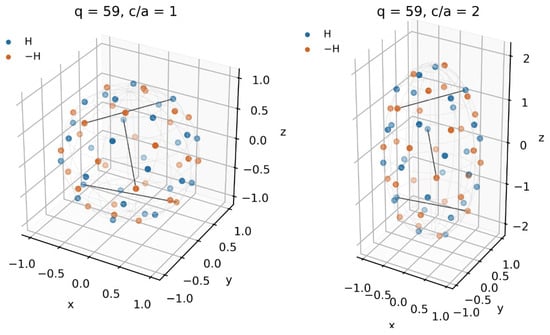
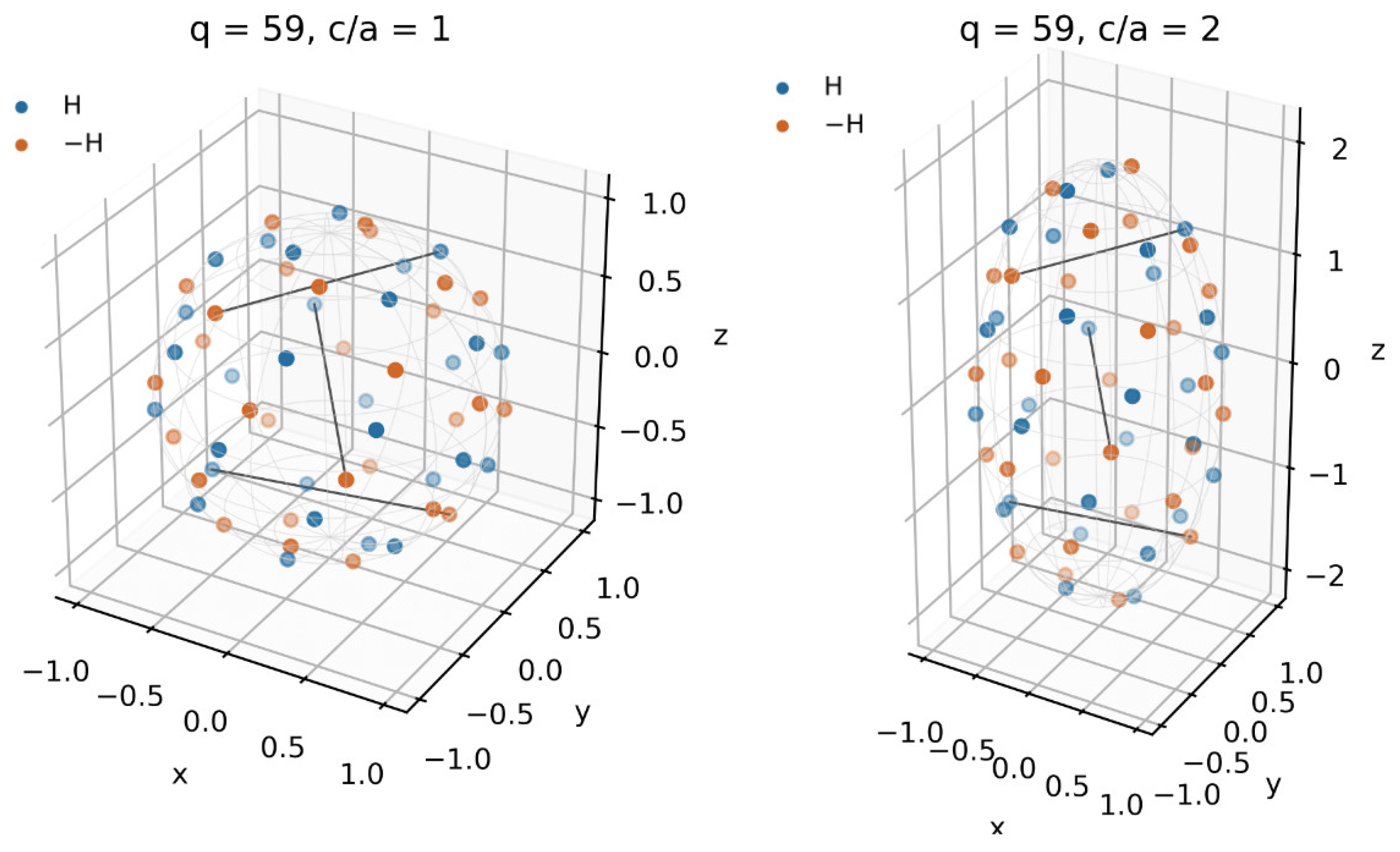
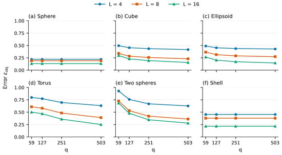
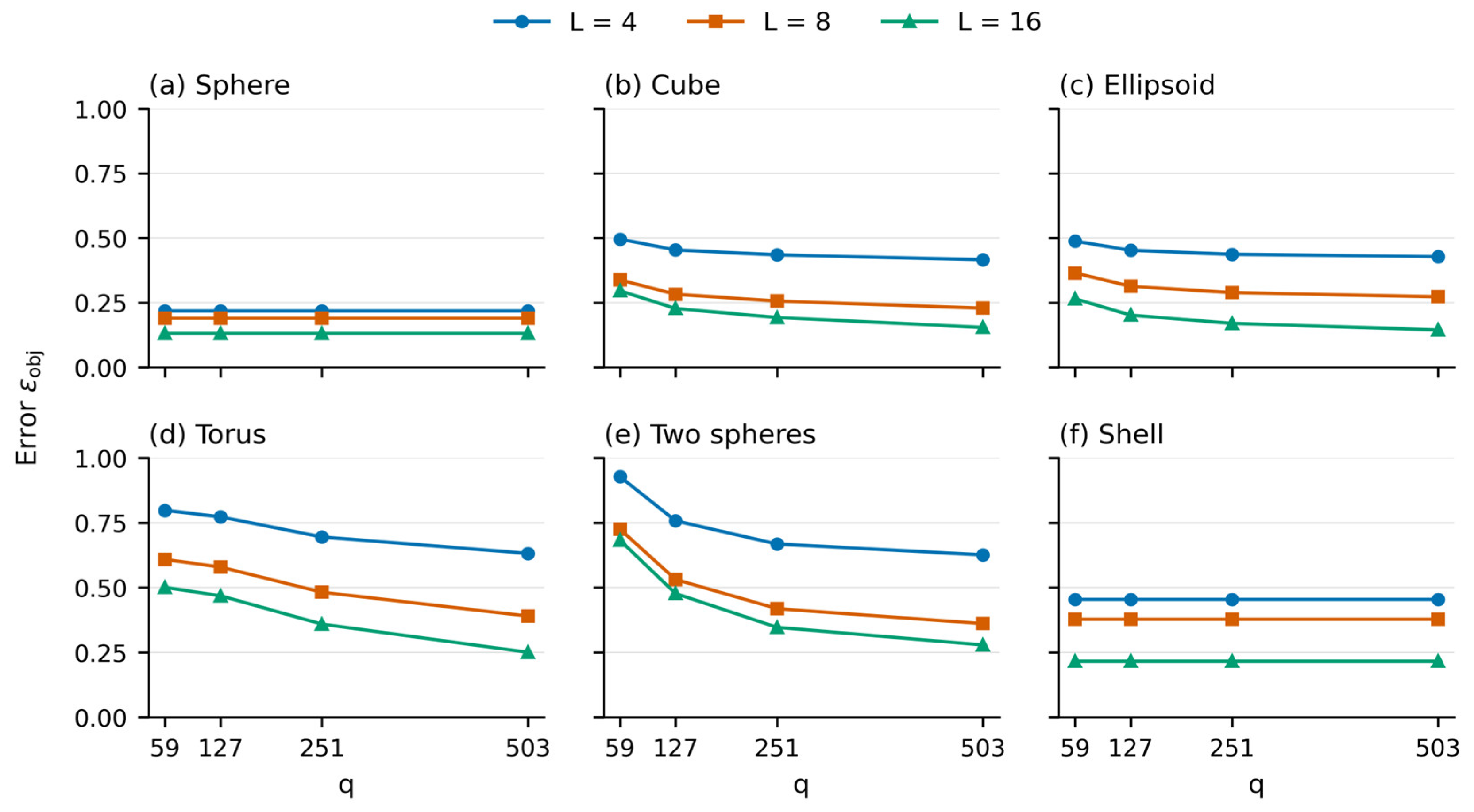
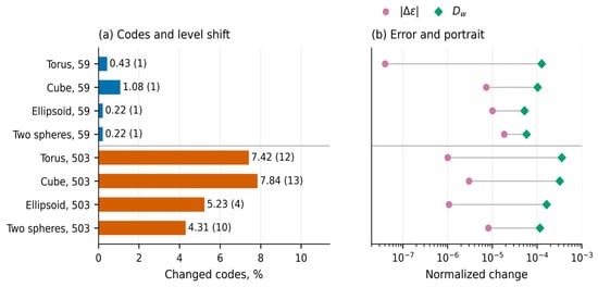
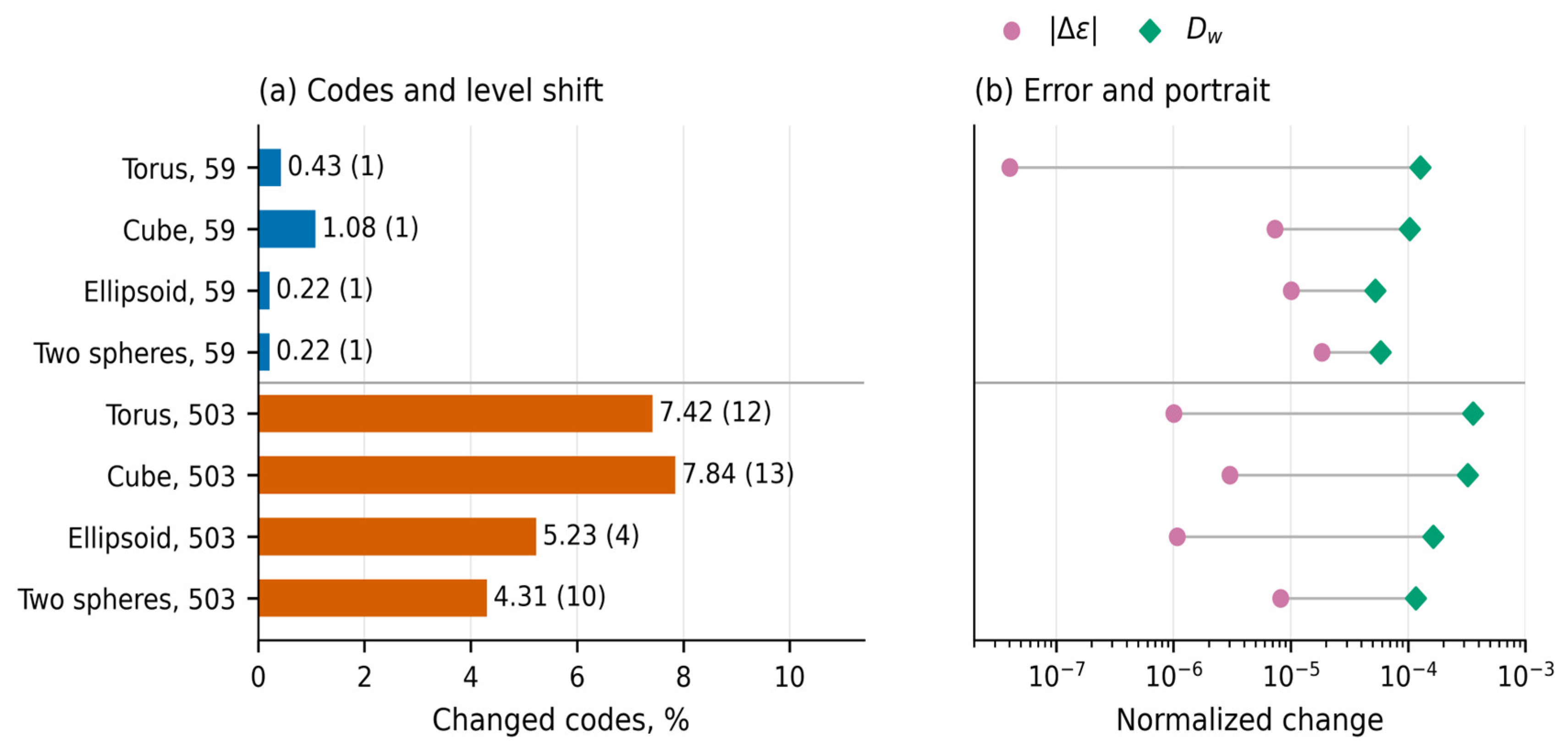
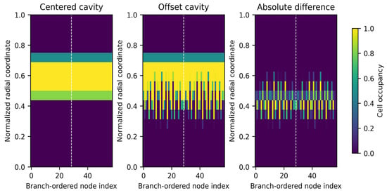
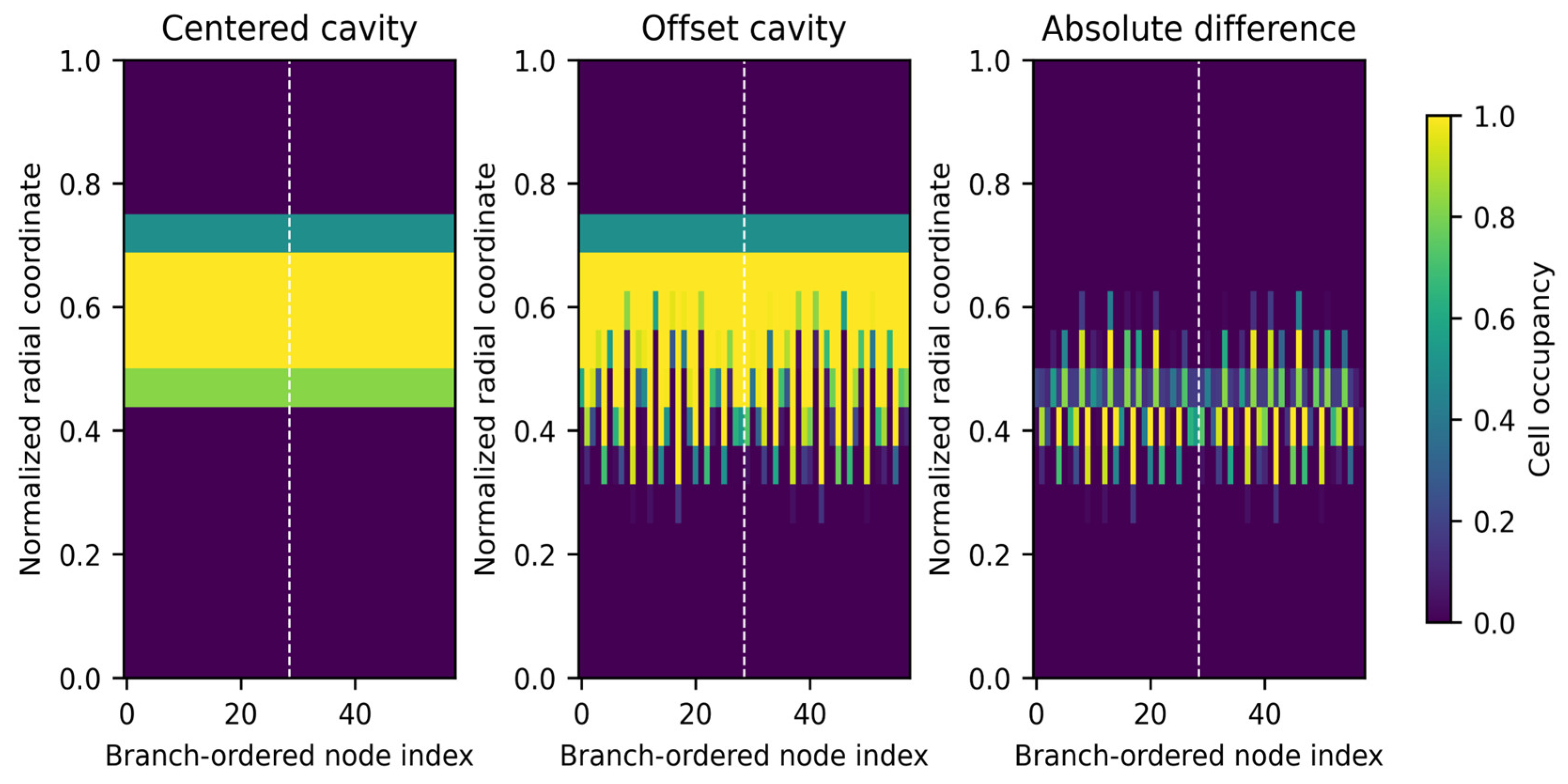
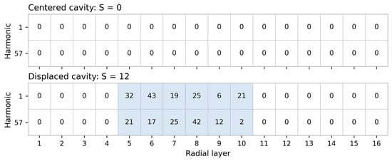
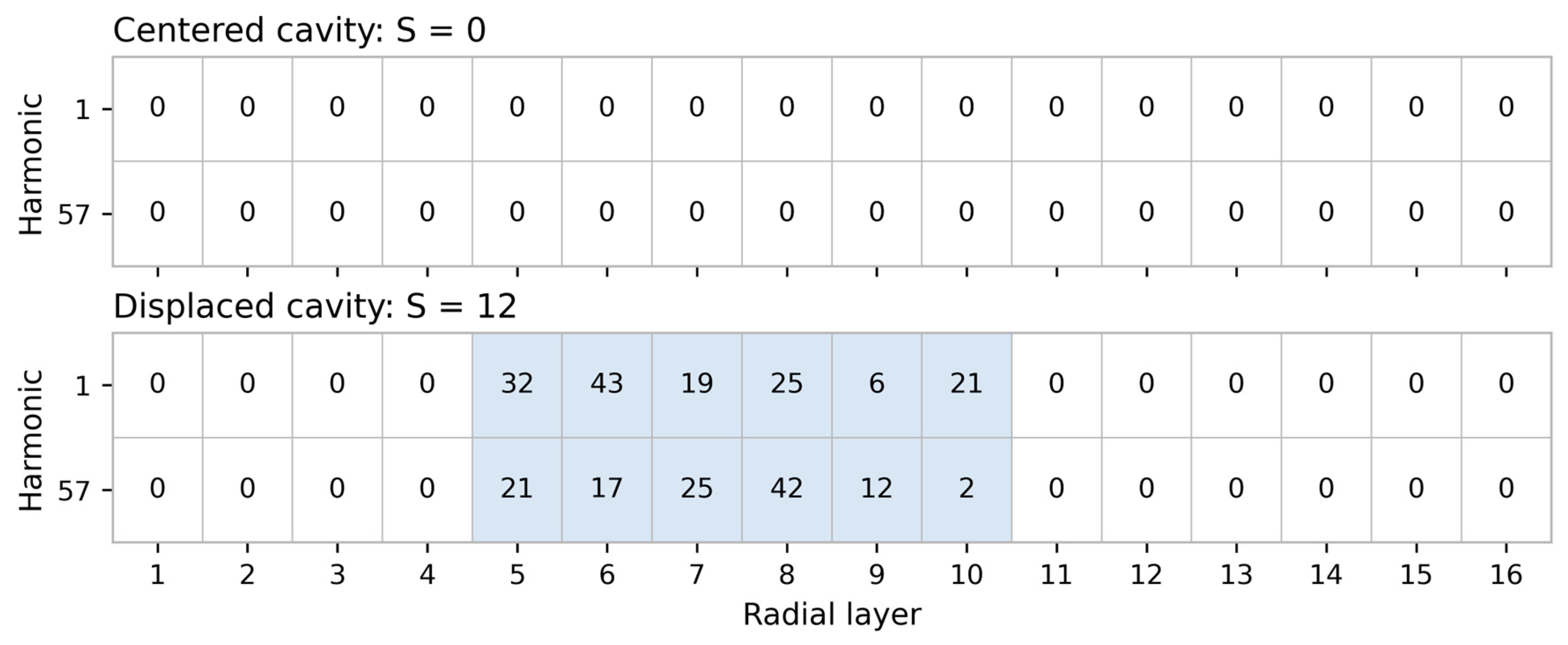
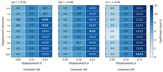
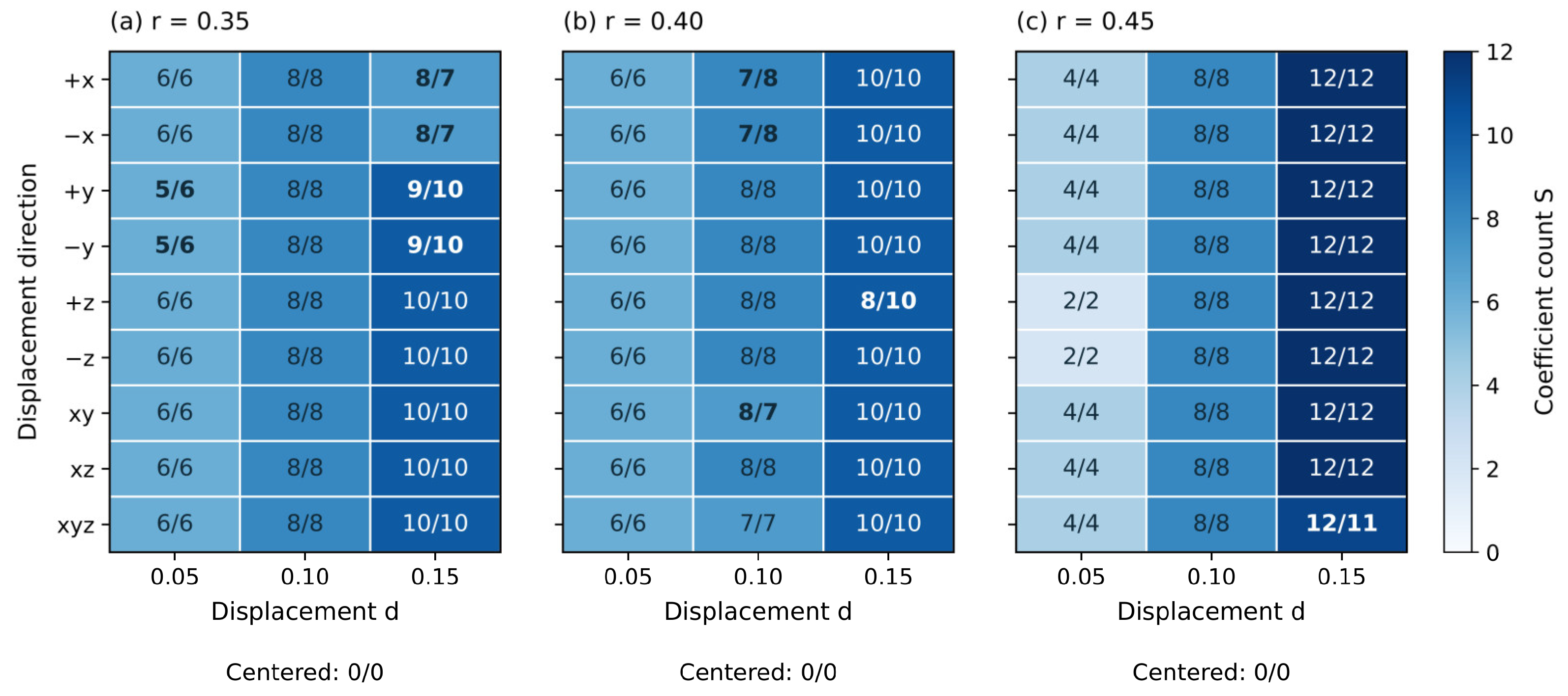

Disclaimer/Publisher’s Note: The statements, opinions and data contained in all publications are solely those of the individual author(s) and contributor(s) and not of MDPI and/or the editor(s). MDPI and/or the editor(s) disclaim responsibility for any injury to people or property resulting from any ideas, methods, instructions or products referred to in the content. |
© 2026 by the authors. Licensee MDPI, Basel, Switzerland. This article is an open access article distributed under the terms and conditions of the Creative Commons Attribution (CC BY) license.