


Abstract
The electrocardiogram (ECG) is a crucial non-invasive tool for diagnosing cardiovascular diseases. The standard 12-lead ECG configuration provides complementary spatio-temporal projections of cardiac electrical activity from distinct anatomical perspectives, enabling comprehensive pathological assessment. Unsupervised multi-lead ECG abnormality recognition has emerged as a promising approach, yet existing methods suffer from two limitations: insufficient attention to key pathological features and neglect of heterogeneous lead sensitivity. To address these issues, we propose the concept of lead-specific pathological sensitivity and develop the Lead-specific Pathological Sensitivity-aware Network (LPS-Net), comprising three modules: a Multi-scale Lead-specific Spatio-Temporal Encoder for discriminative representations, a Lead-specific Pathological Sensitivity-aware Topological Consensus Module that adaptively captures heterogeneous lead contributions, and an Asymmetric Hybrid Decoder that uses topological consensus to regularise reconstruction. Extensive experiments on four public 12-lead ECG benchmarks (PTB-XL, Chapman, CPSC-2018, and SPH) demonstrate the effectiveness of LPS-Net. On PTB-XL, LPS-Net achieves a clustering accuracy of 0.76 and a Macro F1 of 0.74 across five pathological superclass categories without any label information, outperforming the state-of-the-art method by 3%. Cross-dataset transfer experiments further confirm its generalisation ability. Ablation studies verify that the improvement originates specifically from the pathological-sensitivity formulation, and interpretability analyses reveal that the learned lead weight distributions align with clinical prior knowledge.
1. Introduction
The electrocardiogram (ECG) is a non-invasively acquired biomedical signal that depicts the electrical activity of the heart [1]. It records the spatio-temporal evolution of cardiac electrical activity during depolarisation and repolarisation, and electrophysiological abnormalities within the cardiac conduction system and myocardial cells are significantly reflected as morphological distortions in ECG waveforms [2]. This establishes the ECG as a gold standard biomarker for identifying abnormal heart conditions [3], which provides critical diagnostic utility in evaluating cardiac functional integrity and pathological evolution. Modern clinical practice predominantly utilises multi-lead systems to capture these activities from diverse spatial perspectives. However, the substantial increase in physiological data volume produced daily by cardiac monitors has intensified the requirement for automated analysis frameworks to assist in clinical interpretation [4,5].
The standard 12-lead ECG system, the most widely adopted multi-lead configuration in clinical cardiology, comprises three bipolar limb leads (I, II, III), three augmented limb leads (aVR, aVL, aVF), and six unipolar precordial leads (V1 through V6) [1,6]. These twelve leads collectively provide a comprehensive spatio-temporal projection of cardiac electrical activity from distinct anatomical vantage points. The six limb leads capture the frontal-plane projection of the cardiac electrical vector: leads I and aVL reflect left-lateral activity; leads II, III, and aVF reflect inferior activity; and lead aVR reflects right-superior activity. In contrast, the six precordial leads are positioned sequentially across the left chest wall and record the horizontal-plane projection, with V1 and V2 overlying the right ventricle and interventricular septum, V3 and V4 overlying the anterior wall of the left ventricle, and V5 and V6 overlying the lateral wall [7]. This multi-perspective design is clinically indispensable because cardiac pathologies are frequently spatially confined to specific myocardial regions, and their electrophysiological signatures may manifest prominently in only a subset of leads while remaining subtle or absent in others. Consequently, the 12-lead configuration provides complementary diagnostic information that no single lead can capture alone, underscoring both the clinical value of multi-lead acquisition and the analytical complexity inherent in processing heterogeneous multi-lead ECG data.
To satisfy the clinical requirement for efficient data analysis, numerous automated ECG auxiliary diagnosis methodologies have been proposed [8,9,10]. The majority of these approaches are grounded in supervised machine learning, which necessitates a substantial volume of cardiologist-supplied labels to provide essential prior knowledge. However, the acquisition of high-quality, expert-level annotations is exceptionally labour-intensive and costly, frequently resulting in existing datasets that are constrained in both scale and diversity. Such limitations hinder supervised models from encompassing the vast array of complex ECG patterns that emerge under various physiological and pathophysiological conditions. In this context, unsupervised multi-lead ECG analysis, specifically ECG abnormality recognition, has demonstrated significant potential. It aims to autonomously partition ECG samples into distinct groups by mining intrinsic structural characteristics and morphological similarities without the requirement for cardiologist-supplied labels. The technological landscape of ECG abnormality recognition has evolved from traditional machine learning algorithms, such as centroid-based and hierarchical clustering [11], toward advanced deep learning architectures, including deep autoencoders and generative models [12,13]. Compared to conventional methodologies, the primary advantage of these deep learning-based approaches lies in their capacity to automatically learn the most discriminative high-dimensional feature representations for abnormality recognition while bypassing tedious manual feature engineering. Despite these advancements, existing unsupervised ECG abnormality recognition paradigms still face two critical defects that hinder their clinical reliability:
- Representation with a lack of attention to key pathological features: Existing unsupervised ECG analysis lacks task-specific diagnostic guidance. It therefore relies on statistical representation compression schemes that project high-dimensional electrophysiological data into a low-dimensional latent space by reconstructing global signal fluctuations or minimising reconstruction errors. This non-task-oriented process biases models toward macro-statistical indicators such as intervals or heart rate, while neglecting subtle morphological features that hold diagnostic value [14]. For instance, vital pathological signatures like -segment deviations, P-wave morphology distortions, or T-wave inversions are fundamental to diagnosing myocardial ischemia, electrolyte imbalances, or atrial fibrillation. Yet these features are often discarded as insignificant numerical variance during unguided dimensionality reduction. Such neglect creates a structural mismatch between the learned mathematical representation space and the true clinical pathological manifold, ultimately harming the discriminative ability of recognition algorithms for complex electrophysiological signals.
- Neglect of Heterogeneous Lead Sensitivity: From an anatomical perspective, specific cardiac disorders, including localised myocardial infarction or chamber hypertrophy, typically exhibit distinct spatial constraints where abnormalities are confined to particular regions of the heart. Within a standard 12-lead ECG system, electrodes are distributed at various physical locations on the body surface to form multi-dimensional observational perspectives. Given the varying spatial relationship between each lead and the pathological site, their capacity to capture and characterise localised electrical evolutions differs significantly. As shown in Table 1, this phenomenon, defined as lead-specific pathological sensitivity, refers to the inherent heterogeneity in diagnostic utility across leads for a given pathological condition. A lead positioned at an optimal vantage point may demonstrate high discriminative power for a specific disease, while others distant from the pathology may only record non-specific reciprocal changes. Specifically, a localised pathology such as inferior myocardial infarction primarily manifests as -segment changes in leads , , and , whereas leads through may remain physiological. Existing unsupervised analysis frameworks typically concatenate features extracted from each lead or assign equal weights to all leads, which may introduce structural noise from non-sensitive leads and degrade the accuracy of the inferred pathological consensus.
Table 1.
Lead-specific pathological sensitivity across common cardiac conditions. Different ECG leads exhibit heterogeneous diagnostic utility depending on the spatial relationship between the electrode position and the affected myocardial region. Localised pathologies produce changes confined to specific lead groups, whereas diffuse processes affect multiple lead groups simultaneously [7,15].
To address these limitations, we propose a Lead-specific Pathological Sensitivity-aware Network (LPS-Net) for multi-lead ECG abnormality recognition. The proposed architecture comprises three synergistic components. First, the Multi-scale Lead-specific Spatio-Temporal Encoder (ML-SSTE) employs multi-scale dilated convolutions to model localised temporal evolutions and self-attention to capture global spatial correlations, thereby extracting discriminative latent manifolds and effectively mitigating redundancy across leads. Second, the Lead-specific Pathological Sensitivity-aware Topological Consensus Module (LPS-TCM) constructs multi-relationship graphs, including k-nearest-neighbour graphs and anchor graphs, for each lead, and then adaptively learns a weight tensor that captures the heterogeneous diagnostic contribution of different leads to various pathological clusters. Third, the Asymmetric Hybrid Decoder (AHD) takes the topological consensus inferred by LPS-TCM as a structural inductive bias to regularise the reconstruction process. Through Laplacian smoothing and high-resolution temporal projection, the decoder ensures that the learned features preserve morphological fidelity to the original signals while adhering to population-level pathological logic. By jointly optimising a reconstruction loss, a self-supervised classification loss, and the LPS-TCM objective, LPS-Net learns discriminative and clinically interpretable representations without requiring expert annotations.
The primary contributions of this work are summarised as follows:
- We propose the concept of lead-specific pathological sensitivity, which highlights that different ECG leads contribute unequally to the detection of spatially confined cardiac pathologies. To operationalise this concept, we propose a novel multi-lead ECG abnormality recognition model called LPS-Net. LPS-Net adaptively learns lead-specific characteristics, enhances the contribution of diagnostically informative leads to ECG signal abnormality recognition, and integrates the topological consensus representation across multiple leads.
- We propose an asymmetric autoencoder architecture for multi-lead ECG signals, which captures both local temporal and global spatial information through the Multi-scale Lead-specific Spatio-Temporal Encoder (ML-SSTE). During reconstruction, the decoder is guided by the lead-specific weight tensor learned by LPS-TCM, enabling the model to preserve pathologically relevant morphological features while suppressing noise from insensitive leads.
- We propose a joint optimisation strategy for training of the proposed framework. Extensive experiments on multiple public benchmarks show that LPS-Net consistently outperforms state-of-the-art methods in recognition accuracy and cross-dataset transferability.
2. Related Work
This section reviews the literature most pertinent to the proposed method, organised into four threads: (1) unsupervised ECG representation learning, spanning traditional clustering, deep clustering, and self-supervised approaches; (2) multi-lead ECG analysis, focusing on methods that exploit inter-lead relationships; (3) graph-based clustering, which provides the theoretical foundation for the proposed LPS-TCM module; and (4) interpretability in ECG analysis, which informs the design of the lead-specific sensitivity weight visualisation and validation strategy.
2.1. Unsupervised ECG Representation Learning
Unsupervised ECG analysis aims to partition signal samples into clinically meaningful groups without cardiologist-supplied labels, a paradigm commonly referred to as ECG abnormality recognition [3]. Early approaches employed traditional clustering algorithms on hand-crafted features. Lagerholm et al. [16] introduced self-organising maps combined with Hermite function descriptors to organise QRS complexes into morphological clusters. Balouchestani et al. [17] integrated compressed sensing theory with K-Means to accelerate clustering on large ECG datasets. He et al. [18] proposed wavelet tensor decomposition for 12-lead ECG, preserving spatial context through multi-way decomposition before applying Gaussian spectral clustering. While these methods demonstrated the feasibility of unsupervised ECG grouping, their reliance on manually engineered features limits their ability to capture complex morphological patterns associated with subtle pathologies.
The advent of deep clustering has enabled joint representation learning and cluster assignment within a unified framework. Xie et al. [19] introduced Deep Embedded Clustering (DEC), which jointly optimises a deep autoencoder and a KL-divergence-based clustering objective through soft assignment in a latent space. Subsequent developments, including Deep Adaptive Clustering (DAC) [20] and CatGAN [21], further improved clustering robustness through pairwise similarity learning and generative regularisation, respectively. Despite these advances, a limitation persists: these methods operate on a single representation space without exploiting the multi-lead spatial structure inherent to clinical ECG data, and their generic clustering objectives are decoupled from any domain-specific diagnostic guidance.
More recently, self-supervised learning (SSL) has been applied to ECG representation learning. Kiyasseh et al. [22] introduced contrastive learning across spatial, temporal, and patient dimensions, demonstrating that exploiting cardiac signal invariances outperforms generic methods such as the Simple Framework for Contrastive Learning of Visual Representations (SimCLR) and Bootstrap Your Own Latent (BYOL) in both linear evaluation and fine-tuning settings, and achieving strong generalisation with only 25% labelled training data. Mehari and Strodthoff [23] conducted a comprehensive benchmark of self-supervised methods, including Contrastive Predictive Coding (CPC), SimCLR, BYOL, and Swapping Assignments between Views (SWaV), on 12-lead ECG data, establishing standardised evaluation protocols on the PTB-XL dataset. Oh et al. [24] proposed lead-agnostic SSL that learns both local and global representations through random lead masking, enabling pre-training with arbitrary lead subsets. More recent efforts have explored domain-specific augmentations and multi-scale objectives [25,26,27] and Masked Autoencoder (MAE)-based pre-training for clinical early-warning applications [28,29]. In parallel, unsupervised representation learning has been used to reveal broad disease associations from ECG data: Friedman et al. [30] trained a denoising autoencoder on 12-lead ECGs and demonstrated that the learned latent space encodes associations with over 1200 diseases. Similarly, Yeung et al. [31] applied a variational autoencoder to UK Biobank ECGs, showing that latent factors capture clinically meaningful cardiac phenotypes and genetic associations. Gurniani et al. [32] employed a VAE combined with tree-based clustering to discover novel atrial fibrillation phenogroups stratified by disease risk, while Madrid et al. [33] demonstrated that unsupervised clustering of single-lead ECG features can identify heart failure risk clusters in coronary artery disease patients. While these studies demonstrate the clinical potential of unsupervised ECG analysis, they rely on generic feature extraction or post hoc clustering of learned embeddings, and the inter-lead pathological heterogeneity that motivates our work remains unaddressed.
2.2. Multi-Lead ECG Analysis
As discussed in the Introduction, most automated methods treat leads as independent channels or simply concatenate their features. Several studies have nevertheless recognised the importance of inter-lead relationships. Cheng et al. [34] proposed the Lead Feature Guide Network (LFG-Net), which uses SHAP-based analysis to identify high-contribution leads and guides the classification model to focus on them, recognising that different leads contribute unequally to diagnosis. In a related direction, Zhang et al. [35] treated multi-lead ECG as a 2D matrix and employed multi-scale 2D convolutions with squeeze-and-excitation modules to capture cross-lead dependencies. More recently, Graph Neural Networks have been applied to model inter-lead topological relationships: Chen et al. [36] constructed feature graphs and topology graphs with leads as nodes, adaptively fusing information through graph convolution and attention mechanisms for arrhythmia classification.
However, a notable limitation of this body of work is that all existing methods that explicitly model lead-specific contributions operate in a supervised setting, requiring labelled data for training. In the unsupervised scenario, where labels are unavailable, no existing method adaptively weights leads according to their pathological relevance. This leaves a significant gap: the heterogeneous diagnostic sensitivity across leads, established in clinical cardiology, remains unexploited by unsupervised ECG analysis frameworks.
2.3. Graph-Based Clustering and Topological Optimisation
Graph-based clustering provides the theoretical foundation for the proposed LPS-TCM module. Spectral clustering methods partition data by optimising graph-cut objectives on similarity graphs, offering advantages over centroid-based approaches for non-convex cluster structures. Nie et al. [37] proposed clustering with adaptive neighbours, where the graph affinity matrix and cluster assignment are jointly optimised through an iterative scheme. This framework was later extended by a coordinate descent method [38] that efficiently solves the K-Means objective with convergence guarantees. These optimisation strategies inspire the alternating optimisation design of LPS-TCM, where the lead-specific sensitivity weights and the clustering indicator matrix are iteratively refined.
In the biomedical signal domain, graph-based methods have been primarily applied in supervised settings, for instance, constructing spatial graphs over ECG leads for arrhythmia classification [36]. The application of graph-cut optimisation to unsupervised multi-lead ECG abnormality recognition, particularly with adaptive lead weighting, remains unexplored. The proposed LPS-TCM module fills this void by constructing multi-relation graphs (k-nearest-neighbour (kNN) graphs and anchor graphs) over per-lead latent representations and optimising a mixed-cut objective that is jointly modulated by learnable lead-specific sensitivity weights.
2.4. Interpretability in ECG Analysis
Clinical interpretability is a critical requirement for deploying automated ECG analysis systems in practice. In the supervised setting, Cheng et al. [34] employed SHAP-based analysis to identify high-contribution leads for ECG classification, providing post hoc explanations of model decisions. Attention mechanisms have also been widely adopted to highlight diagnostically relevant signal regions: Zhang et al. [35] used squeeze-and-excitation modules to recalibrate channel-wise feature importance, while Chen et al. [36] employed graph attention to identify influential inter-lead relationships. More recently, Yeung et al. [31] demonstrated that latent factors learned by a variational autoencoder correlate with conventional ECG parameters, enabling clinically interpretable representation learning without explicit supervision.
Nevertheless, interpretability in the unsupervised setting remains largely unexplored. Existing deep clustering methods provide cluster assignments without explanatory mechanisms, making it difficult for clinicians to assess the validity of discovered patterns. To this end, LPS-Net incorporates an explicit lead-specific weight tensor that quantifies the diagnostic contribution of each lead to each pathological cluster, thereby enabling direct clinical validation through weight distribution visualisation, statistical significance testing, and lead-specific noise perturbation experiments.
Overall, the proposed LPS-Net bridges these gaps through an integrated encoder, LPS-TCM, and decoder architecture, where lead-specific sensitivity weights learned by the clustering module feed back into both representation learning and signal reconstruction.
3. Methodology
3.1. Problem Formulation
The objective of this study is to perform multi-lead abnormality recognition on ECG physiological signals to identify distinct pathological patterns without prior labelling. Given a dataset consisting of m lead views, each signal matrix contains the physiological recordings of n samples over T time steps for the v-th lead. The task is to identify k distinct pathological patterns among the n samples by leveraging the complementary information across all m leads.
3.2. General Framework Overview
As illustrated in Figure 1, LPS-Net consists of three cascaded modules that operate in a unified end-to-end framework. The data flow proceeds as follows. The input consists of preprocessed 12-lead ECG signals , where each lead’s signal is processed independently by the Multi-scale Lead-specific Spatio-Temporal Encoder (ML-SSTE). Within the ML-SSTE block, each lead signal passes through L stacked dilated convolutional layers with exponentially increasing dilation rates, followed by squeeze-and-excitation (SE) channel recalibration, Batch Normalisation (BN), and residual connections. A temporal self-attention pooling layer then aggregates the serialised features into a compact lead-level embedding for each lead v. The per-lead embeddings are then routed to two parallel branches. In the first branch, the Multi-lead Consensus Classification Network concatenates all lead embeddings into a fused representation and projects it through a Multi-Layer Perceptron (MLP) with Softmax activation to produce the final cluster assignment probabilities . In the second branch, the Lead-specific Pathological Sensitivity-aware Topological Consensus Module (LPS-TCM) constructs two types of graphs, namely k-nearest-neighbour (kNN) graphs and anchor graphs , for each lead, and learns a lead-specific weight tensor that captures the heterogeneous diagnostic contribution of different leads to various pathological clusters. The LPS-TCM outputs a consensus indicator matrix that serves as pseudo-labels for training the classification network via the self-supervised classification loss . The Asymmetric Hybrid Decoder (AHD) takes the per-lead embeddings and the topological consensus as input. It constructs lead-specific weighted topological operators that combine the kNN and anchor graphs modulated by cluster-specific masks and lead-specific weights. These operators perform Laplacian smoothing via a Graph Neural Network (GNN) to recalibrate the embeddings toward manifold alignment, followed by a Temporal Projection Operator (TPO) that maps the recalibrated features back to the original signal space, producing reconstructed signals . The entire framework is trained via an alternating optimisation strategy with two sub-problems executed iteratively: (i) parameter optimisation, which updates the encoder, classification network, and decoder using the AdamW optimiser with a One-Cycle learning rate schedule, guided by a joint loss combining reconstruction loss and self-supervised classification loss , and (ii) Topological Consensus Inference, which updates and using a coordinate descent method while keeping the network parameters fixed. This alternating process ensures that the neural network’s latent space remains structurally aligned with the population-level topological consensus.
Figure 1.
Overall framework of the proposed LPS-Net. The architecture comprises three core modules: (1) Multi-scale Lead-specific Spatio-Temporal Encoder (ML-SSTE) producing per-lead latent representations ; (2) Lead-specific Pathological Sensitivity-aware Topological Consensus Module (LPS-TCM) inferring a consensus indicator matrix and lead-specific weight tensor via kNN and anchor graphs; and (3) Asymmetric Hybrid Decoder (AHD) reconstructing signals under topological guidance. Additionally, a Multi-lead Consensus Classification Network produces the final cluster assignment probabilities . The framework is trained via alternating optimisation: consensus inference (frozen network) and parameter optimisation (AdamW, joint reconstruction and classification losses). Red arrows indicate data flow; blue arrows indicate loss feedback. Dashed boxes delineate major functional modules, and dashed circles highlight the multi-scale branches.
3.3. Multi-Scale Lead-Specific Spatio-Temporal Encoder
The Multi-Scale Lead-Specific Spatio-Temporal Encoder (ML-SSTE) is designed to characterise the intricate spatio-temporal dependencies within multi-lead ECG data by concurrently encoding localised temporal morphological evolutions and global spatial projection correlations across multiple resolution scales. Specifically, the module processes the preprocessed signal matrices as input and employs multi-scale dilated convolutions to capture temporal dependencies across different receptive fields.
The encoder performs multi-scale modelling by stacking L layers of discrete dilated convolutions. To this end, each layer is configured with an exponentially increasing dilation rate , allowing the effective receptive field to expand progressively with network depth without compromising temporal resolution:
where denotes the intermediate feature mapping, and represents the lead-specific learnable kernels of temporal size K. Specifically, for the initial layer (), the input is defined as the signal sequence .
Upon obtaining the initial temporal mappings, a squeeze-and-excitation (SE) unit is integrated for channel-wise recalibration. This unit first aggregates temporal information to generate a channel-wise descriptor and subsequently derives a channel-wise importance weight vector by learning non-linear dependencies between channels. These weights are utilised to recalibrate the features , resulting in the recalibrated feature vector :
Furthermore, incorporating Batch Normalisation (BN) and residual connections, the final output of layer l is defined as
where is the ReLU activation function. After L layers of evolution, the serialised latent manifold for the v-th lead is denoted as .
Finally, to transform the serialised local features into lead-level global descriptors, the encoder introduces a self-attention mechanism. This mechanism identifies significant temporal segments by computing the attention scores through the following scoring function:
where and are learnable parameters. The scoring values are normalised via a Softmax function to obtain the temporal weight coefficients :
The final encoding matrix for lead v is then calculated as the weighted aggregation of the sequence features:
3.4. Multi-Lead Consensus Classification Network
This module establishes a mapping from the high-dimensional latent space to the clinical diagnostic domain to derive consensus classification results. The network takes the multi-lead latent representations generated by ML-SSTE as input. To integrate multi-lead information, are concatenated and projected into a unified discriminative space of dimension , yielding the global fused feature matrix :
where and are trainable parameters. This fusion enhances overall discriminability by facilitating cross-lead semantic completion. Subsequently, the matrix is processed by a standard Multi-Layer Perceptron (MLP) architecture equipped with Batch Normalisation and Dropout. Finally, a Softmax activation function maps the output into a predicted probability distribution across k potential pathological clusters:
where denotes the set of parameters within the classification network.
3.5. Lead-Specific Pathological Sensitivity-Aware Topological Consensus Module
The Lead-specific Pathological Sensitivity-aware Topological Consensus Module (LPS-TCM) aims to extract discriminative pathological patterns by mining the topological consensus across multiple leads. Recognising that different ECG leads exhibit varying diagnostic contributions to specific diseases, this module explicitly incorporates lead-specific pathological sensitivity as a structural inductive bias to guide the representation alignment process.
For multi-lead latent representations , our method constructs m -nearest-neighbour (kNN) graphs denoted as and m anchor graphs denoted as , where denotes the number of nearest neighbours (distinct from k, the number of clusters, used in subsequent sections). Specifically, the kNN graph of v-th lead is constructed via solving the following optimisation problem to search adaptive neighbours for samples under v-th lead:
To avoid trivial solutions where the nearest sample becomes the sole neighbour of with probability 1 while all other samples are excluded, a regularisation term is introduced to problem (9):
where is the trade-off parameter.
Inspired by [38], a sparse , whose each row has nonzero values, can be learned via denoting setting ; thus, the optimal solution of is
In addition, for constructing the anchor graph of the v-th lead, we utilise the k-means algorithm to search k centres as anchors. Via denoting the indicator matrix as the clustering result of the k-means algorithm, the sample–anchor bipartite graph is subsequently constructed as follows:
Correspondingly, we obtain the anchor graph from via the following transformation:
where is defined as .
From the multi-lead and multi-relationship graphs and , LPS-TCM learns a unified indicator matrix as pseudo-labels for guiding the classification network via a mixed cut model, which is defined as the following optimisation problem:
where denotes the set of indicator matrices whose rows are one-hot vectors; i.e., each row of has exactly one entry equal to 1 and the rest equal to 0, and is the degree matrix of .
More importantly, LPS-TCM learns a lead-specific pathological sensitivity weight coefficient tensor to mine local patterns, weights the constructed multi-lead and multi-relation graph, and guides the model to integrate fine-grained information, resulting in a more robust consensus recognition result. The total objective function can be given as follows:
where we denote for convenience. is the normalisation constraint for variable .
3.6. Asymmetric Hybrid Decoder Guided by Lead-Specific Pathological Sensitivity
An Asymmetric Hybrid Decoder (AHD) is designed to execute the inverse mapping for embedding from high-dimensional latent manifolds back to the original physiological signal space. The structural hallmark of this architecture is a multi-channel hybrid decoding head, which explicitly incorporates the lead-specific pathological sensitivity identified by the LPS-TCM as a structural inductive bias to regularise the reconstruction process. Lead-specific pathological sensitivity accounts for the heterogeneous sensitivity of physiological leads to specific pathological patterns, manifesting as non-uniform structural effectiveness across different leads. To capture these fine-grained structural nuances, the decoder synergistically utilises the consensus indicator matrix and the lead-specific pathological sensitivity weight tensor derived from the LPS-TCM to customise exclusive topological channels for each lead.
The adaptive synthesis of multi-channel topological manifolds serves as the cornerstone for high-fidelity reconstruction. For each lead , the decoder integrates the adaptive k-nearest neighbour graph , which characterises localised manifold structures, with the anchor graph that captures global distribution properties. By introducing cluster-specific masks , defined by the indicator matrix , the model precisely identifies the topological boundaries of pathologically homogeneous samples within the sample space. The unified, lead-specific weighted topological operator is constructed as follows:
where the weight coefficients empower the model to dynamically calibrate the contributions of different relationship graphs. This mechanism ensures that the feature aggregation process remains focused on highly discriminative local pathological manifolds, effectively filtering out stochastic noise through population-level collaboration.
Lead-specific parallel representation recalibration subsequently unfolds within the non-Euclidean space. The decoder utilises a symmetric normalised Laplacian smoothing operator, , to guide the encoded features toward manifold alignment consistent with the inferred topological consensus by a Graph Neural Network with F layers, where is the degree matrix of . The evolution operation for the l-th layer in each lead view follows
where is the embedding of the v-th lead samples in layer l, , and denotes the lead-shared trainable weight tensor at layer l. Through this inter-sample message-passing mechanism, the decoder assimilates structural consensus from the topological neighbourhood, enhancing feature discriminability in channels with high pathological sensitivity and facilitating the convergence of feature distributions toward their respective pathological centres.
The inverse mapping and reshaping of temporal morphology constitute the final stage of the decoding process, responsible for translating the recalibrated abstract semantics back into physical signals. To mitigate the inherent over-smoothing tendency of graph convolutional operators, a high-resolution temporal projection operator (TPO) is embedded at the output end of the decoder. This operator bridges the dimensional gap by mapping latent variables back to the original temporal space , aiming to precisely reconstruct microscopic waveform details, such as QRS complexes:
where and represent the learnable weights and bias of the reconstruction layers, respectively. This serialised topological recalibration then temporal reshaping paradigm ensures that the reconstructed signal maintains high physiological fidelity while adhering to the inferred pathological logic.
3.7. Joint Optimisation Strategy
To empower the model with the capability to extract discriminative latent features and learn the pathological discrimination logic guided by lead-specific pathological sensitivity, this study constructs an efficient joint optimisation strategy. Given that the total objective function is non-convex with respect to both network parameters and topological variables (), an alternating iterative optimisation method is adopted to reach a stable solution. Specifically, the global optimisation task is decomposed into two alternating sub-problems: Topological Consensus Inference and Parameter Optimisation via Multi-task Learning. By iteratively solving one sub-problem while fixing the variables of the other, the model ensures that the neural network’s latent space remains structurally aligned with the population-level topological consensus inferred from the multi-relationship graphs.
3.7.1. Components of Loss Functions
The proposed optimisation strategy aims to strengthen the model’s representational efficacy and diagnostic effectiveness by minimising a joint loss function , which integrates topological, morphological, and semantic constraints:
where represents the clustering objective function capturing lead-specific pathological sensitivity as problem (15) illustrates, while and are hyperparameters balancing the weights of individual sub-tasks. By combining self-supervised and pseudo-supervised objectives, the model minimises the following specialised losses:
- Reconstruction loss (): This term utilises explicit reconstruction constraints to compel the encoder to extract essential morphological features from original signals. It is defined as the sum of Frobenius norms between the original signals and the reconstructed signals across all m leads:
- Self-supervised classification loss (): This term injects population-level topological structures into the neural network by treating the inferred cluster assignments as supervision signals. Using a cross-entropy function, it minimises the discrepancy between the classifier’s predicted distribution and the topological pseudo-labels :
3.7.2. Topological Consensus Inference
In this sub-problem, the network parameters and the resulting latent representations are fixed, simplifying the optimisation to . The core of this stage is to infer the lead-specific pathological sensitivity weight tensor and the consensus indicator matrix to capture the lead-disease bias inherent in the data.
We propose following iterative methods to solve optimisation involved in LPS-TCM.
- Optimise
We first give sub-problem w.r.t. as Problem (22):
According to the Cauchy–Schwarz inequality,
In general, with holding the optimality conditions, problem (15) can be solved via solving a more concise form as problem (24):
- Optimise
can be optimised by solving problem (24) via a coordinate descent method, as rows of are independent in optimisation. To be specific, suppose is the current solution; when the j-th row of is optimised by fixing the other rows, the optimal solution (denoted as ) can be determined by choosing a proper one among the k candidates defined as , where is a one-hot row vector with the s-th entry equal to 1. For better illustration, we introduce auxiliary indicator matrices whose j-th row is the corresponding while the remaining rows are the same as . Based on the above discussion, the optima can be given as follows:
Since the difference between and only exists in the j-th row, denoting as a k-dimensional zero vector, we transform the optimisation problem in Equation (25) into the following problem to reduce redundant calculations:
Furthermore, suppose , and have been precalculated; problem (26) can be solved more succinctly. Considering two cases related to the s, suppose d indicates that ; we reduce the computation costs of problem (26) via the following transformations based on known information:
Let denote a one-hot column vector with the j-th entry equal to 1. We consider two cases:
- (1)
- If , we have and ; then,
- (2)
- If , we have and ; then,
Since has been solved, i.e., is the optima of problem (26), we need to update the precalculation for the subsequent iteration if . The following two cases should be considered. The updating of precalculation just needs some calculations conducted in the previous process, which further makes the optimisation more efficient.
3.7.3. Parameter Optimisation via Multi-Task Learning
With the indicator matrix and fixed, this sub-problem focuses on updating the neural network parameters , including the encoder, decoder, and classification head. The objective is optimised using the AdamW optimiser [39] with a One-Cycle learning rate schedule [40]:
where denotes the learning rate at step t governed by the One-Cycle policy, which anneals the rate from an initial warm-up to a peak value and then decays to a minimum. In this stage, the reconstruction loss ensures the extraction of essential morphological features, while enforces the latent representations to adhere to the manifold constraints established by the inferred topological consensus. This alternating process enables end-to-end learning that bridges low-level signal fidelity with high-level pathological logic.
3.7.4. Algorithm Summary and Training/Testing Protocol
To clarify the complete training and inference pipeline, we summarise the LPS-Net algorithm below. The training phase consists of unsupervised pre-training via alternating optimisation (Algorithm 1), which requires no label information. The testing phase encompasses three evaluation scenarios: (1) Direct clustering evaluation, where the pre-trained model is applied to the test set and the Multi-lead Consensus Classification Network produces cluster assignments (via arg max) that are compared to ground-truth labels via Hungarian mapping. (2) Cross-dataset clustering transfer, where the encoder is pre-trained on a source dataset and frozen; on the target dataset, a new classification network and LPS-TCM are trained from scratch in a fully unsupervised manner (no target labels), using the frozen encoder’s representations as input. (3) Interpretability analysis, where the pre-trained model clusters MI subtype samples and the learned lead-specific weights are visualised. In all testing scenarios, no labels are used during inference; labels are only used for post hoc evaluation via clustering metrics.
| Algorithm 1: LPS-Net Training (Unsupervised Pre-training). |
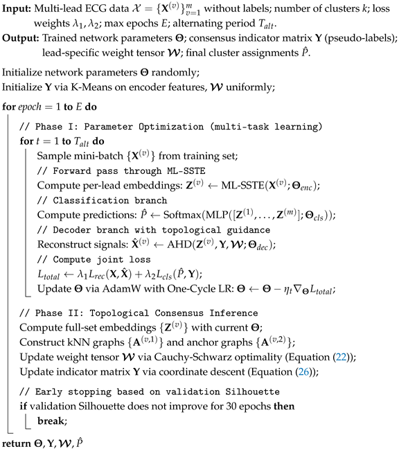 |
Testing Protocol. During inference, the trained encoder and Multi-lead Consensus Classification Network are applied to the test set. The encoder extracts test-set embeddings , and the classification network produces predicted cluster probabilities . The final cluster assignment for each sample is obtained via arg maxc . Note that LPS-TCM is not invoked during inference; its role is confined to the training phase, where it provides pseudo-labels and weight tensor to guide representation learning. The resulting assignments are evaluated against ground-truth labels using Clustering Accuracy, Macro , ARI, NMI, Purity, and Silhouette. For cross-dataset transfer, only the encoder pre-trained on a source dataset is frozen; on the target dataset, a new classification network and LPS-TCM are trained from scratch in a fully unsupervised manner using the frozen encoder’s representations, with the number of clusters k set according to the clinical taxonomy of the target dataset (e.g., for PTB-XL superclasses). No target-domain labels are used at any stage.
4. Experiments
To comprehensively evaluate the proposed LPS-Net, we conduct experiments on four public ECG benchmarks. The evaluation protocol comprises four parts. First, direct clustering evaluation is performed to assess the unsupervised abnormality recognition capability of LPS-Net, using standard clustering metrics (Silhouette, ARI, NMI, Purity, Clustering Accuracy, and Macro ) against representative unsupervised clustering baselines. Second, cross-dataset clustering transferability is evaluated to test generalisation: the encoder is pre-trained on a source dataset and frozen, after which the clustering head is re-trained in an unsupervised manner on a target dataset without any target-domain labels. Third, ablation studies quantify the contribution of each core component. Fourth, interpretability analysis verifies the clinical consistency of the learned lead weights. All models are trained under identical preprocessing and hardware settings to ensure fair comparison.
4.1. Datasets
The performance of the proposed framework is validated on four representative large-scale publicly available 12-lead electrocardiogram (ECG) benchmark datasets:
- PTB-XL [41]: This dataset comprises 21,837 recordings of 10 s length from 18,885 patients, with an original sampling frequency of 500 Hz. As one of the most widely adopted benchmarks in clinical ECG analysis, its diagnostic labels follow the SCP-ECG (Standard Communications Protocol for Computer-Assisted Electrocardiography) standard and are categorised into five primary superclasses: Normal ECG (NORM), Myocardial Infarction (MI), ST/T Change (STTC), Conduction Disturbance (CD), and Hypertrophy (HYP).
- Chapman–Shaoxing [42]: This collection features 12-lead recordings from 10,656 subjects, with all signals being 10 s long and sampled at 500 Hz. The dataset focuses on distinguishing fundamental cardiac rhythms and is condensed into four clinically significant superclasses: Atrial Fibrillation (AFIB), General Supraventricular Tachycardia (GSVT), Sinus Bradycardia (SB), and Sinus Rhythm (SR).
- CPSC-2018 [43]: Derived from the 1st China Physiological Signal Challenge, this multi-centre dataset includes 6877 12-lead recordings provided by 11 hospitals, sampled at 500 Hz with durations ranging from 6 to 60 s. It encompasses nine common pathological categories and rhythms: Normal, Atrial Fibrillation (AF), First-degree Atrioventricular Block (I-AVB), Left Bundle Branch Block (LBBB), Right Bundle Branch Block (RBBB), Premature Atrial Contraction (PAC), Premature Ventricular Contraction (PVC), ST-segment Depression (STD), and ST-segment Elevation (STE).
- SPH [44]: Provided by Shandong Provincial Hospital, this dataset contains 25,770 12-lead ECG recordings sampled at 500 Hz. A distinctive feature of SPH is its extremely granular labelling system, covering as many as 68 diagnostic categories. This study utilises it as a stress-test benchmark to evaluate the generalisation capability of the representations under extreme long-tail distributions and complex pathological combinations.
4.2. Baselines
To evaluate the efficacy of the proposed framework, we compare our model against a diverse set of unsupervised clustering baselines spanning different methodological trajectories:
- K-Means (raw): K-Means clustering directly applied to raw ECG signals, serving as a lower bound.
- CVAE + K-Means: A convolutional variational autoencoder for unsupervised feature extraction, followed by K-Means clustering, representing the generative route.
- DEC [19]: Deep Embedded Clustering, jointly optimising a deep autoencoder and a KL-divergence-based clustering objective.
- DFA + WE + K-Means: Detrended fluctuation analysis (DFA) and wavelet entropy (WE) features fed into K-Means, representing the traditional feature-engineering route.
- IDEC [45]: Improved DEC that jointly fine-tunes the encoder and clustering head to prevent feature drift.
- MDFC-AC [46]: Multimodal Deep Fusion Clustering with Anti-Collapse attention, representing the current state of the art for unsupervised 12-lead ECG clustering on PTB-XL.
- SMC [47]: Sequential MAE-Clustering, originally proposed for single-lead heartbeat classification on MIT-BIH using Gramian Angular Field (GAF) image conversion and linear probing evaluation. We adapt it to our unsupervised multi-lead ECG clustering setting by applying the Sequential MAE (SM) network and GMM with ProtoNCE loss directly to multi-lead ECG features, representing the self-supervised MAE route.
For the cross-dataset clustering transferability experiment, we select DEC and MDFC-AC as comparison methods, as they represent the strongest deep clustering baselines capable of unsupervised pre-training and cross-domain clustering.
4.3. Evaluation Metrics
To quantitatively evaluate the unsupervised abnormality recognition capability of the learned representations, we adopt six standard clustering metrics: (1) Silhouette Score (Sil) [48], measuring intra-cluster cohesion versus inter-cluster separation; (2) Adjusted Rand Index (ARI) [49], quantifying agreement between clustering assignments and ground-truth labels adjusted for chance; (3) Normalised Mutual Information (NMI) [50], measuring the mutual information between cluster assignments and true labels normalised by entropy; (4) Clustering Purity, computing the fraction of samples belonging to the majority class in each cluster; (5) Clustering Accuracy (Acc), obtained by optimally mapping cluster assignments to ground-truth labels via the Hungarian algorithm [51]; and (6) Macro -score computed after the same Hungarian mapping. All metrics range from 0 to 1, with higher values indicating better clustering quality. For cross-dataset transferability, we report Acc and NMI as representative metrics.
4.4. Implementation Details
All signals are resampled to 100 Hz for the main experiments. For the clustering evaluation, experiments are additionally conducted at the original 500 Hz sampling rate to enable direct comparison with MDFC-AC. A zero-phase bandpass filter with a frequency range of 0.5–40 Hz is applied. Input samples are 2.5 s segments (250 points at 100 Hz, 1250 points at 500 Hz) extracted via random sliding windows with Z-score normalisation.
Data Splitting. For each dataset, we adopt a patient-level train/validation/test split to prevent recordings or segments from the same patient from appearing in different subsets, thereby avoiding data leakage. Specifically, for PTB-XL, we follow the official split (folds 0–7 for training, fold 8 for validation, fold 9 for testing), which is inherently patient-stratified. For Chapman–Shaoxing, CPSC-2018, and SPH, we partition the patient list into 80%/10%/10% for train/validation/test, respectively, ensuring that all recordings from a given patient are assigned to the same subset. During training, 2.5 s segments are randomly extracted from each recording with augmentation; during evaluation, each recording is segmented into non-overlapping 2.5 s windows, and the final prediction is obtained by averaging the segment-level outputs.
Hyperparameter Selection. The ML-SSTE encoder utilises an embedding dimension of 128. The loss balancing coefficients and are both selected from , and the regularisation parameter is selected from . Hyperparameters are chosen by grid search on the validation set, optimising Silhouette score for clustering evaluation. The number of nearest neighbours for the k-NN graph in LPS-TCM is set to , and the number of anchors for the anchor graph equals the number of clusters. The AdamW optimiser [39] is used with a One-Cycle learning rate schedule [40]. The peak learning rate is within the range of to . Pre-training is conducted for 300 epochs with a batch size of 128. The alternating period , which determines the number of parameter optimisation steps between consecutive topological consensus updates, is set to 5. Early stopping with a patience of 30 epochs is applied based on validation performance.
Determination of Cluster Number. For clustering evaluation on PTB-XL, the number of clusters is set to , matching the five superclass labels (NORM, MI, STTC, CD, HYP). For the ablation study and interpretability analysis on MI subtypes, k is set to 4, corresponding to the four MI subtypes (Anterior, Inferior, Lateral, Extensive). In all cases, k is determined by the clinical taxonomy of the target dataset and is not learned from data, ensuring that the evaluation reflects the alignment between discovered clusters and clinically defined categories.
All experiments are implemented using PyTorch 2.10.0 on an NVIDIA RTX 4090 GPU workstation. To ensure statistical robustness, all reported results are averaged over five independent runs with different random seeds. We report mean ± standard deviation for all experiments.
4.5. Clustering Evaluation
Since LPS-Net is fundamentally an unsupervised framework, we first evaluate its direct clustering performance, where the Multi-lead Consensus Classification Network produces cluster assignments without utilising any label information. This evaluation directly demonstrates the unsupervised abnormality recognition capability of the proposed method.
The clustering evaluation is conducted on the PTB-XL dataset, which provides five clinically validated superclass labels (NORM, MI, STTC, CD, HYP). The number of clusters is set to , matching the superclass taxonomy. All seven unsupervised clustering baselines described in Section 4 are evaluated under identical preprocessing and splitting. Results are averaged over five independent runs and reported as mean ± standard deviation. For Clustering Accuracy and Macro , the cluster-to-label mapping is determined by the Hungarian algorithm. To enable direct comparison with the state-of-the-art method (MDFC-AC), experiments are conducted at both 100 Hz and 500 Hz sampling rates.
Table 2 reports the clustering performance at both 100 Hz and 500 Hz. LPS-Net consistently achieves the best performance across all six metrics under both settings. At 100 Hz, LPS-Net obtains a Silhouette score of 0.77, ARI of 0.67, NMI of 0.70, Purity of 0.80, Acc of 0.76, and Macro of 0.74, outperforming the second-best method (MDFC-AC) by margins of 0.05, 0.05, 0.05, 0.05, 0.03, and 0.03, respectively. At 500 Hz, similar improvements are observed, with LPS-Net surpassing MDFC-AC by 0.05 in Silhouette, 0.05 in ARI, 0.05 in NMI, 0.05 in Purity, 0.03 in Acc, and 0.03 in Macro .
Table 2.
Clustering performance on PTB-XL test set (averaged over 5 runs ± std). Best results in bold, second-best underlined.
The performance hierarchy across methods is consistent and informative. Traditional methods (K-Means, DFA + WE) exhibit the lowest performance, confirming the necessity of deep representation learning for capturing complex ECG morphological patterns. DEC and IDEC improve upon traditional methods through joint representation-clustering optimisation but remain limited by their generic objectives that do not exploit the multi-lead spatial structure. CVAE + K-Means, representing the generative route, shows moderate improvement. SMC and MDFC-AC achieve stronger results through self-supervised pre-training and multimodal fusion, respectively, yet still fall short of LPS-Net, which benefits from the explicit modelling of lead-specific pathological sensitivity. These results demonstrate that LPS-Net can effectively identify pathological patterns in ECG data without any label supervision, and the topological consensus mechanism guided by learned lead-specific sensitivity weights enables the model to discover clinically meaningful clusters that align with the PTB-XL superclass taxonomy.
4.6. Cross-Dataset Clustering Transferability
We evaluate the generalisation capability of the representations learned by LPS-Net through cross-dataset clustering transfer. The protocol is designed as follows. First, the ML-SSTE encoder is pre-trained on a source dataset in a fully unsupervised manner, without using any labels. After pre-training, the encoder parameters are frozen. On the target dataset, the frozen encoder extracts latent representations, and a new classification network (with output dimension ) and LPS-TCM are trained from scratch in a fully unsupervised manner, using the same alternating optimisation as Algorithm 1 but with the encoder weights fixed. No target-domain labels are used at any stage. The number of clusters k is set to match the number of clinically defined categories in the target dataset (e.g., for PTB-XL, for Chapman, for CPSC-2018, for SPH). For comparison baselines (DEC and MDFC-AC), the same protocol is applied: each method’s encoder is pre-trained unsupervised on the source dataset and frozen; the clustering head is then re-trained unsupervised on the target dataset’s features.
This protocol directly tests whether the model has learned domain-invariant pathological patterns: if the representations are truly general, the clustering structure discovered on the target dataset should align with the target dataset’s clinical taxonomy, even though the model was never exposed to target labels.
Table 3 reports the Clustering Accuracy and NMI for all 12 transfer configurations (four source datasets, each transferred to three target datasets). LPS-Net achieves the highest performance in every transfer setting. For source PTB-XL, LPS-Net outperforms the second-best method (MDFC-AC) by 0.05 in Acc and 0.04 in NMI on Chapman, by 0.06 and 0.05 on CPSC-2018, and by 0.05 and 0.05 on SPH. Similar consistent improvements are observed for all other source datasets. The standard deviations remain small (≤0.03) across all configurations, confirming that the transfer improvements are robust.
Table 3.
Cross-dataset clustering transfer performance (Clustering Accuracy and NMI, mean ± std over 5 runs). The encoder is pre-trained on the source dataset (unsupervised) and frozen; the clustering head is then re-trained unsupervised on the target dataset without any target labels. Best results in bold.
Notably, the transfer to SPH (68 fine-grained diagnostic categories) yields the lowest absolute performance for all methods, reflecting the inherent difficulty of unsupervised clustering into 68 classes. Nevertheless, LPS-Net still outperforms the best baseline by 0.05 in Acc, demonstrating that the learned representations generalise to extreme long-tail distributions. These results show that LPS-Net captures domain-invariant pathological patterns of multi-lead ECG signals, offering improved cross-dataset generalisation without requiring target-domain labels. The consistent improvements indicate that the LPS-TCM module, guided by lead-specific pathological sensitivity weights, discovers clustering structures that transfer across different recording devices, sampling rates, and pathological label distributions.
4.7. Ablation Study
To evaluate the contribution of each core component in LPS-Net, we construct several degenerate models and compare them with the full LPS-Net. Each degenerate model removes or replaces a single component from the full model. The experimental design follows an independent training protocol. Specifically, all models are trained from scratch under identical data augmentation, hyperparameters, and hardware settings. After pre-training, the clustering performance is evaluated on the PTB-XL test set using ARI, NMI, Clustering Accuracy (Acc), and Macro (all computed via Hungarian mapping). The degenerate models are defined as follows:
- Encoder-Baseline: Replaces the ML-SSTE encoder with a plain ResNet18 backbone, while keeping the full LPS-TCM module, the Asymmetric Hybrid Decoder, and all loss terms unchanged. This variant assesses the contribution of the proposed multi-scale spatio-temporal encoder.
- Uniform Lead Weighting: Retains the ML-SSTE encoder and the graph structure of LPS-TCM, but forces all lead association weights to a uniform value, i.e., for all . All loss terms are kept. This variant represents the simplest baseline where all leads contribute equally, isolating the effect of adaptive weighting in general.
- SE-Channel Attention: Replaces the proposed pathological sensitivity weight tensor with a squeeze-and-excitation (SE) channel attention module [52]. The SE module learns lead-wise importance through global average pooling followed by two fully connected layers with a sigmoid gate, providing a conventional adaptive channel-weighting mechanism without the pathological sensitivity formulation.
- Self-Attention Weighting: Replaces with a standard multi-head self-attention [53] over the m lead representations. The attention weights are computed from the latent features without incorporating the topological consensus or cluster-specific structure, representing a general data-driven attention mechanism.
- w/o : Keeps the full LPS-TCM module including graph and adaptive weights, but removes the self-supervised classification loss from the training objective. This quantifies the importance of the classification supervision.
Table 4 reports the clustering performance on the PTB-XL test set. LPS-Net achieves the highest performance across all four metrics. Removing the self-supervised classification loss leads to a moderate drop: w/o yields an Acc of 0.68 and F1-macro of 0.66. Replacing the ML-SSTE encoder with a plain ResNet18 (Encoder-Baseline) causes further degradation, with an Acc of 0.67 and F1-macro of 0.65.
Table 4.
Ablation study: clustering performance on PTB-XL test set (mean ± std over 5 runs). Best results in bold. “Uniform” = Uniform Lead Weighting, “SE” = SE-Channel Attention.
The most instructive comparisons concern the lead weighting mechanism. Uniform Lead Weighting, which assigns equal contributions to all leads, achieves the lowest performance (Acc of 0.63, F1-macro of 0.61), confirming that heterogeneous lead sensitivity must be explicitly modelled. Both SE-Channel Attention (Acc of 0.69, F1-macro of 0.67) and Self-Attention Weighting (Acc of 0.70, F1-macro of 0.68) improve substantially over uniform weighting, demonstrating that adaptive lead weighting in general is beneficial. However, LPS-Net still outperforms Self-Attention Weighting by 0.06 in Acc and 0.06 in F1-macro. This gap is notable because both SE-Channel Attention and Self-Attention Weighting have access to the same encoder and graph structures as LPS-Net; the only difference is the weight computation mechanism. The proposed pathological sensitivity formulation, which learns weights that are cluster-specific and jointly optimised with the topological consensus, captures the lead–disease correspondence more effectively than general-purpose attention mechanisms that operate on global feature statistics without pathological structure awareness.
To qualitatively assess the discriminative capability of the learned feature space, we performed t-SNE visualisation. Figure 2 compares the distributions of raw input features, features from the Uniform Lead Weighting model, and features from LPS-Net on a two-dimensional projection plane. As shown, the raw input features exhibit high overlap among different pathological categories without clear inter-class boundaries. The Uniform Lead Weighting model begins to exhibit initial separable structures, but significant semantic ambiguity persists between categories with similar pathological morphologies, such as ST-T changes and myocardial infarction, because this model assigns equal contributions to all lead pathways. In contrast, the features extracted by LPS-Net form compact and well-separated clusters, confirming that the pathological sensitivity-aware weighting effectively suppresses interference from non-informative leads and reinforces pathological consensus. These qualitative observations are consistent with the quantitative results in Table 4, highlighting the essential role of the proposed pathological sensitivity formulation in learning discriminative ECG representations.
Figure 2.
t-SNE visualisation of feature distributions on the PTB-XL test set. Samples from different pathological superclasses are shown in distinct colors. From left to right: Raw feature, Uniform Lead Weighting, and LPS-Net. Raw feature shows high overlap among classes. Uniform Lead Weighting produces initial separation but with residual ambiguity between clinically similar conditions. LPS-Net forms the most compact and clearly separated clusters, indicating that the pathological-sensitivity-aware weighting enhances discriminability.
4.8. Interpretability Analysis
To further assess the clinical interpretability of the adaptive lead weights learned by LPS-Net, we conduct a localisation experiment focusing on myocardial infarction (MI) subtypes using an unsupervised abnormality recognition approach. From the PTB-XL database, we extract all samples belonging to the MI superclass. These samples are then clustered by the pre-trained LPS-Net without using any label information. The number of output clusters is pre-set to , corresponding to the four clinically defined MI subtypes (Anterior MI, Inferior MI, Lateral MI, and Extensive MI), following the clinical taxonomy of the PTB-XL SCP-ECG standard. This number is not learned from data but is determined a priori by the diagnostic category structure, ensuring that the evaluation reflects the alignment between discovered clusters and clinically established subtypes. For each resulting cluster, we determine its predominant MI subtype based on the majority of ground-truth labels present in that cluster (majority voting). We then record the lead-specific weights generated by the LPS-TCM module for samples in each cluster and aggregate them. The aggregated weights are visualised as a heatmap in Figure 3.
Figure 3.
Heatmap of lead-specific weights learned by LPS-Net for four myocardial infarction subtypes: Anterior MI (AMI), Inferior MI (IMI), Lateral MI (LMI), and Extensive MI (EMI). The clusters are matched to subtypes by majority voting of the ground-truth labels within each cluster.
To quantify the clustering quality of this MI subtype analysis, we evaluate the clustering performance using the same metrics as in Section 4.5. The LPS-Net achieves a Clustering Accuracy of 0.72, Macro of 0.69, ARI of 0.61, and NMI of 0.64 on the four MI subtypes, confirming that the model discovers clinically meaningful subgroups even within a single pathological superclass. For reference, the Uniform Lead Weighting ablation variant achieves only 0.58 Acc and 0.54 Macro on the same task, further confirming the importance of the pathological sensitivity-aware weighting.
The resulting weight distributions show strong consistency with clinical electrophysiological knowledge. For the cluster corresponding to AMI, the model assigns highest weights to precordial leads through , which are clinically used to detect septal and anterior wall ischaemia. For IMI, attention shifts to the inferior leads , the standard leads for diagnosing diaphragmatic cardiac events. For LMI, which involves a narrower region, the model focuses on high lateral leads () and lateral chest leads (). For EMI, which spreads across multiple walls, the weights are distributed globally over both precordial and limb leads. These patterns indicate that the adaptive weighting mechanism does not simply favor leads with high signal variance but instead learns clinically meaningful spatial attention that varies with the pathological location.
The ability to produce pathology-driven lead attention demonstrates that LPS-Net captures the spatial–temporal manifold structure of ECG signals without explicit clinical supervision. By reinforcing diagnostically relevant leads and suppressing noise from insensitive channels, the learned representations become more interpretable. This interpretability not only supports the credibility of the model but also aligns its decision process with the reasoning used by ECG experts.
5. Conclusions
In this paper, we proposed LPS-Net, a Lead-specific Pathological Sensitivity-aware Network for unsupervised multi-lead ECG abnormality recognition. We first identified two critical limitations of existing unsupervised ECG abnormality recognition methods: the lack of attention to key pathological features and the neglect of heterogeneous lead sensitivity. To address these issues, we introduced the concept of lead-specific pathological sensitivity and developed a framework that integrates three synergistic modules. The Multi-scale Lead-specific Spatio-Temporal Encoder captures local temporal and global spatial information. The Lead-specific Pathological Sensitivity-aware Topological Consensus Module constructs multi-relationship graphs and adaptively learns a weight tensor to model the heterogeneous diagnostic contribution of different leads. The Asymmetric Hybrid Decoder uses the inferred topological consensus as a structural inductive bias to regularise reconstruction. By jointly optimising reconstruction, self-supervised classification, and topological consensus losses, LPS-Net learns discriminative and clinically interpretable representations without requiring expert annotations.
Extensive experiments on four public benchmarks demonstrated that LPS-Net consistently outperforms state-of-the-art clustering baselines in direct clustering evaluation and cross-dataset clustering transfer tasks. Ablation studies (including comparisons with uniform weighting, SE-channel attention, and self-attention alternatives) demonstrated that the improvement specifically originates from the pathological-sensitivity formulation rather than adaptive weighting in general. Interpretability analysis showed that the learned lead weights align with clinical electrophysiological knowledge.
Despite its effectiveness, LPS-Net has a limitation regarding the adaptability to missing leads. The current framework assumes complete 12-lead inputs, whereas lead dropout or incomplete recordings are common in real-world clinical practice. For future work, we plan to extend LPS-Net to handle missing leads by incorporating imputation mechanisms or lead-invariant representation learning strategies.
Author Contributions
Conceptualisation and methodology, D.Q. and Z.F.; software, D.Q. and Z.F.; validation, J.L. (Jianfeng Liang) and J.L. (Junjie Liang); formal analysis, D.Q.; investigation, D.Q. and Z.F.; resources, Q.P.; data curation, D.Q.; writing—original draft preparation, D.Q. and Z.F.; writing—review and editing, Q.P. and J.L. (Junjie Liang); visualisation, D.Q.; supervision, Q.P.; project administration, Q.P.; funding acquisition, Q.P. and D.Q. All authors have read and agreed to the published version of the manuscript.
Funding
This research was funded by the Guangxi Project for Enhancing the Basic Scientific Research Ability of Young and Middle-aged Teachers in Universities under Grant 2023KY1110, the Natural Science Research Project of Guangxi Technological College of Machinery and Electricity under Grant 2023YKYZ002, and the Special Project for Interdisciplinary Research at Minzu University of China under Grant 2024JCYJ19.
Data Availability Statement
The data presented in this study are available in PhysioNet at https://physionet.org/content/ptb-xl/1.0.3/ (PTB-XL, reference number [41], accessed on 27 March 2026), ICBEB at http://2018.icbeb.org/Challenge.html (CPSC-2018, reference number [43], accessed on 16 March 2026), Figshare at https://doi.org/10.6084/m9.figshare.c.4560497 (Chapman-Shaoxing, reference number [42], accessed on 25 March 2026) and https://doi.org/10.6084/m9.figshare.c.5779802 (SPH, reference number [44], accessed on 27 March 2026). These data were derived from the following resources available in the public domain: PTB-XL, available at https://physionet.org/content/ptb-xl/1.0.3/, DOI: 10.13026/kfzx-aw45; CPSC-2018, available at http://2018.icbeb.org/Challenge.html; Chapman-Shaoxing, available at https://physionet.org/content/ecg-arrhythmia/1.0.0/, accessed on 25 March 2026, DOI: 10.13026/wgex-er52; SPH, available at https://doi.org/10.6084/m9.figshare.c.5779802.
Conflicts of Interest
The authors declare no conflicts of interest. The funders had no role in the design of the study; in the collection, analyses, or interpretation of data; in the writing of the manuscript; or in the decision to publish the results.
References
- Stracina, T.; Ronzhina, M.; Redina, R.; Novakova, M. Golden Standard or Obsolete Method? Review of ECG Applications in Clinical and Experimental Context. Front. Physiol. 2022, 13, 867033. [Google Scholar] [CrossRef] [Scilit] [PubMed]
- Lyon, A.; Minchole, A.; Martinez, J.P.; Laguna, P.; Rodriguez, B. Computational Techniques for ECG Analysis and Interpretation in Light of Their Contribution to Medical Advances. J. R. Soc. Interface 2018, 15, 20170821. [Google Scholar] [CrossRef] [Scilit] [PubMed]
- Nezamabadi, K.; Sardaripour, N.; Haghi, B.; Forouzanfar, M. Unsupervised ECG Analysis: A Review. IEEE Rev. Biomed. Eng. 2023, 16, 208–224. [Google Scholar] [CrossRef] [Scilit] [PubMed]
- Petmezas, G.; Stefanopoulos, L.; Kilintzis, V.; Tzavelis, A.; Rogers, J.A.; Katsaggelos, A.K.; Maglaveras, N. State-of-the-Art Deep Learning Methods on Electrocardiogram Data: Systematic Review. JMIR Med. Inform. 2022, 10, e38454. [Google Scholar] [CrossRef] [Scilit] [PubMed]
- Hong, S.; Zhou, Y.; Shang, J.; Xiao, C.; Sun, J. Opportunities and Challenges of Deep Learning Methods for Electrocardiogram Data: A Systematic Review. Comput. Biol. Med. 2020, 122, 103801. [Google Scholar] [CrossRef] [Scilit] [PubMed]
- Kligfield, P.; Gettes, L.S.; Bailey, J.J.; Childers, R.; Deal, B.J.; Hancock, E.W.; Van Herpen, G.; Kors, J.A.; Macfarlane, P.; Mirvis, D.M.; et al. Recommendations for the standardization and interpretation of the electrocardiogram: Part I: The electrocardiogram and its technology: A scientific statement from the American Heart Association electrocardiography and arrhythmias committee, council on clinical cardiology; the american college of cardiology foundation; and the heart rhythm society endorsed by the international society for computerized electrocardiology. Circulation 2007, 115, 1306–1324. [Google Scholar] [PubMed]
- Thygesen, K.; Alpert, J.S.; Jaffe, A.S.; Chaitman, B.R.; Bax, J.J.; Morrow, D.A.; White, H.D. Executive Group on behalf of the Joint European Society of Cardiology (ESC)/American College of Cardiology (ACC)/American Heart Association (AHA)/World Heart Federation (WHF) Task Force for the Universal Definition of Myocardial Infarction. Fourth universal definition of myocardial infarction (2018). J. Am. Coll. Cardiol. 2018, 72, 2231–2264. [Google Scholar] [PubMed]
- Kiranyaz, S.; Avci, O.; Abdeljaber, O.; Ince, T.; Gabbouj, M.; Inman, D.J. 1D Convolutional Neural Networks and Applications: A Survey. Mech. Syst. Signal Process. 2021, 151, 107398. [Google Scholar] [CrossRef] [Scilit]
- Zhu, J.; Feng, Y.; Liu, Q.; Xu, H.; Miao, Y.; Lin, Z.; Li, J.; Liu, H.; Xu, Y.; Li, F. An improved convnext with multimodal transformer for physiological signal classification. IEEE Access 2024, 12, 11217–11229. [Google Scholar] [CrossRef] [Scilit]
- Liu, C.-L.; Xiao, B.; Hsieh, C.-H. Multimodal fusion of spatial–temporal and frequency representations for enhanced ecg classification. Inf. Fusion 2025, 118, 102999. [Google Scholar] [CrossRef] [Scilit]
- Berkaya, S.K.; Uysal, A.K.; Gunal, E.S.; Ergin, S.; Gunal, S.; Gulmezoglu, M.B. A Survey on ECG Analysis. Biomed. Signal Process. Control 2018, 43, 216–235. [Google Scholar] [CrossRef] [Scilit]
- Yang, B.; Fu, X.; Sidiropoulos, N.D.; Hong, M. Towards K-Means-Friendly Spaces: Simultaneous Deep Learning and Clustering. In Proceedings of the International Conference on Machine Learning; Microtome Publishing: Brookline, MA, USA, 2017; pp. 3861–3870. [Google Scholar]
- Jiang, Z.; Zheng, Y.; Tan, H.; Tang, B.; Zhou, H. Variational Deep Embedding: An Unsupervised and Generative Approach to Clustering. In Proceedings of the International Joint Conference on Artificial Intelligence; International Joint Conferences on Artificial Intelligence Organization (IJCAI): Marina del Rey, CA, USA, 2017; pp. 1965–1972. [Google Scholar]
- Kingma, D.P.; Welling, M. Auto-Encoding Variational Bayes. arXiv 2013, arXiv:1312.6114. [Google Scholar]
- Birnbaum, Y.; Nikus, K.; Kligfield, P.; Fiol, M.; Barrabés, J.A.; Sionis, A.; Pahlm, O.; Niebla, J.G.; de Luna, A.B. The role of the ECG in diagnosis, risk estimation, and catheterization laboratory activation in patients with acute coronary syndromes: A consensus document. Ann. Noninvasive Electrocardiol. 2014, 19, 412–425. [Google Scholar] [CrossRef] [Scilit] [PubMed]
- Lagerholm, M.; Peterson, C.; Braccini, G.; Edenbrandt, L.; Sornmo, L. Clustering ECG Complexes Using Hermite Functions and Self-Organizing Maps. IEEE Trans. Biomed. Eng. 2000, 47, 838–848. [Google Scholar] [CrossRef] [Scilit] [PubMed]
- Balouchestani, M.; Krishnan, S. Fast Clustering Algorithm for Large ECG Data Sets Based on Compressed Sensing Theory. In 2014 Annual IEEE India Conference (INDICON); IEEE: New York, NY, USA, 2014; pp. 1–6. [Google Scholar]
- He, H.; Tan, Y.; Xing, J. Unsupervised Classification of 12-Lead ECG Signals Using Wavelet Tensor Decomposition and Two-Dimensional Gaussian Spectral Clustering. Knowl.-Based Syst. 2019, 163, 392–401. [Google Scholar] [CrossRef] [Scilit]
- Xie, J.; Girshick, R.; Farhadi, A. Unsupervised deep embedding for clustering analysis. In Proceedings of the International Conference on Machine Learning, PMLR; Microtome Publishing: Brookline, MA, USA, 2016; pp. 478–487. [Google Scholar]
- Zhang, J.; Zhao, H.; Yao, B. Deep Adaptive Clustering. In Proceedings of the IEEE International Conference on Computer Vision; IEEE: New York, NY, USA, 2017; pp. 3879–3887. [Google Scholar]
- Springenberg, J.T. Unsupervised and Semi-Supervised Learning with Categorical Generative Adversarial Networks. In Proceedings of the International Conference on Learning Representations; Curran Associates, Inc.: Red Hook, NY, USA, 2016. [Google Scholar]
- Kiyasseh, D.; Zhu, T.; Clifton, D.A. CLOCS: Contrastive learning of cardiac signals across space, time, and patients. In Proceedings of the 38th International Conference on Machine Learning, PMLR; Microtome Publishing: Brookline, MA, USA, 2021; Volume 139, pp. 5606–5615. [Google Scholar]
- Mehari, T.; Strodthoff, N. Self-supervised representation learning from 12-lead ECG data. Comput. Biol. Med. 2022, 141, 105114. [Google Scholar] [CrossRef] [Scilit] [PubMed]
- Oh, J.; Chung, H.; Kwon, J.-M.; Hong, D.-G.; Choi, E. Lead-agnostic self-supervised learning for local and global representations of electrocardiogram. In Proceedings of the 3rd Conference on Health, Inference, and Learning, PMLR; Microtome Publishing: Brookline, MA, USA, 2022; Volume 174, pp. 338–353. [Google Scholar]
- Ma, K.; Zhang, T.; Zhang, H.; Huang, W. Self-supervised contrastive learning achieves 12-lead ecg classification. Biomed. Signal Process. Control 2026, 112, 108420. [Google Scholar] [CrossRef] [Scilit]
- Chen, W.; Wang, H.; Zhang, L.; Zhang, M. Temporal and spatial self supervised learning methods for electrocardiograms. Sci. Rep. 2025, 15, 6029. [Google Scholar] [CrossRef] [Scilit] [PubMed]
- Liu, W.; Pan, S.; Chang, S.; Huang, Q.; Jiang, N. Self-supervised learning for electrocardiogram classification using lead correlation and decorrelation. Appl. Soft Comput. 2025, 172, 112871. [Google Scholar] [CrossRef] [Scilit]
- Li, Z.; Tian, Y.; Jin, Y.; Wei, X.; Wang, M.; Liu, J.; Zhao, L.; Liu, C. An early warning method for arrhythmias in long-term ecgs based on self-supervised learning and lstm. Knowl.-Based Syst. 2025, 327, 114137. [Google Scholar] [CrossRef] [Scilit]
- Zhu, X.; Shi, M.; Yu, X.; Liu, C.; Lian, X.; Fei, J.; Luo, J.; Jin, X.; Zhang, P.; Ji, X. Self-supervised inter–intra period-aware ecg representation learning for detecting atrial fibrillation. Biomed. Signal Process. Control 2025, 100, 106939. [Google Scholar] [CrossRef] [Scilit]
- Friedman, S.F.; Khurshid, S.; Venn, R.A.; Wang, X.; Diamant, N.; Di Achille, P.; Weng, L.-C.; Choi, S.H.; Reeder, C.; Pirruccello, J.P.; et al. Unsupervised deep learning of electrocardiograms enables scalable human disease profiling. npj Digit. Med. 2025, 8, 23. [Google Scholar] [CrossRef] [Scilit] [PubMed]
- Yeung, M.W.; van de Leur, R.R.; Benjamins, J.W.; Vessies, M.B.; Ruijsink, B.; Puyol-Antón, E.; van Tintelen, J.P.; Verweij, N.; van Es, R.; van der Harst, P. Deep representation learning of electrocardiogram reveals biological insights in cardiac phenotypes and cardiovascular diseases. iScience 2025, 28, 113226. [Google Scholar] [CrossRef] [Scilit] [PubMed]
- Gurnani, M.; Patlatzoglou, K.; Barker, J.; Pastika, L.; Zeidaabadi, B.; Antoun, I.; Somani, R.; Ng, G.A.; Inglese, P.; Curran, L.; et al. Deriving novel atrial fibrillation phenotypes using a tree-based artificial intelligence-enhanced electrocardiography approach. npj Digit. Med. 2025, 8, 779. [Google Scholar] [CrossRef] [Scilit] [PubMed]
- Madrid, J.; Young, W.J.; van Duijvenboden, S.; Orini, M.; Munroe, P.B.; Ramírez, J.; Mincholé, A. Unsupervised clustering of single-lead electrocardiograms associates with prevalent and incident heart failure in coronary artery disease. Eur. Heart J.-Digit. Health 2025, 6, 435–446. [Google Scholar] [CrossRef] [Scilit] [PubMed]
- Cheng, Y.; Li, D.; Wang, D.; Chen, Y.; Wang, L. Multi-label arrhythmia classification using 12-lead ECG based on lead feature guide network. Eng. Appl. Artif. Intell. 2024, 129, 107599. [Google Scholar] [CrossRef] [Scilit]
- Zhang, H.; Zhao, W.; Liu, S. SE-ECGNet: A multi-scale deep residual network with squeeze-and-excitation module for ECG signal classification. In 2020 IEEE International Conference on Bioinformatics and Biomedicine (BIBM); IEEE: New York, NY, USA, 2020; pp. 672–677. [Google Scholar]
- Chen, T.; Ma, Y.; Pan, Z.; Wang, W.; Yu, J. Fusion of multi-scale feature extraction and adaptive multi-channel graph neural network for 12-lead ECG classification. Comput. Methods Programs Biomed. 2025, 265, 108725. [Google Scholar] [CrossRef] [Scilit] [PubMed]
- Nie, F.; Wang, X.; Huang, H. Clustering and projected clustering with adaptive neighbors. In Proceedings of the 20th ACM SIGKDD International Conference on Knowledge Discovery and Data Mining; Association for Computing Machinery: New York, NY, USA, 2014; pp. 977–986. [Google Scholar]
- Nie, F.; Xue, J.; Wu, D.; Wang, R.; Li, H.; Li, X. Coordinate descent method for k k-means. IEEE Trans. Pattern Anal. Mach. Intell. 2022, 44, 2371–2385. [Google Scholar] [CrossRef] [Scilit] [PubMed]
- Loshchilov, I.; Hutter, F. Decoupled weight decay regularization. In Proceedings of the International Conference on Learning Representations (ICLR); Curran Associates, Inc.: Red Hook, NY, USA, 2019. [Google Scholar]
- Smith, L.N.; Topin, N. Super-convergence: Using very large learning rates with regularized deep networks. arXiv 2017, arXiv:1708.07120. [Google Scholar]
- Wagner, P.; Strodthoff, N.; Bousseljot, R.-D.; Kreiseler, D.; Lunze, F.I.; Samek, W.; Schaeffter, T. Ptb-xl, a large publicly available electrocardiography dataset. Sci. Data 2020, 7, 154. [Google Scholar] [CrossRef] [Scilit] [PubMed]
- Zheng, J.; Zhang, J.; Danioko, S.; Yao, H.; Guo, H.; Rakovski, C. A 12-lead electrocardiogram database for arrhythmia research covering more than 10,000 patients. Sci. Data 2020, 7, 48. [Google Scholar] [CrossRef] [Scilit] [PubMed]
- Liu, F.; Liu, C.; Zhao, L.; Zhang, X.; Wu, X.; Xu, X.; Liu, Y.; Ma, C.; Wei, S.; He, Z.; et al. An open access database for evaluating the algorithms of electrocardiogram rhythm and morphology abnormality detection. J. Med. Imaging Health Inform. 2018, 8, 1368–1373. [Google Scholar] [CrossRef] [Scilit]
- Liu, H.; Chen, D.; Chen, D.; Zhang, X.; Li, H.; Bian, L.; Shu, M.; Wang, Y. A large-scale multi-label 12-lead electrocardiogram database with standardized diagnostic statements. Sci. Data 2022, 9, 272. [Google Scholar] [CrossRef] [Scilit] [PubMed]
- Guo, X.; Gao, L.; Liu, X.; Yin, J. Improved deep embedded clustering with local structure preservation. In Proceedings of the International Joint Conference on Neural Networks (IJCNN); International Joint Conferences on Artificial Intelligence Organization (IJCAI): Marina del Rey, CA, USA, 2017; pp. 1–7. [Google Scholar]
- Salahudeen, A.B.; Al-Fatlawi, A.; Jawad, M.H. Unsupervised phenotype discovery from 12-lead ECG via multimodal deep fusion clustering. Biomed. Signal Process. Control 2026, 97, 106734. [Google Scholar] [CrossRef] [Scilit]
- Zhang, Y.; Li, X.; Zhang, L.; Wang, J.; Jiang, S.; Ma, Y.; Li, D. A sequential MAE-clustering self-supervised learning method for arrhythmia detection. Expert Syst. Appl. 2025, 269, 126379. [Google Scholar] [CrossRef] [Scilit]
- Rousseeuw, P.J. Silhouettes: A graphical aid to the interpretation and validation of cluster analysis. J. Comput. Appl. Math. 1987, 20, 53–65. [Google Scholar] [CrossRef] [Scilit]
- Hubert, L.; Arabie, P. Comparing partitions. J. Classif. 1985, 2, 193–218. [Google Scholar] [CrossRef] [Scilit]
- Estevez, P.A.; Tesmer, M.; Perez, C.A.; Zurada, J.M. Normalized mutual information feature selection. IEEE Trans. Neural Netw. 2009, 20, 189–201. [Google Scholar] [CrossRef] [Scilit] [PubMed]
- Kuhn, H.W. The Hungarian method for the assignment problem. Nav. Res. Logist. Q. 1955, 2, 83–97. [Google Scholar] [CrossRef] [Scilit]
- Hu, J.; Shen, L.; Sun, G. Squeeze-and-excitation networks. In Proceedings of the IEEE/CVF Conference on Computer Vision and Pattern Recognition (CVPR); IEEE: New York, NY, USA, 2018; pp. 7132–7141. [Google Scholar]
- Vaswani, A.; Shazeer, N.; Parmar, N.; Uszkoreit, J.; Jones, L.; Gomez, A.N.; Kaiser, L.; Polosukhin, I. Attention is all you need. In Advances in Neural Information Processing Systems (NeurIPS); Curran Associates, Inc.: Red Hook, NY, USA, 2017. [Google Scholar]
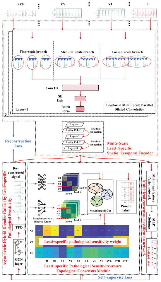
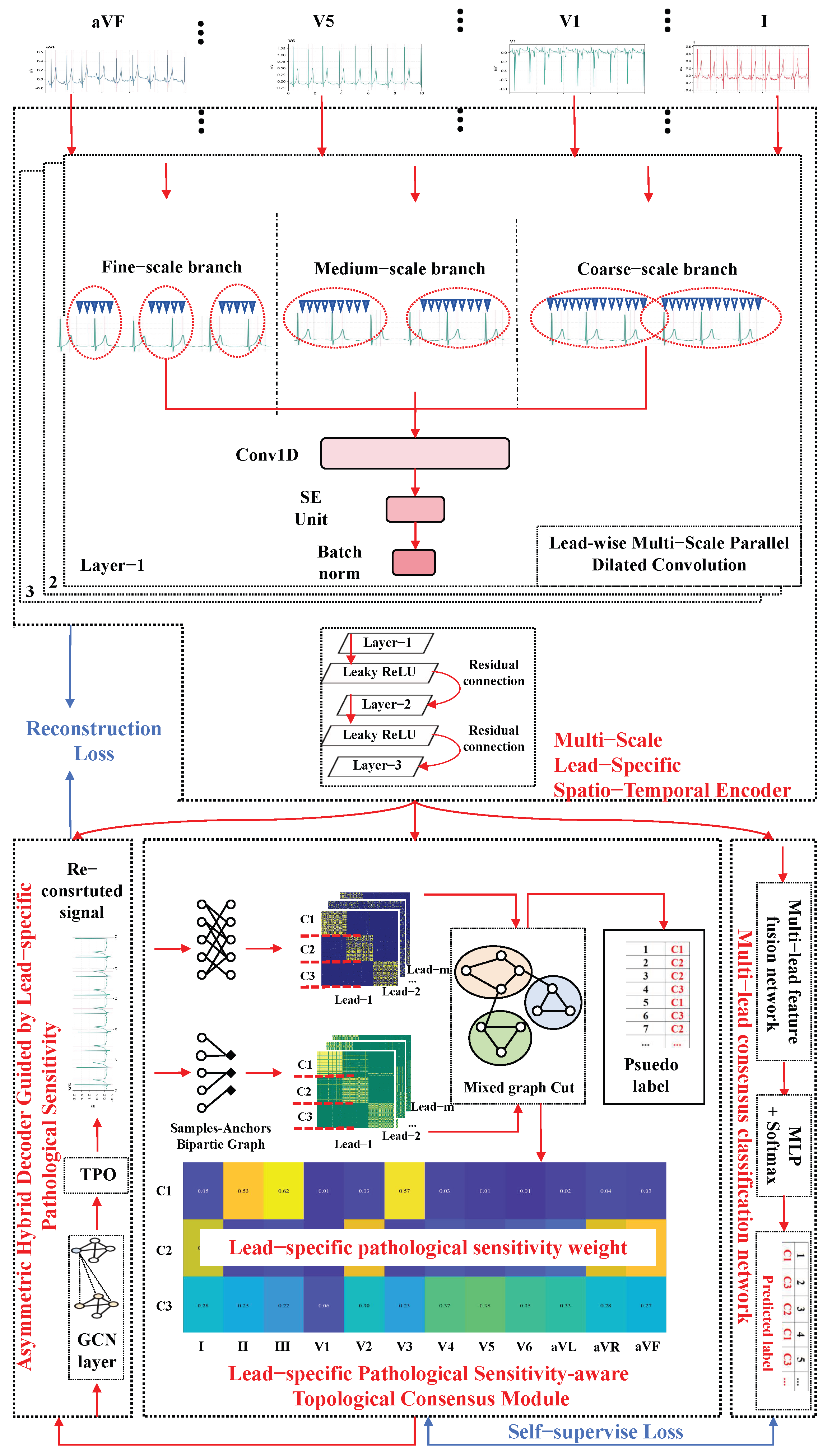
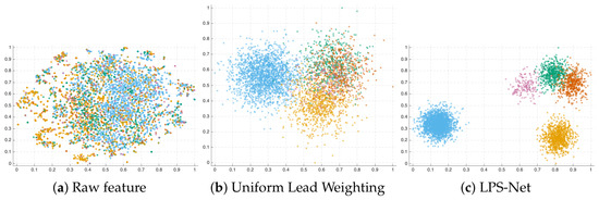
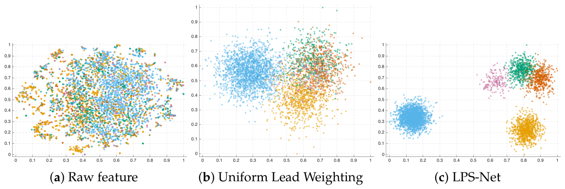
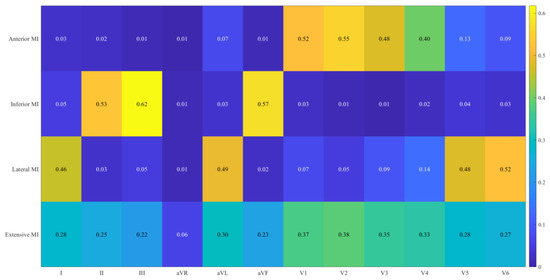
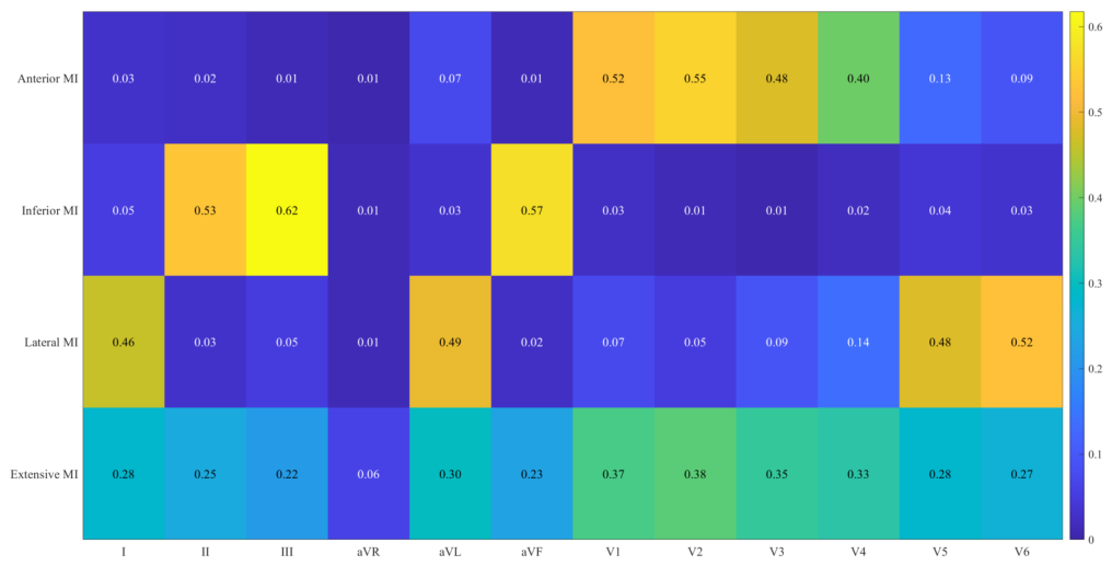

Disclaimer/Publisher’s Note: The statements, opinions and data contained in all publications are solely those of the individual author(s) and contributor(s) and not of MDPI and/or the editor(s). MDPI and/or the editor(s) disclaim responsibility for any injury to people or property resulting from any ideas, methods, instructions or products referred to in the content. |
© 2026 by the authors. Licensee MDPI, Basel, Switzerland. This article is an open access article distributed under the terms and conditions of the Creative Commons Attribution (CC BY) license.