


Abstract
The effects of transcutaneous electroacupuncture stimulation (TEAS) on large-scale brain function remain insufficiently characterized. This study employed a graph-theoretical approach to analyze electroencephalogram (EEG) data from 48 healthy participants in the Pilot-6 TEAS study. Participants received sham (0 pps), 2.5 pps, 10 pps, and 80 pps stimulation during baseline, stimulation, and recovery phases. Functional connectivity was assessed using coherence and the weighted phase-lag index, followed by calculation of global and nodal graph measures from thresholded weighted undirected sensor-level networks. Descriptive analysis indicated potential frequency-related differences in EEG network organization. The 2.5 pps condition exhibited the highest average degree, whereas the 80 pps condition demonstrated the highest average clustering coefficient. At 10 pps, sensor-level maps revealed a distinct frontal–central betweenness-centrality pattern. Although 48 participants provided usable EEG data for descriptive analysis, only 3 participants had complete matched graph-metric data for all four stimulation conditions, limiting repeated-measures statistical validation. After correction for multiple comparisons, no statistically significant frequency-related effects were observed, and nodal hub differences were not independently confirmed. Consequently, these patterns should be interpreted as descriptive and exploratory rather than established group-level effects. These findings indicate that graph-theoretical EEG analysis may facilitate the identification of candidate network features for future investigations of TEAS-related brain network organization.
1. Introduction
Transcutaneous electroacupuncture stimulation (TEAS) is a non-invasive neuromodulation method that uses electrical stimulation via the skin at specific peripheral acupuncture stimulation points. TEAS differs from traditional acupuncture in that it permits the stimulation parameters (frequency and intensity) to be controlled, enabling it to be used in quantitative neurophysiological investigations. Neuromodulation techniques have become increasingly popular in recent years because they can modulate brain activity without invasive procedures. Yet, the mechanisms by which peripheral stimulation influences the organization of large-scale brain regions remain poorly understood. In particular, it remains unknown whether and how different TEAS frequencies change brain communication.
EEG is a clinically accessible, temporally precise tool for measuring brain responses to neuromodulation. EEG records neural activity across many scales on the scalp, enabling it to detect fast oscillatory changes in the brain’s dynamics under stimulation. Studies on acupuncture stimulation have demonstrated that peripheral stimulation can modulate the power and functional connectivity of the human brain in the spectral domain [1]. There are other lines of evidence that suggest stimulation of acupoints may affect functional networks in the brain, not just in the local area [2]. The results support the notion that TEAS should be studied from both a channel-wise and a spectral EEG-descriptor perspective, as well as a network-level perspective on brain communication.
In traditional EEG analysis, the focus of many neuromodulation studies is on the distribution of the power spectrum, the activity at a specific frequency, or the changes at a specific channel. These are helpful but offer little insight into the coordinated interactions among various regions of the brain. Neuromodulation is emerging as a network-level process; stimulation can influence functional integration, segregation, synchronization, and hub organization in distributed neural circuits. Thus, a framework that can model the brain as a structured network of activity, which is provided by EEG, is necessary for understanding brain reorganization under stimulation. Graph theory offers such a system, where the brain is modeled as a graph of nodes and edges. One example of EEG-based functional brain networks is to use scalp electrodes or reconstructed brain regions as nodes and the functional connectivity values between pairs of signals as edges. This mapping enables the conversion of multi-channel EEG recording into graph-structured data.
Local clustering, global efficiency, characteristic path length, modularity, small-world organization, and nodal centrality are then measurable using graph-theoretic metrics, which can provide complementary measures of network topology beyond those discussed above [3,4]. These measures convey meaningful information about the possible distribution, integration, and control of information within the brain network. There are a number of neuromodulation contexts, such as graph-theoretical EEG analysis, where its value has already been demonstrated. In epilepsy, VNS has been found to impact the connectivity and graph-theoretical network measures of the EEG in drug-resistant individuals [5]. Moreover, network-guided models of epilepsy neuromodulation suggest that therapeutic effects are not limited to localized regions of the brain but involve distributed reorganization of brain networks [6,7]. In focal epilepsy, responsive neurostimulation has been associated with long-term reorganization of brain networks [8]. The results suggest that graph metrics could serve as clinically relevant biomarkers of stimulation response. Other stimulation modalities have also been reported to show similar network-level effects. In patients with minimally conscious state (MCS), deep brain stimulation (DBS) has been shown to alter functional connectivity in EEG [9], and, for disorders of consciousness (DoC), a multi-dimensional EEG assessment was used to evaluate the effects of neuromodulation [10]. Some researchers have also explored the application of transcranial magnetic stimulation (TMS) combined with EEG to analyze changes in functional connectivity induced by TMS using graph-theoretical approaches [11,12,13]. Graph-based EEG analysis has been applied in depression to explore EEG–TMS connectivity and to guide the treatment response to repetitive transcranial magnetic stimulation (rTMS) [14,15]. Moreover, transcranial direct current stimulation (tDCS) studies have revealed that stimulation can change the small-world properties and synchronization of EEG-derived brain networks [16,17]. These studies collectively argue for the use of graph theory as a general approach to analyzing brain network changes resulting from neuromodulation.
Traditional EEG analyses and graph-theoretical analyses offer complementary but different descriptions of neural activity. Spectral power analysis measures the magnitude of oscillatory activity at each electrode location or within specific frequency bands. In contrast, graph-theoretical analysis describes the functional relationships among several EEG channels. Thus, this study does not claim that graph features are better than the traditional EEG features. Rather, it determines whether graph-based representations provide network-level information about the effects of different TEAS stimulation frequencies.
While graph-based EEG analysis is widely used in various neuromodulation techniques, the systematic comparison of different TEAS stimulation frequencies using graph theory remains underdeveloped. The novelty of the methodology used in the present study is not the development of a novel graph algorithm or a novel functional-connectivity estimator. Instead, the value of this work is that it uses existing network-analysis tools to explore an understudied paradigm in TEAS and determine whether unique sensor-level EEG networks can be associated with unique stimulation frequencies.
Multi-channel EEG data were acquired under sham, 2.5 pps, 10 pps, and 80 pps TEAS conditions to build functional connectivity matrices. Global and nodal graph metrics were then used to quantify differences in connectivity, local organization, and sensor-level centrality between stimulation conditions. This analysis was designed to be an exploratory and proof-of-concept evaluation of the ability of graph-based EEG representations to include complementary information regarding the frequency-dependent TEAS effects. The principal contributions of this study are as follows:
- 1.
- We apply an established EEG functional-connectivity and graph-theoretical analysis pipeline to a TEAS dataset containing sham, 2.5 pps, 10 pps, and 80 pps stimulation conditions.
- 2.
- We provide a within-dataset comparison of global and nodal graph-theoretical measures across four TEAS frequencies.
- 3.
- We examine whether stimulation frequency is associated with differences in average degree, clustering, and sensor-level centrality patterns.
- 4.
- We identify candidate frequency-dependent network signatures that can be evaluated in future confirmatory, source-level, and clinical studies.
Thus, the present work should be regarded as an application-oriented extension of existing EEG graph-theoretical techniques for TEAS, not as a methodological innovation. Its utility lies in providing an initial network-level characterization of EEG responses to the various TEAS frequencies as well as methodological and empirical questions for further validation.
2. Related Work
Graph-theoretical analysis is now a key computational method for studying brain connectivity. It represents brain regions or EEG electrodes as nodes and their functional or structural relationships as edges, forming structured networks. This approach enables the use of graph metrics to measure network integration, segregation, centrality, modularity, and communication efficiency. Sporns [3] described graph theory as a central mathematical tool for understanding brain networks, noting that measures like clustering coefficient, path length, efficiency, modularity, and centrality each offer unique insights into brain organization. Farahani et al. [4] also reviewed the use of graph theory in human brain connectivity studies and stressed its value for interpreting functional connectivity across various neurophysiological and clinical settings.
One of the key strengths of graph theory in EEG study is that it captures time-varying activity across many scalp locations. Common approaches to traditional EEG analysis include measuring spectral power, event-related activity, or comparing channel-wise activity. These methods are informative, but they do not adequately represent the interactions of distributed brain regions as a coordinated system. The problem is addressed by functional connectivity analysis, which estimates the statistical or phase connectivity between EEG signals. Adjacency matrices can be used to represent these relationships, and thus, the EEG data can be described as a functional brain network. This allows the investigation of local clustering, global information transfer, hub dominance, and network reorganization. These properties are relevant to studies on neuromodulation, as stimulation can modulate not only local activity but also large-scale brain communication.
EEG connectivity and network topology have previously been shown to change following neuromodulation. For instance, vagus nerve stimulation (VNS) has been evaluated by applying EEG graph-theoretical measures in drug-resistant epilepsy. Lanzone et al. [5] found that VNS cycles changed the EEG connectivity patterns, which was consistent with the notion that stimulation affects distributed brain networks. Piper et al. [7] also proposed a network-guided approach to understanding epilepsy neuromodulation, in which therapeutic effects rely on interactions between stimulation targets and the brain’s pathological networks. Likewise, Vetkas et al. [6] noted that connectomics and graph theory may be useful to identify neural networks relevant to the neuromodulation of epilepsy. Long-term network reorganization has been shown to be associated with the outcome of responsive neurostimulation for focal epilepsy, which indicates that graph-based biomarkers can also provide clinically relevant information about treatment response [8].
Other areas of application for graph-theoretical EEG analysis include deep-brain stimulation (DBS) and disorders of consciousness. DBS has been shown to enhance functional connectivity in EEG networks in patients in the minimally conscious state by Dang et al. [9], suggesting that stimulation may have a beneficial effect on large-scale neural coordination. Multi-dimensional EEG assessment was employed to quantify neuromodulation effects in disorders of consciousness, and network-level EEG measures were also shown to be important [10]. These findings imply that stimulus-related recovery or state transitions can be observed in distributed connectivity patterns rather than in isolated signal changes. Thus, the network-based EEG analysis can offer a more comprehensive picture of the modulation of brain state evoked by stimulation.
Further evidence that graph-based EEG measures can capture network changes induced by stimulation comes from transcranial magnetic stimulation (TMS) and repetitive TMS (rTMS) studies. To investigate the propagation of effects through organized brain networks, Amico et al. [11] combined TMS/EEG with diffusion MRI. Siviero et al. (2023) [12] performed TMS–EEG connectivity analysis, and they reported hemispheric differences after occipital stimulation. Recently, Fernández-Linsenbarth et al. [13] studied the modulation of functional connectivity in healthy controls due to TMS, using a graph-theoretical EEG approach. In clinical populations, Olejarczyk et al. [14] investigated the graph-theoretic indices of EEG–TMS connectivity in depression patients, and Nobakhsh et al. [15] applied graph-based EEG analysis to predict rTMS treatment responses for patients with MDD. The findings from these studies indicate that graph metrics can be used not only as network organizational descriptors but also as predictive markers of response to neuromodulation.
Another technique that has been investigated with graph-theoretical EEG techniques is transcranial direct current stimulation (tDCS). Mancini et al. [16] investigated cortical synchronization during tDCS and demonstrated that a graph-theoretical approach can detect changes in the network’s interaction patterns induced by tDCS. However, Vecchio et al. [17] reported that tDCS had a short-term effect on small-world brain connectivity, suggesting temporal modulation of the ratio of local clustering to long-range communication efficiency. The significance of these studies lies in the fact that a small-world organization is an efficient network architecture that enables local specialized processing while also allowing for global integration of communication. Thus, alterations of small-worldness, clustering, and efficiency serve as valuable measures of the effects of neuromodulation on brain network topology.
Studies on acupuncture-related stimulation are more relevant to the present work, particularly those involving stimulation of peripheral acupoints, which are closely related to TEAS. To date, Yu et al. [1] demonstrated that acupuncture stimulation could change the spectral power and functional connectivity in the human brain, which indicated that peripheral stimulation can affect distributed neural activity. In the study of magnetic stimulation of acupoints, Xing et al. [2] built and analyzed brain functional networks using graph theory, demonstrating the applicability of network analysis to acupoint stimulation paradigms. Another non-invasive stimulation technique, pre-frontal transcranial photobiomodulation, was also found to have the ability to modulate brain power topography and network topology by Shahdadian et al. [18]. Taken together, these studies propose that non-invasive stimulation methods can generate network-level changes detectable by graph-based EEG analysis.
Recent advances in computational neuroscience and machine learning are another indication of the use of graph-based EEG representations. Liu et al. [19] introduced a multi-frequency EEG and multi-functional connectivity graph convolutional network (CNN) to classify neurological diseases, such as Alzheimer’s disease, demonstrating that the frequency-resolved graph representation has the potential to enhance neurological classification accuracy. Díaz-Montiel et al. [20] explored optimal graph representations and neural networks to tackle multi-channel time-series data in seizure phase classification. The studies presented show that graph-structured EEG features can serve as a basis for predictive modeling, classification, and intelligent diagnostic systems. Thus, graph-theoretical analysis can be used not only to describe brain networks but also to build future computational models for brain-state prediction and assessment of stimulation response.
In addition to EEG neuromodulation, graph-theoretical approaches have been widely used in clinical neuroscience and brain network studies. In neurosurgery, graph metrics have been used to characterize the brain’s eloquent networks and to perform network-based analyses of surgical risk [21,22]. These methods have been extended to brain tumor patients, in which graph analysis has been used to characterize changes in functional and structural network organization [23]. The graph-based brain network analysis has also recently been applied to other disorders, such as systemic lupus erythematosus (SLE) [24], pre-clinical neurodegeneration [25], Parkinson’s disease [26], and speech-processing disorders [27], demonstrating that graph metrics can reflect disease-related changes in the patterns of brain communication. While not specifically targeting TEAS, these studies offer support to the overall clinical relevance of graph theory as a tool for detecting clinically important changes in brain network topology. In a neuromodulation-related study, Morrison et al. [28] demonstrated that VNS could produce dose-dependent effects on EEG power and synchronization, and Okoroafor et al. [29] presented an overview of neurophysiological biomarkers for invasive neuromodulation therapy for epilepsy. Shao et al. [30] also showed that the network synchrony induced by stimulation might exhibit a non-linear dose–response pattern in tDCS modeling. All of these studies resonate with the notion that stimulation parameters can have measurable and complex effects on the brain network organization.
Graph-theoretical methods are also becoming increasingly relevant in broader computational and biomedical informatics, where complex biological and clinical systems can be represented as interconnected networks. Mishra [31] discussed the integration of graph theory, network analysis, and artificial intelligence in intelligent healthcare infrastructures, while Chen et al. [32] demonstrated the use of dynamic graph-attention mechanisms with clinical knowledge graphs for diagnostic modeling. Although these studies do not directly investigate EEG-based neuromodulation, they illustrate the broader information-science value of graph-based representations for modeling complex biomedical systems. This computational perspective is relevant to the present study, in which multi-channel EEG connectivity is transformed into graph representations from which interpretable network-level features are derived.
While these studies demonstrate the utility of graph-theoretical EEG analysis across a variety of neuromodulation modalities, the frequency-dependent modulation of EEG-derived functional brain networks by TEAS remains underexplored. Previous studies have demonstrated that stimulation can induce changes in EEG connectivity, small-world organization, and hub structure, but relatively little work has directly compared the effects of various TEAS stimulation frequencies on the formation of distinct network states. This gap is critical because the stimulation frequency is one of the parameters that can determine whether stronger local clustering, a change in the organization of the brain’s hubs, or greater integration occurs. The current study aims to fill this gap by examining EEG data obtained under the sham, 2.5 pps, 10 pps, and 80 pps TEAS conditions using graph-theoretical analysis as demonstrated in Table 1. It seeks to examine whether TEAS frequency may be associated with differences in functional brain network organization and to identify candidate EEG graph features for future validation.
Table 1.
Summary of related studies using EEG connectivity, graph-theoretical analysis, or network-based neuromodulation frameworks.
Previous studies have found evidence that peripheral acupuncture or acupoint stimulation changes EEG activity and alters functional connectivity. Both Yu et al. [1] and Xing et al. [2] showed alterations in functional connectivity and spectral power during acupuncture stimulation and magnetic stimulation of acupoints, respectively. Connectivity and network analysis have been used to investigate brain responses to stimulation, as supported by these studies. However, their results cannot be compared numerically as in the present study due to variations in stimulation modality, EEG acquisition, connectivity estimation, graph construction, frequency bands, and reported outcome measures. So, the present results are not compared directly with earlier ones but in the context of general trends.
Ke et al. [33] presented a similar representation learning method using an unsupervised deep frequency-channel attention factorization to perform non-linear feature extraction in fMRI data. They integrate non-linear processing with a neural network, attention mechanisms, and tensor factorization to project high-dimensional neuroimaging data into discriminative features that improve Parkinson’s disease identification and help interpret functional connectivity. This study tackles a related representation problem differently. While fMRI data learn a latent feature space, multi-channel EEG signals are converted into functional-connectivity matrices and visualized as graphs. These high-dimensional matrices are summarized into interpretable measures of local connectivity, network organization, and sensor-level centrality using graph-theoretical metrics. Thus, both methods complement each other in mapping complex neural data onto compact representations of functional brain states. Unlike deep non-linear feature learning and classification, the current method emphasizes interpretability and descriptive network analysis.
A variety of studies have demonstrated that graph-theoretic EEG analysis can reveal changes in functional connectivity, network integration, segregation, and hub organization during the stimulation of different neuromodulation techniques, including VNS, DBS, TMS, rTMS, and tDCS. Studies on acupuncture have also shown that peripheral stimulation can modify the EEG spectral activity and functional connectivity. Few studies, however, have directly compared the EEG graph measures obtained from different frequencies of the TEAS stimulation in the same subjects.
This study addressed this application-specific gap by comparing the sham condition with 2.5 pps, 10 pps, and 80 pps TEAS, using well-defined graph-theoretical and functional-connectivity procedures. This study does not propose a new graph-theory-based methodology. Rather, it examines whether existing network measures can provide an interpretable description of TEAS-related EEG differences as a function of frequency. Hence, in this work, previously known graph analysis techniques are applied to a relatively under-explored neuromodulation setting.
3. Materials and Methods
Using an EEG-based graph-theoretical framework, this study examined the reorganization of the brain networks during TEAS at various frequencies. The methodological pipeline involved the following steps: EEG data acquisition, pre-processing, segmentation by experimental phase, estimation of functional connectivity, graph construction, extraction of graph metrics, and statistical comparison of graphs across different stimulation frequencies.
Figure 1 shows the full workflow for this study. The analysis starts with the Pilot-6 TEAS EEG dataset, which includes multi-channel EEG recordings collected under sham, 2.5 pps, 10 pps, and 80 pps stimulation. After collecting the data, we pre-processed the EEG signals to reduce noise, remove artifacts, and create clean epochs for analysis. We then chose representative epochs from the baseline, stimulation, and recovery phases. Next, we estimated functional connectivity between all EEG channel pairs to create condition-specific connectivity matrices. We converted these matrices into weighted undirected graphs, with each EEG channel as a node and each connection as an edge. We extracted graph-theoretical metrics to measure global network organization and nodal hub properties. Finally, we compared results across stimulation frequencies to describe possible frequency-related patterns in EEG network organization.
Figure 1.
Methodological workflow of the EEG graph-theoretical analysis. The pipeline begins with TEAS EEG data acquisition under sham, 2.5 pps, 10 pps, and 80 pps stimulation conditions. EEG signals are pre-processed, segmented into baseline, stimulation, and recovery phases, and transformed into functional connectivity matrices. These matrices are then represented as weighted undirected graphs, from which global and nodal graph metrics are extracted. Statistical and descriptive analyses are finally performed to examine possible frequency-related patterns in EEG network organization.
3.1. Dataset and Experimental Design
The Pilot-6 TEAS EEG dataset was obtained from healthy adult volunteers. A total of 48 participants (aged 22 to 65 years) participated in EEG recordings. The total number of subjects included healthy volunteers with no reported neurological disorder at the time of recording. The EEG activity was recorded for four experimental conditions: sham stimulation, 2.5 pulses per second (pps), 10 pps, and 80 pps of TEAS stimulation. The three active stimulation conditions were used to investigate the impact of stimulation frequency on EEG-derived functional brain networks, with the sham condition serving as the control.
The experimental design was a repeated-measures design: the same participants were stimulated across all conditions, and EEG was recorded at various temporal phases. In this graph-theoretical analysis, three representative EEG segments were selected from the baseline, stimulation, and post-stimulation recovery phases. These stages enabled comparison of the brain network’s organization before, during, and after exposure to TEAS. For the present analysis, special attention will be given to differences in frequency across the sham (no stimulation), 2.5 pps, 10 pps, and 80 pps conditions.
3.2. TEAS Setup and Stimulation Conditions
A charge-balanced Equinox E-T388 electrical stimulator (Equinox International, St Peter Port, Guernsey, UK) was used to administer TEAS. Surface electrodes stimulated both hands bilaterally. One electrode was placed on the dorsum of the hand over LI4 (Hegu) between the first and second metacarpal bones. The second electrode was placed over the ulnar border of the same hand. The electrical current flowed only between the electrodes on each hand, not through the arm or torso.
All participants underwent four experimental sessions with sham, 2.5 pps, 10 pps, and 80 pps conditions. The three active conditions used charge-balanced, alternating monophasic pulses at 2.5, 10, and 80 pulses per second. The output amplitude was adjusted individually for each active session until the participant reported a strong but comfortable sensation. No values were given for current amplitude or pulse width in the original experiments. TEAS was run for 20 min, divided into four 5 min stimulation phases. Halfway through, there was a brief break for participants to sit and complete study questionnaires.
In the original protocol, the device frequency was set at 160 Hz, and the output amplitude was kept at zero. The stimulator was not disabled, but no intended stimulation current was delivered, and the stimulator’s indicator was flashing. The participant was asked to imagine that the operator increased the amplitude they were observing. This is termed 0 pps sham in the present manuscript to conform with the graph-analysis comparisons and does not mean that the device is set to zero internal frequency setting. Rather, the output amplitude is set to zero.
The stimulation conditions were presented in a semi-randomized balanced order. There was a washout period of at least one week between conditions. The sham procedure was designed to blind participants to the lack of actual stimulation, but some experienced occasional sensations during sham. Blinding was thus potentially incomplete and not formally evaluated. The active stimulation was adjusted to a strong but comfortable perceived intensity. However, the experimental evidence does not mention a standardized scale for perceived intensity or rate the intensity of the conditions.
3.3. Ethical Approval and Consent
EEG data were recorded at the University of Hertfordshire in the UK. This study was approved by the ethics committee (protocol HSK/SF/UH/00124, 17 August 2015). The study followed the principles of the Declaration of Helsinki. Written informed consent was obtained from all participants before data collection. For the present study, the data were made anonymous prior to analysis.
3.4. EEG Acquisition
A total of 19 scalp electrodes were positioned according to the International 10–20 system to record EEG signals. Electro-Cap International caps were selected according to each participant’s head size. EEG data were recorded using a Mitsar EEG-202 amplifier (Mitsar, St. Petersburg, Russia) and WinEEG software (version 2.91.54). The original recording reference consisted of linked-ear electrodes, while the ground electrode was positioned anterior to Fz. The EEG signals were sampled at 500 Hz.
EEG recordings were obtained for 40 min during each experimental session and were divided into eight consecutive 5 min blocks. These included a 5 min baseline period, four stimulation blocks corresponding to 20 min of TEAS, and three post-stimulation blocks corresponding to 15 min after stimulation. During the recordings, participants were seated comfortably with both forearms supported. They were instructed to keep their eyes open and maintain a relaxed visual focus on an object positioned in front of them to minimize eye-movement artifacts.
The EEG cap and physiological sensors remained in place throughout the experimental session. The complete sessions typically lasted approximately 60–90 min, including participant preparation, questionnaire completion, stimulation, EEG recording, and post-recording procedures.
3.5. EEG Pre-Processing
The EEG recordings were acquired in WinEEG format and subsequently exported to the European Data Format (EDF). Each experimental session was divided into eight consecutive 5 min files, consisting of one baseline file, four stimulation files, and three post-stimulation files.
The EEG signals were band-pass filtered between 0.5 and 45 Hz using second-order Butterworth filters implemented with the MATLAB, R2022a (The MathWorks, Inc., Natick, MA, USA) butter and filtfilt functions. Because the recordings were obtained in the United Kingdom, where the mains electricity frequency is 50 Hz, an additional notch filter between 49 and 51 Hz was applied to suppress power-line interference.
Independent component analysis (ICA) using the extended Infomax algorithm was applied to identify non-neural components. Artifact-related components were evaluated using the Multiple Artifact Rejection Algorithm (MARA) and ICLabel within EEGLAB (EEGLAB13_4). Components associated with ocular, muscular, or other non-neural activity were removed before subsequent analysis.
The TrimOutlier EEGLAB plug-in was used to remove data points exceeding an amplitude threshold of standard deviations from the mean across all EEG channels. Following artifact removal, the EEG recordings were re-referenced using the CSD Toolbox with a surface-Laplacian local average reference.
Recordings were excluded if they contained missing data, poor signal quality, inconsistent sampling rates, or incomplete experimental sessions. After quality-control procedures, EEG data from 48 participants remained available for analysis.
3.6. Experimental Phase Selection
EEG epochs were extracted from three important phases for each participant and stimulation condition:
- 1.
- Pre-stimulation phase: EEG recorded prior to the stimulation onset.
- 2.
- Stimulation phase: EEG recorded during TEAS exposure.
- 3.
- Post-stimulation phase: EEG that was recorded after stimulation.
In this study, these phases were used to investigate changes in functional brain network organization over time following TEAS. The primary frequency-dependent comparison was between sham and 2.5 pps, 10 pps, and 80 pps conditions.
3.7. Spectral Decomposition
Functional connectivity was examined separately within the alpha, beta, and gamma EEG frequency bands rather than across the broadband EEG signal. The frequency ranges were alpha, 8–13 Hz; beta, 14–30 Hz; and gamma, 30–45 Hz. Each pre-processed EEG segment was transformed into the frequency domain using Welch’s method with a 2 s window and 50% overlap. Frequency-specific spectral estimates were obtained for each participant, stimulation condition, experimental phase, and EEG frequency band. The temporal phases included the 5 min pre-stimulation baseline, four 5 min stimulation slots, and three 5 min post-stimulation slots. Connectivity was evaluated separately across pre, stim, and post phases.
3.8. Functional Connectivity Estimation
Functional connectivity was estimated by computing pairwise relationships between EEG channels. The connectivity matrix for each participant, condition, and phase was computed for all EEG channel pairs, yielding a matrix. Each matrix element represented the degree of functional association between EEG channels.
For each participant, stimulation condition, and experimental phase, the functional connectivity matrix was defined as
where represents the functional connectivity between EEG channels i and j. Self-connections were excluded by setting
Because
the connectivity matrix was symmetric and was represented as an undirected weighted graph.
To estimate functional connectivity, magnitude-squared coherence and the weighted Phase-Lag Index (wPLI) were computed. Coherence quantifies linear frequency-domain synchronization between EEG signals but is susceptible to zero-lag correlations from volume conduction and common-source activity. Therefore, wPLI was used because it emphasizes consistent non-zero phase-lag interactions while reducing the influence of instantaneous coupling and common-reference effects. The two estimators provide complementary information: coherence reflects overall synchronization, and wPLI offers a more conservative estimate of physiologically meaningful phase relationships. Since both measures were calculated from scalp EEG recordings, all connectivity matrices were interpreted as sensor-level functional connectivity rather than direct anatomical connectivity.
3.9. Graph Construction and Thresholding
The functional connectivity matrices were visualized as weighted undirected graphs, with each EEG electrode represented as a node and edge weights indicating the strength of connections. Each connectivity matrix was thresholded proportionally to minimize the effects of weak or possibly spurious connections while retaining a similar network density for each connectivity condition. In particular, the best 30% of weighted connections were kept, while the rest were discarded. Because this ensures the same network density across participants and conditions, we chose a proportional threshold and made meaningful comparisons of graph topology regardless of the number of edges retained. The thresholded weighted adjacency matrix was defined as:
where denotes the normalized functional connectivity weight between electrodes i and j, and T represents the proportional threshold corresponding to the strongest 30% of connections.
Weighted sparse networks were then created, and, subsequently, graph-theoretical metrics were computed. The following analyses focused on measures that primarily reflect local topology and network organization, such as clustering coefficient, modularity, spectral radius, and nodal centrality measures, which provide more information about the organization of these networks under the assumption of a fixed network-density graph construction.
3.10. Threshold Sensitivity
Complementary robustness analyses were performed to check if the results in the graph-theoretical analyses were methodologically dependent. Each connectivity matrix used the most connected 30% of the primary graph. Main global graph metrics were then recomputed on proportional thresholds of 20%, 30%, and 40%, respectively, which correspond to more or less sparse, primary, and denser network constructions.
Two measures of functional connectivity, the magnitude-squared coherence and the weighted phase-lag index, were used. While the weighted phase-lag index favors similar non-zero phase relationships and minimizes the impact of instantaneous coupling due to volume conduction, the coherence measures amplitude–phase synchronization in the frequency domain. Both estimators were first normalized, then thresholded proportionally, and finally used to compute the graph metric.
The temporal development of network organization was investigated using graph measures in the pre-stimulation, stimulation, and post-stimulation phases separately. The key global metrics included were clustering coefficient, modularity, spectral radius, and Laplacian entropy. Nodal measures used were degree, strength, betweenness centrality, and eigenvector centrality.
Means and standard deviations were used to illustrate participant-level variability. The data under the sham, 2.5 pps, 10 pps, and 80 pps condition(s) were obtained in the same participants by repeated-measures inferential analysis. Matched, graph-metric observations were attempted for the tested combinations of only three participants. Thus, the conclusions of individual response heterogeneity and formal statistical results should be considered with caution.
3.11. Graph-Theoretical Metrics
Global network organization and the relative importance of individual EEG sensors were quantified by graph-theoretical measures. Metrics used globally were the clustering coefficient, modularity, spectral radius, and Laplacian entropy.
Nodes were locally organized into groups by clustering coefficient, which indicated the tendency of neighboring nodes to be interconnected. Modularity measures how well the network could be partitioned into communities with higher internal cohesion than external cohesiveness. The overall coupling structure of the network was described by the spectral radius, defined as the largest eigenvalue of the weighted adjacency matrix. Laplacian entropy summarized the complexity and distribution of connectivity in the graph.
The node metrics used were degree, strength, betweenness centrality, and eigenvector centrality. Degree was the number of retained connections that each EEG sensor was connected with, while strength was the total of all connections’ weights. Betweenness centrality was used to determine the degree to which a sensor was in the middle, or between, other sensors in the network. Eigenvector centrality gave higher weight to sensors that were connected to other sensors with a high centrality.
Average network degree and average network density were not considered as condition-dependent outcomes since proportional thresholding kept the overall number of network connections. Nodal degree was only kept to describe the spatial distribution of connections across the EEG sensors.
These metrics, such as characteristic path length, global efficiency, and small-worldness, were not used in the updated analysis because they required a valid transformation of connectivity weights into distances. The proportional-thresholding procedure was used to control density, so density itself was not analyzed as a graph outcome.
3.12. Hub Identification
Nodal graph metrics, such as betweenness centrality and node strength, were used to analyze hub organization. The relatively high centrality values of the channels were selected as candidate hub nodes. These hubs were then compared across different stimulation conditions to determine whether stimulus frequency altered the spatial location of influential network nodes.
A particular focus of the analysis was whether 10 pps stimulation led to greater frontal–central hub dominance and whether 80 pps stimulation led to more localized or fragmented hub patterns. This network-level analysis was conducted at a hub level to facilitate the interpretation of frequency-dependent network reorganization.
3.13. Statistical Analysis
Observations were recorded for each participant under the sham (0 pps), 2.5 pps, 10 pps, and 80 pps stimulation conditions. Therefore, comparisons among stimulation frequencies were analyzed using a repeated-measures approach.
The Friedman test was used to assess differences among the four stimulation conditions for each connectivity estimator, EEG frequency band, experimental phase, proportional threshold, and graph metric. This non-parametric repeated-measures test was selected because it does not require the observations to follow a normal distribution and allows comparison of more than two related conditions.
Wilcoxon signed-rank tests were used to compare paired stimulation conditions where follow-up analyses were required. The Benjamini–Hochberg false discovery rate procedure was applied to adjust the resulting p-values. Kendall’s W was reported as the effect size for the Friedman test, whereas the rank-biserial correlation was used as the effect size for Wilcoxon signed-rank comparisons. Descriptive data were expressed as mean ± standard deviation (SD).
A complete-case repeated-measures approach was employed. Only participants with graph-metric values available under all four stimulation conditions were included in each inferential comparison. Although 48 participants had acceptable pre-processed EEG data for data organization and descriptive analysis, only three participants had matched observations across all combinations included in the statistical validation. Consequently, the Friedman tests, Kendall’s W values, and post hoc comparisons were based on . Because of the very small inferential sample size, the statistical findings were considered exploratory rather than confirmatory.
The primary hypothesis was that EEG graph-theoretical metrics would differ among the sham, 2.5 pps, 10 pps, and 80 pps TEAS conditions. Based on previous studies, the analysis also examined whether the 10 pps condition showed a distinct frontal–central centrality pattern and whether the 80 pps condition showed increased local clustering. Since nodal hub differences were not tested independently, these spatial patterns were described rather than interpreted as definitive evidence of changes in network integration or fragmentation.
4. Results
Graph-theoretical analysis revealed descriptive differences in EEG-based functional network organization across the sham, 2.5 pps, 10 pps, and 80 pps TEAS conditions. These patterns were assessed using global graph measures, nodal features, centrality maps, and hub-network visualizations. Because the corrected repeated-measures analyses did not identify statistically significant frequency effects following FDR correction, these results are presented as exploratory network patterns rather than confirmatory evidence for frequency-specific effects.
The results are organized into four analytical categories: (1) descriptive graph-metric summaries derived from the available data, (2) complete-case repeated-measures statistical validation with n = 3, (3) exploratory nodal feature ranking, and (4) descriptive nodal centrality and hub-network visualization. Threshold-sensitivity and robustness analyses are reported separately as methodological checks.
Figure 2, Figure 3, Figure 4 and Figure 5 show the topographic distribution of node degree, clustering coefficient, and betweenness centrality across the standard 10–20 EEG electrode locations. Across all stimulation conditions, node degree remained relatively distributed, with modest increases over frontal and central electrode sites. Clustering coefficient showed localized variation, suggesting differences in local network organization across stimulation frequencies. The most distinct changes were observed in betweenness centrality, where the 10 pps condition showed comparatively stronger frontal–central involvement, while the 80 pps condition showed a more localized and less uniformly distributed pattern.
Figure 2.
Sensor-level topographic distributions of node degree, clustering coefficient, and betweenness centrality under the sham condition.
Figure 3.
Sensor-level topographic distributions of node degree, clustering coefficient, and betweenness centrality under the 2.5 pps TEAS condition.
Figure 4.
Sensor-level topographic distributions of node degree, clustering coefficient, and betweenness centrality under the 10 pps TEAS condition.
Figure 5.
Sensor-level topographic distributions of node degree, clustering coefficient, and betweenness centrality under the 80 pps TEAS condition.
4.1. Descriptive Graph-Metric Summaries Based on Available Data
For the global analysis, we used clustering coefficient, modularity, spectral radius, and Laplacian entropy. We calculated these measures separately for coherence- and wPLI-based networks in the alpha, beta, and gamma bands, as well as during the pre-stimulation, stimulation, and post-stimulation phases.
We used proportional thresholding to build all networks, so network density stayed the same and average degree was set by design. Therefore, we did not use density or average degree to show greater global integration. We treated the nodal results as descriptions of sensor-level patterns. This was especially true because the corrected repeated-measures tests used a limited sample of complete cases.
Table 2 summarizes the descriptive values of the global EEG graph measures across the sham, 2.5 pps, 10 pps, and 80 pps conditions. In summary, the 80 pps condition had the highest average clustering coefficient. The 2.5 pps condition had the highest average degree. For the 10 pps condition, the average degree was higher than in the sham condition but lower than in the 2.5 pps condition.
Table 2.
Descriptive statistics of global EEG graph metrics across TEAS stimulation frequencies based on available observations. Values are reported as mean ± standard deviation and median [interquartile range]. The descriptive sample is distinct from the complete-case repeated-measures inferential sample (n = 3).
However, only three participants had complete matched data for all four stimulation conditions in the corrected repeated-measures analysis. After applying the Benjamini–Hochberg false-discovery-rate correction, none of the tested frequency effects were statistically significant. As a result, the differences in clustering and degree should be seen as descriptive trends, not as confirmed frequency-dependent effects.
4.2. Complete-Case Repeated-Measures Statistical Validation (n = 3)
Although 48 participants provided acceptable pre-processed EEG data for descriptive analyses, only 3 participants had complete matched graph-metric observations across all four stimulation conditions required for repeated-measures statistical validation. As a result, the Friedman tests, Kendall’s W effect sizes, and corresponding post hoc comparisons were conducted with n = 3. Following Benjamini–Hochberg FDR correction, none of the tested frequency effects remained statistically significant. Thus, the differences observed in the descriptive graph measures cannot be interpreted as statistically confirmed group-level frequency effects. The inferential findings should be regarded as exploratory due to the very limited complete-case sample.
4.3. Threshold Sensitivity and Robustness Analysis
To check whether the graph-theoretical patterns depended on the proportional threshold used, graph metrics were recalculated with network densities of 20%, 30%, and 40%. The descriptive trends were similar across the thresholds examined. Specifically, the relative differences among the stimulation conditions were maintained, with some graph metrics also changing with network density.
As expected, the higher the proportional threshold, the denser the weighted network became, and its numerical measures (clustering, modularity, and spectral measures) changed accordingly. But the qualitative ordering of the descriptive patterns was generally similar across the examined thresholds. The results indicate that the trends in the descriptions are not only related to the chosen threshold of 30% but that graph-theoretical measures are also dependent on network density. Thus, the results reflect descriptive observations of the network rather than threshold-independent network properties.
We tested robustness using different connectivity estimators, proportional thresholds, experimental phases, and levels of participant completeness. Networks based on coherence and wPLI showed similar, but not identical, patterns. This suggests that the choice of functional-connectivity measure affects the estimated graph organization.
We also examined the main graph measures at proportional densities of 20%, 30%, and 40%. While there were some descriptive differences between stimulation conditions at these thresholds, the absolute metric values changed with network density. Thus, the results should not be seen as fully independent of the chosen threshold.
Some measures varied across the pre-stimulation, stimulation, and post-stimulation phases. In the alpha band, clustering usually increased, modularity tended to decrease, and spectral radius often increased during and after stimulation. These patterns are exploratory and were not confirmed as lasting effects, as we pre-processed EEG data from 48 participants for descriptive analysis. Still, only three had complete matched graph-metric data for all four conditions needed for repeated-measures validation. After FDR correction, no frequency-related effects were significant. As a result, all condition-related graph differences are considered exploratory and need to be confirmed with a larger, more complete dataset.
4.4. Exploratory Nodal Feature Ranking
An exploratory nodal feature-ranking analysis was conducted to identify graph features that exhibited greater differentiation among the sham, 2.5 pps, 10 pps, and 80 pps conditions. The candidate features included electrode-level node degree, clustering coefficient, and betweenness centrality. All features were standardized, and those with low variance were removed. ANOVA F-scores were applied for univariate ranking, followed by recursive feature elimination using a linear support-vector classifier as the internal estimator. The support-vector classifier was used solely for feature ranking; no predictive classification performance was evaluated.
The ANOVA F-scores in Table 3 show the ratio of variability between conditions to variability within each condition for every feature. A higher F-score means the feature better separates the four TEAS conditions compared to the variation within each condition. These scores are not percentages, classification accuracies, or effect sizes. We used them only to rank how well each graph feature could distinguish between conditions.
Table 3.
Top-ranked nodal graph features identified using ANOVA F-scores and recursive feature elimination.
Degree at F7 had the highest ANOVA F-score (41.575), followed by degree at T8 (35.937), clustering at F7 (33.659), clustering at Fp2 (27.731), and degree at C3 (27.418). These results show that the biggest differences between conditions were mainly in degree and clustering measures at frontal, temporal, frontopolar, and central sensors. Features with lower F-scores, like clustering at O2 and F4, contributed less to separating conditions on their own but were kept because they added useful information in the multi-variate feature set. The focus on degree and clustering features matches the feature-selection analysis, which found that connectivity distribution and local network organization were the most informative graph properties. The table reports only the features retained in the final selected subset. In recursive feature elimination, every retained feature is assigned rank 1, whereas eliminated features receive ranks greater than 1. The omitted features with rankings greater than 1 were not included in Table 3. Consequently, the identical RFE values do not mean that all retained features had equal importance. Their relative ordering within the selected subset is represented by the ANOVA F-scores.
We used the ANOVA F-scores to screen and rank features, not as confirmatory hypothesis tests. As a result, we did not use the uncorrected p-values to claim that any single electrode was statistically significant, and we did not make any multiple-comparison inferences from Table 3. The ANOVA F-scores and recursive feature elimination were used to rank and retain comparatively informative nodal graph features. This analysis was intended for exploratory feature ranking rather than evaluation of predictive classification performance. Table 3 shows only the feature-selection results and should not be interpreted as a classifier-performance table.
Overall, the selected features came from frontal, temporal, central, parietal, and occipital sensors. This shows that the information used to distinguish TEAS conditions was spread across the scalp, not limited to one area. The higher scores for F7, T8, Fp2, C3, Fp1, Fp2, F3, and F4 suggest that frontal, temporal, and central network properties contributed most. However, these results only indicate relative feature ranking within the exploratory analysis and should not be interpreted as evidence of cortical activation or statistical significance at individual electrodes.
4.5. Descriptive Nodal Centrality and Hub-Network Visualization
The following nodal centrality and hub-network analyses are descriptive visualizations and were not subjected to corrected electrode-wise repeated-measures statistical testing as shown in Figure 6. They should therefore be interpreted as exploratory spatial patterns rather than statistically confirmed nodal effects. Betweenness centrality was examined to explain the spatial distribution of sensor-level nodes considered potentially influential under stimulation conditions. The 10 pps condition showed relatively greater frontal–central involvement in the descriptive topographic maps than the sham condition. However, differences in node activity were not assessed using electrode-wise repeated-measures statistical tests. Therefore, the pattern should be read as a description of an observation, not as evidence of greater network integration.
Figure 6.
Difference maps of betweenness centrality relative to the sham condition. Positive values indicate increased centrality relative to sham, whereas negative values indicate reduced centrality. Descriptively, the 10 pps condition shows the largest frontal–central increase, whereas the 80 pps condition shows a more localized pattern of change.
The 80 pps condition had a sparser distribution of betweenness centrality with less centrality in localized locations. The present analysis did not statistically test for a significant increase in network fragmentation or segregation. The only quantitative evidence for 80 pps is a higher average clustering coefficient, suggesting more organization or tighter cliques in the local network but not necessarily network fragmentation.
Descriptive analysis indicated that the average degree was highest in the 2.5 pps condition, while the average clustering coefficient reached its maximum in the 80 pps condition. The 10 pps condition exhibited a distinct frontal–central centrality pattern in the descriptive maps. However, these condition-related differences were not statistically significant in the complete-case repeated-measures analysis (n = 3) following FDR correction and should be regarded as exploratory observations.
The present findings support that EEG graph organization may differ between TEAS frequencies. They cannot definitively state that 10 pps yields the best network integration or that 80 pps causes network fragmentation statistically.
We examined thresholded hub-network visualizations to describe how prominent sensor-level connections were organized across the TEAS conditions. As shown in Figure 7, Figure 8, Figure 9 and Figure 10, the sham condition had a distributed network pattern without a clear dominant hub. The 2.5 pps condition showed changes mainly in the frontal and central electrode sites.
Figure 7.
Thresholded sensor-level hub network under the sham condition. Nodes represent EEG electrodes according to the standard 10–20 system, with alphanumeric labels indicating electrode positions. Connecting lines represent functional connections retained after network thresholding, while colors visually distinguish the displayed network elements. The figure provides a descriptive visualization of network organization and does not indicate statistically significant nodal differences.
Figure 8.
Thresholded sensor-level hub network under the 2.5 pps stimulation condition. Nodes represent EEG electrodes according to the standard 10–20 system, with alphanumeric labels indicating electrode positions. Connecting lines represent functional connections retained after network thresholding, while colors visually distinguish the displayed network elements. The figure provides a descriptive visualization of network organization and does not indicate statistically significant nodal differences.
Figure 9.
Thresholded sensor-level hub network under the 10 pps stimulation condition. Nodes represent EEG electrodes according to the standard 10–20 system, with alphanumeric labels indicating electrode positions. Connecting lines represent functional connections retained after network thresholding, while colors visually distinguish the displayed network elements. The figure provides a descriptive visualization of network organization and does not indicate statistically significant nodal differences.
Figure 10.
Thresholded sensor-level hub network under the 80 pps stimulation condition. Nodes represent EEG electrodes according to the standard 10–20 system, with alphanumeric labels indicating electrode positions. Connecting lines represent functional connections retained after network thresholding, while colors visually distinguish the displayed network elements. The figure provides a descriptive visualization of network organization and does not indicate statistically significant nodal differences.
The 10 pps condition showed more involvement in the frontal and central areas in the network visualization. However, this pattern was not confirmed by corrected electrode-wise repeated-measures testing and should not be seen as evidence of the strongest global network integration.
The 80 pps condition had a more localized pattern of prominent connections. Still, the visualization alone does not prove more fragmentation or segregation. Its higher average clustering coefficient suggests stronger local organization but does not directly show reduced global communication.
Overall, these hub-network figures show exploratory differences at the sensor level between the stimulation conditions. They are meant to help describe the network organization, not to show statistically confirmed differences in hub dominance, integration, or fragmentation.
4.6. Qualitative Summary of Exploratory Network Patterns
Table 4 summarizes the main quantitative and descriptive EEG graph-theoretical findings across the four TEAS stimulation conditions. The interpretations are based on the statistically tested global graph measures and the descriptive sensor-level centrality maps. The visual hub and centrality patterns were not treated as independently confirmed statistical findings.
Table 4.
Qualitative summary of EEG network organization across TEAS stimulation frequencies.
The sham condition is the reference network state and had the lowest average clustering and a moderate average degree among the four conditions. The 2.5 pps condition had the highest average degree, suggesting more connectivity with nodes overall than the sham condition. The average degree was also higher for the 10 pps condition than for sham but lower than for 2.5 pps. Sensor-level maps showed a characteristic pattern of centrality in the frontal part of the map, but this pattern was not statistically tested at the nodal level. The clustering coefficient is the highest on average under the 80 pps condition, indicating better local network organization. The centrality pattern was more localized in descriptive maps, but, in the present results, there was no adequate statistical proof of the network’s fragmentation or segregation. Overall, the descriptive results suggest possible differences in EEG graph organization across stimulation frequencies; however, these patterns were not statistically confirmed in the limited complete-case repeated-measures analysis and require validation in a larger dataset.
5. Discussion
The present study investigated whether EEG-based functional network organization exhibited distinct descriptive patterns across different TEAS stimulation frequencies. Descriptive analyses indicated variations in average clustering coefficient and average degree among the sham, 2.5 pps, 10 pps, and 80 pps conditions. However, only three participants provided complete matched graph-metric data across all four conditions, limiting the statistical power for repeated-measures validation. None of the frequency effects remained statistically significant following FDR correction. Therefore, these findings should be regarded as primarily descriptive and exploratory. Effect-size estimates from the limited complete-case analysis should be interpreted with caution and should not be considered as evidence for established group-level frequency effects.
The results of the active stimulation conditions were not uniform. The average degree was highest for the 2.5 pps condition, indicating this frequency had the most nodal connections on average. The 80 pps condition had the highest mean clustering coefficient, suggesting a relatively higher level of local network organization. The average degree in the 10 pps condition was between sham and 2.5 pps. Thus, quantitative global measures do not support that 10 pps resulted in the greatest overall network integration.
Under the 10 pps condition, maps of descriptive betweenness-centrality and hub-network revealed a unique frontal–central map. This does not mean all nodes or influential nodes are more connected but rather a reorganization of nodes in the influential domain at the sensor level. To avoid treating electrode-wise hub differences as requiring separate nodal-level tests, the frontal–central pattern should be seen as an exploratory sensor-level check. Similarly, the localized pattern below 80 pps is insufficient to conclude network fragmentation or partition. The strongest quantitative evidence is the greater clustering coefficient, indicating local organization but not necessarily fragmentation.
These findings are best interpreted using the revised graph-construction procedure. The strongest 30% of off-diagonal functional connections were retained using proportional thresholding. Analyses at 20% and 40% densities assessed threshold sensitivity. Thus, network density was controlled for in the design and not an outcome variable. Previously reported density and global-efficiency values of 1.0000 were excluded, as they were inconsistent with the thresholded-network procedure and did not validly indicate condition-related integration. Overall descriptive patterns were similar across thresholds, but absolute graph measure values depended on network density. This confirms the sensitivity of EEG graph interpretation to threshold selection.
While both coherence and wPLI describe functional connectivity, they do not convey overlapping information. Coherence reflects amplitude–phase relationships within the frequency domain and can include zero-lag coupling from “common-source” activity and volume conduction. In contrast, wPLI focuses on consistent non-zero phase-lag relations and minimizes instantaneous coupling effects. Discrepancies between coherence- and wPLI-based results suggest that network response estimation depends on the connectivity measure chosen. Therefore, these results should be interpreted as functional coupling patterns at the sensor level, not anatomical connections between cortical areas.
Selected network measures shifted during the pre-stimulation, stimulation, and post-stimulation periods, as shown in the phase-based analysis. In the alpha band, clustering increased from pre-stimulation to stimulation and post-stimulation phases, while modularity decreased and spectral radius increased. Changes in the beta band were small and less consistent. The descriptive phase-based patterns suggest that EEG network measures may vary across the pre-stimulation, stimulation, and post-stimulation periods. However, these temporal patterns were not statistically confirmed as persistent TEAS-related effects.
Feature-selection analysis at the nodes provided insights into differences in the graph at the individual sensor level. The strongest between-condition separation (highest ANOVA F-scores) was for degree at F7 and clustering at F7 and Fp2. All features received an RFE rank of 1 because Table 3 shows only the final selected features, not those dropped due to higher rank. ANOVA F-scores were used for ranking features, not as individual significance tests. Thus, selected features are not necessarily validated neurophysiological biomarkers but relatively highly ranked features within the exploratory feature-selection analysis.
The results align with previous studies showing that neuromodulation affects not only local neural activity but also distributed functional networks. Changes have been reported in VNS, TMS, rTMS, tDCS, DBS, and acute stimulation studies using acupuncture-related approaches. Previous acupuncture studies reported alterations in EEG spectral power and functional connectivity, with graph analysis applied in acupuncture paradigms. This study advances the literature by using established EEG connectivity and graph-theoretical methods to compare several TEAS frequencies in the same setup. Its contribution lies in applications, not in new graph theory methodology.
Graph analysis should be considered an adjunct and complementary tool to traditional EEG methods, not necessarily superior. Spectral analysis describes oscillatory activity in single electrodes or frequency bands, while graph analysis describes relationships among multiple signals. Microstate, spectral, connectivity, and graph-based approaches reflect different aspects of neural activity. A direct comparison of these feature sets within the same data would be needed to determine if graph features add discriminative information beyond spectral or microstate features.
Transforming EEG into a graph represents neural data from a computational neuroscience perspective. Deep attention-based factorization techniques learn high-dimensional non-linear feature spaces from neuroimaging data, while this approach obtains interpretable, pre-defined topological features from connectivity matrices. Both aim to simplify neural data into meaningful representations, but this approach focuses on network interpretability rather than deep non-linear learning.
The clinical meaning of these results is translational, not confirmatory. This study does not demonstrate treatment efficacy, diagnostic accuracy, or clinically validated biomarkers. However, healthy-participant studies are a crucial first step in establishing physiological features for testing in patient populations. These identified graph patterns could serve as potential network measures for future studies on pain, motor rehabilitation, cognitive self-control, mood disorders, and brain-state monitoring. Clinical insight is not clinical benefit but the potential for the analytical framework and network features to be clinically relevant in the future.
Limitations
This study has some limitations. First, we included only healthy participants and did not collect clinical outcomes, behavioral data, or treatment response information. Therefore, the EEG graph patterns we found should be seen as possible markers for future research, not proven clinical biomarkers. Most importantly, repeated-measures inferential validation was restricted to only three complete cases (n = 3), substantially limiting statistical power and precluding confirmatory group-level conclusions.
Second, using a 19-channel sensor-level EEG setup limited our ability to observe detailed brain activity. While wPLI and Laplacian re-referencing reduced the effects of volume conduction and shared sources, they did not remove them entirely. Thus, the electrode-level patterns we report should not be taken as direct brain connections.
Third, our graph results depended on the connectivity estimator and threshold used. We ran sensitivity analyses at 20%, 30%, and 40% densities, but metric values changed with the threshold. We kept density fixed by design and excluded global efficiency and other shortest-path measures that were not verified from our final interpretation.
Finally, the hub and centrality maps we present are mostly descriptive and were not confirmed with corrected statistical tests for each electrode. We also lacked some details about data collection and stimulation, such as exact impedance limits, pulse width, current amplitude, and the number of usable epochs. Future research should use high-density or source-localized EEG, larger and more complete datasets, repeated measures at the participant level, and corrected nodal testing and include clinical groups with behavioral and treatment outcome data.
6. Conclusions
This study used established methods in functional connectivity and graph theory to examine EEG network organization during sham, 2.5 pps, 10 pps, and 80 pps TEAS conditions. The results showed descriptive differences in average degree and clustering coefficient across stimulation frequencies; however, these differences did not remain statistically significant after FDR correction in the limited complete-case repeated-measures analysis (n = 3). Descriptively, the 2.5 pps condition had the highest average degree, whereas the 80 pps condition had the highest average clustering coefficient. These relative differences were not statistically confirmed in the complete-case repeated-measures analysis. The 10 pps condition showed a higher degree compared to sham and a unique frontal–central betweenness-centrality pattern in the descriptive sensor-level maps. However, this spatial pattern should not be taken as statistically confirmed evidence that 10 pps produced the strongest global integration. Comparing coherence and wPLI, along with the threshold-sensitivity analysis, showed that the estimated network response partly depends on the connectivity estimator and graph-construction parameters. Therefore, these findings should be seen as exploratory sensor-level network patterns, not definitive proof of a single optimal TEAS frequency. Despite these limitations, this study shows that graph-theoretical EEG analysis can turn multi-channel connectivity data into understandable measures of local organization, nodal connectivity, community structure, and sensor-level centrality. These features could serve as candidate network markers for future research in brain-state monitoring, neurorehabilitation, and stimulation response. Their clinical value still needs confirmation through source-level analysis, participant-specific modeling, comparison with standard EEG features, and studies with relevant patient groups.
Author Contributions
Conceptualization, A.S. and D.M.; methodology, A.S., G.P. and D.M.; software, A.S.; validation, R.Z., M.Z., A.U., G.P., S.Y. and D.M.; formal analysis, A.S.; investigation, A.S., S.Y. and D.M.; resources, D.M.; data curation, A.S. and D.M.; writing—original draft preparation, A.S.; writing—review and editing, R.Z., M.Z., A.U., G.P., S.Y. and D.M.; visualization, A.S.; supervision, R.Z., M.Z., A.U., G.P. and D.M.; project administration, A.S. All authors have read and agreed to the published version of the manuscript.
Funding
This research received no external funding.
Institutional Review Board Statement
The University of Hertfordshire ethics review procedure was followed, according to the principles of the Helsinki Declaration, with approval granted by the Health and Human Sciences Ethics Committee with Delegated Authority for the School of Health and Social Work, reference HSK/SF/UH/00124 (17 August, 30 September and 29 October 2015, and 2 June 2016).
Informed Consent Statement
Informed consent was obtained from all subjects involved in the original study. The EEG data used in the present analysis were anonymized before processing. Written informed consent for publication was not required because no identifiable participant information or images are included in this manuscript.
Data Availability Statement
The data analyzed in this study are not publicly available due to ethical and privacy restrictions related to human EEG recordings. Anonymized data may be made available from the corresponding author upon reasonable request and subject to institutional approval.
Acknowledgments
The authors gratefully acknowledge David Mayor and Tony Steffert for their valuable collaboration and for facilitating access to the Pilot-6 EEG dataset used in this study. Their support and contributions to the availability of the dataset are sincerely appreciated.
Conflicts of Interest
The authors declare no conflicts of interest. The funders had no role in the design of the study; in the collection, analyses, or interpretation of data; in the writing of the manuscript; or in the decision to publish the results.
Abbreviations
The following abbreviations are used in this manuscript:
| TEAS | Transcutaneous Electroacupuncture Stimulation |
| EEG | Electroencephalography |
| FC | Functional Connectivity |
| FDR | False Discovery Rate |
| DBS | Deep Brain Stimulation |
| VNS | Vagus Nerve Stimulation |
| TMS | Transcranial Magnetic Stimulation |
| rTMS | Repetitive Transcranial Magnetic Stimulation |
| tDCS | Transcranial Direct Current Stimulation |
| GNN | Graph Neural Network |
| GCN | Graph Convolutional Network |
| ROI | Region of Interest |
References
- Yu, H.; Wu, X.; Cai, L.; Deng, B.; Wang, J. Modulation of spectral power and functional connectivity in human brain by acupuncture stimulation. IEEE Trans. Neural Syst. Rehabil. Eng. 2018, 26, 977–986. [Google Scholar] [CrossRef] [Scilit] [PubMed]
- Xing, Y.; Ma, X.; Geng, Y. Construction and analysis of brain functional network of magnetic stimulation acupoints based on graph theory. Comput. Methods Biomech. Biomed. Eng. Imaging Vis. 2025, 13, 2440073. [Google Scholar] [CrossRef] [Scilit]
- Sporns, O. Graph theory methods: Applications in brain networks. Dialogues Clin. Neurosci. 2018, 20, 111–121. [Google Scholar] [CrossRef] [Scilit] [PubMed]
- Farahani, F.V.; Karwowski, W.; Lighthall, N.R. Application of graph theory for identifying connectivity patterns in human brain networks: A systematic review. Front. Neurosci. 2019, 13, 585. [Google Scholar] [CrossRef] [Scilit] [PubMed]
- Lanzone, J.; Boscarino, M.; Tufo, T.; Di Lorenzo, G.; Ricci, L.; Colicchio, G.; Lazzaro, V.D.; Tombini, M.; Assenza, G. Vagal nerve stimulation cycles alter EEG connectivity in drug-resistant epileptic patients: A study with graph theory metrics. Clin. Neurophysiol. 2022, 142, 59–67. [Google Scholar] [CrossRef] [Scilit] [PubMed]
- Vetkas, A.; Germann, J.; Elias, G.; Loh, A.; Boutet, A.; Yamamoto, K.; Sarica, C.; Samuel, N.; Milano, V.; Fomenko, A.; et al. Identifying the neural network for neuromodulation in epilepsy through connectomics and graphs. Brain Commun. 2022, 4, fcac092. [Google Scholar] [CrossRef] [Scilit] [PubMed]
- Piper, R.J.; Richardson, R.M.; Worrell, G.; Carmichael, D.W.; Baldeweg, T.; Litt, B.; Denison, T.; Tisdall, M.M. Towards network-guided neuromodulation for epilepsy. Brain 2022, 145, 3347–3362. [Google Scholar] [CrossRef] [Scilit] [PubMed]
- Khambhati, A.N.; Shafi, A.; Rao, V.R.; Chang, E.F. Long-term brain network reorganization predicts responsive neurostimulation outcomes for focal epilepsy. Sci. Transl. Med. 2021, 13, eabf6588. [Google Scholar] [CrossRef] [Scilit] [PubMed]
- Dang, Y.; Wang, Y.; Xia, X.; Yang, Y.; Bai, Y.; Zhang, J.; He, J. Deep brain stimulation improves electroencephalogram functional connectivity of patients with minimally conscious state. CNS Neurosci. Ther. 2023, 29, 344–353. [Google Scholar] [CrossRef] [Scilit] [PubMed]
- Zhang, C.; Han, S.; Li, Z.; Wang, X.; Lv, C.; Zou, X.; Zhu, F.; Zhang, K.; Lu, S.; Bie, L.; et al. Multidimensional assessment of electroencephalography in the neuromodulation of disorders of consciousness. Front. Neurosci. 2022, 16, 903703. [Google Scholar] [CrossRef] [Scilit] [PubMed]
- Amico, E.; Bodart, O.; Rosanova, M.; Gosseries, O.; Heine, L.; Van Mierlo, P.; Martial, C.; Massimini, M.; Marinazzo, D.; Laureys, S. Tracking dynamic interactions between structural and functional connectivity: A TMS/EEG-dMRI study. Brain Connect. 2017, 7, 84–97. [Google Scholar] [CrossRef] [Scilit] [PubMed]
- Siviero, I.; Bonfanti, D.; Menegaz, G.; Savazzi, S.; Mazzi, C.; Storti, S.F. Graph analysis of TMS–EEG connectivity reveals hemispheric differences following occipital stimulation. Sensors 2023, 23, 8833. [Google Scholar] [CrossRef] [Scilit] [PubMed]
- Fernández-Linsenbarth, I.; Mijancos-Martínez, G.; Ruiz-Gómez, S.J.; Bachiller, A.; Osorio-Iriarte, E.; Beño-Ruiz-de-la Sierra, R.M.; Arjona-Valladares, A.; Roig-Herrero, A.; Molina, V. Transcranial Magnetic Stimulation-Induced Modulation of Functional Connectivity in Healthy Controls: A TMS–EEG Graph Study. Brain Behav. 2025, 15, e70981. [Google Scholar] [CrossRef] [Scilit] [PubMed]
- Olejarczyk, E.; Jozwik, A.; Valiulis, V.; Dapsys, K.; Gerulskis, G.; Germanavicius, A. Statistical analysis of graph-theoretic indices to study EEG-TMS connectivity in patients with depression. Front. Neuroinform. 2021, 15, 651082. [Google Scholar] [CrossRef] [Scilit] [PubMed]
- Nobakhsh, B.; Shalbaf, A.; Rostami, R.; Kazemi, R. Graph-based Analysis to Predict Repetitive Transcranial Magnetic Stimulation Treatment Response in Patients with Major Depressive Disorder Using EEG Signals. Basic Clin. Neurosci. 2024, 15, 199. [Google Scholar] [CrossRef] [Scilit] [PubMed]
- Mancini, M.; Brignani, D.; Conforto, S.; Mauri, P.; Miniussi, C.; Pellicciari, M.C. Assessing cortical synchronization during transcranial direct current stimulation: A graph-theoretical analysis. NeuroImage 2016, 140, 57–65. [Google Scholar] [CrossRef] [Scilit] [PubMed]
- Vecchio, F.; Di Iorio, R.; Miraglia, F.; Granata, G.; Romanello, R.; Bramanti, P.; Rossini, P.M. Transcranial direct current stimulation generates a transient increase of small-world in brain connectivity: An EEG graph theoretical analysis. Exp. Brain Res. 2018, 236, 1117–1127. [Google Scholar] [CrossRef] [Scilit] [PubMed]
- Shahdadian, S.; Wang, X.; Wanniarachchi, H.; Chaudhari, A.; Truong, N.C.D.; Liu, H. Neuromodulation of brain power topography and network topology by prefrontal transcranial photobiomodulation. J. Neural Eng. 2022, 19, 066013. [Google Scholar] [CrossRef] [Scilit] [PubMed]
- Liu, Y.; An, L.; Yang, H.; Ge, S.S. Multi-frequency EEG and multi-functional connectivity graph convolutional network based detection method of patients with Alzheimer’s disease. Complex Intell. Syst. 2025, 11, 366. [Google Scholar] [CrossRef] [Scilit]
- Díaz-Montiel, A.A.; Zhang, R.; Lankarany, M. Optimal graph representations and neural networks for multichannel time series data in seizure phase classification. Sci. Rep. 2025, 15, 19552. [Google Scholar] [CrossRef] [Scilit] [PubMed]
- Tanglay, O.; Dadario, N.B.; Chong, E.H.; Tang, S.J.; Young, I.M.; Sughrue, M.E. Graph theory measures and their application to neurosurgical eloquence. Cancers 2023, 15, 556. [Google Scholar] [CrossRef] [Scilit] [PubMed]
- Mithani, K.; Suresh, H.; Ibrahim, G.M. Graph theory and modeling of network topology in clinical neurosurgery. In Computational Neurosurgery; Springer: Berlin/Heidelberg, Germany, 2024; pp. 107–122. [Google Scholar]
- Semmel, E.S.; Quadri, T.R.; King, T.Z. Graph theoretical analysis of brain network characteristics in brain tumor patients: A systematic review. Neuropsychol. Rev. 2022, 32, 651–675. [Google Scholar] [CrossRef] [Scilit] [PubMed]
- Yang, Y.; Bai, R.; Liu, S.; Li, S.; Zhao, R.; Wang, X.; Xu, J. Abnormal brain functional networks in systemic lupus erythematosus: A graph theory, network-based statistic and machine learning study. Brain Commun. 2025, 7, fcaf130. [Google Scholar] [CrossRef] [Scilit] [PubMed]
- Ogut, E. Graph-theoretical mapping of cortical and subcortical network alterations in preclinical neurodegeneration. Discov. Neurosci. 2025, 20, 14. [Google Scholar] [CrossRef] [Scilit]
- Siva, K.; Ponnusamy, P.; Chavda, V.; Montemurro, N. The effect of dopaminergic therapy in Parkinson’s disease: A graph theory analysis. Brain Sci. 2025, 15, 370. [Google Scholar] [CrossRef] [Scilit] [PubMed]
- Zhu, H.; Fitzhugh, M.C.; Keator, L.M.; Johnson, L.; Rorden, C.; Bonilha, L.; Rogalsky, C. How can graph theory inform the dual-stream model of speech processing? A resting-state functional magnetic resonance imaging study of stroke and aphasia symptomology. J. Cogn. Neurosci. 2025, 37, 737–766. [Google Scholar] [CrossRef] [Scilit] [PubMed]
- Morrison, E.G.; Danthine, V.; Santalucia, R.; Torres, A.; Cakiroglu, I.; Nonclercq, A.; El Tahry, R. Characterization of vagus nerve stimulation (VNS) dose-dependent effects on EEG power spectrum and synchronization. Biomedicines 2024, 12, 557. [Google Scholar] [CrossRef] [Scilit] [PubMed]
- Okoroafor, F.; Qiang, Z.; Rosenke, S.; Chari, A.; Moeller, F.; Piper, R.J.; Baldeweg, T.; Denison, T.; Tisdall, M. Neurophysiologic Biomarkers of Invasive Neuromodulation Therapy for Epilepsy. Neuromodul. Technol. Neural Interface 2026, 29, 360–375. [Google Scholar] [CrossRef] [Scilit] [PubMed]
- Shao, H.; Gu, G.; Guo, X.; Li, X.; Cui, D. Nonlinear dose-response relationship in tDCS-induced brain network synchrony: A resting-state whole-brain model analysis. Comput. Methods Programs Biomed. 2025, 263, 108675. [Google Scholar] [CrossRef] [Scilit] [PubMed]
- Mishra, P. Design of intelligent healthcare IT infrastructure using graph theory, network analysis, and artificial intelligence. Int. J. Appl. Math. 2025, 38, 2267–2280. [Google Scholar] [CrossRef] [Scilit]
- Chen, D.; Zhang, W.; Ding, Z. Embedding dynamic graph attention mechanism into Clinical Knowledge Graph for enhanced diagnostic accuracy. Expert Syst. Appl. 2025, 267, 126215. [Google Scholar] [CrossRef] [Scilit]
- Ke, H.; Wang, F.; Bi, H.; Ma, H.; Wang, G.; Yin, B. Unsupervised deep frequency-channel attention factorization to non-linear feature extraction: A case study of identification and functional connectivity interpretation of Parkinson’s disease. Expert Syst. Appl. 2024, 243, 122853. [Google Scholar] [CrossRef] [Scilit]
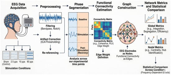
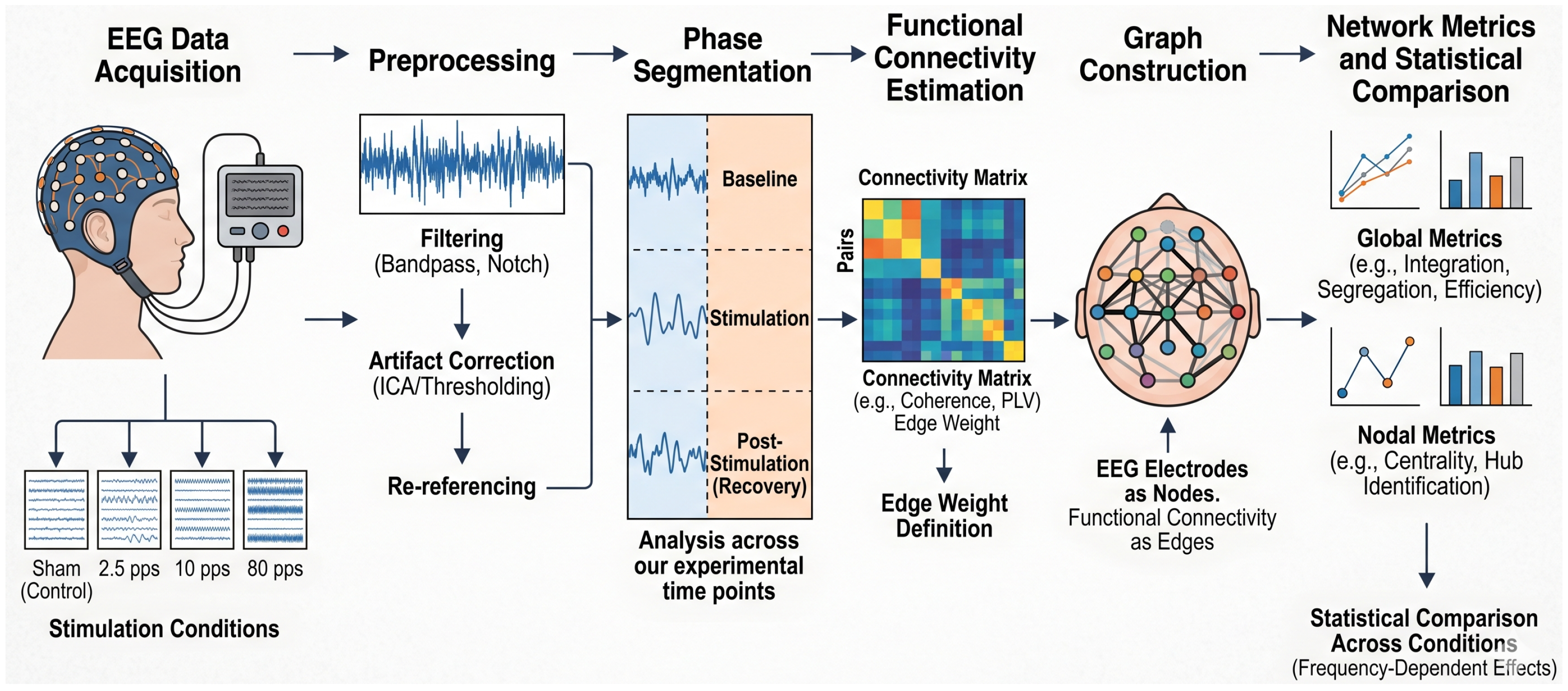
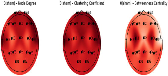
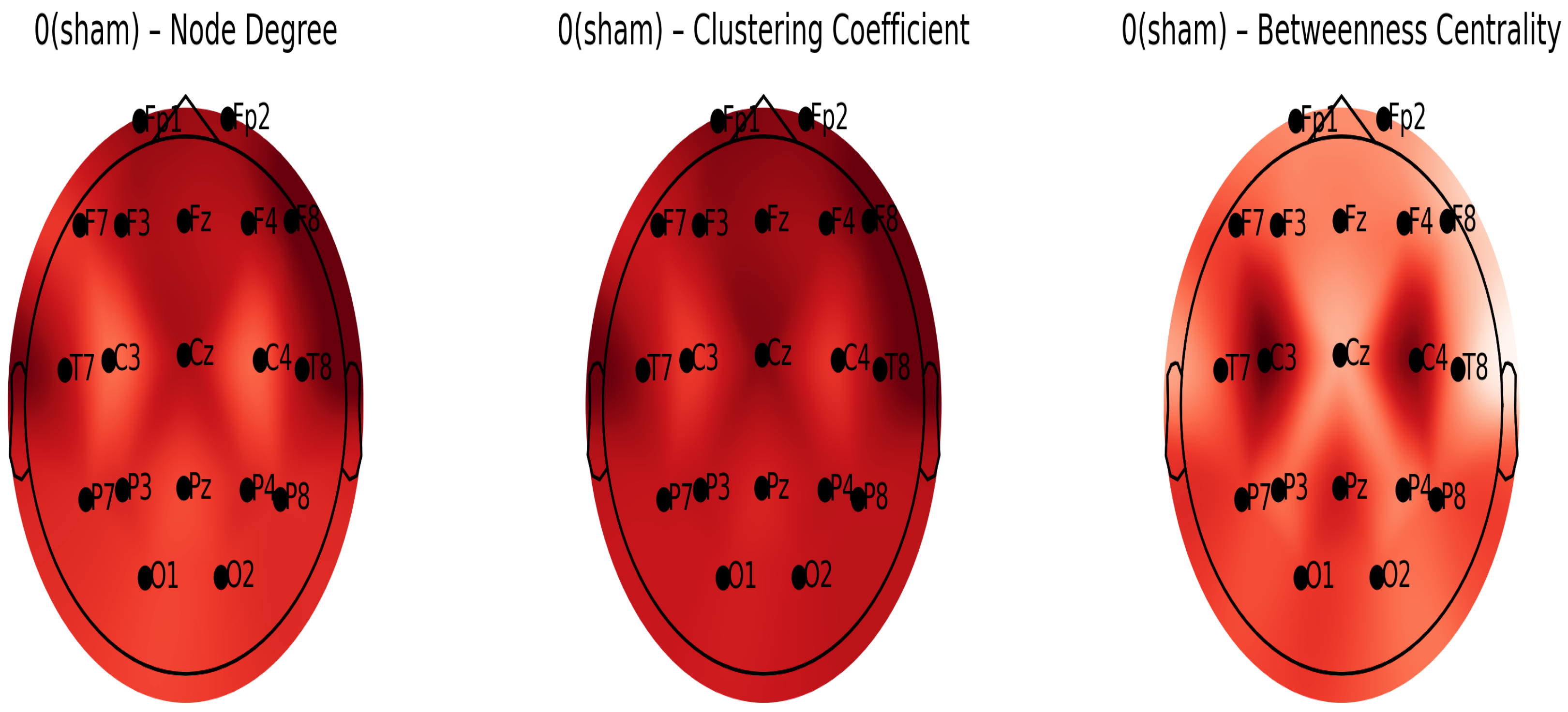
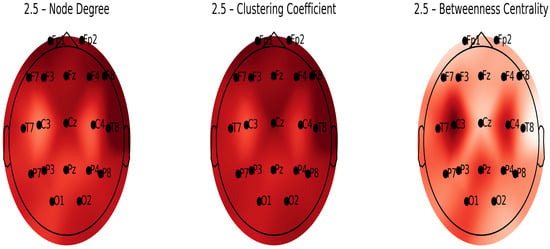
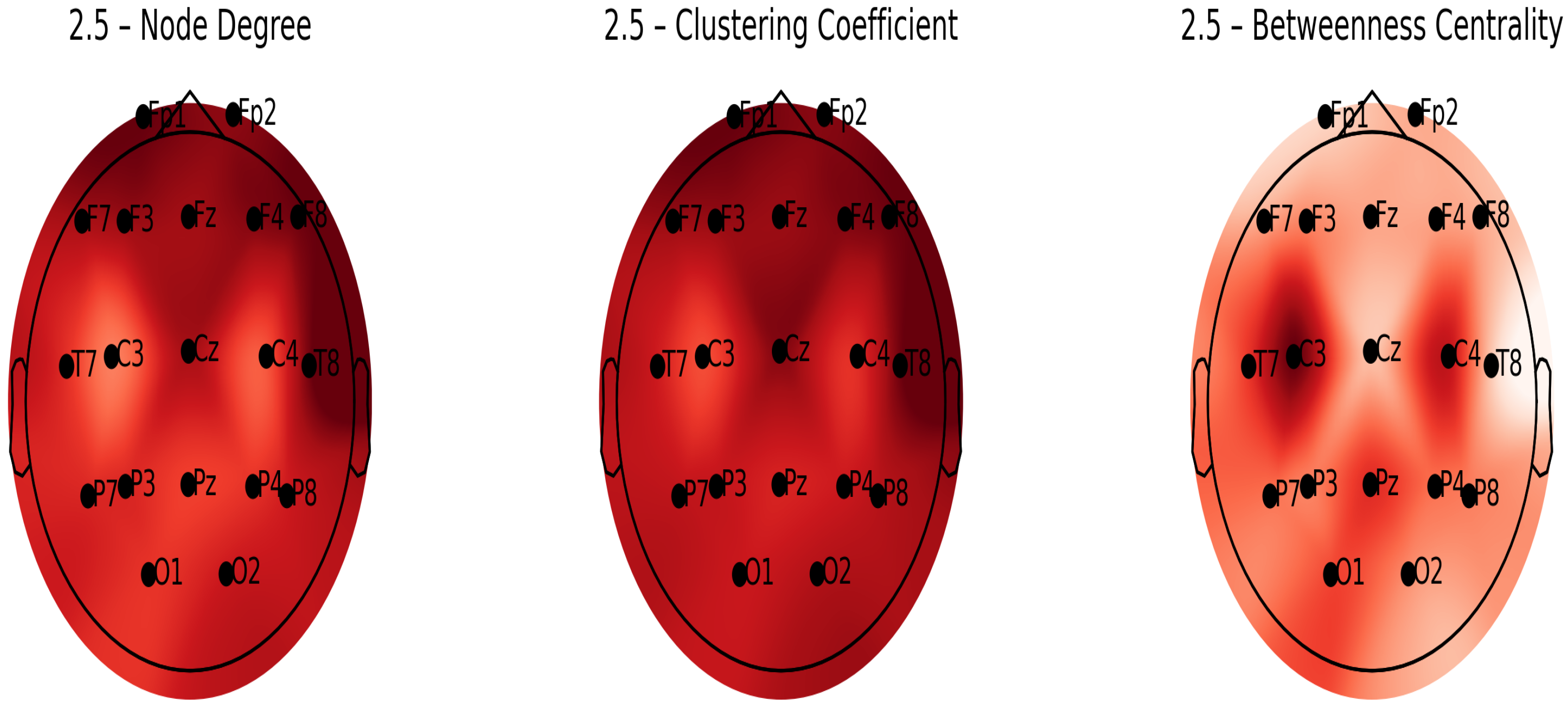
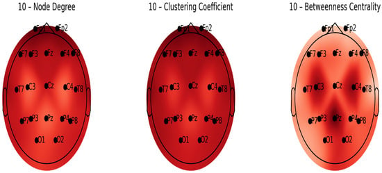
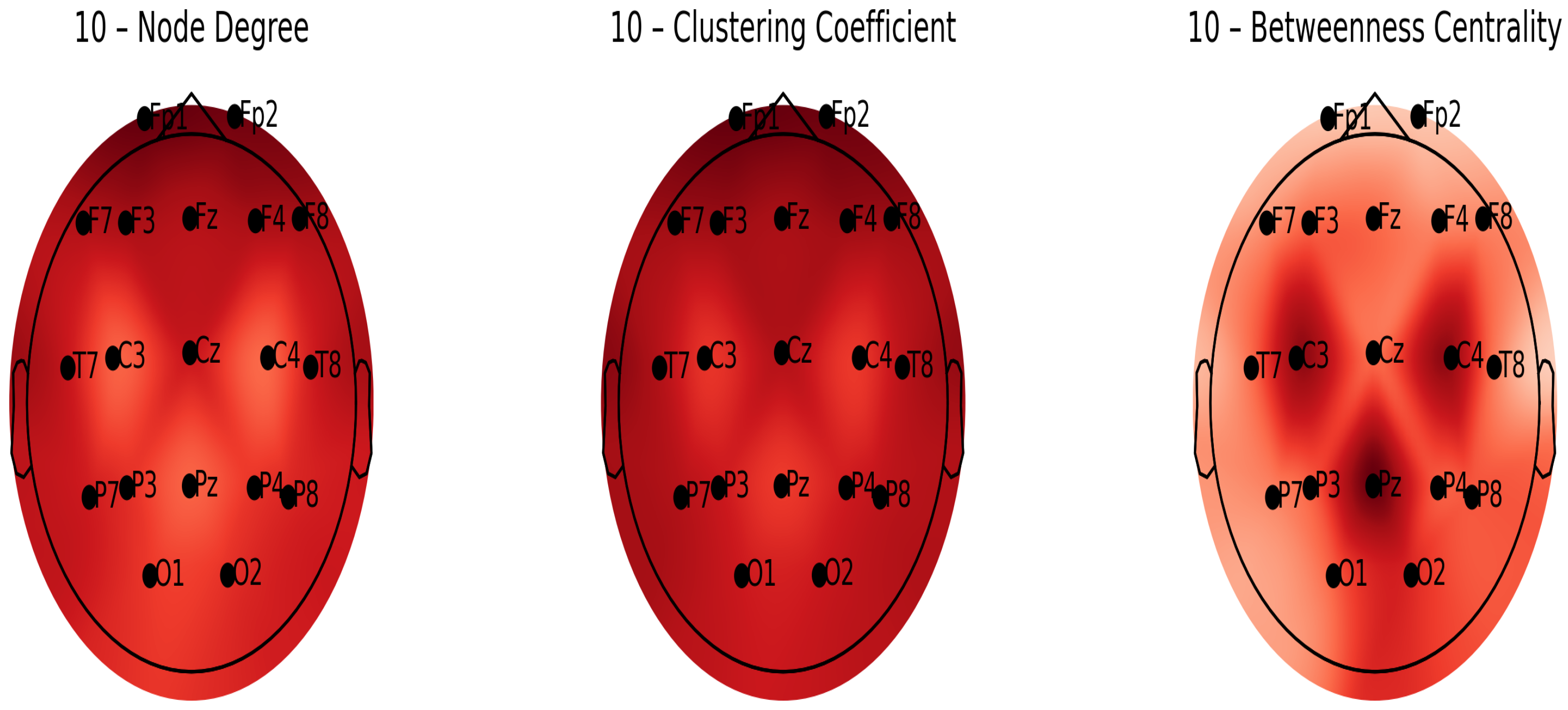
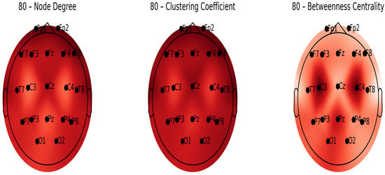
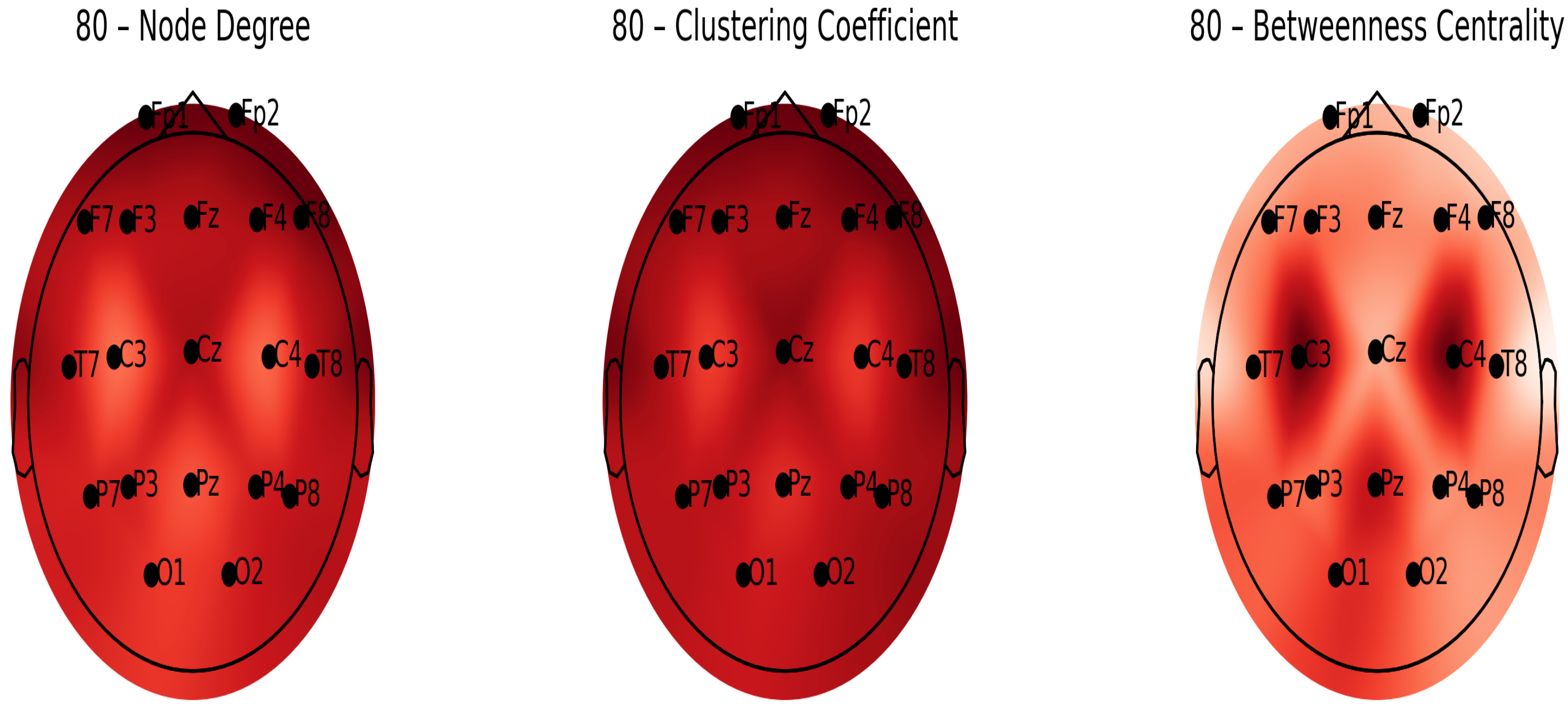
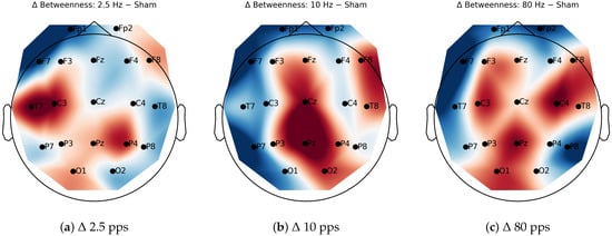
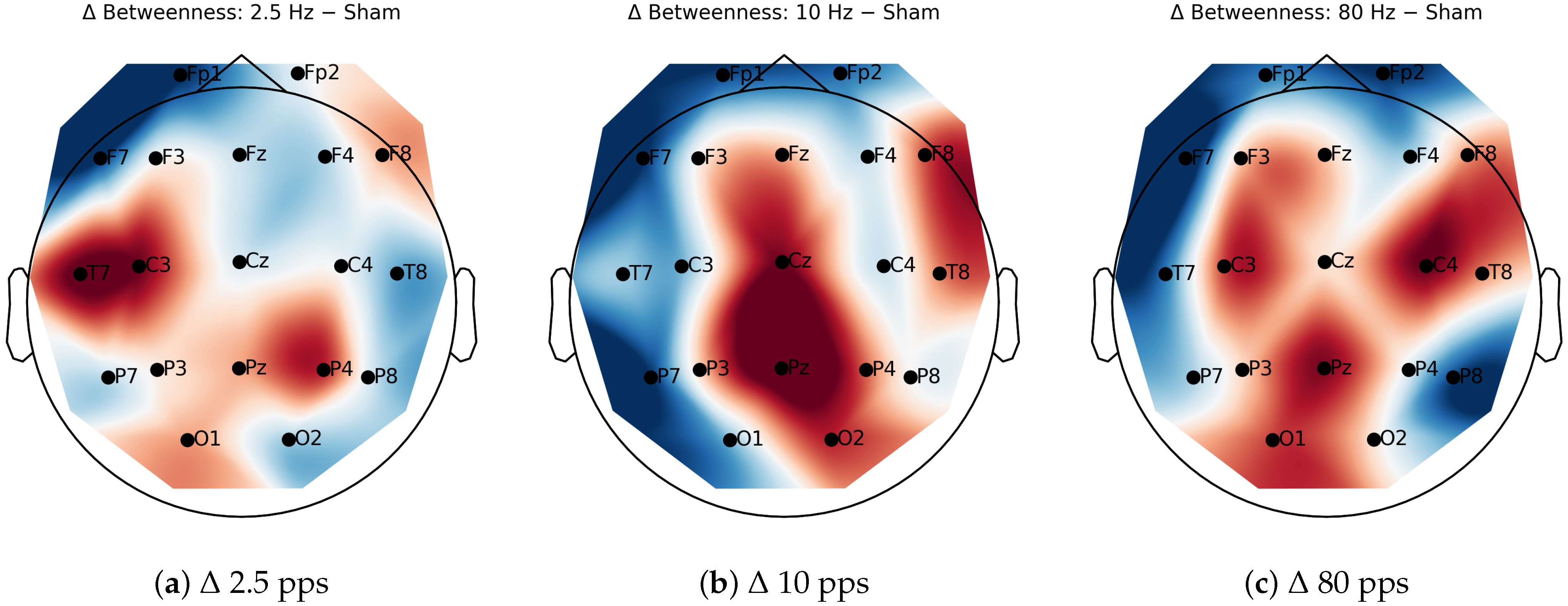
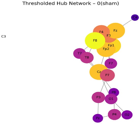
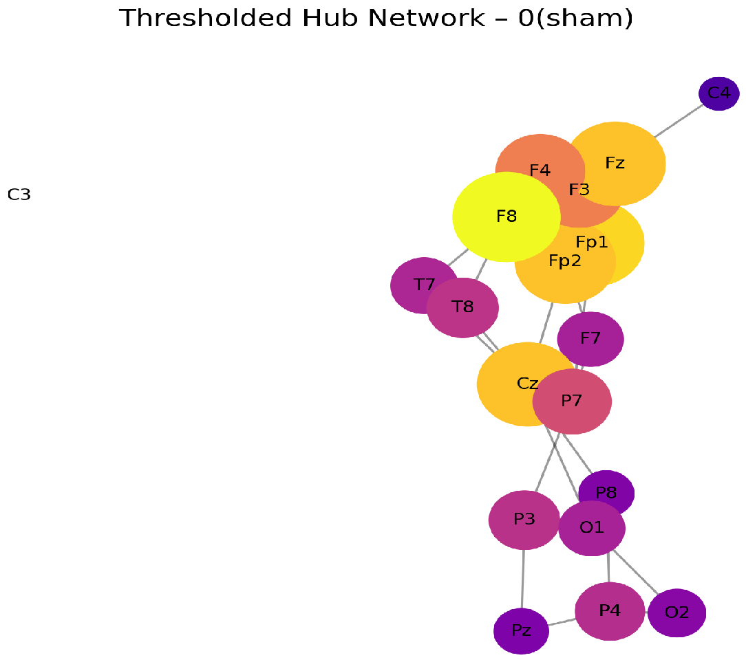
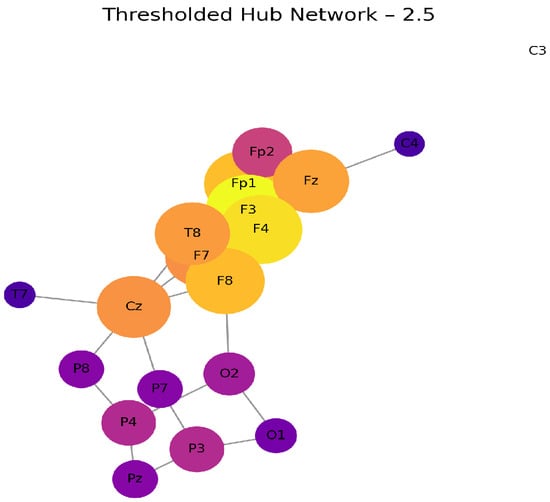
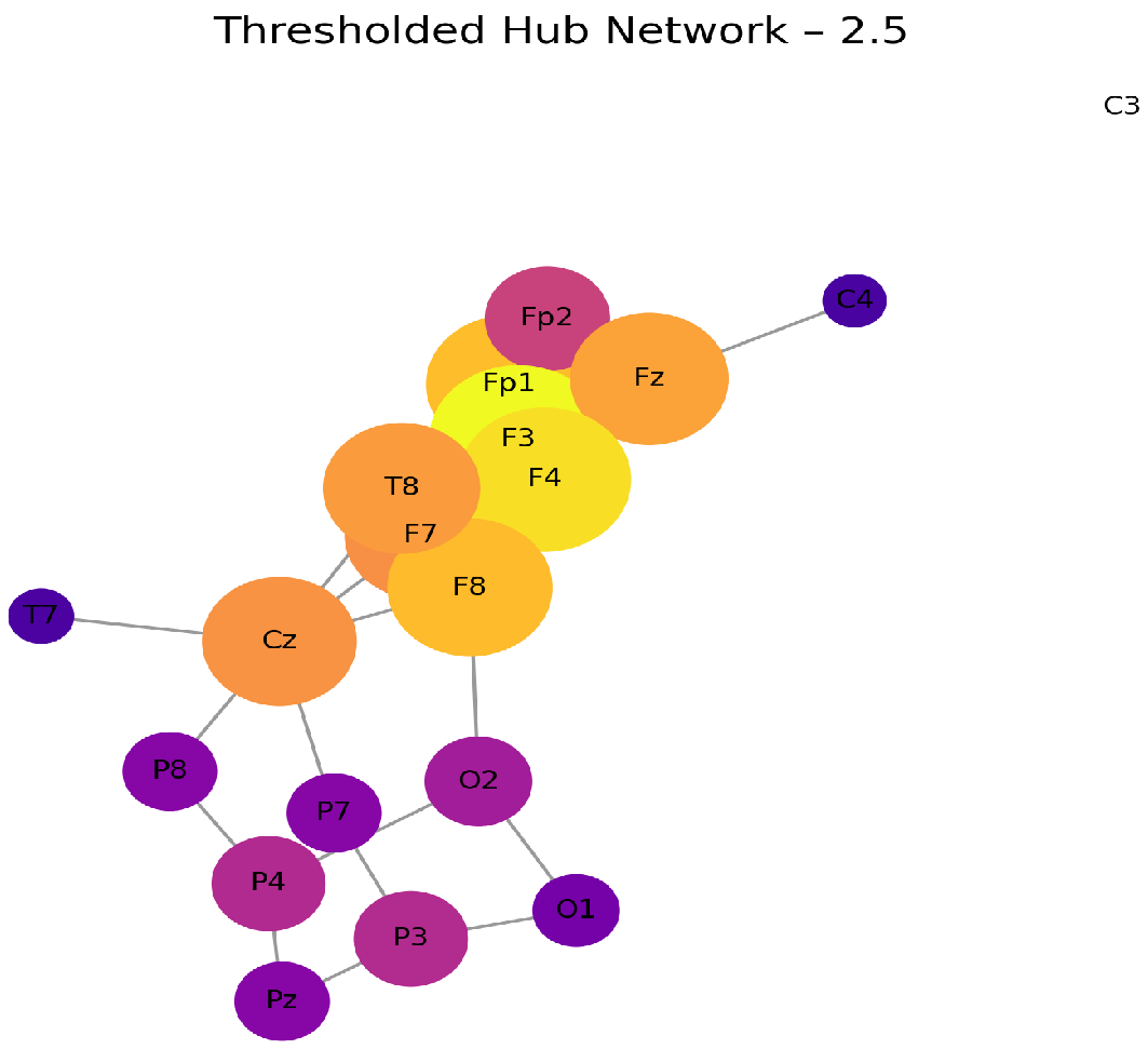
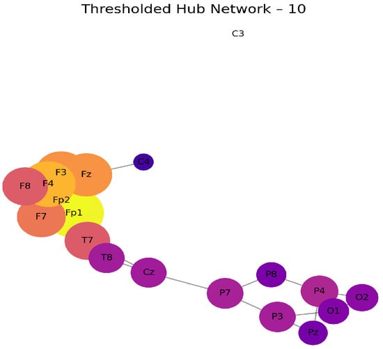
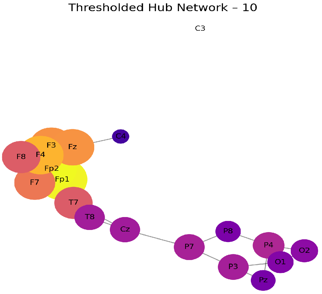
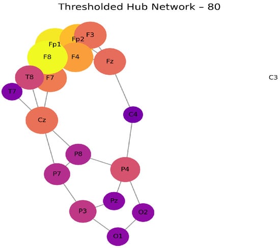
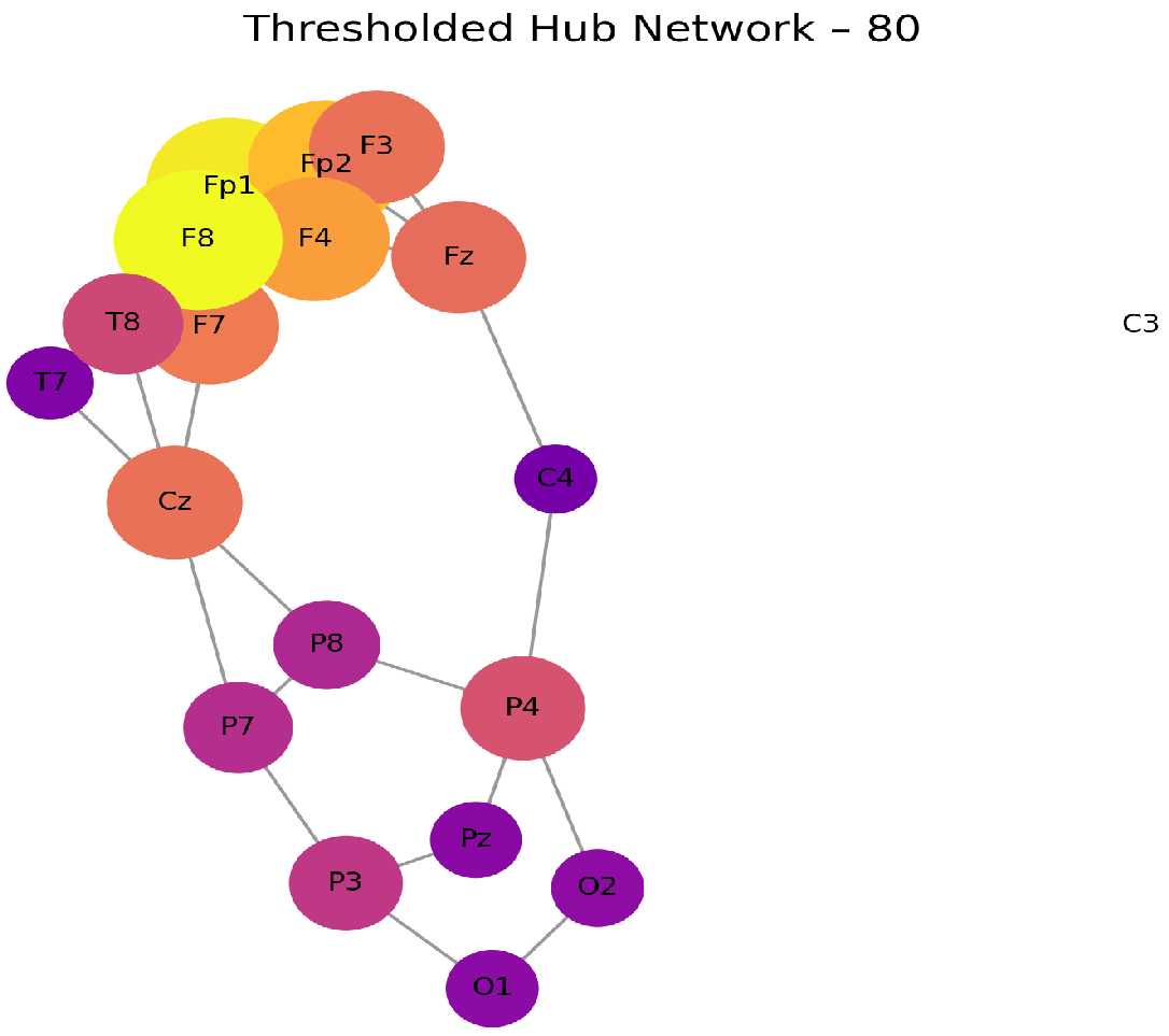

Disclaimer/Publisher’s Note: The statements, opinions and data contained in all publications are solely those of the individual author(s) and contributor(s) and not of MDPI and/or the editor(s). MDPI and/or the editor(s) disclaim responsibility for any injury to people or property resulting from any ideas, methods, instructions or products referred to in the content. |
© 2026 by the authors. Licensee MDPI, Basel, Switzerland. This article is an open access article distributed under the terms and conditions of the Creative Commons Attribution (CC BY) license.