


Abstract
Automated weed classification supports site-specific weed management by enabling targeted interventions and reducing environmental and operational costs. This study presents a multi-seed evaluation of six deep learning configurations—YOLO26n-cls, Vision Transformer (ViT-B/16), DINOv2 (ViT-S/14) with linear probing and full fine-tuning, ResNet-50, and EfficientNet-B0—for nine-class weed classification using a stratified subset of the DeepWeeds benchmark. The models were evaluated using a leakage-checked train/validation/test split and repeated training across multiple random seeds to assess performance stability and statistical reliability. Among the evaluated approaches, DINOv2-FT and EfficientNet-B0 demonstrated the strongest overall performance, while statistical analysis showed that differences among several high-performing models were not consistently significant across seeds. The study also identifies the importance of appropriate transfer-learning strategies and hyperparameter selection, demonstrating that model performance can be strongly affected by optimisation choices. A reproducibility issue affecting ViT-B/16 was identified and transparently reported, leading to its exclusion from multi-seed statistical comparisons. An exploratory out-of-distribution probe using unlabelled Albanian field images further highlights the challenges of geographic domain shift and the need for locally collected, labelled datasets before reliable regional deployment. Overall, this work provides a systematic comparison of modern deep learning architectures for weed classification and emphasises reproducibility, statistical validation, and careful interpretation of model rankings.
1. Introduction
Weed competition reduces crop yields and drives reliance on broad-spectrum herbicides, imposing substantial economic and environmental costs on agriculture. Site-specific weed management (SSWM) addresses this by restricting chemical treatment to confirmed weed-infested areas, but it requires accurate and timely plant classification from mobile-device imagery captured under variable field conditions. Architecture selection is therefore a critical design decision, given the trade-offs between classification accuracy and inference latency. The rapid growth of deep learning has produced a diverse ecosystem of vision models, ranging from lightweight convolutional neural networks optimised for edge inference to large-scale Vision Transformers pre-trained on hundreds of millions of images. Although general-purpose benchmarks have demonstrated the broad capabilities of these architectures, their comparative behaviour under domain-specific, data-scarce agricultural conditions remains insufficiently characterised. A further complication arises from geographic domain shift: weed species composition, soil texture, illumination, and canopy cover vary substantially across regions, so a model that performs well on a benchmark dataset may degrade on in-field data from a different continent. This study addresses these issues through a controlled comparative experiment involving six configurations—YOLO26n-cls (the nano-scale image classification variant of the Ultralytics YOLO26 family, implemented via the Ultralytics framework), ViT-B/16, DINOv2 under both linear probing (DINOv2-LP) and full fine-tuning (DINOv2-FT), ResNet-50, and EfficientNet-B0—trained on a stratified subset of the DeepWeeds benchmark, with five of the six configurations independently trained across three random seeds (Section 4.1.2 discloses why ViT-B/16 could not be). In addition to standardised benchmark evaluation, we conduct an exploratory, unlabelled out-of-distribution (OOD) probe in which the trained models are applied to 350 mobile-captured images from Albanian agricultural and urban environments. We deliberately use the term “OOD probe” rather than “cross-domain evaluation” throughout this paper, because the absence of ground-truth labels means no accuracy, error rate, or misclassification analysis could be performed on the Albanian images; the experiment characterises prediction behaviour, not classification performance, under geographic domain shift. The proliferation of pre-trained models via platforms such as PyTorch Hub and Hugging Face has lowered the barrier to applying state-of-the-art architectures to domain-specific problems. However, accessibility does not imply applicability: transfer-learning strategies—full fine-tuning, linear probing, and frozen feature extraction—exhibit markedly different behaviours on small datasets, and the choice of strategy may matter as much as the choice of architecture. This distinction is particularly consequential in precision agriculture, where labelled training data are costly to acquire and annotate. The creation of high-quality labelled image datasets remains a major bottleneck in computer vision because manual annotation is costly, time-consuming, and susceptible to inconsistencies. Human-in-the-loop annotation frameworks can reduce this burden by combining AI-assisted predictions with expert verification and iterative label refinement [1]. DINOv2 is evaluated under both linear probing and full fine-tuning, allowing the effect of transfer strategy to be examined while holding the backbone identity fixed. Nevertheless, the broader architecture comparison remains partly confounded by framework-specific training procedures and model-specific optimisation settings. Consequently, performance differences should not be attributed exclusively to backbone architecture; this limitation is discussed further in Section 4.1 and Section 6. Beyond predictive accuracy, deployment on agricultural robotic platforms imposes strict constraints on inference latency and memory footprint. A model that offers marginally higher accuracy but requires substantially greater inference time may be impractical for real-time spraying systems that must make actuation decisions at frame rate. Jointly evaluating accuracy and efficiency is therefore essential for translating research outcomes into deployable field systems, although, as discussed in Section 5.6, our own latency comparison is only partially suited to this purpose because measurements were not collected under a common inference framework. Together, these considerations motivate a rigorous empirical study that assesses architectural performance under data scarcity, examines the effect of transfer-learning strategy on per-class performance, quantifies inference latency under a shared hardware budget, and characterises out-of-distribution prediction behaviour across a geographic domain boundary.
1.1. Problem Context
Weed classification in naturalistic pastoral environments is a challenging recognition problem. Models must handle substantial intra-class appearance variation caused by differences in illumination, developmental stage, and occlusion, while simultaneously preserving inter-class discriminability between morphologically similar species with overlapping spectral signatures. The scarcity of labelled agricultural imagery compounds these difficulties, making transfer learning and self-supervised pre-training the primary routes to practical accuracy. Analogous challenges—domain-specific classification under limited labelled data—arise in other applied deep learning contexts, such as building attribute classification from street-view imagery for seismic risk assessment [2], where transfer learning similarly provided the essential performance foundation.
1.2. Contributions
This paper makes the following contributions:
- A multi-seed evaluation pipeline comparing six convolutional and Transformer configurations under a controlled data and compute budget, with five of the six independently trained across three random seeds on a leakage-checked, per-class-stratified split, and all training and evaluation code intended for public release (Data Availability Statement).
- An empirical comparison of full fine-tuning versus linear probing transfer strategies on a domain-specific nine-class weed benchmark (DINOv2-LP vs. DINOv2-FT), directly isolating the effect of the transfer strategy from the backbone identity.
- A statistically grounded, multi-seed performance analysis, including pairwise McNemar significance tests with Holm–Bonferroni correction for all ten pairwise comparisons among the five validly trained models.
- A learning-rate sensitivity analysis for EfficientNet-B0, showing that its previously observed underperformance was a hyperparameter artefact rather than an architectural limitation.
- A transparent root-cause diagnosis of a software-library incompatibility that silently corrupted a ViT-B/16 training run, offered as a methodological case study in detecting and honestly reporting reproducibility failures rather than a further architectural finding.
- A per-class failure analysis identifying systematic failure modes not captured by aggregate accuracy metrics, with confidence intervals reported for claims resting on small class supports.
- An exploratory out-of-distribution probe on 350 mobile-captured Albanian field and urban images, explicitly reported as a hypothesis-generating exercise requiring future validation with labelled data, not as a cross-domain accuracy evaluation.
2. Related Work
This section situates the present study within prior research on agricultural image classification, Transformer-based vision models, self-supervised representation learning, and transfer-learning methodology, with emphasis on the strands most directly relevant to weed classification, transfer learning under data scarcity, and domain shift.
2.1. Convolutional Approaches in Agricultural Vision
Olsen et al. [3] created the DeepWeeds dataset and set ResNet and Inception baselines for classifying different types of weeds in Australian pastoral settings. More recent work has extended deep learning for agricultural vision to UAV-based weed and crop segmentation [4] and knowledge-based weed segmentation pipelines [5]. The translation equivariance and local receptive field structure of convolutional networks correspond effectively with the spatially localised texture features that are inherently crucial in botanical imagery. Recent reviews also indicate that deep learning frameworks, particularly advanced YOLO architectures, consistently outperform traditional machine-vision approaches in challenging field conditions characterised by variable illumination and occlusion [6]. Further work has investigated lightweight CNN–Transformer hybrids such as YOLO-SW, which improve both real-time inference speed and detection accuracy for embedded agricultural machinery [7].
2.2. Vision Transformers
Dosovitskiy et al. [8] redefined image recognition as sequence modelling applied to fixed-size image patches. ViT models excel at long-range spatial reasoning, but they require large-scale pre-training to match the efficiency of convolutional architectures in low-data regimes. Recent research has focused on the application of ViTs to agricultural datasets, demonstrating that self-attention mechanisms substantially enhance the modelling of complex global relationships in botanical imagery relative to conventional localised CNNs [9]. A pure patch-based Transformer trained directly on UAV-acquired crop and weed imagery, with no convolutional layers at all, achieved classification accuracy competitive with CNN baselines, further supporting the viability of attention-only architectures for agricultural remote sensing [10]. Variants such as the Swin Transformer have demonstrated exceptional efficacy in fine-grained weed recognition by computing self-attention within dynamic windows, facilitating the differentiation of subtle morphological variations between weeds and crops [11].
2.3. Self-Supervised Representation Learning
Aided by a self-distillation objective with no manual supervision, DINOv2 [12] trains large Vision Transformers that generate representations with strong linear separability properties. Linear probing—a method of embedding a single linear layer onto a frozen backbone—offers a direct measure of the semantic quality of a pre-trained feature space, without domain-specific gradient adaptation. To improve generalisability across diverse agricultural sectors, modern methods such as WeedNet have employed self-supervised learning to develop foundation models for global weed species [13]. Recent methods have also employed contrastive learning frameworks, including WeedCLR and SimSiam, to address the long-tailed class imbalances present in real-world agricultural datasets [14].
2.4. YOLO-Based Weed Detection Systems
The You Only Look Once (YOLO) family of object detectors has become a cornerstone of weed detection research owing to its single-stage architecture, which performs classification and localisation in a single forward pass. One of the most comprehensive benchmarking studies in this area was conducted by Dang et al. [15], who assembled the CottonWeedDet12 dataset, comprising 5648 images across 12 weed classes with 9370 bounding box annotations, and evaluated 25 YOLO variants spanning seven versions (YOLOv3 through YOLOv7), reporting mAP@0.5 scores ranging from 88.14% (YOLOv3-tiny) to 95.22% (YOLOv4), with Scaled-YOLOv4 achieving the best mAP@[0.5:0.95] of 89.72%. Kumar et al. [16] assessed YOLOv8-nano on a 1300-image agricultural dataset, reporting an overall accuracy of approximately 86% and per-class IoU values of 0.765 (crops) and 0.763 (weeds), while noting persistent weed–background confusion. Upadhyay et al. [17] developed optimised YOLO-based models for multi-class weed and crop detection on edge devices using 4828 annotated field images; lightweight variants such as YOLO11n achieved an mAP of 0.83 with fast inference. Jin et al. [18] proposed a crop-detection-first strategy for weed identification in vegetable fields, in which non-crop regions are treated as weeds; YOLOv3 achieved the best performance (F1 = 0.971) among the detectors compared, with better computational efficiency than Faster R-CNN. These studies collectively motivate the use of lightweight YOLO variants under real-time constraints and provide a performance reference for the present study’s benchmarking methodology, while also illustrating that YOLO-family models in the agricultural literature are used overwhelmingly in detection mode with bounding-box output—a capability that the classification-only YOLO26n-cls variant used here does not provide (see Section 5.6). A recent comparison of YOLO26-nano against Transformer-based detectors (RT-DETR, RF-DETR) for early weed detection in tomato plantations reported the same efficiency-versus-context trade-off observed in the present benchmark: CNN-based detectors achieved strong performance at lower computational cost, while Transformer-based approaches captured broader spatial context with a higher resource demand [19].
2.5. Transfer-Learning Strategies for Agricultural Vision
Transfer learning has become the dominant paradigm for deploying deep learning models in data-scarce agricultural settings, where acquiring and annotating large labelled datasets is costly and time-consuming. Three principal strategies are commonly employed: (i) full fine-tuning, in which all backbone parameters are updated during training on the target domain; (ii) linear probing, in which the backbone is frozen and only a single classification head is trained; and (iii) frozen feature extraction with data augmentation, which relies entirely on pre-trained representations without any gradient updates to the backbone. For large-parameter models such as ViT-B/16, full fine-tuning on small datasets risks catastrophic forgetting of generic visual features and overfitting to training-set idiosyncrasies, whereas linear probing preserves pre-trained representations at the cost of reduced domain adaptation [8]. A lightweight CNN–Transformer hybrid combining contrastive learning with pseudo-labelling has recently been proposed for few-shot recognition of rare, toxic weed species, achieving 80.3% accuracy in the few-shot setting while sustaining 18.9 FPS on a Jetson Nano at under 5.1 W [20].
In the present study, we compare full fine-tuning (ViT-B/16, ResNet-50, EfficientNet-B0, YOLO26n-cls) against linear probing (DINOv2) under a controlled data budget; we emphasise that this design confounds transfer strategy with model identity for DINOv2 specifically, and any claims about DINOv2’s representation quality in isolation from its transfer strategy should be read with this confound in mind. A promising direction for future work is to additionally evaluate parameter-efficient fine-tuning methods such as LoRA, which would occupy a middle ground between full fine-tuning and linear probing and were outside the scope of the present comparison. Espejo-Garcia et al. [21] directly compared linear probing, full fine-tuning, and parameter-efficient LoRA fine-tuning of DINOv2 across disease detection, weed identification, and growth-stage classification tasks, finding that DINOv2 generalised well across datasets at a markedly lower training cost than full fine-tuning. Transfer learning has been successfully applied to specialised image classification tasks, where pre-trained convolutional and Transformer-based backbones reduce dependence on large task-specific datasets, accelerate convergence, and support better generalisation across diverse visual domains [2,22].
2.6. Research Gaps Addressed by the Present Study
The preceding review reveals several gaps that the present study is designed to address. First, while YOLO detectors have been extensively benchmarked on North American and Western European weed datasets, no published study has evaluated these models on Albanian agricultural and urban field images, where weed species composition, soil characteristics, and imaging conditions differ substantially from previously studied environments; the present study offers an initial, exploratory characterisation of this setting rather than a validated benchmark. Second, most existing comparative studies focus exclusively on CNN-based detectors; the potential of Vision Transformer architectures and self-supervised feature extractors such as DINOv2 for weed classification has not been systematically benchmarked alongside YOLO-family classification models under identical data and compute constraints. Third, cross-domain out-of-distribution prediction behaviour—how a model trained on one crop–weed system responds when applied to an unseen geographic domain—has been identified as a critical open question [3,5] but has rarely been probed empirically, even in an unlabelled, exploratory form. A hierarchical DINOv2-based segmentation framework trained on multi-year European weed data maintained meaningful performance when transferred to unseen sensors, seasons, and a new continent, with species-level F1 dropping from 0.87 in-distribution to 0.77 under moderate shift and 0.44 under extreme sensor shift, compared to 0.24 and 0.14 for prior CNN baselines [23] These domain-shift challenges are not unique to weed recognition: a broader review of domain adaptation across agricultural image-analysis tasks—including crop health monitoring, pest detection, and fruit identification—confirms that environmental variation, sensor differences, and cross-region acquisition are pervasive obstacles to model generalisation throughout precision agriculture [24].
Several prior studies have proposed techniques for closing this domain gap directly: unsupervised domain adaptation for crop–weed recognition across diverse, previously unseen farmlands [25], domain-adaptive semantic segmentation for agricultural robots operating across different crops, sensors, and seasons [26], and a comparison of Fourier-transform-based and CycleGAN-based adaptation for weed segmentation across differing robot platforms and acquisition years [27]. These approaches typically require access to unlabelled target-domain images during training in order to adapt; in contrast, the present study evaluates models with zero exposure to the target domain at any stage, characterising raw out-of-distribution prediction behaviour rather than attempting to close the domain gap through adaptation.
Fourth, the comparative effect of different transfer-learning strategies (full fine-tuning vs. linear probing) on per-class performance under severe data scarcity is underexplored. The present study addresses these gaps through a controlled comparative evaluation of YOLO26n-cls, Vision Transformers, DINOv2, and classical CNN baselines, together with an exploratory, unlabelled OOD prediction probe on a novel Albanian image collection.
3. Dataset Description
The DeepWeeds dataset [3] contains high-resolution images of eight invasive weed species that are native to Australian pastoral land, as well as a negative background class. The nine classes are: Chinee apple, Lantana, Parkinsonia, Parthenium, Prickly acacia, Rubber vine, Siam weed, Snake weed, and Negative. Figure 1 shows a sample of independent test-set images with their ground-truth class labels.
Figure 1.
A random batch of 16 images from the independent test set with their ground-truth class labels, illustrating the visual difficulty of the task: several classes (e.g., Parthenium, Parkinsonia) are visually similar to Negative background vegetation at this image scale.
3.1. Data Partitioning
The dataset used throughout this study is a properly per-class-stratified subsample with a genuine three-way split. We drew a fixed 20% subsample (data-split seed 42, via scikit-learn’s train_test_split with stratify= set to the class label) of the full 17,509-image DeepWeeds corpus, yielding 3501 images, partitioned 70/15/15 into a training set of 2450 images, a validation set of 525 images (used for model selection and early stopping), and a held-out independent test set of 526 images that was never used for any training or hyperparameter decision and on which all headline metrics in Section 5 were recorded. This procedure stratifies independently within each of the nine classes, so per-class train/val/test proportions track the target 70/15/15 split to within 0.3 percentage points for every class (Table 1); we additionally verified programmatically that no filename appears in more than one split, confirming zero train/validation/test leakage. The Negative class constitutes approximately 52% of every split, reflecting the natural class imbalance of the full dataset. Table 1 reports the resulting per-class distribution. The five validly re-trained configurations share this fixed stratified train/validation/test manifest. The provisional ViT-B/16 result originates from an earlier, non-comparable split and is reported separately. Five of the six model configurations—ResNet-50, EfficientNet-B0, DINOv2-LP, DINOv2-FT, and YOLO26n-cls—were independently trained or fine-tuned under their specified transfer-learning protocols across three random seeds (42, 123, and 2026). The seeds controlled the initialisation of newly added trainable layers, stochastic data augmentation, and DataLoader shuffling, while the data split was held fixed across runs. Each trained model was evaluated once per seed on the same independent test set, and the mean and standard deviation across the three runs are reported for all headline metrics. The sixth configuration, ViT-B/16, could not be validly trained under this protocol due to a software-environment issue described in Section 4.1.2; its single-seed result is retained and excluded from the multi-seed and significance analyses, flagging this explicitly wherever it arises. Wherever a per-class claim rests on fewer than 25 test images, we continue to report a 95% Wilson score confidence interval alongside the point estimate.
Table 1.
Per-class image counts in the training, validation, and independent test splits used throughout this study (20% stratified subsample of DeepWeeds, data-split seed 42). Every class’s split proportions track the target 70/15/15 ratio to within 0.3 percentage points; zero filename overlap across splits was confirmed programmatically.
3.2. Albanian Field Dataset
To probe cross-domain out-of-distribution prediction behaviour, we collected a secondary, unlabelled dataset of 350 images captured in Albanian urban and rural environments in Tirana city and the surrounding rural areas of the Tirana region, during spring 2026, using a consumer smartphone camera (Samsung Galaxy A52s 5G; native resolution pixels, downsampled to for inference). The images cover local plant and weed species not present in the DeepWeeds benchmark, photographed under natural outdoor lighting conditions at varying distances (approximately 0.3–2.0 m) and orientations. Subjects include plants growing in pavement cracks, along stone and brick walls, in gravel and soil patches, and in open agricultural field settings. We use the term “field dataset” loosely here to mean mobile-acquired, real-world Albanian imagery; we acknowledge that a meaningful fraction of the images depict urban and peri-urban vegetation (pavement cracks, walls) rather than cultivated agricultural fields, and we do not describe this collection as representative of Albanian agricultural conditions specifically—it is better characterised as a convenience sample of local flora useful for probing OOD behaviour, not a systematically sampled agricultural survey. A systematic, season- and crop-stratified collection remains future work. Recent dataset research has demonstrated that high-quality annotations, sufficient dataset scale, and geographic diversity are important for developing models that remain robust across heterogeneous environments. Geographically restricted or inconsistently annotated datasets may consequently limit model generalisation beyond their original acquisition conditions. The dataset presents several inherent challenges. First, a small-target recognition problem arises when plants occupy a small fraction of the image frame, particularly in pavement-crack contexts where subjects may cover fewer than 5% of the image pixels. Second, a fine-grained recognition challenge is present because many local weed species share similar leaf morphology and colour with the Australian species in the training set. Third, significant background clutter is introduced by urban surfaces (concrete, brick, gravel) that differ markedly from the pastoral backgrounds in DeepWeeds. No ground-truth taxonomic labels exist for this dataset, as the nine Australian invasive species in the training set do not occur in Albanian fields; assigning those labels would be taxonomically meaningless. Because of this, the dataset cannot support a classification accuracy evaluation of any kind: it serves exclusively as an unlabelled probe of prediction behaviour under geographic domain shift, and every result derived from it in this paper is reported as an exploratory, hypothesis-generating observation rather than a performance metric. To facilitate reproducibility and future research, the Albanian Field Images dataset will be made publicly available upon paper acceptance, and we additionally plan to release a manually annotated (at minimum, plant-vs-background) subset in a future study so that a genuine accuracy evaluation becomes possible. Figure 2 shows nine representative samples from the collection.
Figure 2.
Nine representative samples from the Albanian field dataset collected via mobile device. Images show diverse plant species growing in urban and semi-rural environments in Albania, including plants in pavement cracks, against stone and brick walls, in gravel patches, and in open field settings. No ground-truth class labels are available for this dataset.
4. Methodology
Figure 3 summarises the complete experimental pipeline, from data input through to the exploratory out-of-distribution probe. All experiments were run in Python 3.12.13 with PyTorch 2.11.0+cu128, torchvision 0.26.0, Ultralytics 8.4.102, Hugging Face transformers 5.14.1, scikit-learn 1.5.2, NumPy 2.1.3, SciPy 1.14.1 and Matplotlib 3.9.2, on a single NVIDIA Tesla T4 GPU (NVIDIA Corporation, Santa Clara, CA, USA). Grad-CAM visualisations used pytorch-grad-cam 1.5.4.
Figure 3.
Overview of the experimental methodology pipeline, from data input through preprocessing and augmentation, parallel multi-seed training of six configurations, unified evaluation, and the exploratory out-of-distribution prediction probe on Albanian field images. The asterisk (*) marks ViT-B/16, the single configuration that could not be validly trained under the multi-seed protocol and is therefore excluded from all multi-seed, McNemar and out-of-distribution comparisons (Section 4.1.2). The figure was created using an AI-assisted visualisation tool and subsequently edited and verified by the authors to ensure scientific accuracy.
Training images were augmented using random resized cropping (scale , output resolution ), random horizontal and vertical flipping ( each), random rotation (), and colour jitter (brightness, contrast, and saturation ). Validation images were resized to pixels without stochastic augmentation. All images were normalised using ImageNet population statistics (, ). No class-balancing mechanism (weighted loss, focal loss, or resampling) was applied during training; the Negative class was left at its natural 52% frequency in both splits. This was a deliberate choice to reflect the class distribution a practitioner would encounter with no additional intervention, but we acknowledge in Section 4.1 that it likely disadvantages minority classes such as Snake weed, Rubber vine, and Lantana, and that class-balancing strategies are a natural next step.
4.1. Experimental Design
All models were evaluated on the same training/validation/test split (Section 3.1), input resolution, augmentation pipeline, loss function (cross-entropy), and evaluation metrics. The training protocol was not identical across models, which remains a confound for any claim of architectural superiority. YOLO26n-cls was trained through the Ultralytics classification pipeline, which applies its own automatic cosine learning-rate schedule, Automatic Mixed Precision, and internal training recipe (maximum 30 epochs, patience 5, batch size 16); the four PyTorch models (ResNet-50, EfficientNet-B0, DINOv2-LP, DINOv2-FT) were trained with a manually specified AdamW recipe (cosine annealing, maximum 30 epochs, patience 5, batch size 16, mixed precision) at per-model learning rates individually justified below rather than a single uniform rate (Section 4.1.4). These differences mean that part of YOLO26n-cls’s accuracy and latency may still be attributable to its highly-optimised, framework-specific training and inference pipeline rather than to its architecture per se; we report this as a limitation of the present comparison rather than attempt to retrofit a false appearance of uniformity. Transfer learning from large-scale pre-trained weights has demonstrated consistent benefits across diverse visual recognition tasks [8,12], and is well suited to the data-constrained botanical domain studied here.
4.1.1. YOLO26n-cls Classification
In this study, we used the YOLO26n-cls model, the nano-scale image classification variant of the Ultralytics YOLO26 family, implemented through the Ultralytics framework [28] (Ultralytics 8.4.102, Python 3.12.13, PyTorch 2.11.0+cu128, trained on a single NVIDIA Tesla T4 GPU with Automatic Mixed Precision, data-split seed 42; confirmed directly from the executed training notebook’s logged environment record). We note explicitly that the YOLO26n-cls backbone was pre-trained on ImageNet-1K only, like ResNet-50 and EfficientNet-B0; it was not pre-trained at the larger scale of ViT-B/16 (ImageNet-21K) or DINOv2 (self-distillation on hundreds of millions of images). YOLO26n-cls is a lightweight convolutional architecture that employs C2PSA and C3k2 convolutional blocks, comprising approximately 1.54 million parameters and requiring 3.3 GFLOPs per forward pass. Although the YOLO family is widely known for object detection, the -cls classification variant removes the detection head and replaces it with a global average pooling layer followed by a linear classifier, making it directly comparable to the pure classification models in this benchmark but, correspondingly, unable to output bounding boxes (see Section 5.6). For each of the three training seeds (42, 123, 2026), the model was trained for up to 30 epochs with early stopping (patience of 5 epochs on validation top-1 accuracy; training converged and stopped between epochs 16 and 20 across the three seeds), a batch size of 16, an input resolution of , AdamW optimisation with automatic cosine learning-rate scheduling, and Automatic Mixed Precision (AMP). Per-seed training logs (final top-1 ≈ 0.90, top-5 ≈ 0.99–1.00) show smooth, monotonic convergence with no divergence in any seed. Training data were organised in a class-hierarchical directory structure as required by the Ultralytics classification pipeline.
4.1.2. Vision Transformer Fine-Tuning and a Disclosed Training Failure
ViT-B/16 [8] was initialised with ImageNet-21K pre-trained weights (google/vit-base-patch16-224-in21k). The original classification head was replaced with a randomly initialised linear projection mapping to nine output classes, and all backbone parameters were updated during training (full fine-tuning). Optimisation used AdamW (lr = , weight decay = ) with cross-entropy loss. Disclosure: The multi-seed ViT-B/16 training run described above was invalid and is not reported.While training all six configurations under the stratified multi-seed protocol, the transformers library was upgraded to version 5.14.1. This version introduced a backbone parameter-naming refactor (e.g., encoder.layer.{0..11}.attention.attention.query.weight in the checkpoint versus vit.layers.{0..11}.attention.q_proj.weight expected by the new model class) that is not resolved automatically for this checkpoint: the library’s own weight-loading report showed every backbone and pooler parameter in the pre-trained checkpoint listed as UNEXPECTED (i.e., unused) and every parameter actually instantiated in the model—all twelve Transformer layers, the embeddings, and the classifier—listed as MISSING (i.e., randomly initialised). In effect, the “fine-tuned” ViT-B/16 in this training attempt was trained entirely from random initialisation rather than from ImageNet-21K weights, which is fully consistent with the affected run’s plateauing test accuracy (≈64%, far below a randomly-initialised ViT’s expected ceiling on 2450 training images) and with a softmax-based out-of-distribution-detection AUROC on the Albanian probe images of 0.40–0.46—below the 0.50 level expected of an uninformative detector, and far below the 0.66–0.79 range achieved by every other model (Section 5.9). A ViT-B/16 run with a pinned, pre-refactor transformers version was not available before the evaluation cut-off. To avoid reporting either a known-invalid number or an under-verified new one, a single-seed ViT-B/16 result (86.00% accuracy; per-class metrics are reported in Section 5.2.2) is reported throughout this study, and ViT-B/16 is excluded from every multi-seed, McNemar, and Albanian OOD-detection result reported below, with its absence footnoted wherever the other five models are compared. A ViT-B/16 multi-seed run with a compatible library version remains a priority for future work and is listed as a limitation in Section 6.
4.1.3. DINOv2 Linear Probing and Full Fine-Tuning
DINOv2-S/14 [12] was evaluated under two transfer strategies. DINOv2-LP (linear probing) uses the backbone as a frozen feature extractor; a single linear classifier () was trained on top of the frozen CLS token embedding using the Adam optimiser as implemented in PyTorch 2.11.0 (torch.optim.Adam) (lr = ) with cross-entropy loss. Because only the linear head is optimised, the number of trainable parameters for this configuration is 3465 (384 × 9 weights plus 9 biases), versus 22.06 million total parameters in the frozen backbone and head combined; we report both quantities in Section 5.3.2. DINOv2-FT (full fine-tuning) instead updates all 22.06 million backbone-plus-head parameters using AdamW (lr = , weight decay ), directly testing whether end-to-end adaptation resolves the precision collapse observed under linear probing (Section 5.5). Both configurations were trained for up to 30 epochs per seed with early stopping (patience of 5 on validation loss) across the same three seeds as the other PyTorch models. As noted in Section 4.1, DINOv2-LP’s results characterise the frozen-backbone transfer strategy specifically, while DINOv2-FT characterises the backbone under full adaptation; comparing the two directly isolates the effect of the transfer strategy from the effect of the backbone itself.
4.1.4. CNN Baselines: ResNet-50 and EfficientNet-B0
ResNet-50 and EfficientNet-B0 were both initialised with ImageNet pre-trained weights. The final fully connected classification head of each model was replaced with a linear projection to nine output classes, and full fine-tuning was applied using AdamW with cross-entropy loss over up to 30 epochs per seed with early stopping (patience of 5 on validation loss). The five validly re-trained configurations share the single stratified manifest described in Section 3.1, so the McNemar comparisons reported in Section 5.1 are valid paired tests on identical test items for every pair of the five validly trained models. EfficientNet-B0 learning-rate sensitivity: An initial fine-tuning run using the same uniform learning rate as ViT-B/16 and ResNet-50 () showed a substantial accuracy deficit (62.10%). A dedicated sensitivity sweep was run, training EfficientNet-B0 at , , and and selecting the best-performing rate by validation macro F1 (Table 2). The result confirms that is severely under-tuned for EfficientNet-B0’s compound-scaled architecture, yielding only 80.76% validation accuracy, while —fifteen times higher—yields 93.14% validation accuracy and a 0.908 validation macro F1. All EfficientNet-B0 results reported in this study use the selected rate . The 62.1% EfficientNet-B0 result obtained under the uniform learning rate is therefore attributable to a hyperparameter artefact, not an architectural finding, and EfficientNet-B0 should not be regarded as a weak architecture under data scarcity.
Table 2.
EfficientNet-B0 learning-rate sensitivity sweep (validation set, single seed). The uniformly applied rate is confirmed to be severely under-tuned; was selected and used for every EfficientNet-B0 result reported elsewhere in this study.
Training used a maximum epoch budget of 30 with patience-5 early stopping (on validation loss, or validation top-1 accuracy for YOLO26n-cls) for every model; final weights correspond to the epoch with the best validation criterion. The best epochs varied by model and seed (e.g., DINOv2-FT best epochs ranged from 5 to 21 across seeds), which we report per seed in the released training logs rather than as a single fixed value, reflecting the genuine run-to-run variability that a single-seed study cannot surface.
4.2. Evaluation Criteria
Performance was measured using top-1 accuracy, macro-averaged precision, recall, and F1-score, as well as weighted F1 to account for the strong class imbalance introduced by the Negative class (52% of the validation set). Macro F1 is computed, for every model reported in this paper, as the arithmetic mean of the nine per-class F1-scores (not as the harmonic mean of macro precision and macro recall, which is a distinct and generally different quantity). Confusion matrices were used to identify systematic error pathways, and qualitative inspection of per-image predictions provided additional context for failure cases not fully captured by scalar metrics. For per-class metrics computed on fewer than 25 validation images, we additionally report 95% Wilson score confidence intervals to make the sampling uncertainty explicit. To assess whether observed performance differences are statistically meaningful rather than artefacts of sampling, pairwise McNemar’s tests [29] were conducted for all ten pairwise comparisons among the five validly trained models (ResNet-50, EfficientNet-B0, DINOv2-LP, DINOv2-FT, YOLO26n-cls), computed independently for each of the three training seeds using the discordant-pair counts from paired correct/incorrect outcomes on the 526-image independent test set (exact contingency tables are provided in the released evaluation code). Because ten tests were conducted per seed at a nominal , we applied a Holm–Bonferroni correction within each seed’s family of ten tests and report both raw and adjusted significance decisions, summarised across seeds in Section 5.1. ViT-B/16 is excluded from this analysis for the reasons given in Section 4.1.2. Effect size is reported as the absolute percentage-point difference in test-set accuracy. For deployment-oriented comparison, we also report the number of trainable and total parameters and forward-pass latency, measured identically for all six architectures (including ViT-B/16, since timing a forward pass does not depend on whether the loaded weights are the pre-trained checkpoint or a random initialisation) on a single shared NVIDIA Tesla T4 GPU at FP32 precision with batch size 1 via direct PyTorch or Ultralytics model calls rather than an export-optimised pipeline (100 warmup passes, 500 timed passes).
4.3. Exploratory Out-of-Distribution Inference Protocol
The trained models (seed 42 weights) were applied directly to the 350 Albanian field images without any re-training, fine-tuning, or domain adaptation. ViT-B/16 predictions are reported separately, and excluded from the quantitative cross-model comparisons, for the reasons given in Section 4.1.2; YOLO26n-cls predictions use the Ultralytics classification pipeline directly on the raw images, while the five PyTorch models share one evaluation loop. Images were preprocessed using the identical resize and normalisation pipeline applied to the DeepWeeds validation set. Because no ground-truth taxonomic labels are available for the Albanian dataset—the nine Australian invasive weed classes do not occur in Albanian fields—standard classification metrics cannot be computed, and no accuracy, precision, recall, or error-type analysis is possible or was attempted. This experiment therefore constitutes an exploratory out-of-distribution (OOD) prediction-behaviour probe, not a classification evaluation and not a cross-domain generalisation test in the conventional sense. Quantitative characterisation is based on: (1) predicted class distribution across all 350 images per model; (2) inter-model agreement rates (the proportion of images on which two models assign the same predicted class); and (3) per-image softmax confidence scores, reported only as a descriptive proxy for model output behaviour. We caution explicitly that softmax confidence is known to be poorly calibrated under domain shift [8] and should not be interpreted as a reliable measure of true predictive certainty on out-of-distribution inputs; entropy-based measures and dedicated calibration metrics (e.g., Expected Calibration Error) would be needed to substantiate any calibration claim, and we identify this as future work rather than attempt an under-supported calibration analysis here. All cross-domain observations are explicitly framed as exploratory hypotheses to be validated in future work with manually annotated Albanian weed images.
5. Results and Discussion
5.1. Overall Benchmark Performance
Table 3 presents mean ± standard deviation test-set metrics across three seeds for the five validly trained models, plus the separately displayed single-seed ViT-B/16 result, which is not directly comparable (Section 4.1.2), all computed on the shared 526-image independent test set (Section 3.1). DINOv2-FT achieves the best mean top-one accuracy (92.08% ± 2.98 pp) and macro F1 (0.897 ± 0.037), but with the largest across-seed standard deviation of any model, reflecting real run-to-run variability rather than a stable advantage (its per-seed accuracies are 91.06%, 89.73%, and 95.44% for seeds 42, 123, and 2026 respectively). EfficientNet-B0, using its properly tuned learning rate (Section 4.1.4), reaches 90.62% ± 1.21 pp, markedly higher and more stable than DINOv2-FT’s seed-to-seed spread. ResNet-50 (89.42% ± 2.20 pp) and YOLO26n-cls (89.23% ± 0.11 pp) are close behind; YOLO26n-cls has by far the smallest standard deviation of any model, consistent with the Ultralytics training pipeline’s internal stabilisation (automatic LR scheduling, deterministic seeding). DINOv2-LP trails the other four re-trained configurations at 83.59% ± 0.98 pp, consistent with its frozen-backbone constraint. The single-seed ViT-B/16 result (86.00%, not directly comparable to the mean ± SD figures for the other five models) is reported for completeness only and excluded from the statistical comparisons below. Table 4 reports, for each of the ten pairwise comparisons among the five validly trained models, the number of seeds (out of three) in which the comparison was statistically significant after Holm–Bonferroni correction within that seed’s ten-test family. DINOv2-LP is robustly and significantly the weakest of the five models: it loses to DINOv2-FT in all three seeds, to EfficientNet-B0 in all three seeds, and to ResNet-50 and YOLO26n-cls in two out of three seeds each. EfficientNet-B0, ResNet-50, and YOLO26n-cls are statistically indistinguishable from one another in every seed (zero out of three significant for all three pairwise comparisons among them), despite EfficientNet-B0’s higher mean accuracy in Table 3—the seed-to-seed noise in this three-way comparison is large relative to the mean gap. DINOv2-FT’s advantage over the EfficientNet-B0/ResNet-50/YOLO26n-cls tier is significant in only one of three seeds (seed 2026), coinciding exactly with the seed in which DINOv2-FT’s own accuracy (95.44%) was substantially higher than in the other two seeds (91.06%, 89.73%); in seeds 42 and 123, DINOv2-FT is not significantly different from EfficientNet-B0, ResNet-50, or YOLO26n-cls. We report this inconsistency explicitly rather than present DINOv2-FT’s aggregate mean as a confirmed ranking: it is a direct, concrete illustration of why single-seed methodology cannot support a reliable architecture ranking, and why the headline claim of this study is deliberately softer than “DINOv2-FT is the best model” would imply.
Table 3.
Mean ± standard deviation test-set metrics across three seeds (42, 123, 2026) on the 526-image independent test set for the five validly trained models. Macro F1 is the arithmetic mean of per-class F1-scores. ‡ ViT-B/16 is a single-seed result (Section 4.1.2), not a mean across seeds, and is excluded from all statistical comparisons.
Table 4.
Pairwise McNemar tests (exact, discordant-pair counts on the 526-image independent test set) with Holm–Bonferroni correction applied within each seed’s ten-test family, summarised across the three seeds. “Sig. seeds” counts how many of the three seeds showed a statistically significant difference after correction. Full per-seed raw p, Holm-adjusted p, and discordant-pair counts are provided in the released evaluation code. ViT-B/16 is excluded (Section 4.1.2).
Figure 4 shows mean top-one test accuracy with error bars across the three seeds for the five trained models, plus the single-seed ViT-B/16 value; given the statistical analysis above, this figure should be read alongside Table 4 rather than as a strict ranking by itself, since visually close bars (EfficientNet-B0, ResNet-50, YOLO26n-cls) are confirmed as statistically indistinguishable, while DINOv2-FT’s higher mean bar reflects one exceptionally strong seed rather than a uniformly reproduced advantage.
Figure 4.
Mean top-one test accuracy across the three training seeds (42, 123, 2026) for the five validly trained models; error bars show one standard deviation. The bracket marks the tier that is statistically indistinguishable in every seed (Table 4). ‡ ViT-B/16 is displayed separately because its result is a single-seed value obtained on a different validation split (350 images) and is not directly comparable with the five models evaluated on the independent test set (526 images).
5.2. Per-Model Results
Per-class tables in this subsection use the seed-42 run of each model, illustrated at the class level; the headline mean ± SD accuracy and macro F1 figures across all three seeds are shown in Table 3, and should be treated as the primary result. Per-class metrics at continue to carry wide sampling uncertainty and are annotated with 95% Wilson score confidence intervals where discussed in the text.
5.2.1. YOLO26n-cls
Figure 5 shows representative YOLO26n-cls training and validation curves (seed 42) across its early-stopped run (18 epochs to convergence for this seed; 16–20 epochs across the three seeds). Both training and validation loss decrease monotonically without divergence in every seed, confirming stable convergence. On seed 42, the test-set top-one accuracy is 89.16% (mean across seeds: 89.23% ± 0.11 pp, the most stable of any model in this benchmark) and the top-five accuracy is 99–100%; with only nine classes, top-five accuracy remains a weak diagnostic and is reported only for completeness.
Figure 5.
YOLO26n-cls training curves, seed 42 (early-stopped at epoch 18; 16–20 epochs across the three seeds). Panels show: training loss (top left), top-1 validation accuracy (top right), validation loss (bottom left), and top-5 validation accuracy (bottom right, reported for completeness; see main text on its limited diagnostic value at nine classes). Orange dotted lines indicate exponential moving averages. Monotonic convergence in both training and validation loss confirms adequate training within the epoch budget.
Table 5 reports precision, recall, and F1-score per class for YOLO26n-cls (seed 42, independent test set, computed from the released confusion matrix). The model attains perfect precision on Parkinsonia (1.00, F1 = 0.97) and strong performance on Negative (F1 = 0.93). The lowest F1 (0.63), for Chinee apple, is driven by low recall (0.53, ).
Table 5.
YOLO26n-cls per-class classification metrics, seed 42, independent test set ().
Figure 6 shows the YOLO26n-cls confusion matrix (seed 42), computed from the released confusion_yolo26n_cls_seed_42.csv.
Figure 6.
YOLO26n-cls confusion matrix on the independent test set (), seed 42. Row labels indicate true classes; column labels indicate predicted classes. Class indices 0–8 correspond to Chinee apple, Lantana, Parkinsonia, Parthenium, Prickly acacia, Rubber vine, Siam weed, Snake weed, and Negative.
5.2.2. ViT-B/16 (Single-Seed Result)
The figures in this subsection are single-seed results, retained per the disclosure in Section 4.1.2; they were achieved on a 350-image validation set, not the 526-image independent test set used for the other five models, and are not directly comparable to Table 3. Table 6 reports the per-class metrics for this result. The model performs strongly on Parkinsonia (F1 = 0.90, recall = 1.00, , 95% Wilson CI on recall [0.85, 1.00]) and Negative (F1 = 0.92). Its principal failure modes are Prickly acacia (F1 = 0.73) and Snake weed (F1 = 0.74). Early stopping restored the weights from epoch 14, at which the best validation loss of 0.5362 was observed; the train–validation loss gap widens noticeably after epoch 11, consistent with the overfitting risk expected for an 86-million-parameter model trained on 1400 images. A multi-seed ViT-B/16 run on the same 526-image independent test set as the other models is required before this model’s ranking relative to the other five can be assessed with the same rigor.
Table 6.
ViT-B/16 per-class classification metrics from the validation set ().
Figure 7 shows a selection of ViT-B/16 predictions on validation images. True and predicted class labels are colour-coded: green denotes correct classifications and red denotes errors.
Figure 7.
Predictions from ViT-B/16 on validation images. Green labels denote correct classifications; red labels denote incorrect ones.
5.2.3. DINOv2 Linear Probe and Full Fine-Tuning
Table 7 and Table 8 report the per-class metrics (seed 42, independent test set) for DINOv2-LP and DINOv2-FT respectively. Under linear probing, the model is weakest on Parthenium (F1 = 0.76). DINOv2-LP remains the weakest of the five trained models overall (Table 3, Table 4). Under full fine-tuning, DINOv2-FT improves macro F1 from 0.818 (LP, seed 42) to 0.882 (FT, seed 42) and raises accuracy from 84.41% to 91.06% on the same seed and test items, directly showing that end-to-end adaptation of the DINOv2 backbone substantially improves performance over linear probing on this task. Its weakest class remains Chinee apple (F1 = 0.79, recall 0.71, ).
Table 7.
DINOv2-LP (linear probe) per-class classification metrics, seed 42, independent test set ().
Table 8.
DINOv2-FT (full fine-tuning) per-class classification metrics, seed 42, independent test set (); best single-seed result in the benchmark.
5.2.4. CNN Baselines Revisited: ResNet-50 and EfficientNet-B0
Tables in this subsection use seed 42 on the shared independent test set. ResNet-50 achieves 90.87% accuracy on seed 42 (mean across seeds: 89.42% ± 2.20 pp), with its strongest class being Parthenium (F1 = 0.98) and weakest Siam weed (F1 = 0.74, recall 0.62). EfficientNet-B0, using its properly tuned learning rate (; Section 4.1.4), achieves 92.02% accuracy on seed 42 (mean: 90.62% ± 1.21 pp), with a strongest class of Rubber vine (F1 = 0.97) and weakest of Chinee apple (F1 = 0.84). Per-class metrics for the two models are given in Table 9 and Table 10, the corresponding training and validation loss curves in Figure 8, and their confusion matrices in Figure 9. EfficientNet-B0 should not be characterised as an architecture that underperforms under data scarcity; the learning-rate sweep in Table 2 confirms the earlier 62.1% figure was a hyperparameter artefact of an under-tuned, uniformly applied learning rate, not an architectural limitation of EfficientNet-B0 itself.
Table 9.
ResNet-50 per-class classification metrics, seed 42, independent test set ().
Table 10.
EfficientNet-B0 (tuned lr = ) per-class classification metrics, seed 42, independent test set ().
Figure 8.
Training and validation loss curves for ResNet-50 (top) and EfficientNet-B0 (bottom, using its tuned lr = ), seed 42, from the released history_resnet_50_seed_42.csv and history_efficientnet_b0_seed_42.csv logs.
Figure 9.
Confusion matrices for ResNet-50 (left) and EfficientNet-B0 (right) on the 526-image independent test set, seed 42, from the released confusion_resnet_50_seed_42.csv and confusion_efficientnet_b0_seed_42.csv.
5.3. Cross-Model Comparison
Figure 10 compares DINOv2-LP and DINOv2-FT on the 526-image independent test set. DINOv2-LP’s Negative row shows the largest error spread (47 of 274 Negative samples misclassified, mostly to Siam weed and Prickly acacia), while DINOv2-FT reduces this to 17 misclassified Negative samples, directly illustrating the effect of full backbone adaptation discussed above.
Figure 10.
Confusion matrices for DINOv2-LP (left) and DINOv2-FT (right) on the 526-image independent test set, seed 42. Full fine-tuning substantially reduces Negative-class misclassification relative to linear probing.
5.3.1. Per-Class Comparison
Table 11 presents per-class F1-scores (seed 42, independent test set) for the five validly trained models. No single model dominates across all classes. DINOv2-FT achieves the best F1 for Parkinsonia, Rubber vine, and Siam weed; EfficientNet-B0 for Lantana, Rubber vine (tied), and Negative; ResNet-50 for Parthenium; and YOLO26n-cls for Parkinsonia (tied) and Snake weed. Given the small per-class supports for several classes, Table 12 reports 95% Wilson score confidence intervals for per-class recall for every model; for most classes these intervals overlap substantially across models. This complementarity should therefore be read as suggestive of possible ensembling value rather than as confirmed evidence that any one model is definitively best for a given class, and the bolded per-class winners in Table 11 should not be over-interpreted as statistically distinguishable.
Table 12.
Per-class recall with 95% Wilson score confidence intervals (seed 42, independent test set) for the five validly trained models. For most classes, intervals overlap substantially across models, indicating that the per-class “best model” labelled in Table 11 is frequently not statistically distinguishable from its closest competitor at this sample size.
5.3.2. Inference Latency
Table 13 summarises model complexity and latency for all six configurations, measured under a homogeneous protocol: every model, including ViT-B/16 (whose accuracy result is otherwise excluded per Section 4.1.2 but whose latency is unaffected by that issue, since timing a forward pass does not depend on which weights are loaded), is measured on the same NVIDIA Tesla T4 GPU at FP32 precision with batch size 1 and input via direct PyTorch or Ultralytics model calls with 100 warmup and 500 timed passes. Under this homogeneous protocol, YOLO26n-cls is the fastest model (5.36 ms mean, 5.15 ms median), within a factor of about 2.6 of the slowest model (ViT-B/16, 13.68 ms). DINOv2-FT (6.84 ms) and ResNet-50 (6.79 ms) are essentially tied for second-fastest despite an almost four-fold difference in trainable parameter count (22.06 M vs. 23.53 M is close, but DINOv2-FT and DINOv2-LP share the same frozen architecture backbone at 22.06 M total parameters regardless of how many are trainable), underscoring that trainable-parameter count is a poor proxy for inference latency. EfficientNet-B0 (9.15 ms) is slower than ResNet-50 despite having roughly one-sixth the parameters and one-tenth the GFLOPs, consistent with its depthwise-separable convolutions being less efficient on this GPU’s tensor cores than ResNet-50’s standard convolutions—a known hardware-utilisation effect, not a measurement artefact.
Table 13.
Model complexity and standardised inference latency for all six configurations: single NVIDIA Tesla T4 GPU, FP32 precision, batch size 1, input, 100 warmup + 500 timed forward passes, seed 42. ‡ ViT-B/16’s accuracy result is excluded from the statistical comparisons (Section 4.1.2), but its latency is architecture-dependent, not weight-dependent, and is therefore valid.
5.4. Generalisation Under Data Scarcity
The multi-seed, Holm–Bonferroni-corrected McNemar results (Table 4) support a more precise conclusion than a single-seed comparison could. DINOv2-LP is robustly the weakest model in this five-model comparison, confirming that frozen-backbone linear probing under-adapts for this task regardless of seed. EfficientNet-B0, ResNet-50, and YOLO26n-cls form a statistically indistinguishable middle tier in every seed, despite EfficientNet-B0’s numerically higher mean accuracy—a useful demonstration that mean-accuracy rankings alone, without significance testing, can overstate confidence in a specific ordering. DINOv2-FT’s mean advantage over this middle tier is real in aggregate but not reproducibly significant: it is a robust winner in one seed (2026) and statistically tied with the middle tier in the other two (42, 123), driven by unusually strong validation-loss convergence in that one seed (best epoch 21 with validation loss 0.208, versus best epochs 5–12 and validation losses 0.25–0.30 in the other two seeds). This is an honest, if less satisfying, replacement for a single confident ranking: full fine-tuning of a strong self-supervised backbone (DINOv2-FT) and a properly tuned classical CNN (EfficientNet-B0) are both credible top-tier choices under this data-scarce regime, and choosing between them should not rest on any single seed’s result. The single-seed ViT-B/16 result (86.00%, Section 4.1.2) cannot be placed in this ranking with the same confidence until a multi-seed run under a compatible library version is available. Although the numerical results are specific to the DeepWeeds subset, the study offers broader methodological lessons for data-scarce image classification. Model rankings may vary across seeds, hyperparameter tuning and transfer strategy can strongly affect performance, and reliable comparisons require independent testing, repeated runs, verified pre-trained weights, and transparent experimental settings.
5.5. Representation Learning and Domain Shift
Comparing DINOv2-LP and DINOv2-FT directly (same backbone, same seed, same test items) isolates the effect of the transfer strategy from the effect of the backbone itself. Full fine-tuning improves macro F1 from 0.818 to 0.882 and accuracy from 84.41% to 91.06% (seed 42). The mechanism is visible at the class level: DINOv2-LP’s frozen backbone achieves strong recall on several classes but pulls a substantial number of Negative images toward Siam weed and Prickly acacia (Negative recall 0.83 vs. DINOv2-FT’s 0.94), while DINOv2-FT’s Negative precision and recall both improve to 0.95/0.94. This is direct evidence that, for this task and this backbone, end-to-end adaptation meaningfully improves the separability of the learned feature space beyond what the frozen self-supervised representation provides on its own—the frozen DINOv2 feature space is a reasonable but not sufficient starting point for this nine-class, data-scarce weed-classification task, requiring further gradient-based adaptation to reach competitive performance.
5.6. Deployment Considerations
The latency figures in Table 13 are framework-homogeneous (Section 5.3.2), supporting a defensible deployment conclusion. YOLO26n-cls is the fastest model under a fair, identically-measured protocol (5.36 ms), is statistically indistinguishable in accuracy from ResNet-50 and EfficientNet-B0 (Table 4), and has by far the smallest parameter count (1.54 M) of any model in this benchmark, altogether making it a strong practical candidate for edge deployment, though the gap to the other models is comparatively modest (2.6× to ViT-B/16). DINOv2-FT, despite achieving the highest mean accuracy, is not meaningfully slower than ResNet-50 (6.84 ms vs. 6.79 ms) and is a credible accuracy-first alternative where the 1.54 M-vs.-22.06 M parameter difference is not itself a binding deployment constraint. Separately, and regardless of latency, site-specific spraying systems generally require spatial localisation of the weed within the frame, not just an image-level label; the -cls classification variant of YOLO26n-cls used in this study does not produce bounding boxes, and would need to be paired with a separate localisation stage (or replaced with a detection-mode YOLO variant) before it could directly drive a targeted spraying actuator. We clarify this practical distinction explicitly here because YOLO models are more commonly associated with detection in the agricultural literature reviewed in Section 2.4, and the classification-only role of YOLO26n-cls in this study should not be conflated with that detection capability.
5.7. Gradient-Weighted Class Activation Mapping (Grad-CAM) Analysis
To qualitatively probe each model’s decision process, Grad-CAM visualisations [30] were computed for a small set of representative validation images. Convolutional models (YOLO26n-cls, ResNet-50, EfficientNet-B0) use standard Grad-CAM on the final convolutional feature map; for the Transformer-based models (ViT-B/16, DINOv2), which have no convolutional feature map, Grad-CAM is instead applied to the last Transformer block, reshaping the patch-token sequence into a 2D spatial grid, since standard Grad-CAM is not directly defined for attention-based architectures. Heatmaps show that the convolutional models consistently localise discriminative local texture (leaf margins, surface patterns), while ViT-B/16 and DINOv2 attend to more distributed spatial regions, consistent with their respective inductive biases. These patterns are consistent with their respective inductive biases. The released set comprises one deterministically selected validation image per class (image-selection seed 2026), listed in Table S2 and shown in Figure S7, used unchanged for every model so that model-specific cherry-picking is not possible. All nine images are classified correctly by all five models, so the panels show where each architecture attends when it succeeds; they do not diagnose the failure modes discussed above, which would require a separate, misclassification-focused set. We emphasise that this analysis is illustrative only, based on a small, non-systematic set of representative images, and should not be read as quantitative evidence supporting the paper’s conclusions. ViT-B/16 is excluded for the reasons given in Section 4.1.2. The complete set of heatmaps, together with the per-image prediction metadata, is provided in the Supplementary Material.
5.8. Class-Wise Failure Analysis and Per-Model Limitations
Chinee apple is the most consistently difficult class across the five trained models (F1: 0.63–0.84 at seed 42). The 52% Negative-class imbalance continues to cause weighted metrics to exceed macro metrics for every model, so macro F1 remains the more appropriate primary metric for minority-class performance; class-balancing was not applied during training, which we flag as a natural target for future improvement. Each configuration carries specific limitations relevant to operational deployment:
- YOLO26n-cls: This is statistically indistinguishable from ResNet-50 and EfficientNet-B0 in accuracy (Table 4) but fastest in latency (5.36 ms) and smallest in parameter count (1.54 M); its classification variant still lacks the object-localisation capability of detection-mode YOLO (Section 5.6). Its training pipeline differs systematically from the PyTorch models (Section 4.1), which continues to limit attribution of its performance to architecture alone.
- ViT-B/16: This was excluded from the multi-seed ranking due to the disclosed training failure (Section 4.1.2); the single-seed result (86.00%) should be treated as provisional pending a multi-seed run under a compatible library version, and its Albanian OOD-detection AUROC is an artefact of the software issue, not a genuine architectural property.
- DINOv2 (linear probing): This was robustly the weakest of the five trained models (Table 4); full fine-tuning (DINOv2-FT) substantially closes this gap (Section 5.5), confirming the frozen backbone, not the underlying representation, as the limiting factor.
- DINOv2 (full fine-tuning): This achieves the highest mean accuracy in the benchmark but also the largest across-seed variance (2.98 pp SD), and its advantage over the EfficientNet-B0/ResNet-50/YOLO26n-cls tier is significant in only one of three seeds; it should not yet be treated as a confirmed best model.
- ResNet-50: This was statistically indistinguishable from EfficientNet-B0 and YOLO26n-cls; its latency (6.79 ms) is competitive with the other mid-tier models (Section 5.3.2).
5.9. Exploratory Out-of-Distribution Prediction-Behaviour Analysis
Table 14 summarises the predicted-Negative rate when the trained (seed 42) models were applied to the 350 Albanian field images without re-training or domain adaptation. As noted in Section 4.3, no ground-truth labels are available, so standard accuracy metrics cannot be computed; every observation below is reported as an exploratory, hypothesis-generating finding. ViT-B/16 predictions are reported separately and excluded from the comparative analysis (Section 4.1.2): its Albanian predictions are 70.9% Siam weed and only 29.1% Negative, a pattern starkly different from every other model and consistent with a randomly-initialised backbone producing degenerate, uninformative predictions rather than a genuine architectural OOD behaviour.
Table 14.
Predicted-Negative rate on 350 unlabelled Albanian field images (seed 42), and softmax-based out-of-distribution-detection AUROC (DeepWeeds test set vs. Albanian images; computed from maximum softmax/top-one confidence for all five validly trained models). No ground-truth labels are available for Albanian images; all figures are exploratory observations, not accuracy. † ViT-B/16’s figures are excluded from the comparative analysis (Section 4.1.2); an AUROC below 0.50 indicates the model’s confidence scores are less informative than chance at separating in- from out-of-distribution images, corroborating the disclosed weight-loading failure rather than reflecting genuine model behaviour.
Figure 11 shows the full predicted class distribution for the five validly trained models. Among the five models with valid weights, predicted-Negative rates on the Albanian images range from 45.1% (DINOv2-LP) to 72.9% (EfficientNet-B0), with no consistent association to pre-training scale: EfficientNet-B0 and ResNet-50 (both ImageNet-1K-only) predict Negative most often, while DINOv2-FT (self-supervised pre-training on hundreds of millions of images) and YOLO26n-cls (also ImageNet-1K-only) predict Negative at the same, intermediate rate (63.7%), and DINOv2-LP predicts it least often. We do not offer a pre-training-scale explanation for this pattern; with five valid models spanning at most three informal pre-training categories, this remains underpowered to support a causal or even a well-powered correlational claim. The softmax-based OOD-detection AUROC (MSP), computed against the DeepWeeds independent test set, is more informative: ResNet-50 (0.79) and EfficientNet-B0 (0.76) separate in- from out-of-distribution images best among the five valid models, DINOv2-FT (0.71) next, and YOLO26n-cls (0.66) and DINOv2-LP (0.66) tied as the weakest of the five, though all five remain comfortably above the 0.50 chance level, in contrast to the disclosed ViT-B/16 failure (0.46, Table 14). Notably, YOLO26n-cls’s relatively strong in-distribution accuracy (89.23%, Table 3) does not translate into strong OOD separability, underscoring that in-distribution accuracy and OOD-detection quality are related but distinct properties of a model. These observations constitute an initial, unlabelled empirical probe of geographic domain shift, not a characterisation of cross-domain classification performance. All five valid models predict a substantial share of Albanian images as Negative, consistent with—but not proof of—the expectation that Albanian flora lies outside each model’s training distribution; confirming this will require locally collected, labelled data and is a prerequisite for any claim of reliable deployment in Albanian or other non-Australian agricultural environments.
Figure 11.
Predicted class distribution on the 350 Albanian field images, seed 42, for the five validly trained models (ViT-B/16 excluded; Section 4.1.2), stacked by predicted class share.
6. Conclusions
This study presents a multi-seed benchmark on a properly stratified, leakage-free 3501-image subset of DeepWeeds, split 70/15/15 into train/validation/independent test sets and shared identically across all six model configurations. Five configurations (ResNet-50, EfficientNet-B0, DINOv2-LP, DINOv2-FT, YOLO26n-cls) were independently trained across three seeds (42, 123, 2026) and evaluated once each on the held-out test set. DINOv2-FT attains the best mean accuracy (92.08% ± 2.98 pp) and macro F1 (0.897 ± 0.037), but this advantage over the EfficientNet-B0/ResNet-50/YOLO26n-cls tier is Holm-corrected significant in only one of three seeds, driven by one exceptionally strong training run; we report this explicitly as an unresolved, seed-dependent finding rather than a confirmed ranking. EfficientNet-B0, once properly tuned (lr = , confirmed via a dedicated sensitivity sweep), reaches 90.62% ± 1.21 pp, overturning an earlier characterisation of it as an architecture that underperforms under data scarcity—that result is now confirmed to have been a hyperparameter artefact of an under-tuned, uniformly applied learning rate. ResNet-50 (89.42% ± 2.20 pp) and YOLO26n-cls (89.23% ± 0.11 pp, the most stable model in the benchmark) form, together with EfficientNet-B0, a statistically indistinguishable middle tier in every seed. DINOv2-LP is robustly the weakest of the five trained models, and comparing it directly against DINOv2-FT isolates a substantial, task-specific benefit of full backbone fine-tuning over frozen linear probing (macro F1 0.818 → 0.882 on a matched seed and test set). The sixth configuration, ViT-B/16, could not be validly trained under the multi-seed protocol. A transformers library major-version upgrade (to 5.14.1) introduced a backbone parameter-naming refactor that caused the ImageNet-21K pre-trained checkpoint to fail to load silently, training the model from random initialisation instead; this was confirmed via the library’s own weight-loading report (every backbone parameter listed as missing) and independently via an Albanian-image out-of-distribution-detection AUROC below the chance level (0.40–0.46). A corrected re-run with a pinned, compatible library version was not completed before the evaluation cut-off, and the single-seed ViT-B/16 result (86.00%) is therefore retained and clearly flagged throughout, excluded from every multi-seed, McNemar, and Albanian-comparison result. This is, we believe, the more transparent path relative to either reporting the affected 64% figure as a genuine finding or omitting the model entirely, and a multi-seed ViT-B/16 run remains the single highest-priority item before this line of work can offer a complete six-model comparison. A standardised latency benchmark, measuring all six architectures identically (single Tesla T4 GPU, FP32, batch size 1, direct model calls), finds YOLO26n-cls fastest (5.36 ms) within a comparatively modest margin (2.6× to the slowest model). An exploratory, unlabelled out-of-distribution probe on 350 Albanian images, applied to the five validly trained models, found predicted-Negative rates of 45–73%, with no consistent association to pre-training scale, and softmax-based OOD-detection AUROC of 0.66–0.79 for these five models—comfortably separating in- from out-of-distribution images, unlike the disclosed ViT-B/16 failure. We summarise the principal limitations of the present study as follows: (0) ViT-B/16 could not be validly trained under the multi-seed protocol (above)—its single-seed result is not on the same test set as the other five models and should be treated as provisional; (1) DINOv2-FT’s headline advantage is not consistently significant across seeds, and should not be reported elsewhere as a settled ranking; (2) YOLO26n-cls’s training pipeline still differs systematically from the PyTorch models (Ultralytics vs. manual AdamW), confounding architecture with training framework; (3) the Albanian image collection remains unlabelled and supports only exploratory OOD analysis, not a cross-domain accuracy evaluation; and (4) no class-balancing was applied during training despite the 52% Negative-class majority. Future work will prioritise, in order: (1) a multi-seed ViT-B/16 run using a pinned, compatible transformers version, on the same independent test set as the other five models; (2) manual annotation of a subset of Albanian field images to enable a genuine quantitative cross-domain evaluation; (3) harmonising the YOLO26n-cls training pipeline with the manual AdamW recipe used for the PyTorch models, to isolate the architectural contribution from the framework; (4) evaluation on the full 17,509-image DeepWeeds corpus, including learning curves across a range of training-set sizes; and (5) class-balancing strategies (focal loss, class-weighted cross-entropy, or balanced resampling) to address the persistent Negative-class majority effect on minority-class metrics.
Supplementary Materials
The following supporting information can be downloaded at: https://www.mdpi.com/article/10.3390/info17080751/s1, Figure S1: Grad-CAM comparison across all five validly trained models and all nine classes; Figure S2: per-class Grad-CAM panel for ResNet-50; Figure S3: per-class Grad-CAM panel for EfficientNet-B0; Figure S4: per-class Grad-CAM panel for DINOv2-LP; Figure S5: per-class Grad-CAM panel for DINOv2-FT; Figure S6: per-class Grad-CAM panel for YOLO26n-cls; Figure S7: the nine deterministically selected validation images used for every model; Table S1: Grad-CAM metadata giving, for each model and class, the true and predicted label, the softmax confidence and the corresponding heatmap file. Table S2: the nine deterministically selected validation images, with class label, species and filename.
Author Contributions
Conceptualization, R.K.; methodology, R.K., N.R.V., E.R. and E.J.; software, R.K.; validation, R.K.; formal analysis, R.K. and N.R.V.; investigation, R.K., E.R. and E.J.; resources, R.K.; data curation, R.K.; writing—original draft preparation, R.K.; writing—review and editing, N.R.V., E.R. and E.J.; visualization, R.K.; supervision, N.R.V.; project administration, R.K. All authors have read and agreed to the published version of the manuscript.
Funding
This research received no external funding.
Data Availability Statement
The DeepWeeds dataset analyzed in this study is publicly available and was originally published by Olsen et al. [3]. It was used as the primary benchmark dataset. In this study, a 20% per-class stratified subset (3501 images) was selected from the original dataset, followed by a fixed 70/15/15 train–validation–independent test split. The subset selection procedure, data-split manifest, training configurations, and evaluation scripts used in this study will be made available to facilitate reproducibility. The Albanian Field Images dataset collected for the exploratory out-of-distribution analysis is available online: https://tinyurl.com/mrywcnmc (accessed on 30 July 2026). This dataset contains 350 unlabelled mobile-captured images collected in Tirana, Albania, and is released for research purposes. Because no taxonomic ground-truth labels are available, the dataset is intended for exploratory OOD analysis rather than supervised classification benchmarking. The training and evaluation code, configuration files, random seeds, and prediction logs are available from the corresponding author upon reasonable request and will be released in a public repository upon acceptance.
Conflicts of Interest
The authors declare no conflicts of interest.
References
- Piccoli, F.; Rota, C.; Kumar, R.; Ciocca, G. PyTAGIT: A Scalable and Interactive Human-in-the-Loop Tool for Fast Image Annotation. Neural Comput. Appl. 2026, 38, 226. [Google Scholar] [CrossRef] [Scilit]
- Kumar, R.; Rota, C.; Piccoli, F.; Ciocca, G. Deep Learning for Building Attribute Classification from Street-View Images for Seismic Exposure Modeling. Appl. Sci. 2026, 16, 875. [Google Scholar] [CrossRef] [Scilit]
- Olsen, A.; Konovalov, D.A.; Philippa, B.; Ridd, P.; Wood, J.C.; Johns, J.; Banks, W.; Girgenti, B.; Kenny, O.; Whinney, J.; et al. DeepWeeds: A Multiclass Weed Species Image Dataset for Deep Learning. Sci. Rep. 2019, 9, 2058. [Google Scholar] [CrossRef] [Scilit] [PubMed]
- Tao, J.; Qiao, Q.; Song, J.; Sun, S.; Chen, Y.; Wu, Q.; Liu, Y.; Xue, F.; Wu, H.; Zhao, F. Deep Learning-Driven Automatic Segmentation of Weeds and Crops in UAV Imagery. Sensors 2025, 25, 6576. [Google Scholar] [CrossRef] [Scilit] [PubMed]
- Ha, T.; Aldridge, K.; Johnson, E.; Shirtliffe, S.J.; Fernando, H.; Nketia, K. Automated Weed Segmentation with Knowledge-Based Labeling for Machine Learning Applications. Sci. Rep. 2026, 16, 6220. [Google Scholar] [CrossRef] [Scilit] [PubMed]
- Zhao, H.; Wang, Y. Deep Learning-Based Approaches for Weed Detection in Crops. Front. Plant Sci. 2025, 16, 1746406. [Google Scholar] [PubMed]
- Shuai, Y.; Shi, J.; Li, Y.; Zhou, S.; Zhang, L.; Mu, J. YOLO-SW: A Real-Time Weed Detection Model for Soybean Fields Using Swin Transformer and RT-DETR. Agronomy 2025, 15, 1712. [Google Scholar] [CrossRef] [Scilit]
- Dosovitskiy, A.; Beyer, L.; Kolesnikov, A.; Weissenborn, D.; Zhai, X.; Unterthiner, T.; Dehghani, M.; Minderer, M.; Heigold, G.; Gelly, S.; et al. An Image Is Worth 16×16 Words: Transformers for Image Recognition at Scale. In Proceedings of the 9th International Conference on Learning Representations (ICLR), Virtual Event, 3–7 May 2021; OpenReview.net: Amherst, MA, USA, 2021. [Google Scholar]
- Rozendo, G.B.; Roberto, G.F.; do Nascimento, M.Z.; Alves Neves, L.; Lumini, A. Weeds Classification with Deep Learning: An Investigation Using CNN, Vision Transformers, Pyramid Vision Transformers, and Ensemble Strategy. In Progress in Pattern Recognition, Image Analysis, Computer Vision, and Applications, Proceedings of the 26th Iberoamerican Congress on Pattern Recognition (CIARP 2023), Coimbra, Portugal, 27–30 November 2023; Lecture Notes in Computer Science; Springer: Cham, Switzerland, 2024; Volume 14469. [Google Scholar]
- Reedha, R.; Dericquebourg, E.; Canals, R.; Hafiane, A. Transformer Neural Network for Weed and Crop Classification of High Resolution UAV Images. Remote Sens. 2022, 14, 592. [Google Scholar] [CrossRef] [Scilit]
- Wang, Y.; Zhang, S.; Dai, B.; Yang, S.; Song, H. Fine-Grained Weed Recognition Using Swin Transformer and Two-Stage Transfer Learning. Front. Plant Sci. 2023, 14, 1134932. [Google Scholar] [CrossRef] [Scilit] [PubMed]
- Oquab, M.; Darcet, T.; Moutakanni, T.; Vo, H.V.; Szafraniec, M.; Khalidov, V.; Fernandez, P.; Haziza, D.; Massa, F.; El-Nouby, A.; et al. DINOv2: Learning Robust Visual Features without Supervision. arXiv 2023, arXiv:2304.07193. [Google Scholar]
- Shen, Y.; Ayanlade, T.T.; Boddepalli, V.N.; Saadati, M.; Rairdin, A.; Deng, Z.K.; Arshad, M.A.; Balu, A.; Mueller, D.; Singh, A.K.; et al. WeedNet: A Foundation Model-Based Global-to-Local AI Approach for Real-Time Weed Species Identification and Classification. arXiv 2025, arXiv:2505.18930. [Google Scholar]
- Saleh, A.; Olsen, A.; Wood, J.; Philippa, B.; Rahimi Azghadi, M. WeedCLR: Weed Contrastive Learning Through Visual Representations with Class-Optimized Loss in Long-Tailed Datasets. Comput. Electron. Agric. 2024, 227, 109526. [Google Scholar] [CrossRef] [Scilit]
- Dang, F.; Chen, D.; Lu, Y.; Li, Z. YOLOWeeds: A Novel Benchmark of YOLO Object Detectors for Multi-Class Weed Detection in Cotton Production Systems. Comput. Electron. Agric. 2023, 205, 107655. [Google Scholar] [CrossRef] [Scilit]
- Kumar, P.; Misra, U. Deep Learning for Weed Detection: Exploring YOLOv8 Algorithm’s Performance in Agricultural Environments. In Proceedings of the 2nd International Conference on Disruptive Technologies (ICDT), Greater Noida, India, 15–16 March 2024; IEEE: Piscataway, NJ, USA, 2024; pp. 255–258. [Google Scholar]
- Upadhyay, A.; Sunil, G.C.; Das, S.; Mettler, J.; Howatt, K.; Sun, X. Multiclass Weed and Crop Detection Using Optimized YOLO Models on Edge Devices. J. Agric. Food Res. 2025, 22, 102144. [Google Scholar] [CrossRef] [Scilit]
- Jin, X.; Sun, Y.; Che, J.; Bagavathiannan, M.; Yu, J.; Chen, Y. A Novel Deep Learning-Based Method for Detection of Weeds in Vegetables. Pest Manag. Sci. 2022, 78, 1861–1869. [Google Scholar] [CrossRef] [Scilit] [PubMed]
- Toledo-Espinosa, A.; Álvarez-Hernández, G.A.; Zamora-Suárez, Á.E.; Hernández-Bolaños, M.; Vásquez, J.I. Comparative Evaluation of Convolutional and Transformer-Based Detectors for Automated Weed Detection in Precision Agriculture. arXiv 2026, arXiv:2605.00908. [Google Scholar]
- Li, R.; Yu, B.; Zhang, B.; Ma, H.; Qin, Y.; Lv, X.; Yan, S. Lightweight CNN–Transformer Hybrid Network with Contrastive Learning for Few-Shot Noxious Weed Recognition. Horticulturae 2025, 11, 1236. [Google Scholar] [CrossRef] [Scilit]
- Espejo-Garcia, B.; Güldenring, R.; Nalpantidis, L.; Fountas, S. Foundation Vision Models in Agriculture: DINOv2, LoRA and Knowledge Distillation for Disease and Weed Identification. Comput. Electron. Agric. 2025, 239, 110900. [Google Scholar] [CrossRef] [Scilit]
- Kumar, R.; Corvisieri, G.; Fici, T.F.; Hussain, S.I.; Tegolo, D.; Valenti, C. Transfer Learning for Facial Expression Recognition. Information 2025, 16, 320. [Google Scholar] [CrossRef] [Scilit]
- Picon, A.; Eguskiza, I.; Mugica, D.; Romero, J.; Jimenez, C.J.; White, E.; Do-Lago-Junqueira, G.; Klukas, C.; Navarra-Mestre, R. Robust MultiSpecies Agricultural Segmentation Across Devices, Seasons, and Sensors Using Hierarchical DINOv2 Models. arXiv 2025, arXiv:2508.07514. [Google Scholar]
- Hu, X.; Chen, S.; Duan, Q.; Ahn, C.K.; Shang, H.; Zhang, D. Domain Adaptation for Big Data in Agricultural Image Analysis: A Comprehensive Review. arXiv 2025, arXiv:2506.05972. [Google Scholar]
- Ilyas, T.; Lee, J.; Won, O.; Jeong, Y.; Kim, H. Overcoming Field Variability: Unsupervised Domain Adaptation for Enhanced Crop-Weed Recognition in Diverse Farmlands. Front. Plant Sci. 2023, 14, 1234616. [Google Scholar] [CrossRef] [Scilit] [PubMed]
- Magistri, F.; Weyler, J.; Gogoll, D.; Lottes, P.; Behley, J.; Petrinic, N.; Stachniss, C. From One Field to Another—Unsupervised Domain Adaptation for Semantic Segmentation in Agricultural Robotics. Comput. Electron. Agric. 2023, 212, 108114. [Google Scholar] [CrossRef] [Scilit]
- Bertoglio, R.; Mazzucchelli, A.; Catalano, N.; Matteucci, M. A Comparative Study of Fourier Transform and CycleGAN as Domain Adaptation Techniques for Weed Segmentation. Smart Agric. Technol. 2023, 4, 100188. [Google Scholar] [CrossRef] [Scilit]
- Ultralytics. YOLO26: Ultralytics YOLO26 Model Documentation. Ultralytics. 2025. Available online: https://docs.ultralytics.com/models/yolo26 (accessed on 30 July 2026).
- McNemar, Q. Note on the Sampling Error of the Difference Between Correlated Proportions or Percentages. Psychometrika 1947, 12, 153–157. [Google Scholar] [CrossRef] [Scilit] [PubMed]
- Selvaraju, R.R.; Cogswell, M.; Das, A.; Vedantam, R.; Parikh, D.; Batra, D. Grad-CAM: Visual Explanations from Deep Networks via Gradient-Based Localization. In Proceedings of the IEEE International Conference on Computer Vision (ICCV), Venice, Italy, 22–29 October 2017; IEEE: Piscataway, NJ, USA, 2017; pp. 618–626. [Google Scholar]
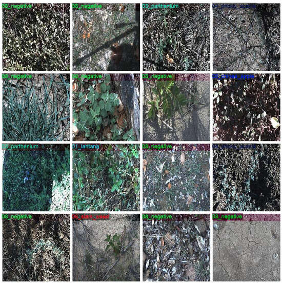
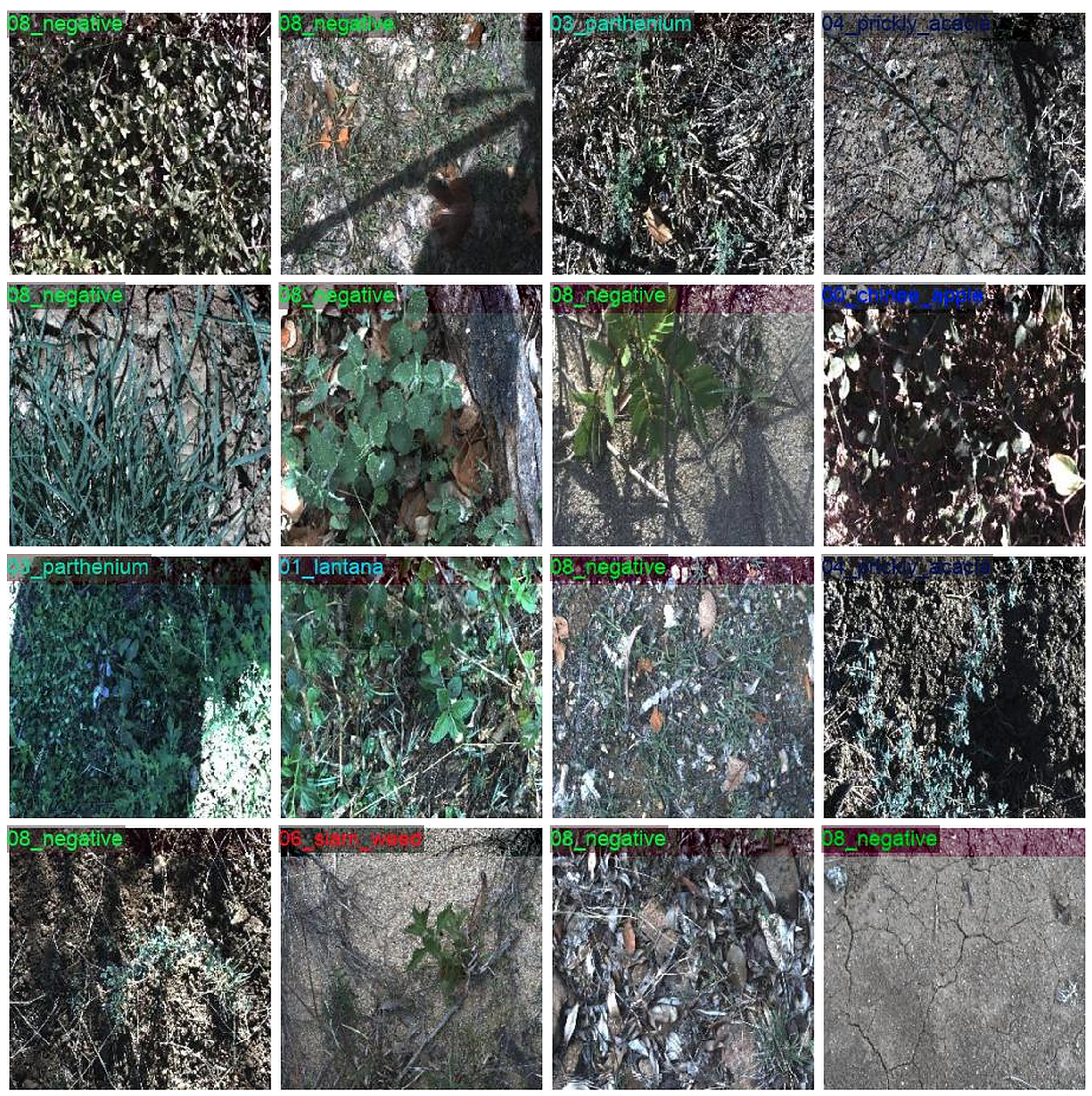
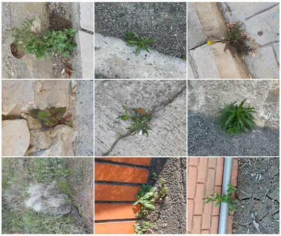
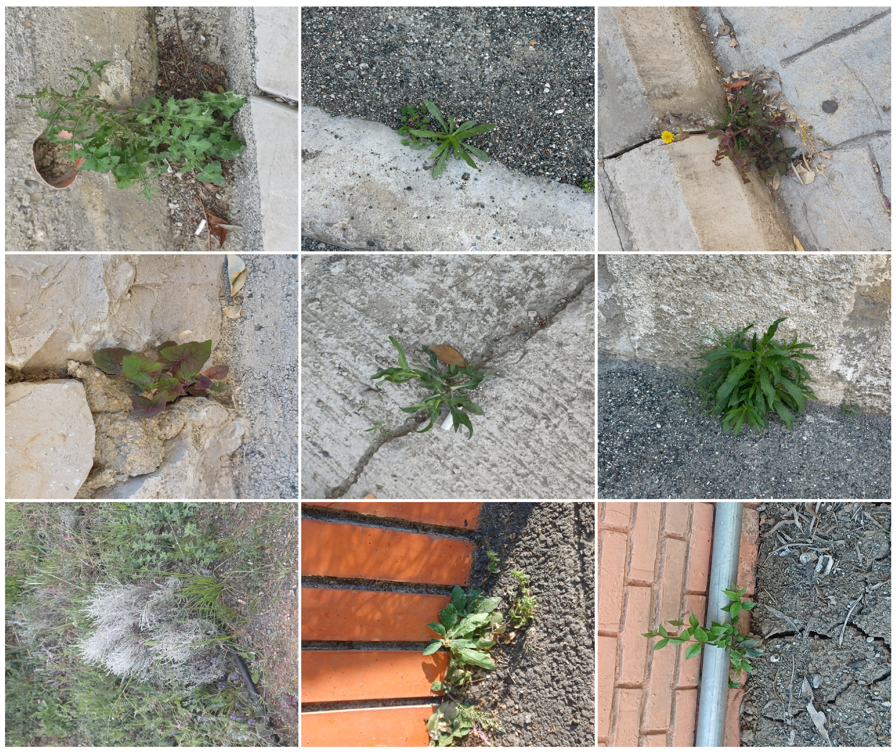
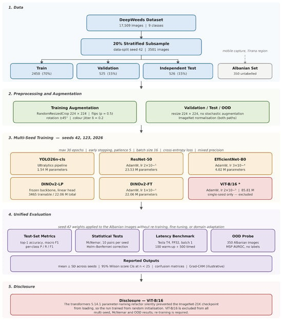
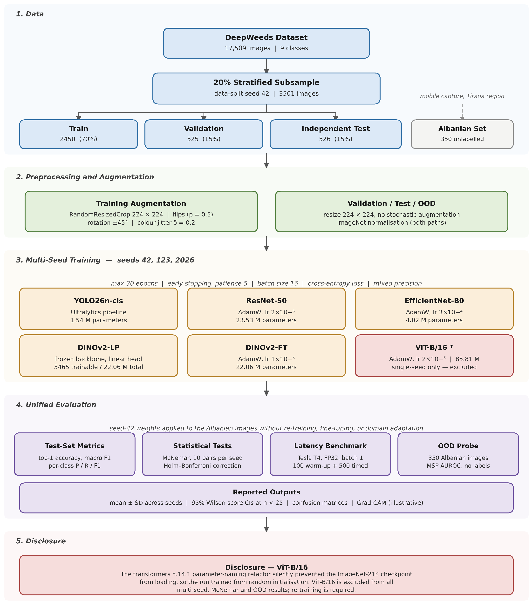
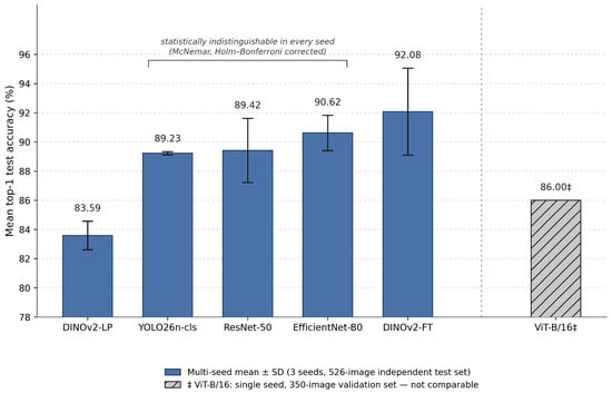
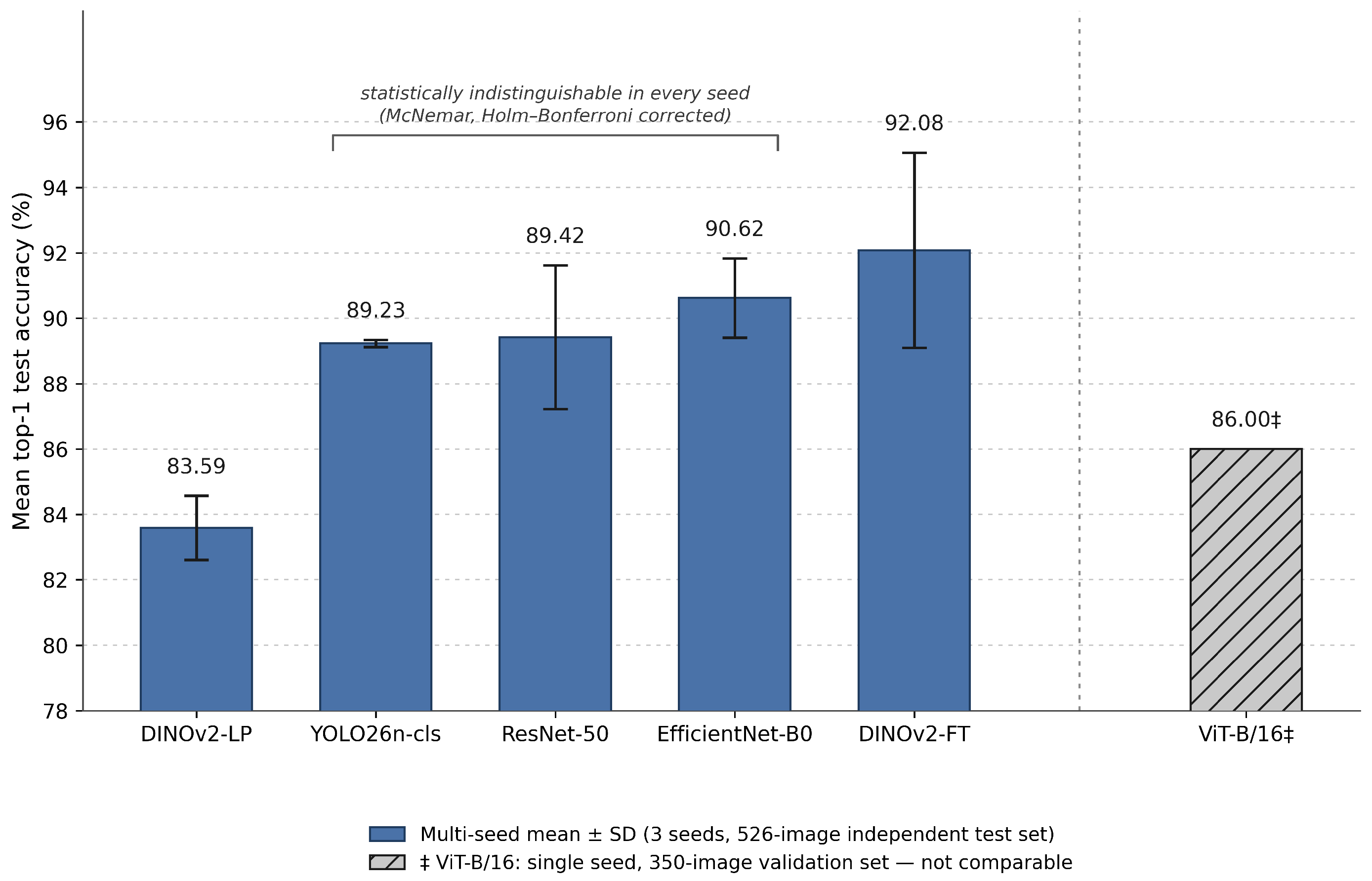
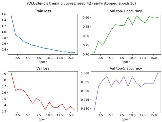
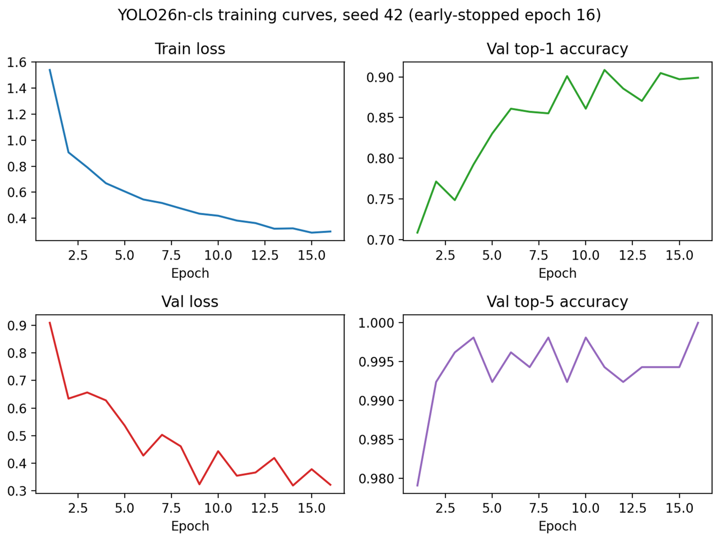
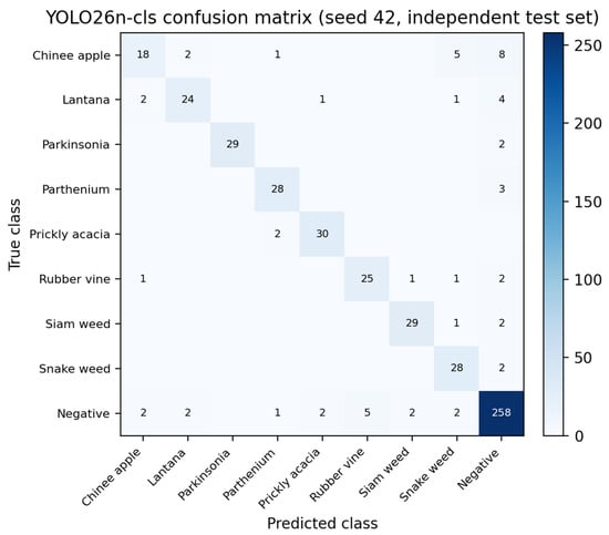
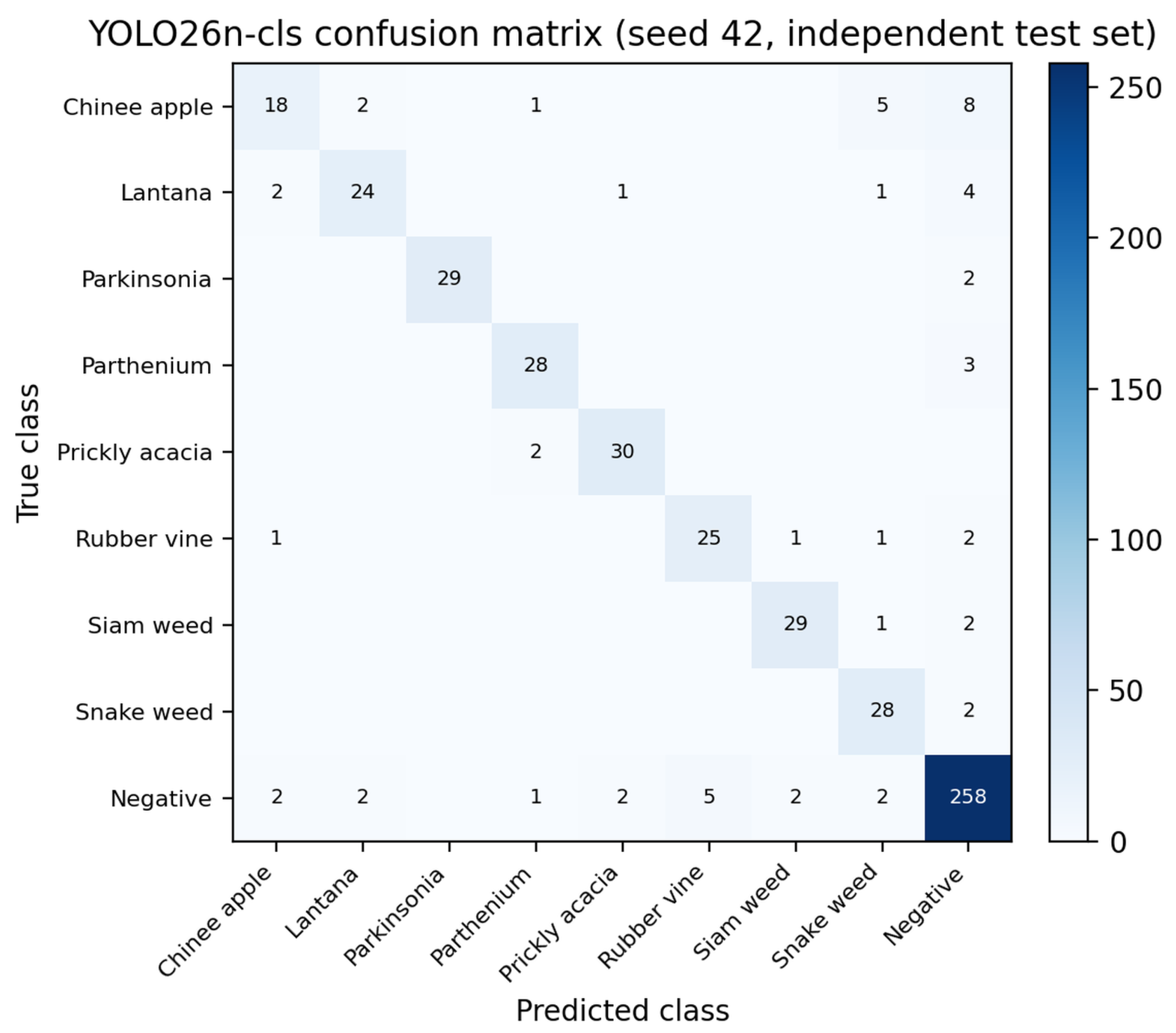
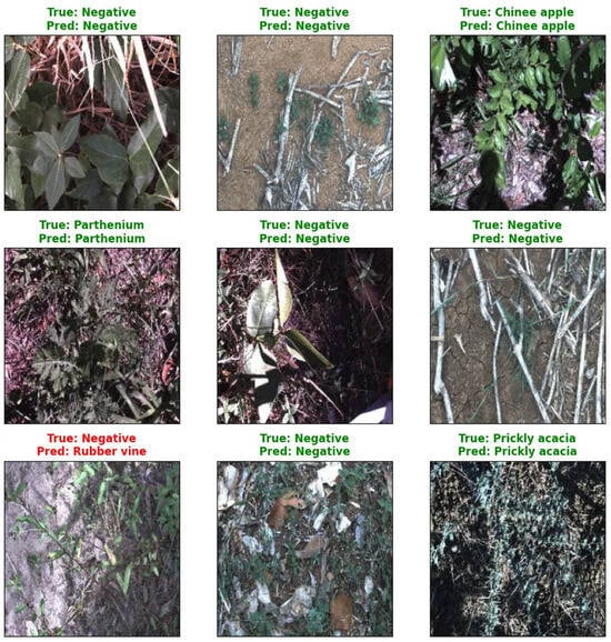
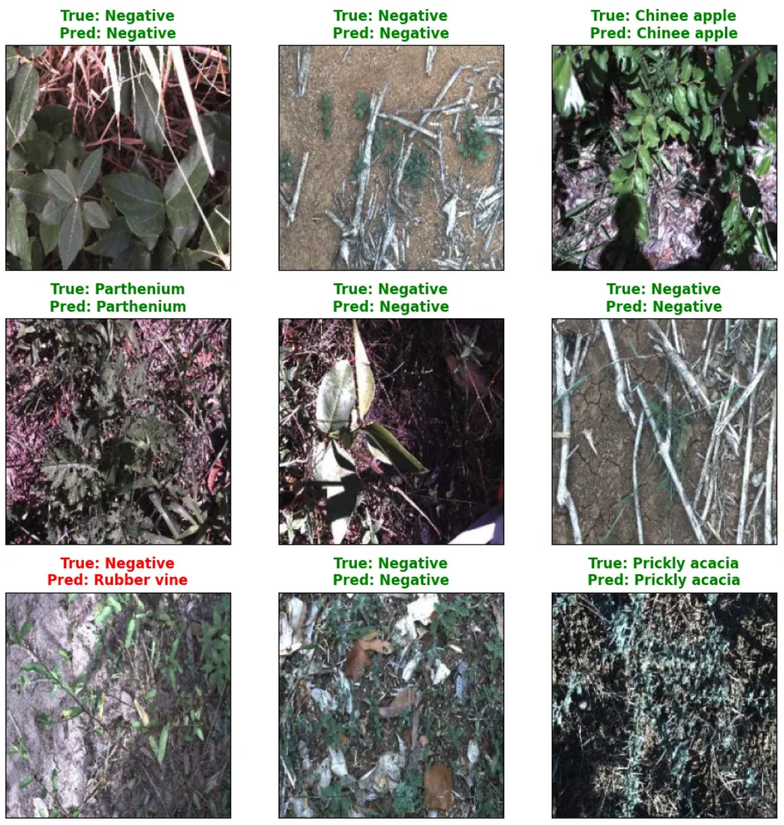
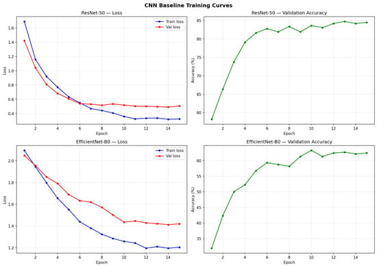
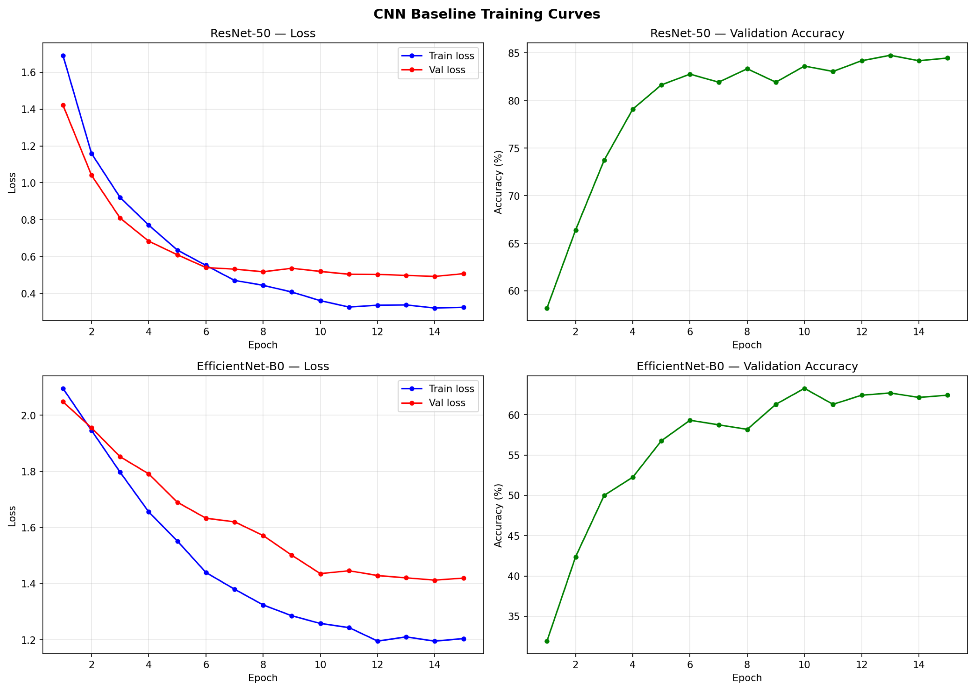
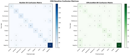
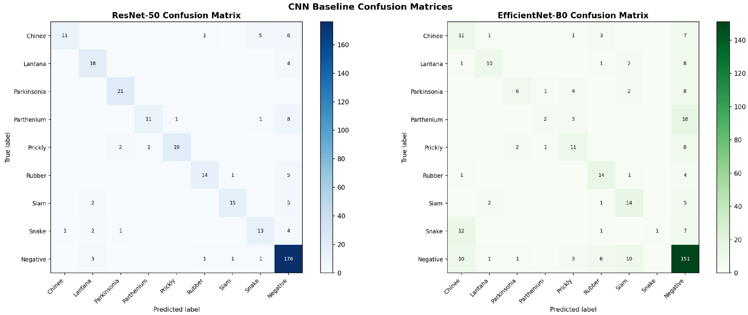
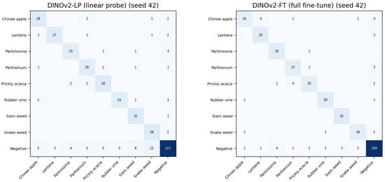
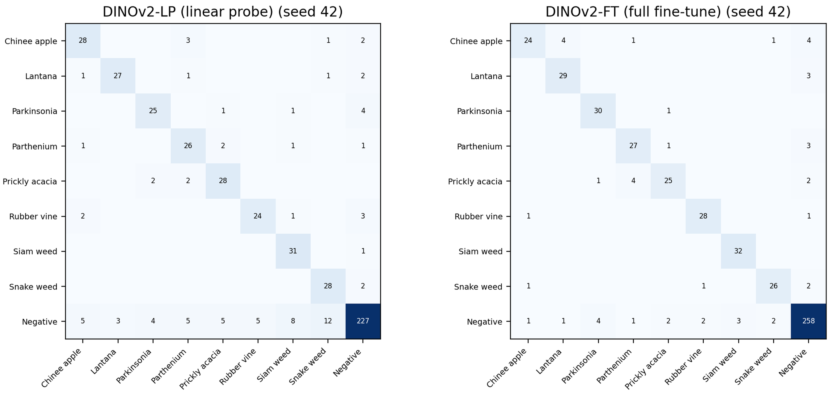
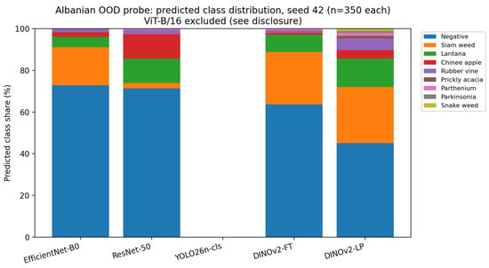
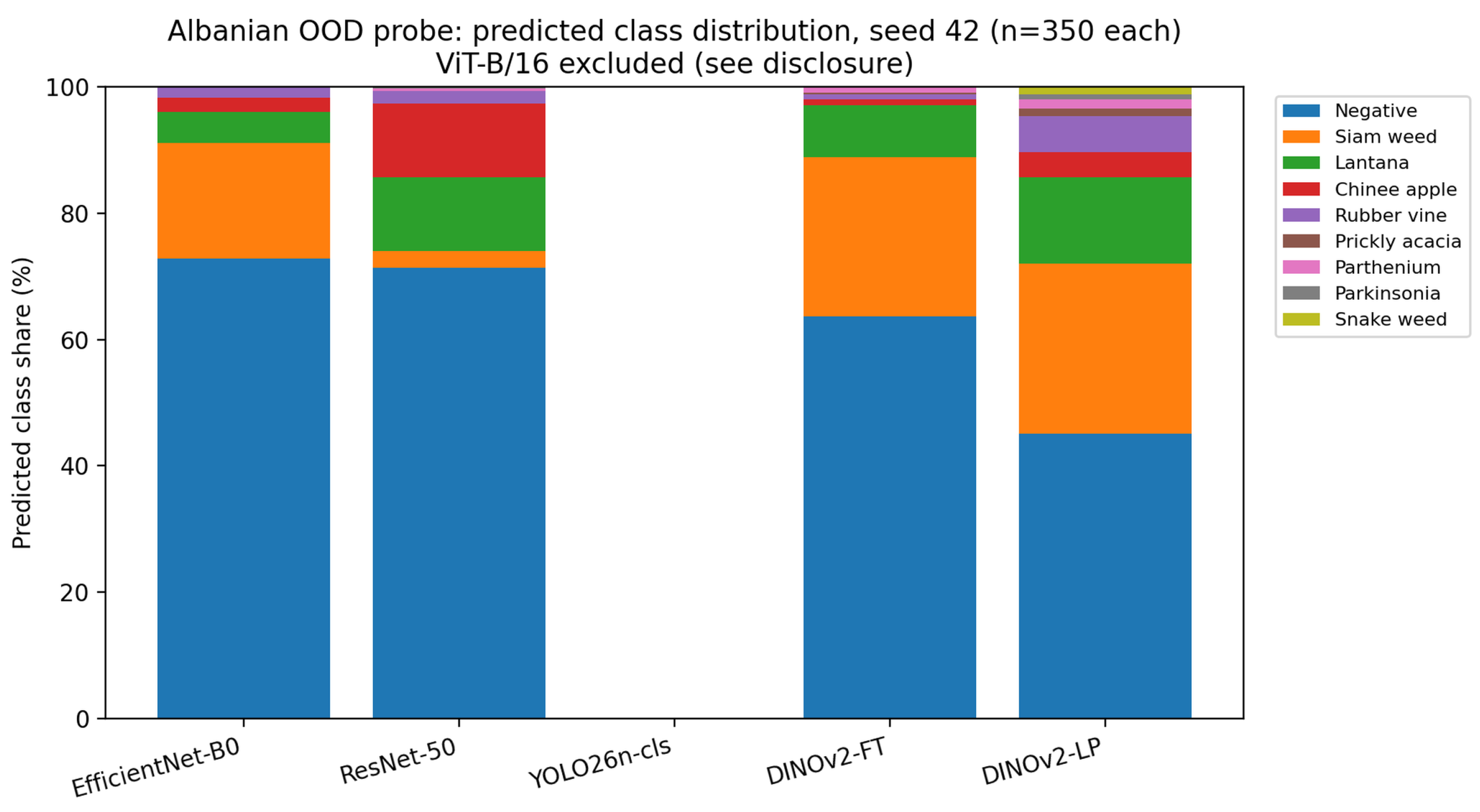

Disclaimer/Publisher’s Note: The statements, opinions and data contained in all publications are solely those of the individual author(s) and contributor(s) and not of MDPI and/or the editor(s). MDPI and/or the editor(s) disclaim responsibility for any injury to people or property resulting from any ideas, methods, instructions or products referred to in the content. |
© 2026 by the authors. Licensee MDPI, Basel, Switzerland. This article is an open access article distributed under the terms and conditions of the Creative Commons Attribution (CC BY) license.