


Abstract
The increasing complexity of next-generation wireless systems challenges the scalability and generalization capabilities of traditional model-driven physical layer (PHY) design, which relies on analytically derived channel models and optimization frameworks. This paper presents a comprehensive survey and critical review of deep learning (DL) architectures enabling the transition toward AI-native PHY design. A unified optimization perspective is developed in which all PHY tasks—including channel estimation, channel state information (CSI) feedback, massive MIMO processing, signal detection, channel coding, beamforming, resource allocation, and semantic-aware transmission—are formulated under a common empirical risk minimization (ERM) framework. Neural architectures such as autoencoders, convolutional and recurrent networks, transformers, and reinforcement learning models are examined through their underlying optimization formulations, loss functions, training methodologies, and representation learning mechanisms. The review compares model-driven and AI-native approaches in terms of performance metrics, computational complexity, robustness, generalization capability, and practical deployment constraints, including hardware limitations, energy efficiency, and real-time feasibility. The analysis highlights the conditions under which AI-native architectures provide adaptability and performance improvements while identifying trade-offs in complexity, latency, and interpretability. The study concludes by outlining prioritized research directions toward fully adaptive and self-optimizing wireless communication systems.
1. Introduction
The evolution of wireless communication systems has been characterized by systematic improvements in capacity, reduced latency, spectral efficiency, and reliability. Earlier generations—from the Third Generation (3G) through the Fourth Generation (4G) and Fifth Generation (5G)—were largely built upon refinements of traditional signal processing techniques and classical information-theoretic principles. However, emerging next-generation wireless systems, particularly those envisioned under the Sixth Generation (6G) umbrella, are increasingly conceived as architectures in which Artificial Intelligence (AI) is tightly integrated across multiple layers of the communication protocol stack, with particular emphasis on the physical layer (PHY) [1,2]. This transition reflects a broader move from strictly model-driven frameworks toward what the research community now terms AI-native system design—a design philosophy in which learning-based components are not merely adjuncts to conventional processing blocks but serve as first-class architectural elements optimized jointly across the entire transmission–reception chain.
Traditionally, the wireless physical layer has been developed through analytical approaches grounded in explicit propagation channel models, statistical signal representations, and optimization techniques derived from convex or structured mathematical formulations. While these model-based methods have achieved remarkable success—enabling, for example, near-capacity-achieving turbo codes and Low-Density Parity-Check (LDPC) decoders—they face fundamental limitations when addressing highly complex communication environments. In particular, high-dimensional Massive Multiple-Input Multiple-Output (MIMO) configurations, Reconfigurable Intelligent Surfaces (RIS), nonlinear channel behaviours, and stringent latency constraints render analytically tractable solutions increasingly elusive [3]. Under such conditions, deriving accurate closed-form solutions or computationally feasible estimators becomes prohibitively difficult.
In this context, Deep Learning (DL) techniques have emerged as a compelling alternative, capable of learning high-dimensional representations and nonlinear mappings directly from data without relying on simplified or inaccurate channel assumptions. By enabling end-to-end optimization, implicit channel modelling, and adaptive signal processing, DL architectures underpin the development of AI-native physical layer designs that fundamentally reshape conventional block-based communication architectures.
Scope and nature of this work. This article constitutes a comprehensive survey and critical review of the state of the art in deep learning for the wireless physical layer. It does not propose a new model, framework, or algorithm; rather, it systematically synthesizes, categorizes, and critically evaluates the existing body of research, identifies open challenges, and delineates future research directions. In doing so, it provides a unified mathematical notation and optimization perspective that connects disparate works spanning channel estimation, signal detection, beamforming, resource allocation, coding, modulation, and semantic communications.
1.1. Contributions of This Article
This survey presents the following principal contributions:
- Unified optimization perspective across all PHY tasks. Unlike prior surveys that treat individual physical layer functions in isolation, this work develops a unified optimization paradigm in which channel estimation, signal detection, beamforming, resource allocation, coding, and modulation are all formulated under a common empirical risk minimization (ERM) framework. This unified viewpoint reveals structural commonalities among seemingly disparate tasks—such as the shared role of encoder–decoder architectures in both autoencoder-based modulation and learned channel estimation—and provides a principled basis for end-to-end system optimization.
- Structured analysis of deep neural network architectures applied to key PHY components, supported by rigorous mathematical formulations, clearly defined objective functions, and explicit optimization constraints.
- Systematic review of learning-based techniques for channel estimation, Channel State Information (CSI) feedback compression, Massive MIMO detection, channel coding, beamforming, and resource allocation, organized by both architectural paradigm and application domain.
- Formal examination of loss functions, training paradigms, and optimization frameworks underlying AI-driven communication systems, including supervised, unsupervised, self-supervised, and reinforcement learning approaches.
- Comparative discussion of model-driven and AI-native approaches in terms of achievable performance, computational complexity, generalization capability, and robustness to model mismatch.
- Critical analysis of implementation challenges, including computational latency, hardware acceleration on Field-Programmable Gate Arrays (FPGAs) and Application-Specific Integrated Circuits (ASICs), adversarial robustness, scalability, and interoperability within Third Generation Partnership Project (3GPP) Release 18/19 [4] and International Telecommunication Union Radiocommunication Sector (ITU-R) International Mobile Telecommunications 2030 (IMT-2030) [5] standardization frameworks.
- End-to-end mathematical consistency. All equations, loss functions, and optimization formulations are presented in a unified and internally consistent notation—with boldface for vectors and matrices—thereby advancing beyond the fragmented treatments found in Huang et al. [6] and Letaief et al. [7], which address network architecture and roadmap visions, respectively, but do not provide the level of mathematical detail and cross-task consistency offered here.
1.2. Novelty and Differentiation from Existing Surveys
The literature on deep learning for wireless communications has grown substantially since the seminal contribution of O’Shea and Hoydis [8], who introduced the autoencoder interpretation of end-to-end communication system design. Subsequent surveys by Qin et al. [9] and Zhang et al. [10] provided valuable overviews of DL applications across different PHY subsystems. While these works laid important groundwork, the present survey is distinguished from them along several critical dimensions:
Compared with O’Shea and Hoydis (2017) [8]: The pioneering work in [8] introduced the concept of modelling the communication system as an autoencoder and demonstrated the feasibility for simple channel models. However, it did not address the breadth of PHY tasks covered here (e.g., Massive MIMO detection, RIS-assisted beamforming, semantic communications) nor did it provide the unified mathematical formulation linking all subsystems under a common optimization framework. The present survey extends that foundational insight to a comprehensive taxonomy spanning seven major PHY domains.
Compared with Qin et al. (2019) [9]: The survey in [9] offered a concise tutorial on DL applications in physical layer communications, covering channel estimation, signal detection, and end-to-end learning. However, it did not include reinforcement-learning-based resource allocation, semantic and task-oriented communications, or hardware implementation analysis. Moreover, the mathematical treatment in [9] was primarily illustrative rather than rigorous. In contrast, the present work provides complete problem formulations with explicit objective functions, constraints, and solution methodologies for each PHY subsystem.
Compared with Zhang et al. (2020) [10]: Ref. [10] focused on AI for 5G and Beyond-5G (B5G) from a circuits and systems perspective, emphasizing implementation efficiency and hardware optimization. While that perspective is valuable, it did not systematically address the information-theoretic foundations of AI-native design, the connection between ERM and mutual information maximization, or the emerging domain of semantic communications. The present survey integrates these theoretical foundations with practical implementation considerations.
Compared with Huang et al. [6] and Letaief et al. [7]: These works presented visionary roadmaps for green 6G networks and AI-empowered wireless systems, respectively. While they provided high-level architectural perspectives, neither offered the detailed mathematical formulations, per-subsystem optimization analyses, or the unified notation framework that characterizes the present survey.
In summary, the key differentiators of this survey are: (i) completeness of PHY coverage spanning all major subsystems within a single, self-contained article; (ii) a unified mathematical notation and optimization framework that links all subsystems; (iii) explicit hardware implementation analysis including FPGA/ASIC deployment considerations; (iv) information-theoretic grounding connecting empirical risk minimization to mutual information maximization and the Information Bottleneck principle; and (v) positioning within current standardization efforts, including 3GPP Release 18/19 and ITU-R IMT-2030.
1.3. Motivation for AI in the Physical Layer
The integration of AI and DL into the wireless physical layer is motivated by several converging factors. Modern communication channels—particularly in millimetre-wave (mmWave) and terahertz (THz) frequency bands—exhibit highly complex propagation characteristics, including severe fading, dynamic blockage, nonlinear dispersion, and atmospheric absorption effects that are difficult to model analytically. Additionally, Mmassive MIMO systems with hundreds or thousands of antennas generate extremely high-dimensional signal spaces in which classical optimization methods become computationally intractable.
Next-generation wireless systems further require real-time adaptation to rapidly varying channel conditions, heterogeneous traffic patterns, and diverse Quality-of-Service (QoS) requirements. Traditional block-wise optimization—whereby the transmitter and receiver components are designed independently—may lead to globally suboptimal performance. In contrast, deep neural networks enable joint end-to-end optimization of the entire transmission–reception chain. Moreover, DL architectures are capable of discovering latent statistical regularities in channel data that are not explicitly captured by simplified analytical models, enabling improved adaptability and robustness.
The system model that underlies the AI-native PHY design philosophy can be stated formally as follows. Consider a discrete-time baseband communication system in which a transmitter encodes a message into a transmitted signal vector , which propagates through a stochastic channel characterized by the conditional distribution , where denotes the channel matrix with transmit and receive antennas, and is the received signal vector. The system is subject to an average transmit power constraint and must operate within a prescribed latency budget and a target error probability . The fundamental objective is to design encoding and decoding functions that maximize the rate of reliable information transfer under these constraints.
1.3.1. Information-Theoretic Foundations of AI-Native PHY
From an information-theoretic perspective, the physical layer aims to reliably transmit a random message across a stochastic channel subject to physical constraints. According to Shannon’s channel coding theorem [11], reliable communication is achievable whenever the transmission rate satisfies:
where denotes the mutual information between transmitted and received signals, is the entropy of the received signal, and is the conditional entropy representing residual uncertainty due to channel noise.
Traditional model-driven designs attempt to approach this theoretical bound through analytically derived modulation schemes, channel codes, and optimal detection rules. However, in highly nonlinear, high-dimensional, or poorly modelled channels—such as those encountered in mmWave, THz, and RIS-assisted environments—explicitly deriving capacity-achieving input distributions and optimal decoders becomes analytically intractable.
Connection between Empirical Risk Minimization and Mutual Information Maximization. AI-native approaches reinterpret the communication chain as a parametric mapping optimized through Empirical Risk Minimization (ERM). To understand this connection intuitively, consider that the goal of a communication system is to maximize the mutual information between the transmitted and received signals—that is, to ensure that the received signal carries as much information as possible about what was sent. In an end-to-end autoencoder formulation [5,6], the transmitter (encoder) and receiver (decoder) are jointly parameterized by neural networks with parameters and , respectively. The system is trained by minimizing the empirical risk:
where is a task-appropriate loss function (e.g., categorical cross-entropy for symbol detection), is the -th transmitted message, and is the decoder output.
The key insight linking ERM to information theory is the following: when the loss function is chosen as the cross-entropy, minimizing Equation (2) is equivalent to minimizing the conditional entropy —that is, the uncertainty about the transmitted message given the decoder output. Since the mutual information can be decomposed as , and is fixed by the source distribution, minimizing the cross-entropy loss directly maximizes the mutual information between the transmitted message and its reconstruction. Thus, the data-driven ERM objective implicitly pursues the same goal as the classical information-theoretic design criterion, but without requiring knowledge of the channel distribution in closed form.
The Information Bottleneck Principle in Wireless PHY. Beyond the direct ERM–mutual information connection, the Information Bottleneck (IB) framework [12] provides a powerful conceptual and mathematical tool for understanding intermediate neural representations in AI-native communication systems. The IB principle formalizes the fundamental trade-off between compression and relevance in learned representations. Specifically, for an intermediate representation of the input , the IB objective seeks to solve:
where measures the complexity of the representation (how much information from the raw input is retained), measures the relevance of the representation (how much information about the task-relevant variable is preserved), and is a Lagrange multiplier controlling the trade-off.
In the context of the wireless physical layer, the IB principle has direct and practical implications. At the transmitter, the encoder must compress the source message into a transmitted signal that fits within the available bandwidth and power budget—this corresponds to minimizing . Simultaneously, the encoded signal must preserve sufficient information for the receiver to reliably decode the intended message—this corresponds to maximizing . Neural network layers in an autoencoder-based communication system naturally perform successive compression-and-refinement operations that approximate the IB optimal trade-off: early layers extract broad features while deeper layers distil task-relevant information and discard channel-induced redundancy.
This perspective is especially pertinent to semantic and task-oriented communications, where the goal is not to reconstruct every transmitted bit perfectly but rather to convey task-relevant meaning. The IB framework provides the theoretical justification for discarding source information that is irrelevant to the downstream task, thereby achieving higher effective throughput. Recent work by Cai et al. [13] has formalized an end-to-end information-theoretic framework for task-oriented semantic communications over MIMO channels, demonstrating that IB-based optimization can yield significant gains in task performance relative to conventional bit-level transmission strategies. In practical wireless applications, the IB perspective supports the design of adaptive modulation, neural decoding, and intelligent beamforming strategies capable of operating near information-theoretic limits without requiring explicit channel models.
1.3.2. Transition from Model-Driven to AI-Native Design
The conventional physical layer is constructed through functional decomposition into independent processing blocks: source coding, channel coding, modulation, equalization, demodulation, and decoding. Each block is optimized separately according to theoretical channel models and criteria such as minimizing the Bit Error Rate (BER) or maximizing Shannon capacity. While this modular approach simplifies design and analysis, it foregoes potential gains from joint optimization across blocks.
Mathematically, consider the standard discrete-time baseband MIMO system model:
where is the transmitted symbol vector, is the MIMO channel matrix capturing path loss, fading, and spatial correlation, is complex Additive White Gaussian Noise (AWGN), and is the received signal vector. The system operates under the constraints:
where denotes the maximum average transmit power, is the input covariance matrix, and denotes the conjugate transpose.
In the traditional paradigm, the transmitter and receiver are designed as separate functions:
where denotes the information bits, is a channel estimate obtained through pilot-based training, and represents the decoded bits. The functions and are independently designed—for example, may implement a combination of LDPC encoding and Quadrature Amplitude Modulation (QAM) mapping, while may cascade a Minimum Mean-Square Error (MMSE) equalizer with a Viterbi decoder.
In contrast, the AI-native approach models the entire communication chain as parameterized neural network mappings and , jointly optimized end-to-end:
subject to , where is a differentiable loss function (e.g., categorical cross-entropy for classification or mean squared error for regression), and the expectation is taken over the joint distribution of messages, channel realizations, and noise. This formulation reframes communication system design as an ERM problem, enabling representation learning directly from data rather than relying exclusively on analytically derived channel models. By jointly optimizing and , the AI-native approach can discover encoding and decoding strategies that exploit channel structure in ways that are inaccessible to conventional block-wise design.
1.4. Comparison with Related Surveys
The depth of coverage, mathematical rigor, and specific PHY subsystems addressed in this survey are carefully differentiated from prior review works in the field. Table 1 provides a structured comparison across the dimensions most relevant to AI-native PHY design.
Table 1.
Comparison of this survey with related reviews on deep learning for the wireless physical layer. Dimensions include coverage of PHY subsystems (channel estimation, Massive MIMO detection, channel coding, beamforming, semantic communications), mathematical formulation depth, hardware implementation analysis, and alignment with standardization frameworks.
This survey is distinguished from prior works by: (i) complete coverage of all major PHY subsystems—channel estimation, Massive MIMO detection, channel coding, beamforming, resource allocation, modulation, and semantic communications—within a single article; (ii) a unified mathematical notation linking all subsystems under a common ERM-based optimization framework; (iii) explicit hardware implementation analysis including FPGA/ASIC deployment considerations and computational complexity profiling; (iv) corrected and complete equation sets presented in consistent notation for all methods; and (v) positioning within 3GPP Release 18/19 and ITU-R IMT-2030 standardization frameworks.
1.5. Organization of the Article
The remainder of this article is structured as follows. Section 2 presents the fundamental deep learning architectures employed in physical layer design, providing the necessary background on Deep Neural Networks (DNNs), Convolutional Neural Networks (CNNs), Recurrent Neural Networks (RNNs), Long Short-Term Memory (LSTM) networks, autoencoders, Generative Adversarial Networks (GANs), transformers, and Deep Reinforcement Learning (DRL). Section 3 reviews AI-based channel estimation and prediction techniques, covering problem formulations, DL architectures, channel sparsity exploitation, and pilot-free methods. Section 4 discusses signal detection using neural networks in MIMO systems. Section 5 examines intelligent beamforming and beam management, including beam prediction, tracking, multi-user beamforming, and RIS-assisted configurations. Section 6 analyses spectral resource management using reinforcement learning, covering Markov Decision Process (MDP) formulations, Deep Q-Networks (DQN), policy gradient methods, and Multi-Agent Reinforcement Learning (MARL). Section 7 presents adaptive modulation and intelligent waveforms, including neural constellation design and Peak-to-Average Power Ratio (PAPR) reduction. Section 8 explores semantic and task-oriented communications, addressing semantic extraction, end-to-end semantic transceivers, and goal-oriented communication. Section 9 discusses implementation challenges and practical considerations, including computational complexity, hardware acceleration, adversarial robustness, and standardization. Section 10 outlines future research directions and emerging trends. Finally, Section 11 presents the conclusions of this survey.
2. Fundamental Deep Learning Architectures for the Physical Layer
This section provides a self-contained overview of the fundamental deep learning architectures that are employed throughout the physical layer applications surveyed in subsequent sections. While the reader is assumed to have a general familiarity with machine learning concepts, this background section establishes the notation, architectural details, and mathematical formulations that will be referenced consistently in Section 3, Section 4, Section 5, Section 6, Section 7 and Section 8. Each architecture is presented with its canonical mathematical description and its particular relevance to wireless PHY tasks is highlighted.
Figure 1 illustrates the principal neural network families—feedforward DNNs, CNNs, RNNs/LSTMs, autoencoders, GANs, transformers, and DRL agents—and their typical mapping to PHY tasks such as channel estimation, signal detection, beamforming, and resource allocation. Key insight: different architectures exploit different structural priors (spatial locality for CNNs, temporal dependencies for RNNs, compression–reconstruction for autoencoders), and the choice of architecture should be guided by the underlying signal processing task. Takeaway: no single architecture dominates across all PHY domains; rather, the optimal choice depends on the dimensionality, temporal dynamics, and optimization objective of the specific application.
Figure 1.
Overview of deep learning architectures for the wireless physical layer.
2.1. Feedforward Deep Neural Networks (DNNs)
Feedforward DNNs constitute the most fundamental deep learning architecture and serve as universal function approximators. For symbol detection and other classification-oriented PHY tasks, a fully connected network maps received signals to symbol probabilities through a sequence of affine transformations and nonlinear activations.
Consider a DNN with hidden layers. The forward pass is defined recursively as:
where is the received signal vector, and are the weight matrix and bias vector of the -th layer, denotes a nonlinear activation function such as the Rectified Linear Unit (ReLU) or hyperbolic tangent (tanh), and is the output probability vector over the symbol alphabet. In PHY applications, DNNs are used for tasks including symbol detection [14], CSI feedback compression, and power control, where the mapping from input features to output decisions can be learned directly from training data.
2.2. Convolutional Neural Networks (CNNs)
CNNs exploit spatial or temporal structure in signals through convolution operations with shared, shift-invariant parameters. For a one-dimensional input signal , the convolution operation at the -th layer is defined as:
where the index represents temporal or spatial displacement, and are the learned filter coefficients. CNNs are particularly effective for processing temporal symbol sequences and for exploiting spatial correlation in antenna arrays. In the context of channel estimation, two-dimensional CNNs can process the time-frequency channel response as an image-like structure, enabling denoising and interpolation that leverage the inherent correlation structure of wireless channels [15].
2.3. Recurrent Neural Networks (RNNs) and LSTMs
For modelling temporal channel evolution—such as time-varying fading or Doppler-induced variations—Recurrent Neural Networks maintain a hidden state that captures temporal dependencies. The standard RNN update is:
where is the hidden state at time step , is the input at time , and , , are learnable parameters.
Long Short-Term Memory (LSTM) architectures extend the basic RNN with gating mechanisms that mitigate the vanishing gradient problem and enable modelling of long-range temporal dependencies:
where , , and denote the forget, input, and output gates, respectively, represents the cell state, is the sigmoid activation function, and denotes element-wise (Hadamard) multiplication. In wireless PHY applications, LSTM networks are employed for channel prediction in time-varying environments [16], enabling proactive resource allocation and predictive beamforming.
2.4. Autoencoders (AEs)
The communication system can be holistically modelled as a learned encoder–channel–decoder structure, following the autoencoder interpretation introduced by O’Shea and Hoydis [8]. The encoder maps a message to a transmitted signal, the signal passes through the physical channel, and the decoder reconstructs the message:
where is the neural encoder and is the neural decoder. The objective is to minimize the reconstruction loss:
Variational Autoencoders (VAEs) incorporate probabilistic regularization by introducing a latent variable and optimizing the Evidence Lower Bound (ELBO):
where denotes the Kullback–Leibler divergence, serving as a regularization term that encourages the learned latent distribution to remain close to a tractable prior . In PHY applications, autoencoders enable end-to-end learning of modulation, coding, and signal shaping strategies that are jointly optimized for the channel [8,17].
2.5. Generative Adversarial Networks (GANs)
GANs provide a framework for learning to generate realistic synthetic data and are employed in wireless communications primarily for channel modelling and data augmentation. A GAN consists of two competing networks—a generator and a discriminator —trained via the minimax objective:
The generator is trained to produce synthetic channel realizations that are statistically indistinguishable from real channel samples as evaluated by the discriminator . At convergence, the generator implicitly learns the underlying channel distribution , enabling applications such as channel simulation for training data augmentation, domain adaptation across deployment environments, and stochastic channel modelling without closed-form distribution assumptions.
2.6. Transformers and Attention Mechanisms
Originally developed for Natural Language Processing (NLP) tasks, transformer architectures have been extended to wireless signal processing applications through self-attention mechanisms that capture long-range dependencies without the sequential processing bottleneck of RNNs. The scaled dot-product attention is computed as:
where , , and denote the query, key, and value matrices obtained from the input signals via learned linear projections, and is the dimensionality of the key vectors. The scaling factor prevents the dot products from growing excessively large in high-dimensional spaces.
Transformer architectures are particularly effective in modelling long-range temporal dependencies and spatial correlations in Massive MIMO systems [18]. Multi-head attention further enhances representational capacity by computing multiple attention functions in parallel and concatenating their outputs, enabling the model to attend to information from different representation subspaces simultaneously.
2.7. Deep Reinforcement Learning (DRL)
For sequential decision-making and resource allocation problems where the optimal action depends on the evolving system state, DRL models the system as a Markov Decision Process (MDP) defined by the tuple , where denotes the state space, the action space, the state transition probabilities, the reward function, and the discount factor [19].
The objective is to learn an optimal policy that maximizes the expected cumulative discounted return:
where is the reward obtained at time step under state and action . Algorithms such as Deep Q-Networks (DQN) [20], Policy Gradient methods, Actor–Critic architectures, and Proximal Policy Optimization (PPO) [21] are employed to approximate the optimal policy or the action-value function using neural networks. In wireless PHY applications, DRL is applied to dynamic spectrum access, power control, beam management, and resource scheduling, where the environment evolves stochastically and decisions must be made sequentially under uncertainty [22].
3. AI-Based Channel Estimation and Prediction
Accurate channel estimation constitutes a fundamental prerequisite for coherent wireless communication systems, as it directly governs the performance of subsequent receiver functions including equalization, detection, and Multiple-Input Multiple-Output (MIMO) processing [23]. This section provides a systematic review of Artificial Intelligence (AI)-based channel estimation and prediction techniques that address the limitations of classical model-driven estimators in emerging wireless scenarios. Traditional approaches—such as Least Squares (LS), Minimum Mean Square Error (MMSE), and pilot-assisted methods—are well understood under stationary channel conditions; however, they exhibit fundamental limitations in environments characterized by high user mobility, high-dimensional antenna configurations, and severely constrained pilot resources [24,25]. These limitations are particularly pronounced in systems operating at millimeter-wave (mmWave) and sub-terahertz (sub-THz) frequencies, where propagation channels exhibit sparse multipath structures, rapid temporal variations, and highly directional characteristics. Deep Learning (DL) architectures offer a promising alternative by learning complex, high-dimensional channel representations directly from data, without relying on simplified analytical channel models. This section reviews the problem formulation, representative neural architectures, sparse and pilot-free estimation strategies, transfer and meta-learning techniques, and comparative performance analyses.
Figure 2 conceptually illustrates the channel estimation problem in high-dimensional wireless systems. The estimator must reconstruct the full channel frequency response from limited and noisy pilot observations while exploiting spatial, frequency, and temporal correlations inherent in the propagation environment.
Figure 2.
Channel estimation problem in next-generation wireless systems.
Figure 2 depicts a multi-antenna transmitter–receiver pair operating over a wideband channel with subcarriers and antenna dimensions. Pilot symbols (shown as shaded resource elements) are inserted at sparse locations in the time–frequency grid, while the estimator must infer the full channel state information (CSI) across all resource elements. The key insight is that AI-native estimators exploit learned spatial, frequency, and temporal correlations to interpolate channel coefficients at non-pilot positions with substantially lower mean square error (MSE) than classical LS or MMSE methods, particularly under low signal-to-noise ratio (SNR) and limited pilot density conditions. The takeaway is that neural architectures can adaptively learn channel statistics from data, enabling robust estimation without requiring explicit knowledge of channel covariance matrices or stationarity assumptions.
3.1. Problem Formulation
Consider a multi-carrier Orthogonal Frequency Division Multiplexing (OFDM) or Orthogonal Frequency Division Multiple Access (OFDMA) system with subcarriers, transmit antennas, and receive antennas. The received signal at subcarrier and time index is expressed as:
where denotes the channel frequency response matrix, represents the transmitted symbol vector, and is additive white Gaussian noise (AWGN). The channel estimation problem consists of recovering from the observations at known pilot positions and, potentially, from previously detected data symbols.
- System Model Assumptions and Constraints. The system model in (25) assumes a block-fading channel that remains approximately constant over each OFDM symbol but may vary across symbols. The pilot overhead is constrained by a fraction of total subcarriers allocated to pilots, where denotes the number of pilot subcarriers. The fundamental objective is to minimize the normalized mean square error (NMSE):subject to constraints on pilot density, computational complexity, and latency.
- Traditional LS Estimation. At pilot positions where is known, the LS estimate is given by , where denotes the Moore–Penrose pseudo-inverse. The LS estimator does not require statistical knowledge of the channel; however, it exhibits high MSE under low SNR conditions due to noise amplification, and it does not exploit inter-subcarrier or inter-antenna correlations.
- Traditional MMSE Estimation. The MMSE estimator minimizes the expected MSE:where is the channel covariance matrix. Although MMSE yields the optimal linear estimate under Gaussian assumptions, it requires knowledge of second-order channel statistics , which may be non-stationary in dynamic environments, and involves matrix inversion with cubic complexity , rendering it computationally prohibitive for massive MIMO configurations.
3.2. Deep Learning Architectures for Channel Estimation
DL-based approaches reinterpret channel estimation as a supervised regression problem, where a neural network learns the mapping from noisy observations to channel coefficients:
with parameters optimized by minimizing the empirical risk:
where denotes the training dataset comprising input–output pairs of pilot observations and ground-truth channel realizations. Unlike LS and MMSE estimators, neural estimators implicitly learn channel statistics from data without requiring explicit covariance matrices. We review the principal architectures below. Fully Connected Networks (FCNs). Deep Neural Network (DNN)-based estimators directly map pilot observations to channel coefficients through successive fully connected layers. While effective in moderate dimensions, the parameter count scales as , which limits their applicability to large-scale MIMO systems. FCN estimators typically serve as baseline architectures for benchmarking more structured designs.
- Convolutional Neural Network (CNN)-Based Estimators. Wireless channels exhibit spatial correlations across antennas and frequency correlations across subcarriers. CNNs exploit this structure through shared convolutional kernels:where denotes the convolution operation, and are the learnable kernel weights and biases of layer , and is a nonlinear activation function. CNN-based architectures—including residual networks (ResNets) and densely connected networks—have demonstrated improved NMSE under spatially correlated channel conditions by leveraging parameter sharing and translation equivariance. The weight-sharing property reduces the total parameter count by orders of magnitude compared to FCNs, yielding complexity where is the kernel size, are input/output channels, and is the number of layers.
Transformer-Based Estimators. Transformers capture long-range dependencies across subcarriers and antenna elements through self-attention mechanisms, without imposing fixed convolutional receptive fields:
where , , and denote the query, key, and value matrices derived from the input via learned linear projections, and is the key dimension. Self-attention dynamically weights contributions from different subcarriers or antenna elements, enabling adaptive estimation across frequency bands and spatial dimensions. Transformer-based estimators are particularly effective in wideband massive MIMO systems where channel correlations span large frequency–spatial regions [18]. The computational complexity per attention layer is , which may be reduced through sparse or linear attention approximations.
- Generative Adversarial Network (GAN)-Assisted Refinement. GAN-based approaches refine coarse initial estimates (e.g., from LS) by training a generator network to produce realistic channel estimates that are indistinguishable from true channel realizations as judged by a discriminator network :
A reconstruction term ensures estimation fidelity:
These approaches are particularly relevant in pilot-scarce regimes, where the generator implicitly learns the channel distribution and uses this prior to denoise coarse estimates. However, GAN training introduces additional complexity due to the minimax optimization and potential mode collapse, requiring careful hyperparameter tuning.
- Trade-offs in Architecture Selection. The choice among FCN, CNN, Transformer, and GAN architectures involves trade-offs in estimation accuracy, computational complexity, latency, and interpretability. FCNs offer simplicity but poor scalability; CNNs provide an effective balance of accuracy and efficiency through parameter sharing; Transformers achieve the highest accuracy for large-scale systems at the cost of quadratic attention complexity; and GANs excel in low-pilot scenarios but introduce training instability. Practical deployment must consider hardware constraints, inference latency budgets (e.g., sub-millisecond for Ultra-Reliable Low-Latency Communication (URLLC) applications), and energy consumption targets.
3.3. Channel Prediction in Time-Varying Environments
In high-mobility wireless systems and latency-critical applications, channel prediction enables proactive compensation mechanisms and predictive resource scheduling. The temporal evolution of the channel can be modelled as a stochastic process:
where is a nonlinear state-transition function, is the memory depth, and represents stochastic innovation noise. Recurrent Neural Network (RNN) and Long Short-Term Memory (LSTM) architectures approximate the prediction function:
with training objective:
Transformer-based sequence models further improve multi-step prediction by capturing long-range temporal dependencies through self-attention across the temporal dimension, enabling more stable predictions over longer horizons [16]. In vehicular scenarios at speeds exceeding 120 km/h, LSTM-based predictors have been shown to reduce multi-step prediction NMSE by 4–6 dB relative to classical autoregressive (AR) models, while attention-augmented architectures provide additional gains of 1–2 dB.
- Real-World Deployment Considerations. Channel prediction requires inference latency shorter than the channel coherence time; for vehicular channels at 28 GHz with Doppler spreads exceeding 1 kHz, the coherence time may be below 1 ms, imposing stringent computational constraints. Model compression techniques—including pruning, quantization, and knowledge distillation—are essential for real-time deployment on edge hardware [26,27].
3.4. Sparse and Pilot-Free Channel Estimation
This subsection consolidates two complementary strategies for reducing pilot overhead: exploiting channel sparsity through compressed sensing and learning-based methods, and blind estimation techniques that eliminate pilot symbols entirely.
3.4.1. Compressed Sensing with Deep Learning
- Millimeter-wave and terahertz channels: Typically exhibit sparse structures in the angular domain due to limited scattering paths. This sparsity can be exploited to reduce estimation overhead and computational complexity. The theory of compressed sensing (CS) establishes that sparse signals can be recovered from sub-Nyquist measurements through -norm optimization:where denotes the sparse angular-domain representation of the channel, is the measurement matrix determined by pilot placement, represents the pilot observations, and bounds the noise level. Neural unfolding methods map iterative CS algorithms (e.g., ISTA, ADMM) into trainable layers:where each iteration of the underlying optimization algorithm is unfolded into a corresponding neural network layer, allowing the model to learn regularization parameters and adaptive thresholding operators jointly from data.
- Learned ISTA (LISTA). A representative example of algorithm unfolding is the Learned Iterative Shrinkage-Thresholding Algorithm:where denotes the soft-thresholding operator:
The parameters , , and are learned for each layer , significantly accelerating convergence (typically 10–20×) compared to classical ISTA while maintaining or improving recovery accuracy. The training loss is:
where is the total number of unfolded layers (iterations).
3.4.2. Pilot-Free Channel Estimation via Deep Learning
Blind channel estimation schemes exploit the inherent structure of data signals to estimate the channel without allocating explicit pilot resources, thereby maximizing spectral efficiency. An autoencoder (AE) architecture can jointly learn encoding, channel estimation, and decoding:
where denotes the information bits, the encoded transmission, and the decoded output. The loss function combines data reconstruction accuracy and channel estimation quality:
where balances the two objectives. The encoder implicitly learns to embed structural redundancy into the transmitted signal, facilitating blind channel recovery at the receiver.
- Deep Blind Equalization. DL extends classical techniques such as the Constant Modulus Algorithm (CMA) by allowing neural networks to learn adaptive cost functions:where is the target constant modulus. Neural networks generalize this criterion to arbitrary constellations and nonlinear channel conditions, providing improved convergence and reduced steady-state error.
3.5. Transfer Learning and Meta-Learning for Channel Estimation
In practical wireless systems, training DL models from scratch for each specific channel scenario—characterized by distinct propagation conditions, carrier frequencies, antenna configurations, and deployment environments—is computationally prohibitive and data-intensive. Transfer learning and meta-learning strategies address this challenge by enabling rapid adaptation to new scenarios using limited target-domain data.
Transfer Learning. A model pre-trained on a diverse set of source–channel scenarios can be adapted to a target scenario through selective fine-tuning of higher network layers, while preserving generalizable low-level feature representations in frozen lower layers. The adapted parameters are obtained by
where denotes the frozen parameters of lower layers and are the trainable parameters of upper layers. This approach typically reduces the required target-domain training samples by 5–10× and adaptation time by an order of magnitude, while preserving generalizable feature representations learned from diverse channel environments.
- Model-Agnostic Meta-Learning (MAML). MAML seeks a parameter initialization that enables rapid adaptation to new tasks (channel scenarios) with only a few gradient updates:
For channel estimation, each task corresponds to a different propagation scenario (e.g., indoor office, urban macro, vehicular highway). MAML learns an initialization that generalizes across diverse channel distributions, enabling efficient adaptation under distribution shifts with as few as 5–10 gradient steps and 50–100 target-domain samples.
- Complexity and Practical Considerations. Transfer learning introduces minimal computational overhead during fine-tuning (typically 1–5% of full training cost), while MAML requires second-order gradient computation during meta-training, increasing training cost by approximately 2–3×. However, both approaches dramatically reduce deployment-time adaptation costs, which is the primary practical concern for real-world systems.
3.6. Performance Evaluation and Comparative Analysis
Extensive empirical studies have compared DL-based channel estimation methods with classical model-driven techniques across a variety of propagation environments [15,16]. The key findings are summarized below, with a structured comparison provided in Table 2.
Table 2.
Comparative Analysis of Channel Estimation and Prediction Methods.
In large-scale MIMO configurations operating at mmWave frequencies, neural architectures consistently demonstrate improved estimation accuracy relative to LS and MMSE, particularly under low SNR conditions and limited pilot resources. In representative massive MIMO scenarios (e.g., 64-antenna arrays under standardized 3GPP 38.901 Urban Micro (UMi) channel models), FCN estimators typically outperform LS by 5–8 dB and MMSE by 3–5 dB in NMSE, while CNN-based architectures further enhance performance by 1–2 dB through exploitation of spatial and frequency-domain correlations. Transformer-based models provide additional gains of 0.5–1.5 dB by capturing long-range dependencies across subcarriers and antenna elements. These improvements are especially pronounced in high-mobility regimes, where model mismatch degrades the effectiveness of classical estimators [15].
For channel prediction in vehicular environments, LSTM networks substantially reduce multi-step prediction error compared to classical AR models. Attention-based transformers further improve prediction stability over longer horizons, enabling proactive CSI acquisition and reducing feedback latency [16].
However, performance gains must be evaluated alongside computational complexity and real-world deployment feasibility. The MMSE estimator scales as due to matrix inversion, whereas DNN complexity depends primarily on network depth and hidden layer width. CNN architectures reduce parameter count through weight sharing, and transformer models introduce attention complexity. Practical deployment therefore requires model compression techniques—including INT8/INT4 quantization, structured pruning, and knowledge distillation—to satisfy latency constraints (sub-millisecond for URLLC) and energy budgets on embedded hardware platforms [26,27].
Overall, while AI-native channel estimators offer improved robustness and adaptability in complex propagation environments, their benefits depend on the availability of representative training data, efficient hardware acceleration, and careful architectural choices that balance accuracy against inference cost.
Table 2 summarizes representative channel estimation and prediction approaches, highlighting trade-offs between statistical assumptions, data dependency, computational complexity, and adaptability across classical and AI-native methods.
4. Signal Detection Using Neural Networks
Signal detection is a critical function of the wireless receiver, responsible for estimating transmitted symbols or information bits from noisy, distorted received signals [30]. In high-dimensional Multiple-Input Multiple-Output (MIMO) systems, optimal Maximum Likelihood (ML) detection exhibits exponential computational complexity in the number of transmit antennas and constellation size, which motivates the development of suboptimal approximations with reduced computational cost [31]. Deep Learning (DL) provides an alternative paradigm by enabling detection architectures that achieve a favourable balance between detection performance and computational complexity through learned, data-adaptive detection structures [14]. This section reviews the detection problem formulation, neural network architectures for direct and structured detection, extensions to non-ideal channels and multi-user scenarios, and implementation considerations.
Figure 3 illustrates the signal detection framework based on DL techniques, depicting the mapping from received signals and Channel State Information (CSI) to detected symbols or bits through a trained neural architecture.
Figure 3.
Signal detection framework based on deep learning techniques.
Figure 3 shows the receiver processing chain in a MIMO system, where the received signal vector and the estimated channel matrix are jointly fed into a neural network detector. The architecture comprises multiple hidden layers with nonlinear activations, producing either hard symbol decisions or soft bit-level log-likelihood ratios (LLRs) at the output. The key insight is that neural detectors learn implicit interference cancellation and noise suppression strategies from training data, achieving near-ML performance at computational costs comparable to linear detectors. The takeaway is that DL-based detection is particularly advantageous in high-dimensional MIMO systems () where the ML complexity becomes prohibitive, offering practical deployment on FPGA and ASIC platforms with sub-10 μs latency.
4.1. Detection Problem Formulation
System Model. Consider the standard MIMO signal model:
where is the received signal vector, is the channel matrix, is the transmitted symbol vector with denoting the signal constellation (e.g., -QAM), and is AWGN. The detection objective is to estimate by minimizing the probability of detection error .
- Maximum Likelihood Detection. The ML detector computes:
The computational complexity is , which grows exponentially with the number of transmit antennas, rendering ML detection infeasible for systems with and higher-order modulations.
- Linear Detectors. Zero-Forcing (ZF) and MMSE detectors provide linear solutions with polynomial complexity :
These detectors exhibit suboptimal performance, particularly under high system loading conditions where , due to residual inter-stream interference that linear processing cannot fully suppress.
4.2. Neural Networks for Direct Detection
- DNN Detector. A direct approach employs a Deep Neural Network to map the received signal and CSI to the detected symbols:where the architecture comprise: Input: Concatenation of real and imaginary parts ; Hidden Layers: Multiple fully connected layers with Rectified Linear Unit (ReLU) activation functions and optional batch normalization; Output: For complex symbol detection: real-valued outputs; for bit detection: outputs with sigmoid activation.
- Loss Functions. For symbol-level detection, the MSE loss is employed:
For bit-level soft-output detection, the binary cross-entropy (BCE) loss is used:
where and denote the true and estimated bit probabilities, respectively.
Training Methodology. Training data are generated by sampling channel realizations from the target channel model (e.g., 3GPP Spatial Channel Model), random symbol vectors from , and noise vectors. The dataset typically comprises – samples, split into training (80%), validation (10%), and test (10%) sets. The Adam optimizer with learning rate scheduling (initial rate , decay factor 0.5 every 50 epochs) is commonly employed.
4.3. Attention and Transformer-Based Detection
- Attention-Based Detection. Attention mechanisms enable the detector to focus on the most relevant components of the received signal for detecting each transmitted symbol:where represents the query used to detect symbol , while and correspond to key and value projections derived from the received signals, and is the projection dimension.
- ✓
- Transformer-Based Detector. A complete transformer-based detection architecture consists of the following elements:
- Embedding: Projection of the received signals into a high-dimensional representation space
- Multi-Head Self-Attention: Captures interdependencies among transmitted symbols across spatial streams
- Feed-Forward Networks: Performs nonlinear feature transformation with residual connections
- Output Layer: Produces symbol probabilities or bit-level LLRs
The computational complexity per transformer layer is , which is significantly more efficient than ML detection for moderate values of (e.g., ). For a MIMO system with 64-QAM, the transformer detector achieves within 0.5 dB of ML performance while reducing complexity by over five orders of magnitude.
4.4. Detection Under Non-Ideal Conditions
- Fading Channels. For time-varying fading channels, the training procedure incorporates channel statistics to build robustness:where represents fading coefficients and denotes element-wise multiplication. The neural detector implicitly learns robustness to fading variations by training over diverse channel realizations, without requiring explicit diversity combining mechanisms.
- Hardware Impairments. Neural detectors can also compensate for hardware imperfections—including in-phase/quadrature (IQ) imbalance, power amplifier (PA) nonlinearities, phase noise, and quantization effects—by learning directly from measured data:where encapsulates the aggregate hardware distortion. The neural detector implicitly learns to invert hardware-induced distortions, enabling improved detection under non-ideal operating conditions that are difficult to model analytically. This capability is particularly valuable for low-cost devices with significant hardware imperfections and for mmWave systems where PA nonlinearities are pronounced.
4.5. Multi-User Detection
- DL-Based Non-Orthogonal Multiple Access (NOMA) Detection. In NOMA systems, multiple users share the same time–frequency resources through power-domain multiplexing. The received signal is:where , , and denote the transmit power, channel vector, and symbol of user , respectively. A neural detector can perform learned successive interference cancellation (SIC):enabling joint multi-user detection by implicitly learning interference structures and decoding order, without relying on explicitly designed SIC procedures.
- Multi-Cell Detection with Graph Neural Networks (GNNs). In multi-cell scenarios with strong inter-cell interference, GNNs model the interference structure by representing each user as a node and interference relationships as edges:where denotes the set of interfering neighbours of user , is the message embedding at layer , and AGG denotes a permutation-invariant aggregation function. The GNN propagates information across the interference graph to enable cooperative interference mitigation with complexity scaling linearly in the number of edges.
4.6. Computational Complexity and Hardware Implementation
- Complexity Comparison. Table 3 summarizes the computational complexity and relative performance of representative detection algorithms, including ML, ZF, MMSE, sphere decoding, DNN, and transformer-based detectors.
Table 3.
Computational complexity and performance trade-offs of model-driven and deep learning-based detectors.
Table 3 compares detection approaches along the dimensions of computational complexity (in floating-point operations), detection performance relative to ML (in dB gap), scalability with , and suitability for hardware acceleration. DL-based detectors occupy a favourable region in the complexity–performance trade-off space, achieving near-ML accuracy with polynomial or fixed complexity.
- FPGA Implementation. Neural detectors are highly parallelizable, making them well suited for hardware acceleration. Field-Programmable Gate Array (FPGA) implementations have demonstrated: throughput exceeding 1 Gbps for MIMO systems, latency below 10 μs, and energy efficiency greater than 100 Mbps/W. These results confirm the feasibility of deploying DL-based detectors in real-time communication systems [32,33].
- Quantization. Model quantization techniques, such as reducing weights and activations to INT8 or INT4 precision, decrease memory footprint and power consumption by factors of 4–8, with minimal performance degradation (typically less than 0.5 dB in Bit Error Rate (BER)) [34]. Post-training quantization and quantization-aware training represent complementary strategies, with the latter yielding smaller accuracy losses at the cost of additional training effort.
- Interpretability Considerations. Unlike classical detectors whose behaviour can be analysed through well-understood algebraic relationships, neural detectors operate as learned nonlinear mappings with limited interpretability. Algorithm unfolding—where iterative detection algorithms (e.g., projected gradient descent, expectation propagation) are mapped to trainable neural layers—provides a principled approach to combining the interpretability of model-driven methods with the adaptability of data-driven learning [14].
5. Intelligent Beamforming and Beam Management
Beamforming is a fundamental technique in Multiple-Input Multiple-Output (MIMO) and millimeter-wave (mmWave) communication systems, enabling the spatial concentration of transmitted energy to improve the Signal-to-Noise Ratio (SNR) and reduce interference [35]. In next-generation wireless systems employing large-scale antenna arrays and operating in dynamic propagation environments, AI-native adaptive beamforming provides significant advantages over traditional model-based approaches by learning complex spatial relationships directly from data and enabling real-time adaptation [36]. This section reviews beamforming fundamentals, Deep Learning (DL)-based beam prediction and tracking, end-to-end beamforming design, multi-user and cooperative strategies, hybrid analog–digital architectures, and Reconfigurable Intelligent Surface (RIS)-assisted beamforming.
Figure 4 illustrates the AI-based intelligent beamforming and beam management framework in wireless systems.
Figure 4.
AI-based intelligent beamforming and beam management in wireless systems.
Figure 4 depicts a base station equipped with a large-scale antenna array serving multiple users in a dynamic propagation environment. The AI-native beamforming module receives Channel State Information (CSI) or raw received pilot signals as input and produces beamforming weight vectors or codebook indices as output. The framework encompasses beam prediction (selecting optimal beam directions from codebooks), beam tracking (adapting beam directions under mobility), multi-user beamforming (jointly optimizing beams for multiple users), and RIS phase configuration. The key insight is that neural network-based beam management replaces computationally expensive exhaustive beam search with learned mappings, reducing beam alignment latency by one to two orders of magnitude. The takeaway is that AI-native beamforming is essential for mmWave and sub-THz systems where beam coherence times are short and codebook sizes are large.
5.1. Fundamentals of Beamforming
- Array Response. For a Uniform Linear Array (ULA) with antenna elements and inter-element spacing , the steering vector for an angle of arrival or departure is [37]:where denotes the carrier wavelength.
- Transmit Beamforming. The transmitted signal vector is expressed aswhere is the beamforming weight vector and is the transmitted data symbol. The resulting radiation pattern is
- Classical Design. To maximize SNR in a target direction , Maximum Ratio Transmission (MRT) yields
To simultaneously suppress interference in directions , the beamforming vector is designed to satisfy the null constraint for , which can be obtained through projection-based methods:
where is the interference steering matrix.
5.2. Deep Learning for Beam Prediction and Tracking
5.2.1. Beam Prediction from CSI
- Instead of performing exhaustive search over beamforming codebooks—which requires measurements and incurs proportional latency—DL approaches directly predict the optimal beam index:where denotes the predicted beam index within the codebook .
- ✓
- CNN-Based Architecture. Convolutional Neural Networks exploit the spatial structure of CSI:
- Input: CSI matrix .
- Convolutional Layers: Extraction of spatial features using 2D kernels.
- Global Pooling: Aggregation of spatial information.
- Fully Connected Layers: Mapping to beam index classification.
- Output: Probability vector .
- Loss Function. Cross-entropy loss for classification:where if beam is the ground-truth optimal beam, and otherwise. The ground truth is obtained from exhaustive search during training data generation.
5.2.2. Beam Tracking Under Mobility
- In high-mobility scenarios (e.g., vehicular communications at speeds exceeding 100 km/h and unmanned aerial vehicle (UAV) systems), the optimal beam direction varies rapidly. Proactive beam tracking reduces latency and signalling overhead associated with beam realignment.
- RNN/LSTM-Based Beam Tracking. Future beam indices are predicted from historical beam and feature observations:where auxiliary features may include user position, velocity estimates, and SNR measurements. These recurrent models capture temporal dependencies in beam evolution and enable predictive beam selection.
Sequence-to-Sequence (Seq2Seq) with Attention for Multi-Step Prediction. For multi-step beam forecasting, the encoder processes the historical sequence while the decoder generates future beam sequences:
where is the context vector and are learned attention weights that allow the decoder to focus on the most relevant portions of the historical sequence. This framework enables the anticipation of beam transitions several steps ahead, which is critical for maintaining beam alignment in rapidly varying environments.
5.3. Beamforming Without Explicit CSI and End-to-End Design
- Direct Learning from Received Signals. Instead of explicitly estimating CSI and subsequently computing beamforming vectors, DL enables direct mapping from received pilot measurements to beamformers:where denotes the received pilot signals, eliminating the intermediate channel estimation step and its associated error propagation.
- End-to-End Beamforming Optimization. Beamformers can be optimized directly by maximizing a system-level performance metric such as the achievable rate:where represents the achievable rate. This formulation offers several advantages: it avoids error propagation from channel estimation, learns implicit compensation of hardware impairments, and reduces computational complexity by bypassing intermediate processing stages. The loss function is the negative expected rate, enabling unsupervised training without ground-truth beamforming labels.
5.4. Multi-User and Cooperative Beamforming
- Multi-User MISO (MU-MISO) Problem. For a base station with antennas serving single-antenna users, the objective is to design beamforming vectors that maximize the weighted sum rate:where are user priority weights and is the total transmit power budget. This optimization is non-convex and generally NP-hard.
- DNN-Based MU Beamforming. A neural network learns the direct mapping:with a power normalization layer enforcing the constraint
- The architecture employs shared layers for extracting common multi-user features, followed by user-specific output branches. Unsupervised training directly maximizes the sum rate, eliminating the need for ground-truth beamforming solutions generated by expensive iterative algorithms:
- Cooperative Beamforming with Graph Neural Networks. In multi-cell wireless networks, coordinated beamforming across base stations (BSs) mitigates inter-cell interference. The network topology is modelled as a graph where nodes represent BS–user pairs and edges capture interference relationships. GNNs propagate information across the graph:where encodes the interference strength between nodes and , and , are learned functions. GNN-based coordination strategies scale gracefully with network size and naturally handle variable topologies, enabling distributed execution after centralized training.
5.5. Hybrid Beamforming and RIS-Assisted Systems
5.5.1. Hybrid Analog–Digital Beamforming
- Hybrid architectures combine analog beamforming (implemented via phase shifters with constant-modulus constraints) and digital baseband beamforming to reduce the number of radio-frequency (RF) chains:where satisfies the constant-modulus constraint and is the digital precoder, with RF chains and data streams.
- DL-Based Hybrid Design. Neural networks learn the optimal decomposition:with constraint enforcement through architectural design. Analog Constraint (Phase Projection): . Power Constraint (Normalization):
- Unfolded Alternating Optimization. Iterative hybrid beamforming algorithms (e.g., alternating minimization between and ) can be unfolded into trainable neural layers:where each unfolded layer corresponds to one iteration with learned parameters, accelerating convergence by 5–10 over classical alternating optimization.
5.5.2. Beamforming for RIS-Assisted Systems
- RIS Channel Model. With an RIS comprising reflecting elements, the effective end-to-end channel iswhere is the direct BS-to-user channel, and are the RIS-to-user and BS-to-RIS channels, and represents the RIS phase configuration.
- Joint Optimization. The goal is to jointly design the BS beamformer and RIS phases :
DNN-Based RIS Optimization. DL models jointly learn the optimal configuration:
where are the predicted RIS phase shifts [38].
- Reinforcement Learning (RL) without Perfect CSI. When multi-hop CSI (, ) is difficult or impossible to obtain, RL optimizes RIS configurations based on observed performance metrics [39]:
- State: Received SNR and previous RIS configuration.
- Action: Phase adjustments .
- Reward: Improvement in received SNR or achievable rate.
Algorithms such as Deep Deterministic Policy Gradient (DDPG) learn optimal configuration policies without requiring explicit channel models, enabling practical RIS deployment in scenarios where cascaded channel estimation is infeasible [40].
- Trade-offs and Real-World Constraints. RIS-assisted beamforming introduces additional optimization dimensions ( phase variables), which increases the search space significantly. DL-based approaches reduce the per-inference optimization time from seconds (iterative algorithms) to microseconds (single forward pass), but require offline training with representative channel data. Energy-efficient RIS operation and low-resolution phase quantization (e.g., 1–3 bit phase shifters) are important practical considerations that can be incorporated into the training loss as quantization constraints.
6. Spectral Resource Management Using Reinforcement Learning
Efficient allocation of spectral resources—including transmit power, bandwidth, time slots, and resource blocks—is essential for maximizing spectral efficiency and satisfying heterogeneous Quality-of-Service (QoS) requirements in next-generation wireless systems [2]. The dynamic, combinatorial, and often non-convex nature of resource allocation problems in multi-user, multi-cell environments motivates the use of Deep Reinforcement Learning (DRL) techniques, which learn allocation policies through interaction with the environment without requiring closed-form objective functions or complete system models [22]. This section provides a systematic review of the Markov Decision Process (MDP) formulation, value-based and policy gradient DRL algorithms, multi-agent extensions, and representative applications.
Figure 5 illustrates the DRL-based spectral resource management framework for wireless communication systems.
Figure 5.
Deep learning-based spectral resource management in wireless communication systems.
Figure 5 depicts a multi-cell, multi-user wireless network where a DRL agent observes the system state (including CSI, traffic demands, buffer levels, and QoS requirements) and takes resource allocation actions (power levels, subchannel assignments, modulation and coding scheme (MCS) selections). The agent receives a reward signal reflecting system-level performance (e.g., sum throughput, energy efficiency, or QoS satisfaction). The key insight is that DRL formulates resource allocation as a sequential decision-making problem, enabling the agent to learn policies that adapt to time-varying channel conditions and traffic patterns without requiring explicit optimization models. The takeaway is that DRL-based approaches are particularly advantageous in dynamic heterogeneous networks where classical optimization becomes intractable due to the curse of dimensionality and non-convexity.
6.1. MDP Formulation for Resource Allocation
The resource allocation problem is modelled as an MDP defined by the tuple [19]:
- State Space . The state encapsulates the system information available to the agent:where represents Channel State Information (CSI), denotes traffic demand indicators, captures buffer states and queue lengths, and encodes QoS requirements.
- Action Space . The action comprises the resource allocation decisions:where specifies power levels, encodes subchannel assignments, and indicates the selected MCS per user.
- Reward . A utility function quantifying system-level performance:
where the first term is the weighted sum rate and the second penalizes QoS violations with penalty coefficient .
Objective. The goal is to learn an optimal policy that maximizes the expected cumulative discounted return:
where is the discount factor that controls the trade-off between immediate and future rewards.
6.2. Value-Based and Policy Gradient Methods
6.2.1. Deep Q-Networks (DQN) for Discrete Resource Allocation
- Q-Learning. The optimal action-value function satisfies the Bellman optimality equation:
- DQN. A Deep Neural Network (DNN) approximates :with the architecture comprising an input state representation, hidden layers with ReLU activations, and output Q-values for each discrete action. Training minimizes the Bellman error through experience replay:where is the replay buffer and are periodically updated target network parameters that stabilize training.
- Double DQN. Reduces Q-value overestimation by decoupling action selection and evaluation:
- Duelling DQN. Decomposes the Q-function into a state-value component and action-advantage component:improving learning efficiency in states where the action choice has limited impact on the value.
6.2.2. Policy Gradient and Actor–Critic Methods
- Limitation of DQN. DQN requires a discrete and finite action space. Many resource allocation problems involve continuous actions (e.g., power levels) or combinatorically large discrete spaces, rendering DQN impractical.
- Policy Gradient (REINFORCE). The policy is parameterized directly and optimized using the policy gradient theorem:where is the discounted return. The REINFORCE estimator suffers from high variance, which is mitigated through baseline subtraction.
- Actor–Critic. This combines the policy gradient (actor) with a learned value function (critic) to reduce variance: Actor update: .
- ✓
- Critic update (advantage estimation):
- The Asynchronous Advantage Actor–Critic (A3C) variant parallelizes training with multiple agents exploring simultaneously, improving sample efficiency.
6.2.3. Proximal Policy Optimization (PPO)
PPO is a policy gradient algorithm that constrains policy updates to prevent catastrophic performance degradation:
where is the probability ratio and (typically 0.2) controls the clipping range. PPO offers greater stability than vanilla policy gradients, simplicity relative to Trust Region Policy Optimization (TRPO), and effectiveness in both continuous and discrete action spaces, making it widely adopted for wireless resource management.
6.3. Multi-Agent Reinforcement Learning (MARL)
In multi-cell or multi-user networks, multiple agents (e.g., base stations, users, or network slices) must coordinate resource allocation decisions. Three principal paradigms exist:
- Centralized: A global agent controls all resources. This achieves globally optimal solutions but suffers from limited scalability and high communication overhead.
- Decentralized: Each agent decides independently based on local observations. This offers maximal scalability but may converge to suboptimal equilibria due to non-stationarity of other agents’ policies.
- Centralized Training with Decentralized Execution (CTDE): Agents are trained using global information but execute decisions based solely on local observations, providing an effective trade-off between performance and scalability.
- Multi-Agent DDPG (MADDPG). An extension of Deep Deterministic Policy Gradient for CTDE:
- QMIX. For cooperative scenarios, QMIX factors the global Q-function using a monotonicity constraint:where is a mixing network whose weights are generated by a hypernetwork conditioned on the global state. This allows centralized training with greedy decentralized execution.
6.4. Representative Applications
- Power Control. Continuous adjustment of per-user transmit power to maximize system Signal-to-Interference-plus-Noise Ratio (SINR) while minimizing inter-cell interference. DDPG or Twin Delayed DDPG (TD3) algorithms are effective for the continuous power action space, with reward defined as subject to per-user power constraints.
- Dynamic Spectrum Sharing. Assignment of frequency bands to users and cells, formulated as a discrete action problem suitable for DQN or PPO. The reward balances total throughput against collision penalties from overlapping allocations.
- Dynamic TDD Configuration. Optimization of uplink/downlink time-slot direction in each cell, employing MARL with coordination between neighbouring cells to manage cross-link interference.
- Network Slice Resource Allocation. In network slicing environments, resources are allocated to slices with different Service Level Agreements (SLAs). Hierarchical RL—where the high-level agent assigns resources to slices and the low-level agent distributes resources among users within each slice—provides an effective decomposition.
- Energy-Efficient Resource Allocation. Maximization of energy efficiency , requiring multi-objective RL with learned trade-offs between achievable rate and power consumption.
6.5. Transfer Learning and Meta-RL for Adaptation
- Challenge. Training DRL agents from scratch for each deployment scenario is prohibitively expensive in terms of both computational cost and required interaction time with the real environment.
- Domain Adaptation. Agents are pre-trained in simulation and adapted to the real world through fine-tuning, employing domain randomization (training over a wide distribution of simulated parameters) and adversarial adaptation (training a discriminator to distinguish simulated from real experiences) to bridge the simulation-to-reality gap [41].
- Meta-RL: Learning policies that adapt rapidly to new tasks.
- RL2 (Learning to Reinforcement Learn): An RNN acts as a complete RL algorithm, learning to explore and exploit within its hidden state dynamics [42].
- MAML for RL: Seeks a policy parameter initialization enabling rapid adaptation to new environments with only a few gradient updates [29].
These meta-learning approaches enable DRL agents to adapt to previously unseen network configurations—such as new cell layouts, traffic patterns, or propagation conditions—within tens of episodes rather than thousands, significantly improving deployment feasibility in dynamic wireless environments [43].
- Real-World Deployment Considerations. DRL-based resource management faces challenges including safety during online exploration (where poor actions can degrade service), non-stationarity of multi-agent environments, and computational requirements for real-time policy inference. Offline RL methods, which learn from pre-collected datasets without online interaction, and conservative policy evaluation techniques offer pathways to safer deployment.
7. Adaptive Modulation and Intelligent Waveforms
The selection of modulation schemes and waveform designs based on instantaneous channel conditions is critical for maximizing spectral efficiency and transmission reliability in next-generation wireless systems [44]. Traditional Adaptive Modulation and Coding (AMC) relies on threshold-based mappings from Channel State Information (CSI) to Modulation and Coding Scheme (MCS) selections, which are inherently limited in their ability to exploit temporal correlations, traffic patterns, and channel-specific characteristics. Deep Learning (DL) enables substantially finer-grained adaptation and proactive prediction, surpassing conventional rule-based approaches [45]. This section reviews classical link adaptation, DL-based MCS selection and prediction, learned neural constellations, intelligent waveform design including Peak-to-Average Power Ratio (PAPR) reduction, and waveform techniques for spectral coexistence.
Figure 6 illustrates the DL-based framework for adaptive modulation, prediction, and intelligent waveform design.
Figure 6.
Deep learning-based MCS selection, proactive prediction, and intelligent waveform design.
Figure 6 shows a unified framework where the DL module takes as input multi-dimensional channel features (including instantaneous Signal-to-Interference-plus-Noise Ratio (SINR), Doppler spread, delay spread, and ACK/NACK history) and produces either an MCS selection, a predicted future MCS sequence, or an optimized waveform representation. The key insight is that neural classifiers exploit correlations across multiple channel quality indicators simultaneously, whereas classical AMC relies on a single SINR threshold, resulting in throughput gains of 10–20% in dynamic environments. For waveform design, end-to-end autoencoders learn time-domain signal representations that inherently reduce PAPR and inter-symbol interference without requiring cyclic prefixes. The takeaway is that DL-based link adaptation and waveform design provide joint optimization opportunities that classical block-based designs cannot exploit.
7.1. Classical Link Adaptation
- Adaptive Modulation and Coding (AMC). AMC adjusts the MCS based on estimated channel quality, typically quantified by the SINR [46]:where is the spectral efficiency of the candidate MCS, denotes the block error rate, and is the target error rate (e.g., for initial transmission). A typical threshold-based mapping employs fixed SINR boundaries corresponding to specific MCS levels, as summarized in Table 4.
Table 4.
Typical SINR-to-MCS mapping for adaptive modulation and coding (AMC).
Table 4 lists representative SINR threshold ranges (in dB) and the corresponding MCS indices, modulation orders (QPSK, 16-QAM, 64-QAM, 256-QAM), and code rates, illustrating the staircase adaptation function used in conventional systems.
- Limitations of Classical AMC: fixed thresholds do not adapt to channel-specific statistical characteristics; limited predictive capability in rapidly time-varying channels with significant feedback delay; lack of exploitation of temporal correlation, multi-dimensional channel features, and traffic patterns
7.2. Deep Learning-Based MCS Selection and Prediction
7.2.1. Neural MCS Classification
A neural network maps multi-dimensional channel feature to the optimal MCS:
where denotes the Doppler spread (mobility indicator), is the root-mean-square delay spread (multipath dispersion), and captures traffic demand characteristics. The architecture comprises an input layer with concatenated features, hidden fully connected layers with ReLU activation and dropout regularization, and a softmax output over available MCS levels.
- Loss Function. A throughput-weighted cross-entropy loss encourages the network to favour higher-rate MCS selections when feasible:where weights the classification loss by the achievable rate of MCS , is the ground-truth indicator, and is the predicted probability. Empirical studies report throughput gains of approximately 10–20% compared to conventional threshold-based AMC in dynamic channel conditions, due to the network’s ability to exploit multi-dimensional feature correlations.
7.2.2. Proactive MCS Prediction
- Challenge. Feedback latency (typically 1–4 ms in 5G New Radio (NR)) leads to a mismatch between the CSI used for MCS selection and the actual channel at transmission time, particularly in high-mobility scenarios.
- Long Short-Term Memory (LSTM)-Based Prediction. The optimal MCS is predicted steps ahead:
- Seq2Seq for Joint Scheduling and MCS Prediction:enabling proactive scheduling and reduced effective feedback latency, improving throughput by 5–15% under high mobility conditions (vehicle speeds km/h).
7.3. Learned Modulation: Neural Constellations
- Beyond QAM. Conventional constellations (e.g., -PSK, -QAM) are designed for Additive White Gaussian Noise (AWGN) channels and may be suboptimal under non-Gaussian noise, fading, or hardware impairments. DL enables the design of constellations tailored to specific channel conditions.
- Autoencoder-Based Constellation Design. The encoder learns the bit-to-symbol mapping and the decoder learns the inverse:subject to the average power constraint and implicit symbol separability requirements. End-to-end training minimizeswhere denotes the cross-entropy loss and represents a differentiable channel model (or a learned channel approximation for non-differentiable channels). Learned constellations achieve gains of 1–2 dB over conventional QAM under severe Rayleigh fading and with hardware nonlinearities, by adapting the constellation geometry to minimize error probability under the true channel distribution.
7.4. Intelligent Waveform Design and PAPR Reduction
7.4.1. Learned Waveforms
- Beyond Orthogonal Frequency Division Multiplexing (OFDM). While OFDM is widely used due to its robustness to multipath propagation, it suffers from high PAPR, sensitivity to Carrier Frequency Offset (CFO), and cyclic prefix (CP) overhead that reduces spectral efficiency.
- DL for Waveform Design. An end-to-end autoencoder generates and recovers time-domain waveforms directly:where denotes convolution with the channel impulse response . The temporal autoencoder learns waveform representations with inherently reduced PAPR (no constructive subcarrier superposition), implicit inter-symbol interference (ISI) robustness (eliminating the need for CP), and adaptation to specific channel conditions. Challenges include synchronization (requiring jointly learned preamble and timing structures), generalization to variable block lengths, and implementation complexity on conventional hardware designed for OFDM processing.
7.4.2. PAPR Reduction
- PAPR Problem. OFDM signals exhibit high PAPR, causing distortion in nonlinear power amplifiers (PAs):
Classical reduction techniques (clipping and filtering, Selective Mapping (SLM), Partial Transmit Sequence (PTS)) introduce trade-offs between BER degradation, side-information overhead, and computational complexity.
- DNN for PAPR Reduction. A neural network learns a signal transformation that reduces PAPR while maintaining BER:
The multi-objective loss function balances PAPR reduction and signal fidelity:
where and control the trade-off weights. This approach achieves 2–3 dB PAPR reduction with minimal BER degradation ( dB).
- Nonlinearity-Aware Autoencoder. Training with a differentiable nonlinear PA model in the loop:where models the amplifier nonlinearity (e.g., Rapp or Saleh model). The encoder implicitly learns pre-distortion, producing signals that remain within the PA’s linear operating region.
7.5. Waveform Design for Spectral Coexistence
In multi-service scenarios (enhanced Mobile Broadband (eMBB), Ultra-Reliable Low-Latency Communication (URLLC), massive Machine-Type Communication (mMTC)), different numerologies coexist within the same carrier bandwidth, leading to inter-numerology interference (INI).
- Multi-Numerology Challenge. Different subcarrier spacings are employed for different service types: eMBB: 15 kHz (high spectral efficiency); URLLC: 60 kHz (low latency); and mMTC: 3.75 kHz (extended coverage)
The non-orthogonality between numerologies generates INI, which degrades performance.
- DL for Inter-Numerology Interference Cancellation: Neural receivers are trained to suppress interference from neighbouring numerologies [47]:where side information about the URLLC signalling parameters aids interference cancellation.
- OFDM Filtering with Learned Filters: Per-subband filters are designed using DNNs to minimize spectral leakage [48]where indexes the subband, is the subcarrier spacing, and encodes numerology parameters. Learned filters achieve 10–15 dB improved Adjacent Channel Leakage Ratio (ACLR) compared to classical windowing techniques [49], enabling tighter spectral coexistence with minimal guard-band overhead.
- Energy Efficiency and Hardware Considerations: Intelligent waveform techniques must balance performance gains against implementation complexity on existing hardware platforms. Learned waveforms require departure from standardized OFDM processing chains, posing challenges for backward compatibility. PAPR reduction and learned filtering, by contrast, can be implemented as add-on modules within existing architectures, offering a more practical deployment pathway.
8. Semantic and Task-Oriented Communications
Semantic communication represents a fundamental departure from the classical Shannon paradigm by shifting the communication objective from accurate bit-level reconstruction to the faithful conveyance of meaning and the effective completion of downstream tasks [50,51]. Rather than treating all transmitted bits as equally important, semantic communication systems leverage Deep Learning (DL) to extract, encode, and transmit compact semantic representations that preserve task-relevant information while discarding redundant data. This approach enables exponential improvements in bandwidth efficiency for specific applications, making it particularly relevant for next-generation wireless systems with stringent latency and bandwidth constraints. This section reviews the theoretical foundations of semantic communication, DL-based semantic extraction and end-to-end system design, goal-oriented communication, representative applications, and key challenges.
Figure 7 illustrates the DL-based semantic communication framework.
Figure 7.
Deep learning-based semantic communication framework.
Figure 7 depicts the end-to-end semantic communication architecture, comprising a semantic encoder (which extracts task-relevant latent representations from the source data), a channel encoder (which maps semantic features to channel-compatible symbols), the physical channel, a channel decoder (which recovers semantic features from noisy received signals), and a semantic decoder (which produces the task output). Unlike classical systems that optimize for bit-level fidelity, this architecture is trained end-to-end to minimize a task-oriented loss function. The key insight is that by transmitting compact semantic representations instead of raw data, the system achieves bandwidth reductions of 5–100 while maintaining or improving task performance (e.g., classification accuracy, control quality). The takeaway is that semantic communication redefines the communication design problem from “how to transmit bits reliably” to “how to transmit meaning efficiently”, with DL serving as the key enabler for semantic extraction and joint source–channel coding.
8.1. Foundations of Semantic Communication
- Shannon’s Classical Architecture: Traditional communication systems separate source coding and channel coding according to Shannon’s separation theorem [11], shown below.
The design objective is to reconstruct the transmitted bits with arbitrarily small error probability, which is optimal in the asymptotic regime of infinite block length. However, for finite block lengths and practical applications such as machine vision, natural language understanding, or control systems, exact bit reconstruction may be unnecessary and wasteful if the task objective can be achieved with a significantly compressed representation.
- Weaver’s Extended Communication Model: Weaver extended Shannon’s framework by distinguishing three levels of communication: Level A (Technical): Accuracy of transmitted symbols; Level B (Semantic): Accuracy of conveyed meaning; Level C (Effectiveness): Impact on intended behaviour or task completion.
Semantic communication directly optimizes Levels B and C, potentially bypassing exact reconstruction at Level A. This perspective has received renewed attention with the advent of DL, which provides the computational tools to learn semantic representations and task-oriented encoding strategies.
- Information-Theoretic Framework: From an information-theoretic perspective, semantic communication can be formalized through rate–distortion theory with task-relevant distortion measures. The semantic rate–distortion function characterizes the minimum transmission rate required to achieve a given level of task performance:where is a task-specific distortion measure (e.g., classification error, control cost) and is the mutual information. Cai et al. [13] have established information-theoretic frameworks for task-oriented semantic communications that formalize these concepts, providing fundamental limits and design principles for systems where the communication objective is aligned with the downstream inference or control task rather than data reconstruction.
8.2. Deep Learning for Semantic Extraction and End-to-End Transmission
8.2.1. Semantic Feature Extraction
- Latent Representations: Deep encoders extract compact semantic features from high-dimensional source datawhere is the source data (image, text, sensor signal) and with is the semantic representation.
- Variational Autoencoders (VAEs): VAEs learn a probabilistic distribution over semantic representationtrained by maximizing the evidence lower bound (ELBO), which balances reconstruction quality against regularization of the latent space. The learned representations capture semantic factors of variation while maintaining a structured latent space amenable to transmission.
- Contrastive Learning: Self-supervised contrastive learning trains encoders to produce representations that group semantically similar inputswhere are semantically similar (positive) pairs, the denominator includes negative pairs, is the cosine similarity, and is a temperature parameter. This approach does not require labelled data for pre-training, reducing the dependency on task-specific annotations.
8.2.2. End-to-End Semantic Communication Systems
The complete semantic communication pipeline transmits learned representations through the physical channel:
- ✓
- Semantic Encoder: .
- ✓
- Channel Encoder: .
- ✓
- Physical Channel: .
- ✓
- Channel Decoder: .
- ✓
- Semantic Decoder: .
- Task-Oriented Loss Function: Instead of minimizing pixel-level or bit-level reconstruction error, the system is trained end-to-end with a task-specific losswhere may be cross-entropy for classification, mean absolute error for regression, or a task-specific metric for control applications. This formulation jointly optimizes the source and channel coding, enabling the system to allocate communication resources (bandwidth, power) to the most task-relevant information components.
- Training Methodology: End-to-end training requires a differentiable channel model. For channels that are not analytically differentiable (e.g., discrete-input channels, channels with unknown statistics), techniques such as the straight-through estimator, REINFORCE gradient estimation, or learned channel models (trained from measured data) are employed. Training typically uses the Adam optimizer with a dataset of – source samples paired with diverse channel conditions.
8.3. Goal-Oriented Communication and Shared Knowledge
8.3.1. Goal-Oriented Communication
Rather than reconstructing data at the receiver, goal-oriented systems optimize task objectives directly through the communication link.
- RL Formulation: An agent learns a communication policy that maximizes the task rewardwhere includes the observed state, encompasses both communication decisions (what to transmit) and control actions (how to act based on received information), and measures task performance (e.g., navigation accuracy for autonomous systems, tracking error for remote control). The system jointly learns what information to transmit and how to act on received information, maximizing task reward under communication constraints (bandwidth, power, latency).
8.3.2. Shared Knowledge Base
When transmitter and receiver share prior knowledge—such as a pre-trained generative model —the communication burden is dramatically reduced:
where is a shared generative model (e.g., a pre-trained decoder or diffusion model) and is a low-dimensional latent code. The receiver reconstructs the source as . This enables massive compression when the shared model accurately captures the source distribution. For example, transmitting a 128-dimensional latent code instead of a image achieves a compression ratio exceeding .
- Trade-offs: Shared knowledge-based approaches require (i) synchronized model versions at transmitter and receiver, (ii) sufficient model capacity to represent the source distribution, and (iii) mechanisms for model updates over the air. Generalization degrades when the source distribution shifts away from the training distribution of the shared model.
8.4. Applications and Experimental Evaluation
Image Transmission for Classification: Semantic communication for image classification transmits only task-relevant features rather than full pixel data. The performance comparison is presented in Table 5.
Table 5.
Bandwidth–accuracy trade-off in semantic image transmission.
Table 5 compares conventional JPEG+LDPC transmission with semantic communication approaches (DeepJSCC, task-oriented encoders) in terms of bandwidth usage (bits per image), classification accuracy (top-1 on ImageNet), and compression ratio. Semantic communication achieves comparable or superior classification accuracy with 5–10 bandwidth reduction [52].
- Video Transmission for Object Detection: Rather than transmitting raw video frames (requiring H.265/HEVC encoding), semantic approaches transmit intermediate feature maps from object detection networks, achieving up to compression relative to H.265 while maintaining detection performance (mAP within 2% of uncompressed baseline).
- Text Communication for Translation: Semantic embeddings are transmitted instead of character-level or word-level representations, providing robustness to channel errors and preserving meaning rather than exact syntax. Under severe channel conditions (SNR dB), semantic text transmission maintains BLEU scores 20–30% higher than classical coded transmission.
- Drone Remote Control: The performance of goal-oriented communication in autonomous drone navigation is summarized in Table 6.
Table 6.
Rate–performance trade-off in goal-oriented communication for remote control systems.
Table 6 compares conventional data transmission (full state vector) with goal-oriented communication in terms of communication rate (bits per control step), navigation accuracy, and collision avoidance performance. Goal-oriented communication achieves near-optimal control performance with up to 25 lower bandwidth requirements, as the system learns to transmit only the information necessary for effective control decisions [53].
8.5. Challenges and Open Issues
- Compatibility and Interoperability. Semantic communication requires aligned encoder–decoder models at the transmitter and receiver, raising challenges for standardization and interoperability across heterogeneous devices and vendors. Model versioning, over-the-air updates, and fallback to conventional transmission are essential for practical deployment.
- Generalization under Distribution Shifts. Semantic encoders trained on specific data distributions may perform poorly when the source statistics change (e.g., new scene types, languages, or sensor modalities). Domain adaptation, continual learning, and robust training techniques are active research areas [54].
- Security and Privacy. Semantic features may inadvertently encode sensitive information (e.g., identity, location) that is not relevant to the communication task, raising privacy concerns. Differential privacy mechanisms, adversarial training for privacy preservation, and secure semantic encoding are important considerations [54].
- Latency and Complexity. Deep semantic encoders and decoders introduce processing latency that may conflict with real-time requirements, particularly for control-oriented applications. Model compression, early-exit architectures, and hardware-accelerated inference are necessary for practical deployment [55].
- Theoretical Foundations. Despite significant empirical progress, the information-theoretic foundations of semantic communication remain an active area of investigation. The characterization of fundamental rate–distortion–task performance trade-offs, the development of semantic capacity measures, and the establishment of achievability and converse results for task-oriented communication represent open theoretical challenges [13].
9. Implementation Challenges and Practical Considerations
While deep learning (DL) offers substantial improvements in physical-layer design, practical deployment introduces significant challenges spanning computational complexity, hardware constraints, generalization, robustness, standardization, privacy, interpretability, and environmental sustainability [7]. This section consolidates these challenges and discusses the principal trade-offs that must be navigated to bridge the gap between research prototypes and production-grade AI-native wireless systems.
9.1. Computational Complexity, Latency, and Hardware Deployment
Deep neural networks (DNNs) require millions of floating-point operations (FLOPs) per inference, potentially exceeding the latency and energy budgets of real-time wireless systems [56].
For a fully connected DNN with layers of width , the inference complexity is
whereas a convolutional layer with input channels, output channels, kernel size , and spatial resolution requires
As a concrete example, a five-layer DNN with 512 neurons per layer requires approximately FLOPs per inference, corresponding to roughly 130 μs on a 10 GFLOPS processor. While this latency is acceptable for 1 ms transmission time interval (TTI) systems, it becomes prohibitive for ultra-reliable low-latency communication (URLLC) scenarios demanding sub-100 μs processing [1].
The trade-off between model expressiveness and inference latency is therefore central to deployment. Larger, deeper networks improve estimation or detection accuracy but increase latency and energy consumption. Practical remedies to manage this trade-off include:
- Quantization: INT8/INT4 representations reduce memory footprint by and latency by – with less than 1 dB performance degradation [57].
- Structured pruning: Removal of redundant parameters (up to reduction) with negligible accuracy loss.
- Knowledge distillation: Transferring the learned behaviour of a large teacher network into a compact student model.
- Neural Architecture Search (NAS): Automatically identifying hardware-efficient architectures, yielding – speedups [58].
- Early-exit networks: Providing adaptive computation depth, reducing average latency for high-confidence inputs.
From a hardware perspective, different acceleration platforms present distinct trade-offs between throughput, latency, power consumption, and reconfigurability. GPUs deliver massive parallelism (throughput exceeding 1000 MIMO detections per second) but consume 100–300 W, rendering them impractical for edge deployment. Tensor Processing Units (TPUs) provide optimized systolic architectures with throughput exceeding 100 TOPS and superior energy efficiency relative to GPUs. Field-Programmable Gate Arrays (FPGAs) offer ultra-low latency (<100 μs), moderate power consumption (10–50 W), and post-deployment reconfigurability, making them suitable for MIMO detection and neural decoding in base stations. Application-Specific Integrated Circuits (ASICs) achieve maximum energy efficiency ( GOPS/W) and minimum latency, but at the cost of high development expenditure and lack of post-fabrication flexibility. Table 7 provides a comparative analysis of these platforms for DL-based MIMO detection.
Table 7.
Performance comparison of hardware acceleration platforms for deep learning-based MIMO detection.
In summary, the selection of hardware platform and model compression strategy must be co-designed with the target deployment scenario, explicitly accounting for the latency budget, energy envelope, and required throughput of the wireless application.
9.2. Generalization, Robustness, and Adversarial Considerations
A DL model trained on a specific data distribution may fail under deployment conditions that differ from the training environment—a problem known as domain shift. Sources of distribution mismatch include discrepancies between simulated and measured channels, variations in signal-to-noise ratio (SNR), hardware impairments (phase noise, IQ imbalance), and changes in propagation scenario (indoor, outdoor, vehicular) [41].
Several complementary strategies address this challenge. Data augmentation enriches the training distribution through channel randomization, SNR variation, and hardware imperfection simulation. Domain adaptation retrains upper layers on target-domain data or employs adversarial feature alignment:
where the feature extractor learns domain-invariant representations by deceiving a domain discriminator. Meta-learning approaches such as Model-Agnostic Meta-Learning (MAML) enable rapid adaptation to new channel conditions from only a few examples:
Ensemble methods combine diverse models to improve robustness:
and uncertainty quantification techniques—including Monte Carlo dropout and Bayesian neural networks—provide calibrated confidence estimates that are essential for safety-critical decisions in wireless systems.
Beyond natural distribution shifts, DNNs are vulnerable to adversarial perturbations. An adversary can craft a perturbation satisfying that maximizes the detector or decoder error:
In wireless systems, such attacks manifest as adversarial jamming—optimized interference that is far more damaging than Gaussian noise of equal power—as well as evasion attacks and backdoor poisoning of training datasets. Defences include adversarial training, which augments the empirical risk minimization objective:
Randomized smoothing, which provides certified robustness guarantees within an -ball of radius , and anomaly detection modules that flag adversarial inputs prior to processing. A key trade-off exists between adversarial robustness and nominal accuracy: hardened models typically incur a 1–3 dB degradation on clean data, necessitating application-specific calibration of the robustness–performance operating point.
9.3. Standardization and Interoperability
Deploying DL in commercial cellular networks requires standardized frameworks that ensure interoperability across equipment vendors and network operators. Standardization must address model architectures (layer types, dimensions, activation functions), weight representation formats (FP32, FP16, INT8), inference interfaces (input/output specifications, capability signalling), and over-the-air model update procedures, including versioning and fallback to traditional algorithms.
Several standardization initiatives are actively progressing. The Third Generation Partnership Project (3GPP) has introduced Study Items in Release 18/19 exploring AI/ML for beam management, CSI compression, and positioning, with particular attention to split-architecture learning where computation is partitioned between the user equipment (UE) and the base station (gNB). The Open Neural Network Exchange (ONNX) provides a vendor-neutral model interchange format enabling cross-framework deployment. The Open Radio Access Network (O-RAN) architecture defines the RAN Intelligent Controller (RIC)—both near-real-time and non-real-time variants—as a standardized platform for hosting ML-based xApps and rApps, establishing key performance indicator (KPI) definitions, training data formats, and an AI application marketplace. These efforts are critical for transitioning AI-native designs from laboratory demonstrations to large-scale commercial deployment, and alignment with ITU-R IMT-2030 requirements will be essential for global harmonization.
9.4. Data Privacy, Security, and Trustworthiness
Training DL models requires large volumes of data that may contain sensitive user information, raising privacy, security, and regulatory compliance concerns [54].
Privacy risks include membership inference attacks, where an adversary determines whether a specific sample was used for training; model inversion attacks, where training data are partially reconstructed from model outputs; and data poisoning, where adversarial samples are injected into the training set.
Differential privacy (DP) provides a principled defence by adding calibrated noise to stochastic gradient descent updates:
where is the gradient clipping threshold and controls the noise scale. The privacy budget (typically ) quantifies the privacy–utility trade-off, with lower yielding stronger guarantees at the cost of 2–5% accuracy degradation.
Federated learning (FL) enables distributed model training without sharing raw data. User equipment trains locally and transmit only model updates to the base station, which aggregates them via
Challenges in federated settings include non-independent and identically distributed (non-IID) data across clients, communication overhead, and resource-constrained devices. Secure multi-party computation and trusted execution environments (e.g., Intel SGX, ARM TrustZone) provide complementary hardware-level protections, and homomorphic encryption allows inference on encrypted data at the cost of substantially increased latency. Together, these mechanisms form a layered trustworthiness framework essential for regulatory compliance in commercial AI-native wireless systems.
9.5. Explainability and Interpretability
DL models are widely characterized as “black boxes,” which hinders trust, regulatory compliance, and effective debugging in operational wireless networks [7]. As AI-native designs assume greater decision-making responsibility—particularly in safety-critical applications such as autonomous vehicular communication—explainability becomes a prerequisite rather than an option.
Post hoc explanation techniques applicable to wireless DL models include:
- SHAP (Shapley Additive Explanations): Assigns a Shapley value to each input feature, quantifying its marginal contribution:
- LIME (Local Interpretable Model-agnostic Explanations): Fits a locally faithful interpretable surrogate:
- Attention visualization: For transformer-based architectures, the learned attention weights reveal which input positions (subcarriers, antenna elements, time slots) are most influential for each output decision.
- Activation maximization and model distillation: Synthesizing maximally activating inputs reveals the patterns recognized by individual neurons, while distilling a DNN into a compact decision tree provides directly interpretable if-then rules at the expense of fidelity.
The inherent trade-off between model complexity and interpretability must be explicitly managed: simpler, more interpretable architectures may sacrifice 1–2 dB of performance relative to deep opaque models. Hybrid approaches—where a high-performance DL model is accompanied by an interpretable surrogate for auditing purposes—represent a pragmatic compromise for deployment.
9.6. Energy Efficiency and Environmental Sustainability
Training large DL models incurs substantial energy consumption and carbon emissions, raising sustainability concerns for AI-native wireless networks that require continuous training, fine-tuning, and distributed inference across large-scale infrastructures [59].
Mitigation strategies span multiple levels:
- Efficient training: Mixed-precision arithmetic (FP16/BF16), gradient checkpointing, and communication-efficient optimizers (AdamW, LAMB) reduce training FLOPs and memory requirements.
- Transfer learning: Pre-training a foundation model once on diverse data and fine-tuning for specific scenarios amortizes the computational cost across applications, reducing redundant training by orders of magnitude.
- Efficient architecture search: Methods such as ENAS and DARTS reduce NAS cost by relative to brute-force search [58].
- Model sharing: Establishing repositories of pre-trained base models for wireless tasks avoids duplication of training effort across operators and research groups [60].
- Green AI metrics: Reporting energy efficiency alongside accuracy encourages the development of models that are Pareto-optimal in the performance–energy plane [59]
- Edge computing: Shifting inference to edge devices reduces data transmission to centralized clouds, thereby decreasing communication energy and network congestion [61].
Collectively, these measures promote the design of AI-native systems that are not only high-performing but also environmentally responsible—an increasingly important requirement as sustainability targets become integrated into 6G standardization roadmaps.
10. Future Directions
The preceding sections have established that DL-based approaches consistently advance physical-layer performance across channel estimation, signal detection, beamforming, resource allocation, and semantic communication. This section identifies and prioritizes the most impactful research directions for the next generation of AI-native wireless systems, organized into five thematic areas.
10.1. Foundation Models and Self-Supervised Learning for the Physical Layer
Inspired by the success of large pre-trained models in natural language processing and computer vision, foundation models for wireless communications aim to learn general-purpose representations from diverse, large-scale datasets spanning multiple channel conditions, frequency bands, and network configurations [60]. A universal transformer backbone can process heterogeneous inputs—including pilot observations, CSI tensors, and network metadata—through a unified architecture:
where the context vector is subsequently fine-tuned for specific downstream tasks (detection, estimation, beamforming) with minimal labelled data.
Self-supervised learning reduces reliance on expensive labelled datasets by leveraging unlabelled over-the-air signals. Contrastive learning objectives encourage representations that distinguish semantically different signal conditions:
where is an augmented view of and is a temperature parameter. Complementarily, masked autoencoders that reconstruct randomly masked subcarriers or antenna elements learn spatial–frequency representations transferable to downstream estimation tasks. These approaches promise to dramatically reduce per-task training costs while improving generalization across heterogeneous deployment scenarios.
10.2. AI-Native Air Interface Design and Standardization
The transition from block-optimized to end-to-end learned air interfaces constitutes a defining research frontier for 6G. In this paradigm, the encoder and decoder are jointly optimized over the physical channel, replacing conventional modulation, coding, and equalization blocks with a single differentiable pipeline [8,17]. Achieving this vision at scale requires addressing three interconnected challenges:
- Differentiable channel models that faithfully represent real propagation while permitting gradient backpropagation through the channel.
- Standardized neural codec interfaces within 3GPP Release 18/19 and ITU-R IMT-2030 frameworks, defining input/output formats, model update protocols, and fallback mechanisms to ensure interoperability.
- Split-architecture learning that partitions computation between the UE and gNB, balancing inference latency, signalling overhead, and model synchronization.
Realizing AI-native air interfaces will demand coordinated advances in network architecture standardization, over-the-air model distribution, and robust performance guarantees under diverse operating conditions.
10.3. Semantic and Goal-Oriented Communication Systems
Moving beyond bit-level fidelity, semantic communication transmits task-relevant meaning rather than raw symbols, achieving compression gains of – in bandwidth-constrained scenarios [13,50]. Goal-oriented extensions further optimize transmission for downstream task performance (e.g., classification accuracy, control stability) rather than reconstruction quality.
Key open problems include the design of shared semantic knowledge bases that enable transmitter and receiver to agree on meaning representations, the development of universal semantic metrics that generalize across modalities (text, image, speech, control signals), and the establishment of information-theoretic foundations for semantic rate–distortion–perception trade-offs. Recent work on end-to-end learning for task-oriented transmission over MIMO channels [13] demonstrates that joint source–channel–task optimization can substantially outperform separated designs, particularly under severe bandwidth constraints. Scaling these approaches to multi-user, multi-modal, and heterogeneous-network settings represents a high-priority research direction.
10.4. Integration with Emerging Hardware: Neuromorphic and Quantum-Assisted Processing
Neuromorphic computing employs spiking neural networks (SNNs) that process information through discrete temporal events rather than continuous activations:
where is the membrane potential, is a decay factor, and is the binary spike output. Neuromorphic hardware offers extreme energy efficiency (event-driven computation), ultra-low latency, and natural temporal processing, making it particularly attractive for always-on signal detection and edge inference in resource-constrained devices.
Quantum-assisted optimization leverages parameterized quantum circuits for combinatorial problems that arise in resource allocation and channel coding:
While current noisy intermediate-scale quantum (NISQ) devices remain limited in qubit count and coherence time, hybrid quantum–classical algorithms show promise for specific sub-problems in wireless optimization. Both neuromorphic and quantum hardware are at relatively early stages of maturity; hence, near-term research should focus on identifying the PHY sub-problems where these architectures provide demonstrable advantages over classical DL accelerators.
10.5. Trustworthy, Explainable, and Sustainable AI for Wireless Systems
As AI assumes an increasingly central role in wireless network operation, trustworthiness emerges as a cross-cutting requirement encompassing robustness, fairness, privacy, explainability, and sustainability. Priority research directions include:
- Theoretical performance limits: Establishing fundamental bounds on the capacity of learned communication systems—particularly under channel uncertainty—and characterizing the sample complexity required to approach these bounds.
- Causal reasoning: Moving beyond correlational pattern recognition to structural causal models that support counterfactual analysis (e.g., “what would throughput be if beam selection were changed?”), enabling more reliable network optimization.
- Continual and lifelong learning: Developing algorithms that adapt to evolving environments without catastrophic forgetting, using techniques such as elastic weight consolidation and progressive network expansion.
- Pareto-optimal multi-objective design: Jointly optimizing throughput, latency, energy efficiency, and model complexity through multi-task learning with dynamically weighted objectiveswhere the weights are learned to balance conflicting criteria.
- Global federated model ecosystems: Enabling cross-operator, cross-border collaborative training through federated learning with heterogeneity-aware aggregation, coupled with standardized model repositories (“model zoos”) that accelerate reproducible research and benchmarking.
Addressing these challenges in an integrated manner will be essential for building AI-native 6G systems that are not only performant but also safe, transparent, and aligned with societal and environmental objectives.
11. Conclusions
This article has presented a comprehensive survey of deep learning architectures and optimization paradigms for the transition from model-driven to AI-native physical-layer design in next-generation wireless communication systems. The review has systematically examined DL-based approaches across all critical PHY subsystems—channel estimation, signal detection, beamforming and beam management, spectral resource allocation, adaptive modulation and waveform design, and semantic and task-oriented communication—within a unified optimization framework grounded in empirical risk minimization, representation learning, and information-theoretic principles.
The key findings of this survey are summarized as follows:
- Performance gains: DL-based techniques consistently outperform traditional model-driven methods. Improvements of 3–5 dB in normalized mean square error (NMSE) have been demonstrated for channel estimation relative to MMSE baselines. Learning-based MIMO detectors achieve 90–98% of maximum likelihood performance at fixed computational complexity. Beamforming optimization via neural networks reduces latency by up to two orders of magnitude compared with iterative algorithms, and multi-agent reinforcement learning enables resource allocation strategies that surpass conventional centralized schemes.
- Implementation feasibility: Model compression techniques—including INT8/INT4 quantization, structured pruning, and knowledge distillation—reduce computational requirements by up to an order of magnitude with less than 1 dB performance degradation. Specialized hardware platforms (FPGAs and ASICs) enable sub-millisecond inference latency with high energy efficiency, validating the real-time deployment viability of AI-native designs.
- Adaptability and generalization: Transfer learning, meta-learning, and domain adaptation mechanisms enable rapid adaptation to new propagation environments with limited target-domain data, substantially reducing retraining costs. These capabilities are essential for maintaining performance across the heterogeneous and non-stationary conditions encountered in practical deployments.
Semantic communication: Task-oriented and semantic transmission paradigms achieve compression gains of – by transmitting meaning rather than raw bits, representing a fundamental departure from classical source–channel separation toward end-to-end optimization of communication objectives.
Implementation challenges: Critical barriers to commercial deployment include standardization of AI/ML interfaces within 3GPP and O-RAN frameworks, robustness against adversarial threats, interpretability requirements for safety-critical applications, and the environmental footprint of large-scale model training and distributed inference.
Looking forward, we have identified five prioritized research directions: (i) foundation models and self-supervised learning for scalable, general-purpose PHY intelligence; (ii) AI-native air interface design integrated with evolving standardization efforts; (iii) semantic and goal-oriented communication systems with rigorous information-theoretic foundations; (iv) integration with emerging neuromorphic and quantum-assisted hardware; and (v) trustworthy, explainable, and sustainable AI frameworks for wireless systems.
Ultimately, the integration of AI and DL into the physical layer represents a fundamental evolution in wireless communication system design. AI-native 6G systems will not only advance traditional performance metrics—throughput, latency, and spectral efficiency—but will also enable qualitatively new capabilities, including real-time environmental adaptation, semantic-aware transmission, autonomous coordination in ultra-dense networks, and personalized communication services. Realizing this vision requires coordinated progress across theoretical foundations, representative datasets, standardized architectures and interfaces, efficient hardware, and appropriate regulatory frameworks. The technical foundations reviewed in this survey are firmly established; the central challenge ahead lies in translating these advances from controlled research environments into robust, large-scale, real-world deployment.
Author Contributions
Conceptualization, E.A.H. and H.F.B.-O.; methodology, N.C.R.-I.; software, H.F.B.-O.; validation, E.A.H., H.F.B.-O. and N.C.R.-I.; formal analysis, E.A.H.; investigation, E.A.H. and H.F.B.-O.; resources, N.C.R.-I.; data curation, N.C.R.-I.; writing—original draft preparation, E.A.H.; writing—review and editing, H.F.B.-O. and N.C.R.-I.; visualization, H.F.B.-O.; supervision, E.A.H. and N.C.R.-I.; project administration, E.A.H.; funding acquisition, H.F.B.-O. and N.C.R.-I. All authors have read and agreed to the published version of the manuscript.
Funding
This research received no external funding.
Data Availability Statement
No new data were created or analyzed in this study.
Acknowledgments
The authors would like to acknowledge the support of the Telecommunications Research Group (GITUQ) for its contribution to the development and technical discussion of this study.
Conflicts of Interest
The authors declare no conflicts of interest.
Abbreviations
The following nomenclature and abbreviations are used throughout this manuscript:
| 3GPP | Third Generation Partnership Project |
| AI | Artificial Intelligence |
| ASIC | Application-Specific Integrated Circuit |
| BER | Bit Error Rate |
| BLER | Block Error Rate |
| CMA | Constant Modulus Algorithm |
| CNN | Convolutional Neural Network |
| CSI | Channel State Information |
| DL | Deep Learning |
| DNN | Deep Neural Network |
| DQN | Deep Q-Network |
| DRL | Deep Reinforcement Learning |
| ELBO | Evidence Lower Bound |
| ERM | Empirical Risk Minimization |
| FPGA | Field-Programmable Gate Array |
| GAN | Generative Adversarial Network |
| GNN | Graph Neural Network |
| IB | Information Bottleneck |
| IMT | International Mobile Telecommunications |
| ITU-R | International Telecommunication Union—Radiocommunication Sector |
| KPI | Key Performance Indicator |
| LDPC | Low-Density Parity-Check |
| LISTA | Learned Iterative Shrinkage-Thresholding Algorithm |
| LSTM | Long Short-Term Memory |
| MAML | Model-Agnostic Meta-Learning |
| MARL | Multi-Agent Reinforcement Learning |
| MCS | Modulation and Coding Scheme |
| MDP | Markov Decision Process |
| MIMO | Multiple-Input Multiple-Output |
| mmWave | Millimeter Wave |
| NAS | Neural Architecture Search |
| O-RAN | Open Radio Access Network |
| PAPR | Peak-to-Average Power Ratio |
| PHY | Physical Layer |
| PPO | Proximal Policy Optimization |
| QoS | Quality of Service |
| RIS | Reconfigurable Intelligent Surface |
| RNN | Recurrent Neural Network |
| SINR | Signal-to-Interference-plus-Noise Ratio |
| THz | Terahertz |
| URLLC | Ultra-Reliable Low-Latency Communications |
| VAE | Variational Autoencoder |
References
- Giordani, M.; Polese, M.; Mezzavilla, M.; Rangan, S.; Zorzi, M. Toward 6G Networks: Use Cases and Technologies. IEEE Commun. Mag. 2020, 58, 55–61. [Google Scholar] [CrossRef] [Scilit]
- Saad, W.; Bennis, M.; Chen, M. A Vision of 6G Wireless Systems: Applications, Trends, Technologies, and Open Research Problems. IEEE Netw. 2020, 34, 134–142. [Google Scholar] [CrossRef] [Scilit]
- Rappaport, T.S.; Xing, Y.; Kanhere, O.; Ju, S.; Madanayake, A.; Mandal, S.; Alkhateeb, A.; Trichopoulos, G.C. Wireless Communications and Applications Above 100 GHz: Opportunities and Challenges for 6G and Beyond. IEEE Access 2019, 7, 78729–78757. [Google Scholar] [CrossRef] [Scilit]
- 3GPP TS 23.501; System Architecture for the 5G System (5GS). 3rd Generation Partnership Project (3GPP): Sophia Antipolis, France, 2023.
- ITU-R M.2160; Framework and Overall Objectives of the Future Development of IMT for 2030 and Beyond. International Telecommunication Union: Geneva, Switzerland, 2023.
- Huang, T.; Yang, W.; Wu, J.; Ma, J.; Zhang, X.; Zhang, D. A Survey on Green 6G Network: Architecture and Technologies. IEEE Access 2019, 7, 175758–175768. [Google Scholar] [CrossRef] [Scilit]
- Letaief, K.B.; Chen, W.; Shi, Y.; Zhang, J.; Zhang, Y.-J.A. The Roadmap to 6G: AI Empowered Wireless Networks. IEEE Commun. Mag. 2019, 57, 84–90. [Google Scholar] [CrossRef] [Scilit]
- O’Shea, T.J.; Hoydis, J. An Introduction to Deep Learning for the Physical Layer. IEEE Trans. Cogn. Commun. Netw. 2017, 3, 563–575. [Google Scholar] [CrossRef] [Scilit]
- Qin, Z.; Ye, H.; Li, G.Y.; Juang, B.-H.F. Deep Learning in Physical Layer Communications. IEEE Wirel. Commun. 2019, 26, 93–99. [Google Scholar] [CrossRef] [Scilit]
- Zhang, C.; Ueng, Y.-L.; Studer, C.; Burg, A. Artificial Intelligence for 5G and Beyond 5G: Implementations, Algorithms, and Optimizations. IEEE J. Emerg. Sel. Top. Circuits Syst. 2020, 10, 149–163. [Google Scholar] [CrossRef] [Scilit]
- Shannon, C.E. A Mathematical Theory of Communication. Bell Syst. Tech. J. 1948, 27, 379–423. [Google Scholar] [CrossRef] [Scilit]
- Tishby, N.; Zaslavsky, N. Deep Learning and the Information Bottleneck Principle. arXiv 2015. [Google Scholar] [CrossRef] [Scilit]
- Cai, C.; Yuan, X.; Zhang, Y.-J.A. End-to-End Learning for Task-Oriented Semantic Communications Over MIMO Channels: An Information-Theoretic Framework. IEEE J. Sel. Areas Commun. 2025, 43, 1292–1307. [Google Scholar] [CrossRef] [Scilit]
- Samuel, N.; Diskin, T.; Wiesel, A. Deep MIMO Detection. arXiv 2017. [Google Scholar] [CrossRef] [Scilit]
- Dong, P.; Zhang, H.; Li, G.Y.; Gaspar, I.S.; NaderiAlizadeh, N. Deep CNN-Based Channel Estimation for mmWave Massive MIMO Systems. IEEE J. Sel. Top. Signal Process. 2019, 13, 989–1000. [Google Scholar] [CrossRef] [Scilit]
- Jiang, W.; Schotten, H.D. Neural Network-Based Fading Channel Prediction: A Comprehensive Overview. IEEE Access 2019, 7, 118112–118124. [Google Scholar] [CrossRef] [Scilit]
- Dorner, S.; Cammerer, S.; Hoydis, J.; Brink, S.T. Deep Learning Based Communication Over the Air. IEEE J. Sel. Top. Signal Process. 2018, 12, 132–143. [Google Scholar] [CrossRef] [Scilit]
- Carion, N.; Massa, F.; Synnaeve, G.; Usunier, N.; Kirillov, A.; Zagoruyko, S. End-to-End Object Detection with Transformers. In Proceedings of the European Conference on Computer Vision (ECCV), Online, 23–28 August 2020. [Google Scholar] [CrossRef] [Scilit]
- Sutton, R.S.; Barto, A.G. Reinforcement Learning: An Introduction, 2nd ed.; MIT Press: Cambridge, MA, USA, 2018. [Google Scholar]
- Mnih, V.; Kavukcuoglu, K.; Silver, D.; Rusu, A.A.; Veness, J.; Bellemare, M.G.; Graves, A.; Riedmiller, M.; Fidjeland, A.K.; Ostrovski, G.; et al. Human-Level Control through Deep Reinforcement Learning. Nature 2015, 518, 529–533. [Google Scholar] [CrossRef] [Scilit] [PubMed]
- Schulman, J.; Wolski, F.; Dhariwal, P.; Radford, A.; Klimov, O. Proximal Policy Optimization Algorithms. arXiv 2017. [Google Scholar] [CrossRef] [Scilit]
- Luong, N.C.; Hoang, D.T.; Gong, S.; Niyato, D.; Wang, P.; Liang, Y.-C.; Kim, D.I. Applications of Deep Reinforcement Learning in Communications and Networking: A Survey. IEEE Commun. Surv. Tutor. 2019, 21, 3133–3174. [Google Scholar] [CrossRef] [Scilit]
- Biguesh, M.; Gershman, A.B. Training-Based MIMO Channel Estimation: A Study of Estimator Tradeoffs and Optimal Training Signals. IEEE Trans. Signal Process. 2006, 54, 884–893. [Google Scholar] [CrossRef] [Scilit]
- Björnson, E.; Hoydis, J.; Sanguinetti, L. Massive MIMO Networks: Spectral, Energy, and Hardware Efficiency. Found. Trends Signal Process. 2017, 11, 154–655. [Google Scholar] [CrossRef] [Scilit]
- Kay, S. Fundamentals of Statistical Signal Processing: Estimation Theory; Prentice Hall: Boston, MA, USA, 1993; Volume III, ISBN 978-0-13-280803-3. [Google Scholar]
- Cheng, Y.; Wang, D.; Zhou, P.; Zhang, T. A Survey of Model Compression and Acceleration for Deep Neural Networks. arXiv 2020. [Google Scholar] [CrossRef] [Scilit]
- Han, S.; Mao, H.; Dally, W.J. Deep Compression: Compressing Deep Neural Networks with Pruning, Trained Quantization and Huffman Coding. arXiv 2016. [Google Scholar] [CrossRef] [Scilit]
- Ye, H.; Li, G.Y.; Juang, B.-H. Power of Deep Learning for Channel Estimation and Signal Detection in OFDM Systems. IEEE Wirel. Commun. Lett. 2018, 7, 114–117. [Google Scholar] [CrossRef] [Scilit]
- Finn, C.; Abbeel, P.; Levine, S. Model-Agnostic Meta-Learning for Fast Adaptation of Deep Networks. In Proceedings of the 34th International Conference on Machine Learning, Sydney, Australia, 6–11 August 2017; Precup, D., Teh, Y.W., Eds.; PMLR: Norfolk, MA, USA, 2017; Volume 70, pp. 1126–1135. [Google Scholar]
- Proakis, J.G.; Salehi, M. Digital Communications, 5th ed.; McGraw-Hill: New York, NY, USA, 2008; ISBN 978-0-07-295716-7. [Google Scholar]
- Hassibi, B.; Vikalo, H. On the Sphere-Decoding Algorithm I. Expected Complexity. IEEE Trans. Signal Process. 2005, 53, 2806–2818. [Google Scholar] [CrossRef] [Scilit]
- Studer, C.; Fateh, S.; Seethaler, D. ASIC Implementation of Soft-Input Soft-Output MIMO Detection Using MMSE Parallel Interference Cancellation. IEEE J. Solid-State Circuits 2011, 46, 1754–1765. [Google Scholar] [CrossRef] [Scilit]
- Daha, M.Y.; Sudhakaran, A.; Babu, B.; Hadi, M.U. Enabling Intelligent 6G Communications: A Scalable Deep Learning Framework for MIMO Detection. Telecom 2025, 6, 58. [Google Scholar] [CrossRef] [Scilit]
- Banner, R.; Nahshan, Y.; Soudry, D. Post Training 4-Bit Quantization of Convolutional Networks for Rapid-Deployment. In Proceedings of the 33rd International Conference on Neural Information Processing Systems, Vancouver, BC, Canada, 8–14 December 2019; Curran Associates Inc.: Red Hook, NY, USA, 2019. [Google Scholar]
- Krim, H.; Viberg, M. Two Decades of Array Signal Processing Research: The Parametric Approach. IEEE Signal Process. Mag. 2002, 13, 67–94. [Google Scholar] [CrossRef] [Scilit]
- Alkhateeb, A. DeepMIMO: A Generic Deep Learning Dataset for Millimeter Wave and Massive MIMO Applications. arXiv 2019. [Google Scholar] [CrossRef] [Scilit]
- Van Trees, H.L. Optimum Array Processing: Part IV of Detection, Estimation, and Modulation Theory; John Wiley & Sons: Hoboken, NJ, USA, 2002; Available online: https://books.google.com/books/about/Optimum_Array_Processing.html?hl=es&id=J5TZDwAAQBAJ (accessed on 1 March 2026).
- Taha, A.; Zhang, Y.; Mismar, F.B.; Alkhateeb, A. Deep Reinforcement Learning for Intelligent Reflecting Surfaces: Towards Standalone Operation. In Proceedings of the 2020 IEEE 21st International Workshop on Signal Processing Advances in Wireless Communications (SPAWC), Atlanta, GA, USA, 26–29 May 2020; IEEE: New York, NY, USA, 2020; pp. 1–5. [Google Scholar]
- Huang, C.; Hu, S.; Alexandropoulos, G.C.; Zappone, A.; Yuen, C.; Zhang, R.; Di Renzo, M.; Debbah, M. Holographic MIMO Surfaces for 6G Wireless Networks: Opportunities, Challenges, and Trends. IEEE Wirel. Commun. 2020, 27, 118–125. [Google Scholar] [CrossRef] [Scilit]
- Elhattab, M.; Arfaoui, M.-A.; Assi, C.; Ghrayeb, A. Reconfigurable Intelligent Surface Assisted Coordinated Multipoint in Downlink NOMA Networks. IEEE Commun. Lett. 2021, 25, 632–636. [Google Scholar] [CrossRef] [Scilit]
- Tobin, J.; Fong, R.; Ray, A.; Schneider, J.; Zaremba, W.; Abbeel, P. Domain Randomization for Transferring Deep Neural Networks from Simulation to the Real World. In Proceedings of the 2017 IEEE/RSJ International Conference on Intelligent Robots and Systems (IROS), Vancouver, BC, Canada, 24–28 September 2017; IEEE: Vancouver, BC, Canada, 2017; pp. 23–30. [Google Scholar]
- Duan, Y.; Schulman, J.; Chen, X.; Bartlett, P.L.; Sutskever, I.; Abbeel, P. RL2: Fast Reinforcement Learning via Slow Reinforcement Learning. arXiv 2016. [Google Scholar] [CrossRef] [Scilit]
- Wang, J.X.; Kurth-Nelson, Z.; Tirumala, D.; Soyer, H.; Leibo, J.Z.; Munos, R.; Blundell, C.; Kumaran, D.; Botvinick, M. Learning to Reinforcement Learn. arXiv 2017. [Google Scholar] [CrossRef] [Scilit]
- Goldsmith, A.J.; Chua, S.-G. Variable-Rate Variable-Power MQAM for Fading Channels. IEEE Trans. Commun. 1997, 45, 1218–1230. [Google Scholar] [CrossRef] [Scilit]
- Chung, S.T.; Goldsmith, A.J. Degrees of Freedom in Adaptive Modulation: A Unified View. IEEE Trans. Commun. 2001, 49, 1561–1571. [Google Scholar] [CrossRef] [Scilit]
- Caire, G.; Taricco, G.; Biglieri, E. Bit-Interleaved Coded Modulation. IEEE Trans. Inf. Theory 1998, 44, 927–946. [Google Scholar] [CrossRef] [Scilit]
- Vihriälä, J.; Zaidi, A.; Venkatasubramanian, V.; He, N.; Tiirola, E.; Medbo, J.; Lahetkangas, E.; Werner, K.; Pajukoski, K.; Cedergren, A.; et al. Numerology and Frame Structure for 5G Radio Access. In Proceedings of the 2016 IEEE 27th Annual International Symposium on Personal, Indoor, and Mobile Radio Communications (PIMRC), Valencia, Spain, 4–8 September 2016; IEEE: New York, NY, USA, 2016; pp. 1–5. [Google Scholar] [CrossRef] [Scilit]
- Farhang-Boroujeny, B. OFDM Versus Filter Bank Multicarrier. IEEE Signal Process. Mag. 2011, 28, 92–112. [Google Scholar] [CrossRef] [Scilit]
- Vakilian, V.; Wild, T.; Schaich, F.; ten Brink, S.; Frigon, J.-F. Universal-Filtered Multi-Carrier Technique for Wireless Systems beyond LTE. In Proceedings of the 2013 IEEE Globecom Workshops (GC Wkshps), Atlanta, GA, USA, 9–13 December 2013; pp. 223–228. [Google Scholar] [CrossRef] [Scilit]
- Zhang, H.; Shao, S.; Tao, M.; Bi, X.; Letaief, K.B. Deep Learning-Enabled Semantic Communication Systems with Task-Unaware Transmitter and Dynamic Data. IEEE J. Select. Areas Commun. 2023, 41, 170–185. [Google Scholar] [CrossRef] [Scilit]
- Bao, J.; Basu, P.; Dean, M.; Partridge, C.; Swami, A.; Leland, W.; Hendler, J.A. Towards a Theory of Semantic Communication. In Proceedings of the 2011 IEEE Network Science Workshop, West Point, NY, USA, 22–24 June 2011; pp. 110–117. [Google Scholar] [CrossRef] [Scilit]
- Kurka, D.B.; Gündüz, D. Successive Refinement of Images with Deep Joint Source-Channel Coding. In Proceedings of the 2019 IEEE 20th International Workshop on Signal Processing Advances in Wireless Communications (SPAWC), Cannes, France, 2–5 July 2019; pp. 1–5. [Google Scholar] [CrossRef] [Scilit]
- Han, Z.; Li, X.; Zhu, G.; Zhou, B.; Huang, K.; Gong, Y.; Zhang, Q. Task-Oriented Wireless Communication and Control Co-Design. In Proceedings of the 2025 IEEE Wireless Communications and Networking Conference (WCNC), Milan, Italy, 24–27 March 2025; pp. 1–7. [Google Scholar] [CrossRef] [Scilit]
- Carlini, N.; Liu, C.; Erlingsson, Ú.; Kos, J.; Song, D. The Secret Sharer: Evaluating and Testing Unintended Memorization in Neural Networks. In Proceedings of the 28th USENIX Conference on Security Symposium, Santa Clara, CA, USA, 14–16 August 2019; USENIX Association: Berkeley, CA, USA, 2019; pp. 267–284. ISBN 978-1-939133-06-9. [Google Scholar]
- Chen, Y.; Xie, Y.; Song, L.; Chen, F.; Tang, T. A Survey of Accelerator Architectures for Deep Neural Networks. Engineering 2020, 6, 264–274. [Google Scholar] [CrossRef] [Scilit]
- Sze, V.; Chen, Y.-H.; Yang, T.-J.; Emer, J.S. Efficient Processing of Deep Neural Networks: A Tutorial and Survey. Proc. IEEE 2017, 105, 2295–2329. [Google Scholar] [CrossRef] [Scilit]
- Krishnamoorthi, R. Quantizing Deep Convolutional Networks for Efficient Inference: A Whitepaper. arXiv 2018. [Google Scholar] [CrossRef] [Scilit]
- Liu, H.; Simonyan, K.; Yang, Y. DARTS: Differentiable Architecture Search. In Proceedings of the International Conference on Learning Representations, New Orleans, LA, USA, 6–9 May 2019; Available online: https://openreview.net/forum?id=S1eYHoC5FX (accessed on 1 March 2026).
- Schwartz, R.; Dodge, J.; Smith, N.A.; Etzioni, O. Green AI. Commun. ACM 2020, 63, 54–63. [Google Scholar] [CrossRef] [Scilit]
- Bommasani, R.; Hudson, D.A.; Adeli, E.; Altman, R.; Arora, S.; Arx, S.v.; Bernstein, M.S.; Bohg, J.; Bosselut, A.; Brunskill, E.; et al. On the Opportunities and Risks of Foundation Models. arXiv 2022. [Google Scholar] [CrossRef] [Scilit]
- Shi, W.; Cao, J.; Zhang, Q.; Li, Y.; Xu, L. Edge Computing: Vision and Challenges. IEEE Internet Things J. 2016, 3, 637–646. [Google Scholar] [CrossRef] [Scilit]
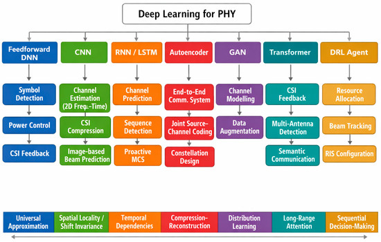
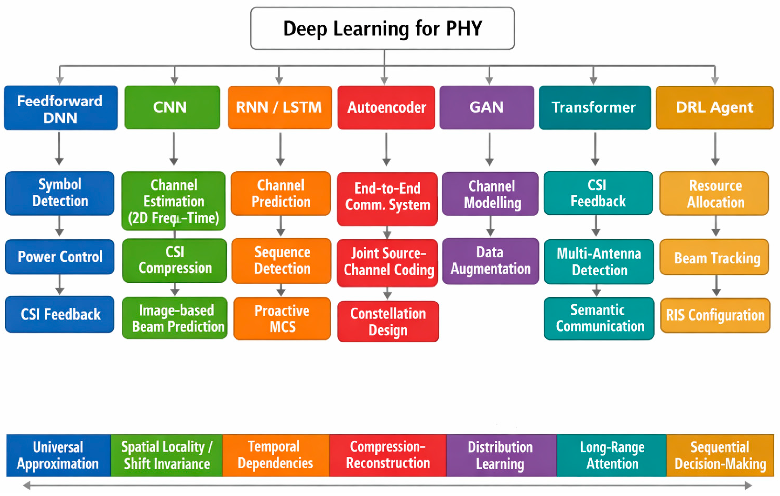
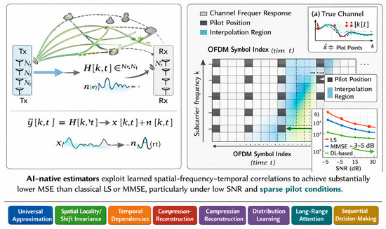
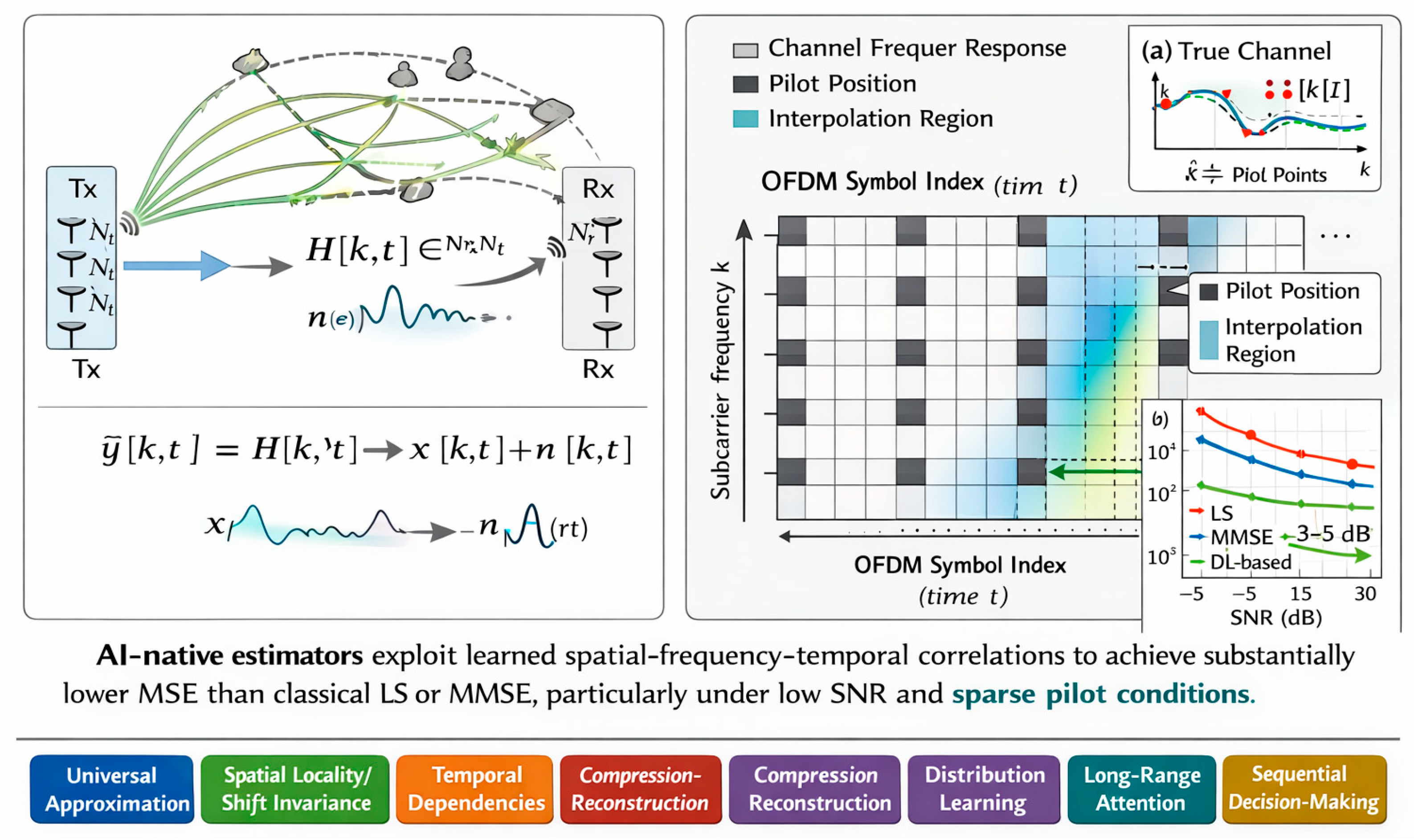
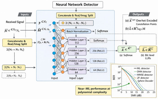
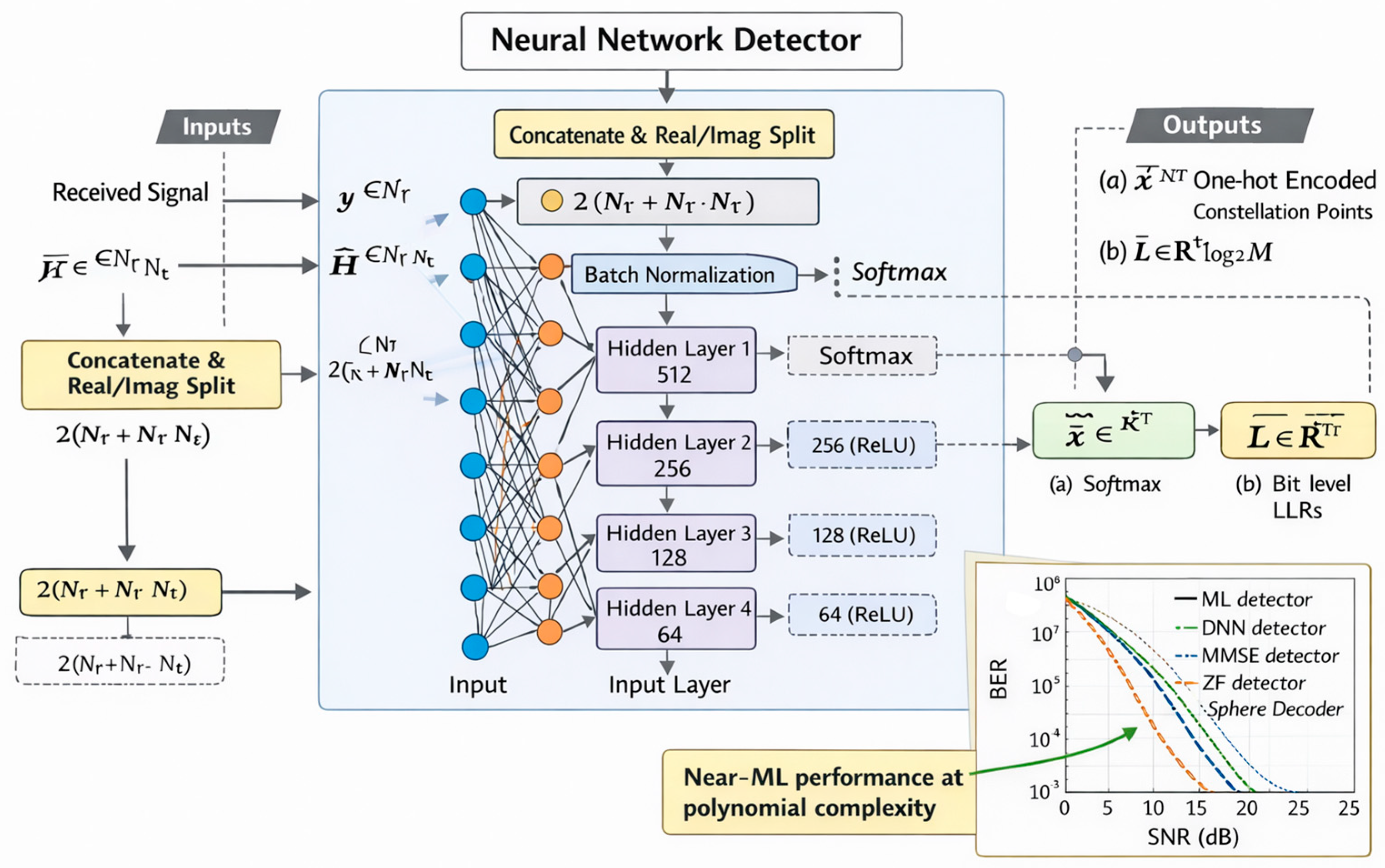
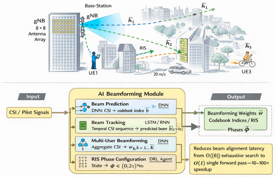
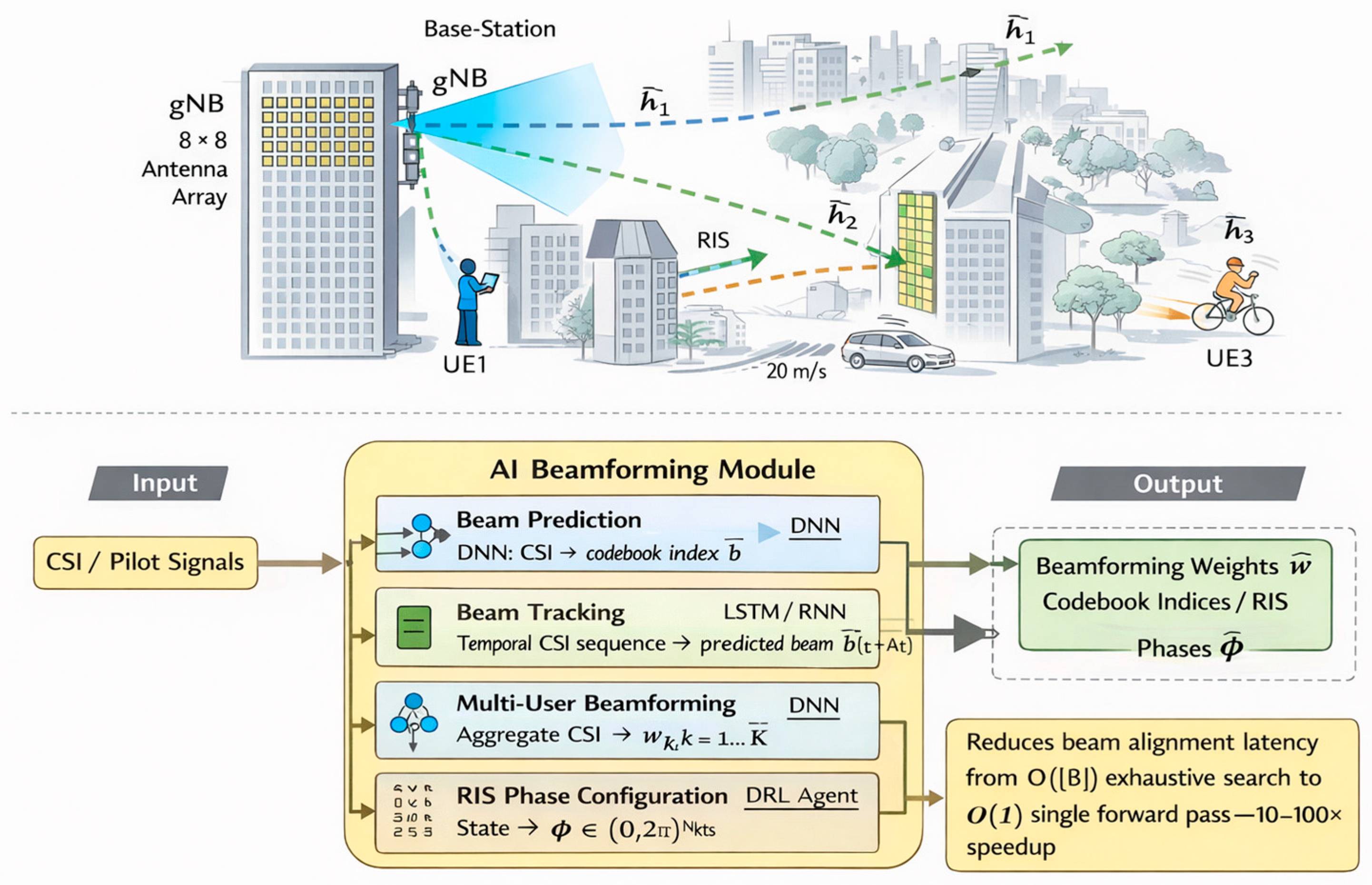
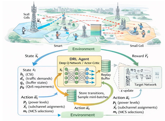
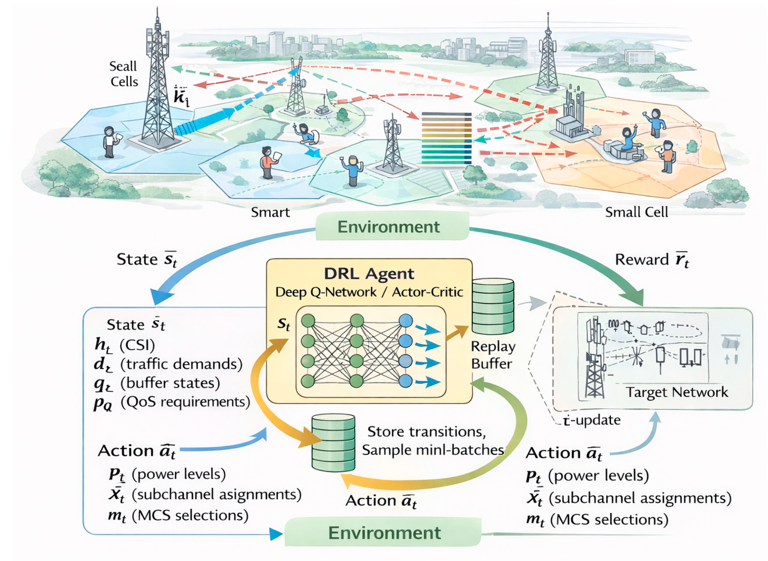
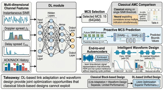
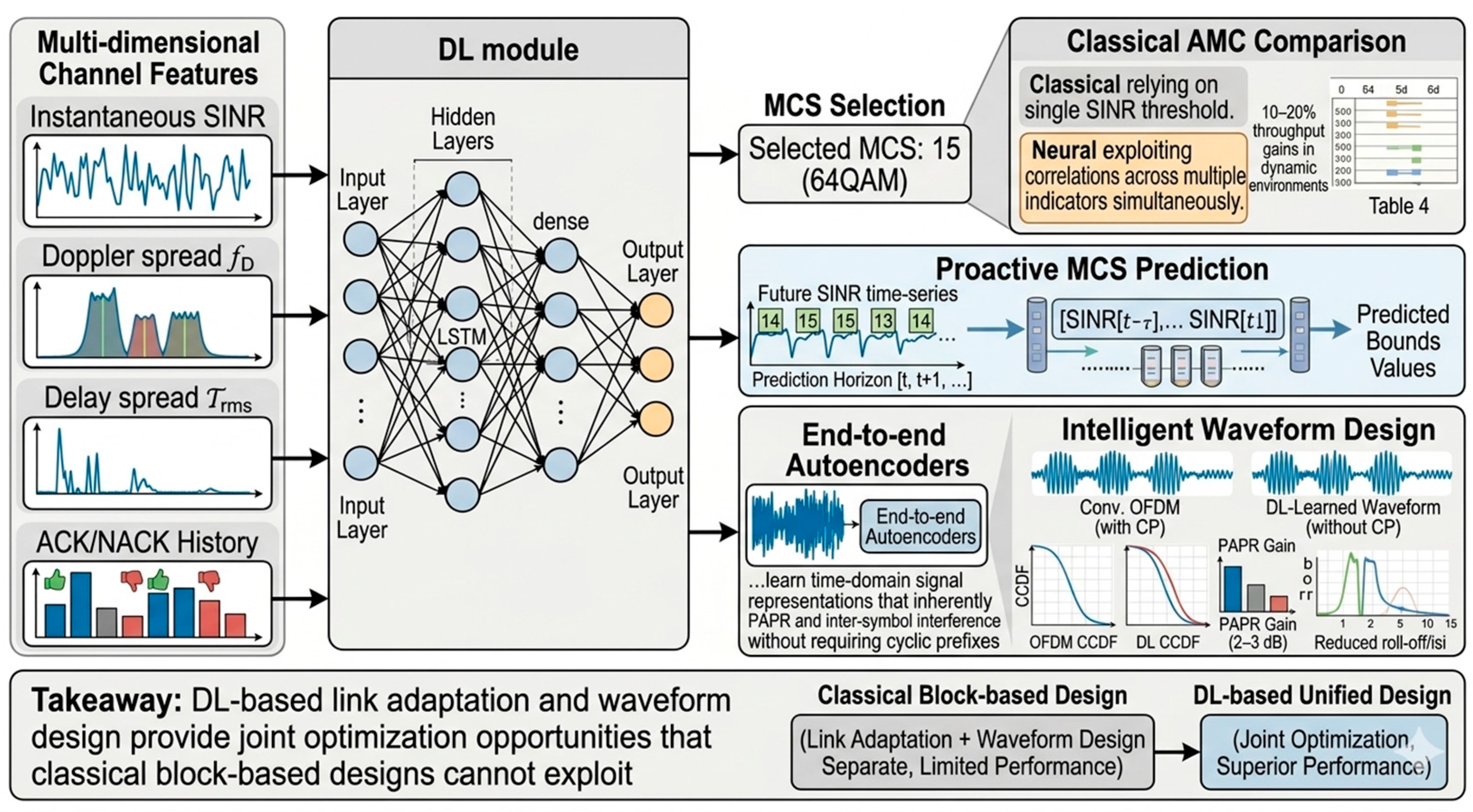
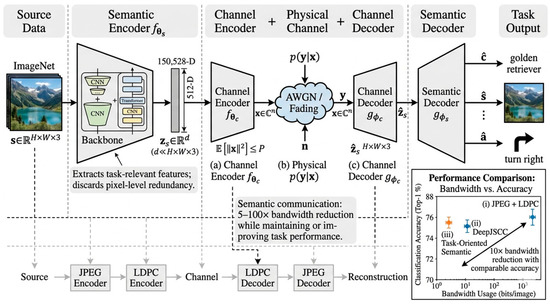
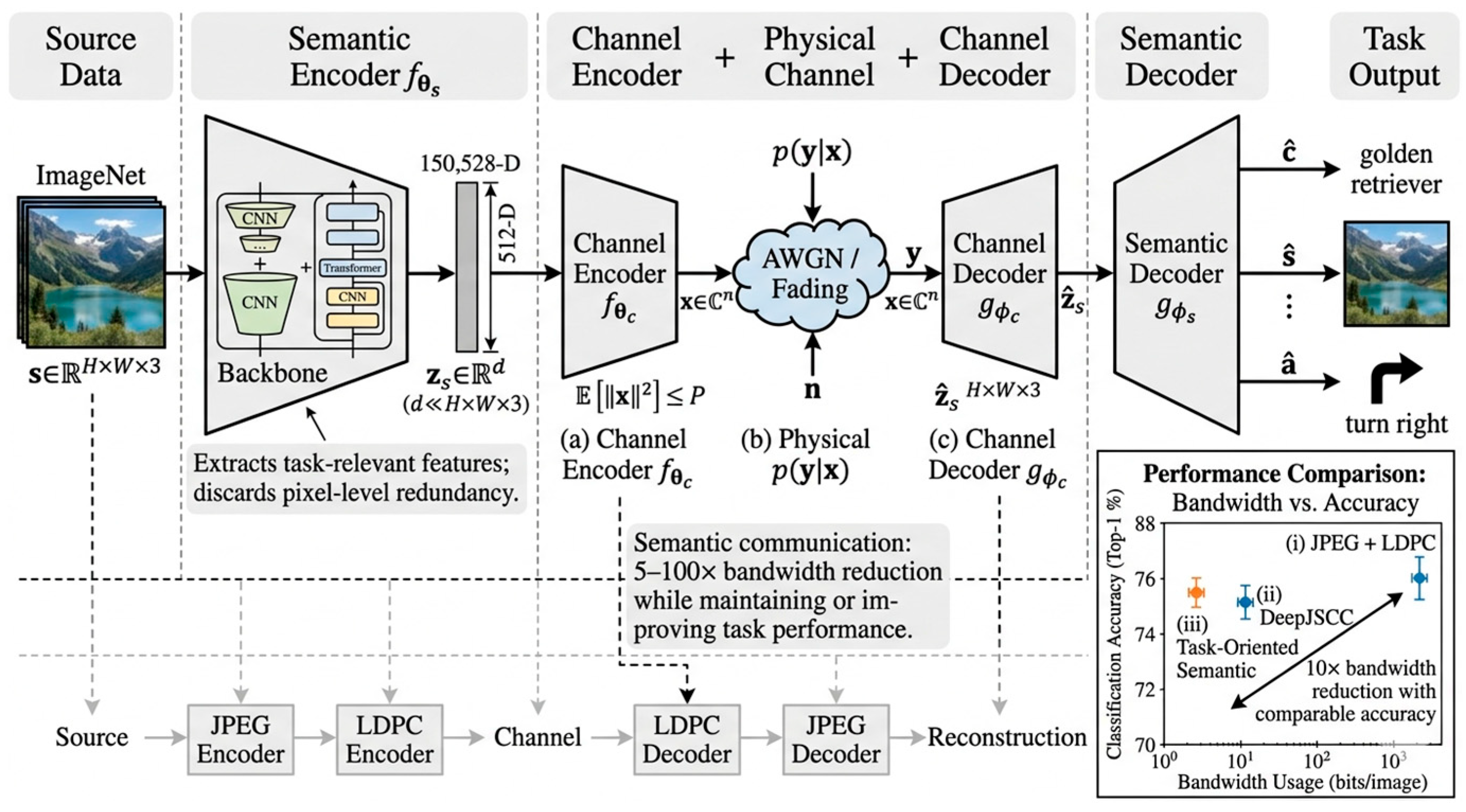

Disclaimer/Publisher’s Note: The statements, opinions and data contained in all publications are solely those of the individual author(s) and contributor(s) and not of MDPI and/or the editor(s). MDPI and/or the editor(s) disclaim responsibility for any injury to people or property resulting from any ideas, methods, instructions or products referred to in the content. |
© 2026 by the authors. Licensee MDPI, Basel, Switzerland. This article is an open access article distributed under the terms and conditions of the Creative Commons Attribution (CC BY) license.