Omni-Flex GraphFormer: Parallel Fusion of Local Graph Aggregation and Global Attention Across Image Resolutions

Abstract

Graph neural networks (GNNs) capture local image structure with few parameters, whereas Vision Transformers (ViTs) model global context at a higher computational cost. We propose the Omni-Flex GraphFormer, which applies a graph branch (OMNIVIG: max-relative aggregation over a fixed $3\times 3$ pixel neighbourhood) and a Transformer branch (FLEXIVIT: global multi-head self-attention) in parallel and sums their outputs. Because each baseline is the hybrid with one branch removed, comparing the three models on eight datasets from $8\times 8$ to $96\times 96$ pixels, under equal training budgets and over three seeds, is a controlled branch ablation. Global attention is decisive: the hybrid exceeds OMNIVIG in test macro-F1 on every dataset and in all 24 runs, by $3.7$ to $15.1$ points (Wilcoxon test, $p=0.0078$). Against FLEXIVIT, the hybrid has the best mean F1 on six datasets and a 40–$62\%$ smaller seed-to-seed spread on CIFAR-10 and CIFAR-100, but the difference is not significant ($p=0.38$). The graph branch adds only $0.5$–$3.1\%$ to the number of multiply–accumulate operations, and under warmed-up timing, both models run at the same speed, whereas unwarmed timing overstates latency by up to $15\times$. Under Gaussian noise, the summed hybrid degrades like the graph branch, which motivates gated or attention-guiding fusion.

1. Introduction

Vision Transformers (ViTs) [1] moved image recognition from convolutions to attention over patch tokens, while graph-based models such as Vision GNN [2] treat an image as an irregular graph rather than a grid. Recent Vision GNNs reduce the cost of building this graph, for example by replacing the k-nearest-neighbour search with fixed or axial connection patterns [3,4,5], and some combine graph layers with global attention [6]. Each approach is weak where the other is strong. We implement two baselines, OMNIVIG (a graph model extending Vision GNN [2]) and FLEXIVIT (a Transformer extending FlexiViT [7]), and combine them in a hybrid, the Omni-Flex GraphFormer.

1.1. Motivation

We are motivated by deployment on small devices. Self-attention costs $\mathcal{O}\left(N^2\right)$ in the number of tokens N, which is a problem on microcontrollers. Graph models such as Vision GNN [2] are cheaper, but each layer sees only a local neighbourhood, which limits reasoning about the whole scene. We combine the cheap local features of a graph with attention for global context.

1.2. Research Gap

Most hybrids of graph models and Transformers stack the two in sequence, so that one module feeds the next. Fewer works run a graph branch and an attention branch side by side on the same input and compare the fused model against each branch alone, across a wide range of image resolutions and under input noise. We study this simple parallel design to measure what each branch contributes.

1.3. Overview of the Three Models

We evaluate three models: a graph baseline, a Transformer baseline, and a hybrid of the two.

• OMNIVIG (graph baseline): Our implementation of a graph vision model built on Vision GNN [2]. Each pixel of the feature map is a node connected to its 8 spatial neighbours, and the layer applies max-relative graph convolution over this fixed neighbourhood. It captures outlines and edges well, but each layer moves information only a few hops, so relating distant parts of the image takes many layers.
• FLEXIVIT (Transformer baseline): Our implementation of a Transformer extending FlexiViT [7]. Multi-head self-attention (MHA) relates every token (one per feature-map position) to every other token. It has no built-in preference for informative regions over background; its cost grows as $\mathcal{O}\left(N^2\right)$, and, without a positional embedding, it has no explicit notion of local structure.
• HYBRID (Omni-Flex): Two branches run in parallel on the same input, and their outputs are summed. The graph branch does not modify the attention scores; the two branches are combined only at their outputs (late fusion). The cost of the hybrid is therefore the cost of the Transformer branch plus the small cost of the graph branch. We test the hypothesis that the two branches supply complementary local and global features, and measure what each branch contributes.

1.4. Summary of Results

Across eight benchmarks whose pixel counts span a factor of 144, under equal per-dataset training budgets and over three seeds, the results are as follows.

• Global attention is the decisive component. The hybrid exceeds the graph branch alone (OMNIVIG) in test macro-F1 on every dataset and in all 24 seed-level runs, by $3.7$ to $15.1$ points (Wilcoxon $p=0.0078$, the smallest value attainable with eight datasets).
• Adding the graph branch to attention costs almost nothing. The hybrid has the best mean test F1 on six of the eight datasets and is ahead of FLEXIVIT in every seed on CIFAR-10, Fashion-MNIST and SVHN. On CIFAR-10 and CIFAR-100, the seed-to-seed standard deviation of its test F1 is 40–$62\%$ smaller than FLEXIVIT’s. Over the eight datasets, however, the difference from FLEXIVIT is not significant ($p=0.38$), and FLEXIVIT is better on Micro-Digits.
• Cost. The hybrid has 4–$6\%$ more parameters and $0.5$–$3.1\%$ more MACs than FLEXIVIT; under a warmed-up protocol, their latencies are equal within measurement noise. A single unwarmed timing pass overstates per-image latency by up to $15\times$ on the smallest test set.
• Noise. On Micro-Digits, the summed hybrid degrades under Gaussian noise like OMNIVIG, whereas FLEXIVIT degrades most slowly ($34.6\%$ against $29.9\%$ for the hybrid at $\sigma =0.35$).

In short, a plain sum of a local graph branch and a global attention branch matches attention at almost no extra cost and is more stable on some datasets, but it does not by itself add accuracy or robustness. This identifies the fusion rule, rather than the choice of branches, as the point to improve.

1.5. List of Contributions

The core contributions of this work are as follows:

1.

Architecture: A hybrid that runs a graph branch, using Max-Relative graph convolution (MR-Conv), over a fixed $3\times 3$ neighbourhood, alongside a Transformer branch, with the two outputs summed.

2.

Multi-resolution branch ablation: Evaluation on eight datasets, from $8\times 8$ digits to $96\times 96$ natural images, in which each baseline is the hybrid with one branch removed, with three training seeds per configuration. It shows that global attention carries most of the accuracy of the hybrid, and that the graph branch can be added at almost no cost.

3.

Latency and cost: Inference latency, parameter count and training time for all three models on every dataset, together with token counts and analytical multiply–accumulate (MAC) counts. Comparing a warmed-up, repeated protocol with a single unwarmed call quantifies how much one-time overhead distorts per-image latency on small test sets.

4.

Noise study: Test accuracy of all three models under Gaussian input noise with $\sigma$ from $0.10$ to $0.35$, over three training seeds and five noise draws.

5.

Statistical analysis: Wilcoxon signed-rank tests of the test-F1 differences across the eight datasets and across the 24 seed-level runs.

1.6. Structure of the Paper

Section 2 reviews related work. Section 3 describes the two baselines and their limitations on a worked $8\times 8$ example. Section 4 describes the Omni-Flex GraphFormer. Section 5 covers the experiments, the significance test, the noise study, saliency maps and discussion, including the limitations of the study. Section 6 concludes.

2. Related Work

This section covers graph neural networks for vision, Vision Transformers, hybrids of the two, and work on efficiency benchmarking.

2.1. Graph Neural Networks in Vision (ViG)

Convolutional networks exploit local translation invariance on a regular grid. Graph neural networks (GNNs) instead represent an image as a set of nodes and edges, so the receptive field can adapt to the content. Early spectral approaches [8,9] led to graph convolutional networks (GCNs) [10], which give a simple layer-wise propagation rule. GraphSAGE [11] added neighbour sampling so that GNNs scale to large graphs, and graph attention networks (GAT) [12] and GATv2 [13] learn a weight for each neighbour.

Vision GNN (ViG) [2] applied this idea to images by building a k-nearest-neighbour (k-NN) graph over patches. Related graph models for point clouds include Point-GNN [14] and DGCNN [15], which uses EdgeConv and rebuilds its graph dynamically. Hierarchical pooling methods such as DiffPool [16], SAGPool [17] and gPool [18] coarsen the graph between layers. Cluster-GCN [19] improves training efficiency, and the Graph Isomorphism Network (GIN) [20] characterises how well message-passing GNNs can distinguish graphs.

Several recent works reduce the cost of graph construction. MobileViG [3] replaces the k-NN search with a fixed graph in which each pixel is linked to every K-th pixel of its row and column, and keeps MR-Conv for aggregation. MobileViGv2 [4] makes this graph sparser and adds conditional positional encodings. GreedyViG [5] builds a dynamic axial graph that considers fewer connections than k-NN. AdaptViG [6] combines a static axial scaffold with a content-aware gate and places a global attention block in its final stage; graph processing and attention are applied in sequence, whereas the hybrid studied here applies them in parallel and sums their outputs.

OMNIVIG follows this line with a simplification: instead of a k-NN graph built in feature space, it uses the fixed 8-neighbour pixel grid, over which the max-relative aggregation emphasises local gradients. Deep GNNs suffer from over-smoothing [21]: node features become similar as layers accumulate. JK-Net [22] and DeepGCNs [23,24] address it with skip and dilated connections, and PairNorm [25] and DropEdge [26] with normalisation and edge dropping. Graph Transformer variants [27,28] add attention over the graph, yet modelling long-range dependencies remains difficult for GNNs. This motivates adding a global attention branch.

2.2. Vision Transformers and Global Attention

The Vision Transformer (ViT) [1] showed that self-attention over a sequence of image patches can match or exceed convolutional networks when trained at scale. Multi-head self-attention (MHA) lets every patch attend to every other patch, which captures long-range dependencies. The standard ViT-Base has no built-in spatial prior, and its attention cost is $O\left(N^2\right)$ in the number of tokens.

DeiT [29] reduced the data requirements of ViT through distillation, and CaiT [30] trains deeper Transformers with LayerScale and class-attention layers. To lower the attention cost, Swin Transformer [31] and Swin-v2 [32] restrict attention to shifted windows, while the Pyramid Vision Transformer (PVT) [33] and PVTv2 [34] progressively shrink the spatial resolution. T2T-ViT [35] models local structure by merging neighbouring tokens, and Transformer-in-Transformer (TNT) [36] nests a finer attention block inside each patch.

FlexiViT [7] trains one model that works with several patch sizes, so the token count can be chosen at inference time. ScalableViT [37] lowers the cost of attention on large images, and CrossViT [38] combines tokens from patches of two sizes. XCiT [39] applies attention across feature channels rather than tokens, which makes the cost linear in the number of tokens, and DINOv2 [40] learns general-purpose features by self-supervised pre-training. MobileViT [41], MobileViTv2 [42] and FastViT [43] target mobile devices.

Another line of work reduces the number of tokens. SparseViT [44] exploits activation sparsity, and TokenLearner [45] learns a small set of tokens adaptively. UniFormer [46] and MViTv2 [47] add convolutions or pooling to bring in local priors. FlexiViT [7] lets the token count vary through the patch size. Pure attention models still have no explicit notion of image structure, which is what our graph branch is meant to supply.

2.3. Hybrid Architectures and Functional Fusion

Several hybrids add local structure to Transformers through convolutions. ConViT [48] initialises attention heads to behave like convolutions, and CMT [49] and CvT [50] use convolutional projections and blocks. LeViT [51] and BoTNet [52] combine convolutional and attention stages for faster inference. CoAtNet [53] combines depthwise convolution with self-attention, and LocalViT [54] inserts depthwise convolution into the feed-forward layers.

Other hybrids combine graphs and Transformers. Graph-Transformer [27], GTN [28] and Graphormer [55] apply attention to graph data, and Global Filter Networks [56] mix tokens globally in the frequency domain. GraphTrans [57], TokenGT [58] and GPS [59] run graph and attention modules in sequence or in alternation, so that one module feeds the next. MobileViT [41], MobileViTv2 [42] and EdgeViT [60] are hybrids designed for limited hardware. FastViT [43], UniFormer [46] and MViTv2 [47] combine multi-scale features with efficient attention.

SparseViT [44] and FlexiViT [7] reduce cost by adapting sparsity or patch size. Our Omni-Flex GraphFormer differs from the sequential designs above, such as GPS [59] and NodeFormer [61], in that its two branches run in parallel on the same input and are fused only at their outputs. This design does not reduce the cost of attention, which recent surveys [62,63] treat as a central issue; it aims to add local structure at a small extra cost.

2.4. Efficiency and Benchmarking

Evaluation now goes beyond top-1 accuracy. Latency, parameter count and throughput are reported alongside it, and no single one of them measures cost adequately [64]. The Pareto frontier is a common way to compare models on this trade-off [65,66]. Energy use and carbon footprint are also increasingly reported.

Hardware-aware neural architecture search [67,68] optimises models for measured latency on a target device, and energy-aware design [69] accounts for memory access and energy. Benchmark suites such as MLPerf [70] and TinyML benchmarks [71] show that theoretical complexity often differs from measured wall-clock time. The Green AI movement [72] encourages reporting energy or carbon cost [73,74].

Most comparisons are made at a single resolution. We instead evaluate on eight datasets whose pixel counts span a factor of 144. We compare models with the Wilcoxon signed-rank test [75,76], a non-parametric test recommended for comparing classifiers over several datasets [77,78]. We report inference latency and discuss where our protocol falls short of standard benchmarking practice [79], and report parameter counts as an efficiency measure [80,81].

3. Methodological Tools

This section describes the two baselines exactly as implemented and evaluated. All three models share the same convolutional stem and classification head and differ only in the single layer placed between them (Section 4).

3.1. Shared Notation and Stem

An input image $I\in {\mathbb{R}}^{H\times W\times c_{in}}$ is passed through a convolutional stem (a $k\times k$ convolution with C output channels, ReLU activation and “same” padding), which gives a feature map $X\in {\mathbb{R}}^{H^{\prime }\times W^{\prime }\times C}$. For every dataset except STL-10, the stem uses $k=3$ and stride 1, so $H^{\prime }=H$ and $W^{\prime }=W$. For STL-10, it uses $k=7$ and stride 4, which reduces $96\times 96$ inputs to $24\times 24$. Each spatial position i of X is one node of the graph branch and one token of the Transformer branch, and $h_i\in {\mathbb{R}}^C$ denotes its feature vector. The number of nodes (tokens) is $N=H^{\prime }{W}^{\prime }$. After the evaluated layer, global average pooling and a dense softmax layer produce the class probabilities.

3.2. OMNIVIG: Graph-Based Vision Baseline

3.2.1. Principle of the Graph Layer

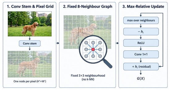
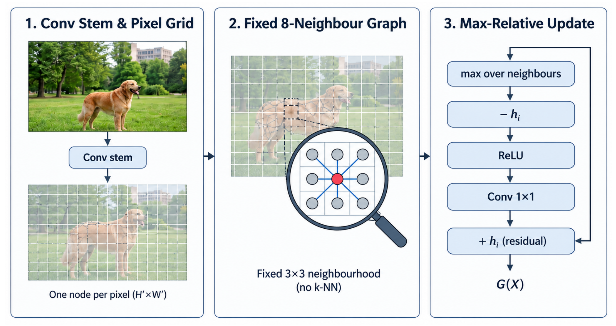
OMNIVIG builds on the max-relative graph convolution (MR-Conv) of Vision GNN [2], with one simplification. Vision GNN links each node to its k nearest neighbours in feature space. OMNIVIG instead uses a fixed spatial graph: each node is linked to its 8 neighbours in the pixel grid ($k=8$), so its neighbourhood is the $3\times 3$ window $\mathcal{W}\left(i\right)$ centred on i, which includes i itself. No distances are computed, and the cost is linear in N. The price is that, unlike Vision GNN, nodes that look similar but are far apart are never linked. Figure 1 shows the layer.

Figure 1. Schematic depiction of the OMNIVIG layer. (1) The convolutional stem gives one node per feature-map position ($H^{\prime }\times W^{\prime }$). (2) Each node is linked to its 8 neighbours in a fixed $3\times 3$ window; no k-NN search is performed. (3) Max-relative update: maximum over the neighbourhood, subtraction of $h_i$, ReLU, $1\times 1$ convolution and residual connection, giving $G\left(X\right)$ (Equations (1)–(3)).

The layer computes, channel by channel,

$$\begin{array}{c}{m}_i=\underset{j\in \mathcal{W}\left(i\right)}{\max }{h}_j,\end{array}$$

(1)

$$\begin{array}{c}{\mathrm{\Delta }}_i=\mathrm{ReLU}\left(m_i-h_i\right)=\underset{j\in \mathcal{W}\left(i\right)}{\max }\left(h_j-h_i\right),\end{array}$$

(2)

$$\begin{array}{c}G{\left(X\right)}_i=h_i+{\mathbf{W}}_g{\mathrm{\Delta }}_i+{\mathbf{b}}_g,\end{array}$$

(3)

where ${\mathbf{W}}_g\in {\mathbb{R}}^{C\times C}$ and ${\mathbf{b}}_g\in {\mathbb{R}}^C$ are the weights of a $1\times 1$ convolution. The relative differences $h_j-h_i$ cancel a uniform brightness shift and respond strongly at boundaries, and the maximum keeps the strongest local contrast, whereas averaging would blur it. Because the window contains node i itself, $m_i\ge h_i$ and ${\mathrm{\Delta }}_i$ is never negative; the ReLU is a safeguard rather than a correction. The residual term $h_i$ keeps the original features. Figure 1 illustrates the layer.

3.2.2. Graph Layer on an $8\times 8$ Example

The following example illustrates the operations of each layer; it is not evidence of performance. We use the following image $I\in {\mathbb{R}}^{8\times 8}$, which contains an intensity gradient, and treat each pixel value as a one-channel feature.

$$I=\left[\begin{array}{cccccccc}12& 18& 22& 25& 28& 30& 35& 40\\ 15& 20& 24& 29& 33& 38& 42& 45\\ 18& 23& 27& 35& 40& 48& 52& 58\\ 20& 26& 32& 44& 60& 72& 80& 88\\ 22& 28& 36& 58& 90& 120& 135& 142\\ 24& 30& 42& 70& 118& 160& 180& 190\\ 26& 34& 48& 82& 140& 185& 210& 225\\ 28& 38& 55& 95& 155& 205& 235& \mathbf{250}\end{array}\right]$$

(4)

• Local contrast: The window of pixel $(7,7)$, value 210, contains the value 250 at $(8,8)$, so $\mathrm{\Delta }=250-210=40$. Pixel $(8,8)$ is the largest value in its own window, so $\mathrm{\Delta }=0$. The term $\mathrm{\Delta }$ therefore marks pixels that are darker than a neighbour, i.e., edges, and is exactly zero on a local peak.
• Limited reach: One layer sees only a $3\times 3$ window. Information from $(1,1)$ would reach $(8,8)$ only after 7 stacked layers. The evaluated models use a single layer, so on its own the graph branch has no long-range interaction before the final global average pooling.

3.3. FLEXIVIT: Transformer-Based Baseline

3.3.1. Principle of the Attention Layer

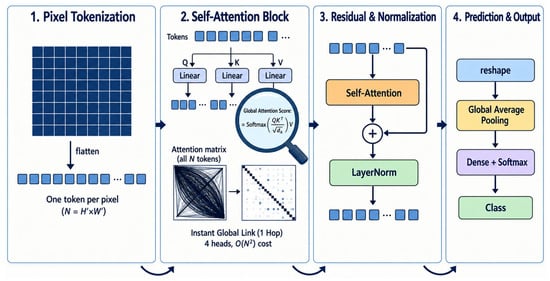
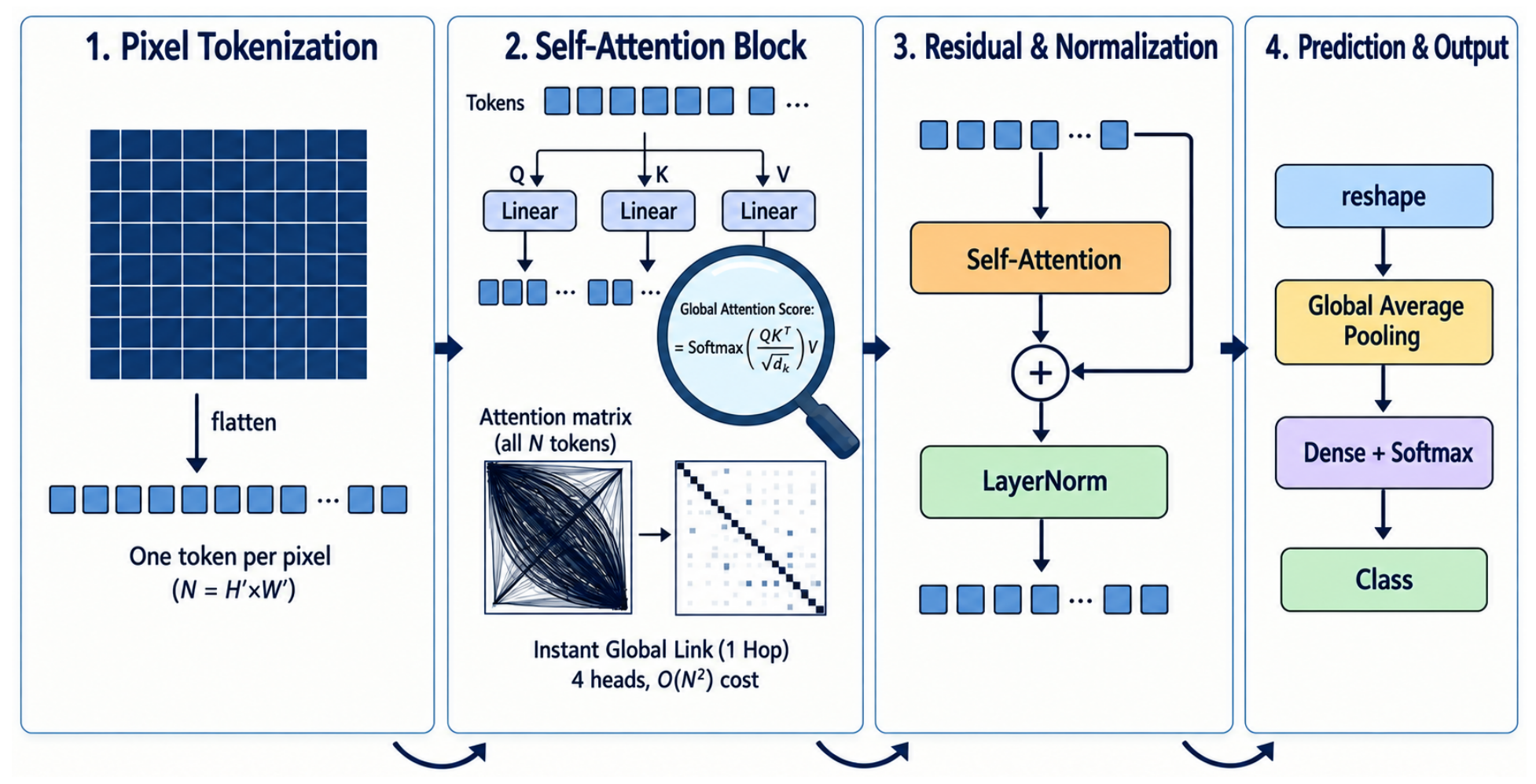
FLEXIVIT is a single Transformer layer whose name refers to the FlexiViT design that motivated it [7]. In the evaluated models, the tokenisation is fixed: there is one token per position of X, so the token count is $N=H^{\prime }{W}^{\prime }$. FlexiViT’s flexible patch size and saliency-driven adaptive patching are not part of the evaluated models and are left to future work. No positional embedding is added; spatial information enters only through the convolutional stem. Figure 2 shows the layer.

Figure 2. Schematic depiction of the FLEXIVIT layer. (1) The feature map is flattened into one token per position ($N=H^{\prime }{W}^{\prime }$); there is no adaptive patching. (2) Multi-head self-attention with 4 heads links every token to every other token in one step, at $\mathcal{O}\left(N^2\right)$ cost. (3) Residual connection followed by layer normalisation, giving $T\left(X\right)$. (4) Reshape, global average pooling and dense softmax classifier.

The feature map is reshaped into a token matrix $Z\in {\mathbb{R}}^{N\times C}$. Each of the 4 heads computes the scaled dot-product attention of Vaswani et al. [82],

$${\mathrm{Attn}}_h\left(Z\right)=\mathrm{Softmax}\left({\displaystyle \frac{\left(Z{\mathbf{W}}_Q^h\right){\left(Z{\mathbf{W}}_K^h\right)}^T}{\sqrt{d_k}}}\right)Z{\mathbf{W}}_V^h,d_k=C,$$

(5)

the heads are concatenated and projected back to C channels to give $\mathrm{MHA}\left(Z\right)$, and the layer output is

$$T\left(X\right)=\mathrm{LayerNorm}\left(Z+\mathrm{MHA}\left(Z\right)\right),$$

(6)

reshaped back to $H^{\prime }\times W^{\prime }\times C$. Figure 2 illustrates the layer.

3.3.2. Attention Layer on an $8\times 8$ Example

• Global reach: Every token attends to every other token, so $(1,1)$ and $(8,8)$ interact in a single layer.
• Averaging: Each row of the softmax sums to one, so the attention output at a token is a weighted average of the value vectors. A weighted average cannot exceed the largest value and tends to smooth peaks. For example, with identity projections and uniform attention over the 64 pixels, every token would receive the image mean, $72.4$, whereas pixel $(8,8)$ has the value 250. The residual connection keeps the original value, but attention itself supplies no explicit local-difference signal such as $\mathrm{\Delta }$.
• Cost: The 64 tokens of the example give ${64}^2=4096$ attention scores per head; a $32\times 32$ feature map gives 1,048,576.

4. The Omni-Flex GraphFormer

4.1. Parallel Fusion

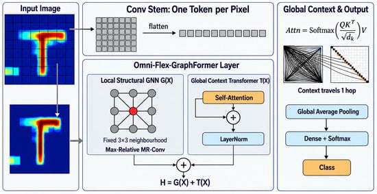
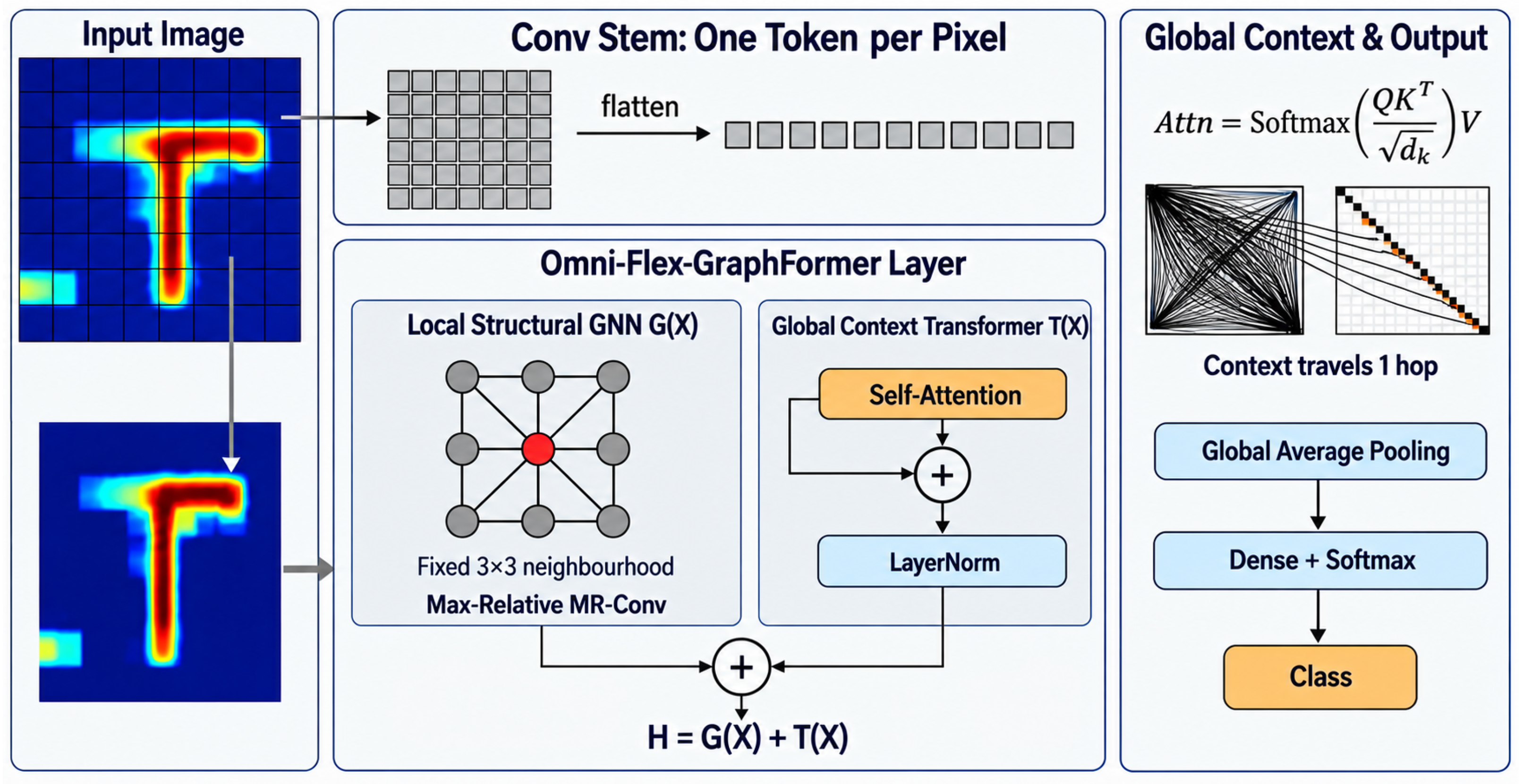
The Omni-Flex GraphFormer applies both layers to the same feature map X and sums their outputs:

$$H=\underset{\mathrm{local}\mathrm{detail}}{\underbrace{G\left(X\right)}}+\underset{\mathrm{global}\mathrm{context}}{\underbrace{T\left(X\right)}}.$$

(7)

The sum is unweighted; there are no learnable fusion weights. The graph branch does not modify the attention scores: the two branches interact only at their outputs (late fusion). Global average pooling and a dense softmax layer follow, as in the baselines. Figure 3 shows the design.

Figure 3. Schematic depiction of the Omni-Flex GraphFormer. The convolutional stem gives one token per position. The OMNIVIG branch $G\left(X\right)$ (fixed $3\times 3$ neighbourhood, MR-Conv) and the FLEXIVIT branch $T\left(X\right)$ (self-attention, residual connection, layer normalisation) are applied in parallel to the same feature map, and their outputs are summed without weights, $H=G\left(X\right)+T\left(X\right)$. Global average pooling and a dense softmax layer follow. The input image is illustrative.

4.2. The Baselines as a Branch Ablation

The three models differ only in the evaluated layer: OMNIVIG uses G, FLEXIVIT uses T, and the hybrid uses $G+T$. Each baseline is therefore the hybrid with one branch removed, and the comparison in Section 5 is a branch ablation. The hybrid has exactly $C^2+C$ more parameters than FLEXIVIT, those of the $1\times 1$ convolution ${\mathbf{W}}_g$ (e.g., 4160 for $C=64$).

4.3. Computational Cost

Counting multiply–accumulate operations (MACs) per image and excluding the stem and head, which are identical in all three models, the graph branch costs $N{C}^2$ MACs for the $1\times 1$ convolution; the $3\times 3$ maximum costs only comparisons. With 4 heads of key dimension C, the Transformer branch costs $16N{C}^2$ MACs for the query, key, value and output projections and $8N^{2}C$ MACs for the attention scores and the weighted sum of values. Hence

$${\mathrm{MAC}}_G=N{C}^2,{\mathrm{MAC}}_T=16N{C}^2+8N^{2}C,{\mathrm{MAC}}_{\mathrm{hybrid}}={\mathrm{MAC}}_G+{\mathrm{MAC}}_T.$$

(8)

The graph branch is linear in N, but the hybrid remains quadratic. Table 1 gives the values for each dataset: the graph branch adds between $0.5\%$ and $3.1\%$ to the cost of the Transformer branch, so the hybrid cannot be meaningfully faster than FLEXIVIT. Although the two branches are independent and could in principle run concurrently, our implementation does not exploit this, and we make no claim of a speed-up.

Table 1. Token count, channel width and analytical MACs per image of the graph branch (G) and the Transformer branch (T). Stem and head are excluded because they are identical in all three models.

Dataset	Tokens N	Width C	${\mathbf{MAC}}_{\mathit{G}}$ (M)	${\mathbf{MAC}}_{\mathit{T}}$ (M)	${\mathbf{MAC}}_{\mathit{G}}$/${\mathbf{MAC}}_{\mathit{T}}$
Micro-Digits ($8\times 8$)	64	32	0.07	2.10	3.1%
USPS ($16\times 16$)	256	32	0.26	20.97	1.3%
MNIST ($28\times 28$)	784	32	0.80	170.20	0.5%
Fashion-MNIST ($28\times 28$)	784	64	3.21	366.08	0.9%
CIFAR-10 ($32\times 32$)	1024	64	4.19	603.98	0.7%
SVHN ($32\times 32$)	1024	64	4.19	603.98	0.7%
CIFAR-100 ($32\times 32$)	1024	128	16.78	1342.18	1.3%
STL-10 ($96\times 96$, stride-4 stem)	576	32	0.59	94.37	0.6%

4.4. Comparison on the $8\times 8$ Example

On the $8\times 8$ example, the hybrid output at pixel $(7,7)$ contains both the edge signal ${\mathbf{W}}_g\mathrm{\Delta }$ with $\mathrm{\Delta }=40$ from the graph branch and an attention output that depends on all 64 pixels. Table 2 summarises the properties of the three layers.

Table 2. Properties of the three evaluated layers.

Property	OMNIVIG	FLEXIVIT	Omni-Flex (Hybrid)
Reach of one layer	$3\times 3$ window	all N tokens	all N tokens
Explicit local contrast $\mathrm{\Delta }$	yes	no	yes
Cost as a function of N	linear	quadratic	quadratic

5. Experimentation

5.1. Development Environment and Architectural Framework

All three models were implemented in the same framework, so that differences in the results come from the architectures rather than from the software environment. This section describes the software stack, the three models, the training setup and the measurement protocol.

5.1.1. Coding Environment and Software Stack

• Primary Framework: TensorFlow 2.21 with keras.ops.
• Environment: Python 3.11+ with NumPy and Pandas for data handling and logging.
• Hardware: All runs were performed on a Google Colab instance with an NVIDIA T4 GPU (NVIDIA Corporation, Santa Clara, CA, USA), in FP32.
• Evaluation Metrics: Scikit-learn 1.6.1 for macro-F1 and classification reports.
• Inference Benchmarking: Python’s time.perf_counter(); the protocol is described in Section 5.4.

5.1.2. Architectural Profiles

Table 3 summarises the three models; their layers are defined in Section 3 and Section 4.

Table 3. Structural and coding characteristics of the evaluated models.

Feature	OMNIVIG	FLEXIVIT	HYBRID
Primary Logic	Max-relative aggregation	Global self-attention	Sum of both branches
Neighbourhood	Fixed $3\times 3$ grid ($k=8$)	All N tokens	Both
Complexity	Linear $\mathcal{O}\left(N{C}^2\right)$	Quadratic $\mathcal{O}(N^{2}C+N{C}^2)$	Quadratic $\mathcal{O}(N^{2}C+N{C}^2)$
Positional Information	Implicit (grid)	Stem convolution only	Both

OMNIVIG Configuration

The OMNIVIG layer computes $\mathrm{ReLU}({\max \_\mathrm{pool}}_{3\times 3}\left(x\right)-x)$, applies a $1\times 1$ convolution and adds the result to x (Equations (1)–(3)). This keeps the model small.

FLEXIVIT Configuration

The FLEXIVIT layer uses multi-head self-attention (MHA) with four heads over one token per feature-map position, so any two positions in the image can interact directly, followed by a residual connection and layer normalisation.

HYBRID (Omni-Flex) Configuration

In the code, the input x passes through both the OMNIVIG and FLEXIVIT branches, and their outputs are summed ($x_{gnn}+x_{vit}$). The GNN output does not enter the attention computation.

5.1.3. Training Setup

All models were trained from scratch with the Adam optimiser (default learning rate ${10}^{-3}$) and sparse categorical cross-entropy. Inputs were scaled to $[0,1]$. No data augmentation, learning-rate schedule or early stopping was used; on CIFAR-100 only, a dropout layer (rate $0.3$) precedes the classifier in all three models. Within each dataset, the three models share the same stem, width, batch size and number of epochs (Table 4), so the comparison is made under an equal training budget. The budgets differ between datasets, and several are short, so absolute accuracies are well below published state-of-the-art values; the study compares the three layers under equal conditions and does not aim at state-of-the-art accuracy.

Table 4. Training configuration per dataset; each configuration was run with three seeds. Train/test splits are the standard ones (USPS: 7291/2007 images; SVHN: 73,257/26,032; STL-10: 5000/8000 labelled images), except Micro-Digits (random 80/20 split, 360 test images).

Dataset	Stem	Width C	Tokens N	Batch	Epochs	Test Images
Micro-Digits	$3\times 3$, stride 1	32	64	32	30	360
USPS	$3\times 3$, stride 1	32	256	64	50	2007
MNIST	$3\times 3$, stride 1	32	784	64	10	10,000
Fashion-MNIST	$3\times 3$, stride 1	64	784	64	15	10,000
SVHN	$3\times 3$, stride 1	64	1024	128	15	26,032
CIFAR-10	$3\times 3$, stride 1	64	1024	128	30	10,000
CIFAR-100	$3\times 3$, stride 1	128	1024	64	15	10,000
STL-10	$7\times 7$, stride 4	32	576	64	30	8000

Every configuration was trained with three random seeds (0, 1, 2), which set the weight initialisation and the order of the training data, giving $8\times 3\times 3=72$ runs.

5.2. Dataset Descriptions

We use eight datasets, from $8\times 8$ digits to $96\times 96$ natural images (Table 5).

Table 5. Characteristics of the datasets used in this study.

Dataset	Resolution	Channels	Classes	Samples	Domain
Micro-Digits	$8\times 8$	1	10	1797	Low-res handwritten digits
USPS	$16\times 16$	1	10	9298	Handwritten digits
MNIST	$28\times 28$	1	10	70,000	Handwritten digits
Fashion-MNIST	$28\times 28$	1	10	70,000	Greyscale clothing items
SVHN	$32\times 32$	3	10	99,289	Street view house numbers
CIFAR-10	$32\times 32$	3	10	60,000	Natural objects/animals
CIFAR-100	$32\times 32$	3	100	60,000	Fine-grained objects
STL-10	$96\times 96$	3	10	13,000	High-res natural images

The selection includes:

• Handwritten Digits (Micro-Digits, USPS, MNIST): Used to test architectural efficiency and local feature extraction at varying degrees of resolution.
• Texture and Geometry (Fashion-MNIST): Focuses on greyscale texture discrimination and silhouette identification.
• Real-World Digits (SVHN): Introduces background clutter, varied lighting, and natural distortions.
• Natural Scenes (CIFAR-10/100, STL-10): Challenges the model with high-granularity classification and, in the case of STL-10, higher spatial resolutions.

5.3. Evaluation Metrics

For each model, we report test accuracy, test macro-F1, inference latency, training time and parameter count. Each configuration was trained with three random seeds (0, 1, 2), and the tables give the mean ± standard deviation over the three runs; the best mean test accuracy and test F1 of each dataset are in bold. Accuracy and macro-F1 are both computed on the held-out test set and are given in per cent. Training time is the sum of the epoch times, excluding checkpoint saving. Latency is given per test image under two protocols, described in Section 5.4: the warm protocol (warm-up pass followed by 10 timed passes; mean ± standard deviation over seeds of the per-run mean), which we use for all comparisons, and the unwarmed protocol (a single pass without warm-up; mean over seeds), reported to quantify the effect of one-time overhead.

5.4. Latency Measurement Protocol

All timings were taken on the T4 GPU in FP32, with model.predict() at batch size 32 and Python’s time.perf_counter(), immediately after training. Because predict() returns host-side NumPy arrays, each measurement includes completed GPU execution and device-to-host transfer, so GPU synchronisation is implicit. Latency is reported per test image, i.e., the time of a pass over the whole test set divided by the number of test images n. Two protocols are reported.

• Warm protocol (used for all comparisons). One warm-up call on the first $\min (n,320)$ test images, then 10 timed passes over the whole test set. For each run we record the mean and standard deviation of the 10 passes; the tables give the mean over the three seeds of the per-run means, ± their standard deviation across seeds. The standard deviation over the 10 passes within a run has a median of $0.018$ ms (range $0.002$–$0.27$ ms).
• Unwarmed protocol. A single pass over the test set, timed before the warm-up call. It includes one-time costs such as building and tracing the inference graph, spread over the n test images, and shows how much these costs distort a single-call measurement.

The difference between the two protocols depends on the size of the test set, because the one-time cost is fixed. For example, on Micro-Digits ($n=360$) FLEXIVIT takes $4.13$ ms per image under the unwarmed protocol and $0.27$ ms under the warm protocol, a factor of about 15; on MNIST ($n=\mathrm{10,000}$) the same comparison gives $0.58$ and $0.40$ ms, a factor of about $1.5$. A single-call measurement therefore produces artefacts: per-image latency on Micro-Digits appears higher than on much larger images, and the hybrid can appear faster than FLEXIVIT although it performs strictly more computation. Under the warm protocol, latency follows the token count and width rather than the image size, as expected from Table 1: CIFAR-100 ($\mathrm{1,024}$ tokens, $C=128$, $1.25$ ms) is slower than STL-10 (576 tokens, $C=32$, $0.54$ ms) despite its smaller images. Python-level timing on a shared cloud GPU still has limits [79], so we treat differences of a few hundredths of a millisecond as within measurement noise and use the analytical MACs of Table 1 as the hardware-independent cost measure.

5.5. Results per Dataset

Table 6, Table 7, Table 8, Table 9, Table 10, Table 11, Table 12 and Table 13 give the results for each dataset. All tables share the column layout described in the previous subsections.

5.6. Comparative Performance Analysis on USPS Dataset

Table 6 gives the results on USPS ($16\times 16$).

Table 6. Results on USPS ($16\times 16$), 50 epochs, mean ± std over 3 seeds.

Architecture	Test Acc. (%)	Test F1 (%)	Latency, Warm (ms)	Latency, Unwarmed (ms)	Train Time (s)	Params
OMNIVIG	$80.30\pm 1.15$	$78.43\pm 1.07$	$0.102\pm 0.007$	0.669	$26.7\pm 4.0$	1706
FLEXIVIT	$89.87\pm 1.27$	$89.09\pm 1.31$	$0.149\pm 0.017$	0.960	$65.9\pm 2.7$	17,514
HYBRID	$\mathbf{89.89}\pm 0.95$	$\mathbf{89.14}\pm 1.01$	$0.134\pm 0.003$	0.864	$71.6\pm 1.3$	18,570

Bold values indicate the best mean test accuracy and test F1 on the dataset.

Table 6. Results on USPS ($16\times 16$), 50 epochs, mean ± std over 3 seeds.

Architecture	Test Acc. (%)	Test F1 (%)	Latency, Warm (ms)	Latency, Unwarmed (ms)	Train Time (s)	Params
OMNIVIG	$80.30\pm 1.15$	$78.43\pm 1.07$	$0.102\pm 0.007$	0.669	$26.7\pm 4.0$	1706
FLEXIVIT	$89.87\pm 1.27$	$89.09\pm 1.31$	$0.149\pm 0.017$	0.960	$65.9\pm 2.7$	17,514
HYBRID	$\mathbf{89.89}\pm 0.95$	$\mathbf{89.14}\pm 1.01$	$0.134\pm 0.003$	0.864	$71.6\pm 1.3$	18,570

Bold values indicate the best mean test accuracy and test F1 on the dataset.

OMNIVIG is the cheapest model: it has about $10\times$ fewer parameters than the other two, the lowest latency ($0.10$ ms) and the shortest training time, at a cost of about 10 points of test F1. FLEXIVIT and the hybrid are tied: their mean test accuracies differ by $0.02$ points and their test F1 by $0.05$ points, far less than the seed-to-seed standard deviation of about 1 point. The hybrid has the smallest spread over seeds ($\pm 0.95$ in accuracy against $\pm 1.27$ for FLEXIVIT), and its warm latency is within measurement noise of FLEXIVIT’s. On USPS, adding the graph branch therefore costs no measurable accuracy or speed.

5.7. Results on Micro-Handwritten Digits ($8\times 8$)

The $8\times 8$ digits dataset has very little spatial detail: the shape of a digit is described by a handful of pixels. Table 7 gives the results.

Table 7. Results on Micro-Handwritten Digits ($8\times 8$), 30 epochs, mean ± std over 3 seeds.

Architecture	Test Acc. (%)	Test F1 (%)	Latency, Warm (ms)	Latency, Unwarmed (ms)	Train Time (s)	Params
OMNIVIG	$86.02\pm 2.25$	$85.81\pm 2.05$	$0.263\pm 0.003$	2.282	$11.2\pm 2.0$	1706
FLEXIVIT	$\mathbf{92.04}\pm 1.37$	$\mathbf{91.76}\pm 1.42$	$0.272\pm 0.004$	4.131	$13.7\pm 2.4$	17,514
HYBRID	$90.00\pm 2.82$	$89.72\pm 2.93$	$0.316\pm 0.073$	4.802	$13.9\pm 0.4$	18,570

Bold values indicate the best mean test accuracy and test F1 on the dataset.

Table 7. Results on Micro-Handwritten Digits ($8\times 8$), 30 epochs, mean ± std over 3 seeds.

Architecture	Test Acc. (%)	Test F1 (%)	Latency, Warm (ms)	Latency, Unwarmed (ms)	Train Time (s)	Params
OMNIVIG	$86.02\pm 2.25$	$85.81\pm 2.05$	$0.263\pm 0.003$	2.282	$11.2\pm 2.0$	1706
FLEXIVIT	$\mathbf{92.04}\pm 1.37$	$\mathbf{91.76}\pm 1.42$	$0.272\pm 0.004$	4.131	$13.7\pm 2.4$	17,514
HYBRID	$90.00\pm 2.82$	$89.72\pm 2.93$	$0.316\pm 0.073$	4.802	$13.9\pm 0.4$	18,570

Bold values indicate the best mean test accuracy and test F1 on the dataset.

OMNIVIG is the smallest model, with about 10–$11\times$ fewer parameters than the attention-based models, and the fastest to train. Its test F1 is the lowest ($85.81\%$). A plausible reason is that telling a ‘5’ from a ‘6’ in an $8\times 8$ grid depends on the arrangement of strokes across the whole digit, which a single $3\times 3$ neighbourhood cannot see; this is still to be tested.

FLEXIVIT has the best test F1 ($91.76\%$), $2.0$ points above the hybrid ($89.72\%$) and $6.0$ points above OMNIVIG; it is ahead of the hybrid in all three seeds. With only 360 test images, one image corresponds to $0.28$ points of accuracy, so the gap to the hybrid amounts to about seven images, and the hybrid has the largest spread over seeds ($\pm 2.9$ points). At this resolution, where the whole image contains only 64 tokens, global attention alone appears to be sufficient, and the explicit local-contrast signal of the graph branch brings no benefit. The warm latencies of the three models lie between $0.26$ and $0.32$ ms. The unwarmed values ($2.3$–$4.8$ ms) are 9–15 times higher because the fixed start-up cost of the unwarmed call is divided among only 360 images (Section 5.4).

Choice of Model

For microcontrollers such as the ARM Cortex-M series, OMNIVIG is the practical choice because of its size (1706 parameters). Where accuracy matters more than size, FLEXIVIT gives the best accuracy at this resolution, and the hybrid does not improve on it.

5.8. Results on CIFAR-10

CIFAR-10 contains $32\times 32$ colour images of ten object classes. Table 8 gives the results.

Table 8. Results on CIFAR-10, 30 epochs, mean ± std over 3 seeds.

Architecture	Test Acc. (%)	Test F1 (%)	Latency, Warm (ms)	Latency, Unwarmed (ms)	Train Time (s)	Params
OMNIVIG	$50.64\pm 0.74$	$50.25\pm 0.64$	$0.127\pm 0.001$	0.171	$130.4\pm 1.2$	6602
FLEXIVIT	$57.74\pm 0.95$	$57.54\pm 1.23$	$0.855\pm 0.016$	1.368	$3207.4\pm 91.6$	68,938
HYBRID	$\mathbf{58.62}\pm 0.64$	$\mathbf{58.37}\pm 0.73$	$0.891\pm 0.011$	1.074	$3338.4\pm 1.0$	73,098

Bold values indicate the best mean test accuracy and test F1 on the dataset.

Table 8. Results on CIFAR-10, 30 epochs, mean ± std over 3 seeds.

Architecture	Test Acc. (%)	Test F1 (%)	Latency, Warm (ms)	Latency, Unwarmed (ms)	Train Time (s)	Params
OMNIVIG	$50.64\pm 0.74$	$50.25\pm 0.64$	$0.127\pm 0.001$	0.171	$130.4\pm 1.2$	6602
FLEXIVIT	$57.74\pm 0.95$	$57.54\pm 1.23$	$0.855\pm 0.016$	1.368	$3207.4\pm 91.6$	68,938
HYBRID	$\mathbf{58.62}\pm 0.64$	$\mathbf{58.37}\pm 0.73$	$0.891\pm 0.011$	1.074	$3338.4\pm 1.0$	73,098

Bold values indicate the best mean test accuracy and test F1 on the dataset.

With 30 epochs, the three models reach 50–$59\%$ test accuracy. The hybrid has the best test accuracy ($58.62\%$) and test F1 ($58.37\%$). Its F1 is $0.83$ points above FLEXIVIT’s, and it is ahead of FLEXIVIT in each of the three seeds; its seed-to-seed spread is also smaller ($\pm 0.73$ against $\pm 1.23$). It is $8.1$ points above OMNIVIG. Its training time ($+4.1\%$) and warm latency ($+4.2\%$) are slightly above FLEXIVIT’s, as expected from the extra graph-branch computation (Table 1). The hybrid also has $\mathrm{4,160}$ more parameters than FLEXIVIT, so part of its gain could come from added capacity; a parameter-matched baseline would be needed to separate the two.

5.9. Results on CIFAR-100

CIFAR-100 has 100 classes, which makes it a finer-grained task than CIFAR-10. Table 9 gives the results.

Table 9. Results on CIFAR-100, 15 epochs, mean ± std over 3 seeds.

Architecture	Test Acc. (%)	Test F1 (%)	Latency, Warm (ms)	Latency, Unwarmed (ms)	Train Time (s)	Params
OMNIVIG	$22.40\pm 1.00$	$20.01\pm 1.27$	$0.126\pm 0.007$	0.207	$132.8\pm 1.2$	32,996
FLEXIVIT	$29.90\pm 0.89$	$27.98\pm 1.34$	$1.252\pm 0.069$	1.502	$2498.1\pm 36.9$	280,548
HYBRID	$\mathbf{30.15}\pm 0.47$	$\mathbf{28.26}\pm 0.51$	$1.245\pm 0.063$	1.426	$2591.5\pm 11.3$	297,060

Bold values indicate the best mean test accuracy and test F1 on the dataset.

Table 9. Results on CIFAR-100, 15 epochs, mean ± std over 3 seeds.

Architecture	Test Acc. (%)	Test F1 (%)	Latency, Warm (ms)	Latency, Unwarmed (ms)	Train Time (s)	Params
OMNIVIG	$22.40\pm 1.00$	$20.01\pm 1.27$	$0.126\pm 0.007$	0.207	$132.8\pm 1.2$	32,996
FLEXIVIT	$29.90\pm 0.89$	$27.98\pm 1.34$	$1.252\pm 0.069$	1.502	$2498.1\pm 36.9$	280,548
HYBRID	$\mathbf{30.15}\pm 0.47$	$\mathbf{28.26}\pm 0.51$	$1.245\pm 0.063$	1.426	$2591.5\pm 11.3$	297,060

Bold values indicate the best mean test accuracy and test F1 on the dataset.

Architectural Analysis: Handling High Class Granularity

The hybrid has the best mean test accuracy ($30.15\%$) and test F1 ($28.26\%$), but its F1 lead over FLEXIVIT ($0.28$ points) is small compared with the seed-to-seed variation. The clearer difference is in stability: the standard deviation of the hybrid’s test F1 over seeds ($\pm 0.51$) is about $2.6$ times smaller than FLEXIVIT’s ($\pm 1.34$), so the hybrid gives more reproducible results from one training run to the next. The warm latencies of the two models are equal within noise ($1.245$ and $1.252$ ms). OMNIVIG is the smallest and fastest model but about 8 points below the other two, which suggests that a single local neighbourhood is not enough for 100 classes.

5.10. Results on Fashion-MNIST

Fashion-MNIST contains greyscale images of clothing, so models must rely on shape and texture without colour. Table 10 gives the results.

Table 10. Results on Fashion-MNIST, 15 epochs, mean ± std over 3 seeds.

Architecture	Test Acc. (%)	Test F1 (%)	Latency, Warm (ms)	Latency, Unwarmed (ms)	Train Time (s)	Params
OMNIVIG	$77.70\pm 0.52$	$77.24\pm 0.66$	$0.085\pm 0.005$	0.155	$80.8\pm 1.7$	5450
FLEXIVIT	$82.00\pm 0.24$	$81.70\pm 0.28$	$0.606\pm 0.060$	0.863	$1280.3\pm 4.4$	67,786
HYBRID	$\mathbf{82.73}\pm 0.43$	$\mathbf{82.53}\pm 0.37$	$0.584\pm 0.029$	0.753	$1348.5\pm 33.0$	71,946

Bold values indicate the best mean test accuracy and test F1 on the dataset.

Table 10. Results on Fashion-MNIST, 15 epochs, mean ± std over 3 seeds.

Architecture	Test Acc. (%)	Test F1 (%)	Latency, Warm (ms)	Latency, Unwarmed (ms)	Train Time (s)	Params
OMNIVIG	$77.70\pm 0.52$	$77.24\pm 0.66$	$0.085\pm 0.005$	0.155	$80.8\pm 1.7$	5450
FLEXIVIT	$82.00\pm 0.24$	$81.70\pm 0.28$	$0.606\pm 0.060$	0.863	$1280.3\pm 4.4$	67,786
HYBRID	$\mathbf{82.73}\pm 0.43$	$\mathbf{82.53}\pm 0.37$	$0.584\pm 0.029$	0.753	$1348.5\pm 33.0$	71,946

Bold values indicate the best mean test accuracy and test F1 on the dataset.

Architectural Discussion

The hybrid has the best test F1 ($82.53\%$ against $81.70\%$ for FLEXIVIT and $77.24\%$ for OMNIVIG) and is ahead of FLEXIVIT in each of the three seeds. Its lead over FLEXIVIT ($0.83$ points) is larger than the sum of the two standard deviations ($0.37+0.28$), which makes Fashion-MNIST, together with CIFAR-10, the clearest case of a gain from adding the graph branch. Fine edges that separate similar classes such as ‘Pullover’ and ‘Coat’ are a plausible source of the gain, but per-class errors are still to be analysed. The warm latencies of FLEXIVIT and the hybrid are equal within noise.

5.11. Results on MNIST

MNIST is the standard handwritten-digit benchmark. Table 11 gives the results.

Table 11. Results on MNIST, 10 epochs, mean ± std over 3 seeds.

Architecture	Test Acc. (%)	Test F1 (%)	Latency, Warm (ms)	Latency, Unwarmed (ms)	Train Time (s)	Params
OMNIVIG	$66.36\pm 2.21$	$65.24\pm 2.45$	$0.079\pm 0.007$	0.185	$39.8\pm 1.6$	1706
FLEXIVIT	$\mathbf{81.18}\pm 1.15$	$\mathbf{80.73}\pm 1.25$	$0.396\pm 0.008$	0.580	$581.0\pm 3.3$	17,514
HYBRID	$80.43\pm 2.05$	$80.39\pm 1.99$	$0.403\pm 0.001$	0.576	$580.5\pm 0.7$	18,570

Bold values indicate the best mean test accuracy and test F1 on the dataset.

Table 11. Results on MNIST, 10 epochs, mean ± std over 3 seeds.

Architecture	Test Acc. (%)	Test F1 (%)	Latency, Warm (ms)	Latency, Unwarmed (ms)	Train Time (s)	Params
OMNIVIG	$66.36\pm 2.21$	$65.24\pm 2.45$	$0.079\pm 0.007$	0.185	$39.8\pm 1.6$	1706
FLEXIVIT	$\mathbf{81.18}\pm 1.15$	$\mathbf{80.73}\pm 1.25$	$0.396\pm 0.008$	0.580	$581.0\pm 3.3$	17,514
HYBRID	$80.43\pm 2.05$	$80.39\pm 1.99$	$0.403\pm 0.001$	0.576	$580.5\pm 0.7$	18,570

Bold values indicate the best mean test accuracy and test F1 on the dataset.

Results Analysis

These accuracies are far below typical MNIST values because each model consists of a single layer with 1706 to 18,570 parameters, followed by global average pooling, and is trained for 10 epochs. FLEXIVIT and the hybrid are tied: FLEXIVIT’s test F1 is $0.34$ points higher, less than either model’s seed-to-seed standard deviation, and the hybrid is ahead in two of the three seeds. Both are about 15 points above OMNIVIG. Under the unwarmed protocol, the hybrid appears marginally faster than FLEXIVIT ($0.576$ against $0.580$ ms); under the warm protocol, the two are equal ($0.403$ and $0.396$ ms), so the apparent difference is an artefact of the unwarmed measurement and not a property of the architecture.

5.12. Results on SVHN

SVHN contains photographs of house numbers with cluttered backgrounds and varying lighting. Table 12 gives the results.

Table 12. Results on SVHN, 15 epochs, mean ± std over 3 seeds.

Architecture	Test Acc. (%)	Test F1 (%)	Latency, Warm (ms)	Latency, Unwarmed (ms)	Train Time (s)	Params
OMNIVIG	$34.37\pm 0.88$	$19.73\pm 2.74$	$0.110\pm 0.003$	0.130	$101.4\pm 13.2$	6602
FLEXIVIT	$34.51\pm 1.16$	$21.88\pm 0.85$	$0.787\pm 0.033$	0.927	$2231.1\pm 126.7$	68,938
HYBRID	$\mathbf{36.36}\pm 0.59$	$\mathbf{23.43}\pm 0.80$	$0.845\pm 0.060$	1.222	$2394.1\pm 117.3$	73,098

Bold values indicate the best mean test accuracy and test F1 on the dataset.

Table 12. Results on SVHN, 15 epochs, mean ± std over 3 seeds.

Architecture	Test Acc. (%)	Test F1 (%)	Latency, Warm (ms)	Latency, Unwarmed (ms)	Train Time (s)	Params
OMNIVIG	$34.37\pm 0.88$	$19.73\pm 2.74$	$0.110\pm 0.003$	0.130	$101.4\pm 13.2$	6602
FLEXIVIT	$34.51\pm 1.16$	$21.88\pm 0.85$	$0.787\pm 0.033$	0.927	$2231.1\pm 126.7$	68,938
HYBRID	$\mathbf{36.36}\pm 0.59$	$\mathbf{23.43}\pm 0.80$	$0.845\pm 0.060$	1.222	$2394.1\pm 117.3$	73,098

Bold values indicate the best mean test accuracy and test F1 on the dataset.

Results Analysis

With 15 epochs, all three models are above chance, but SVHN remains the hardest dataset for these single-layer models. Test F1 (20–$23\%$) is much lower than test accuracy (34–$36\%$), which shows that the predictions are concentrated on the most frequent digits; the most frequent class alone accounts for about $20\%$ of the test set. Within this low range, the hybrid is best on both measures and ahead of FLEXIVIT in each of the three seeds ($+1.85$ points of accuracy and $+1.55$ points of F1 on average). Because the absolute level is low, we give SVHN less weight than the other datasets in the discussion.

5.13. Results on STL-10

STL-10 has $96\times 96$ images and a small labelled training set, so overfitting is a concern. Table 13 gives the results.

Table 13. Results on STL-10, 30 epochs, mean ± std over 3 seeds.

Architecture	Test Acc. (%)	Test F1 (%)	Latency, Warm (ms)	Latency, Unwarmed (ms)	Train Time (s)	Params
OMNIVIG	$40.52\pm 0.97$	$38.87\pm 1.80$	$0.380\pm 0.007$	0.485	$22.8\pm 3.9$	6122
FLEXIVIT	$44.20\pm 0.37$	$43.28\pm 0.82$	$0.536\pm 0.005$	0.641	$92.5\pm 3.5$	21,930
HYBRID	$\mathbf{45.10}\pm 2.60$	$\mathbf{43.91}\pm 2.64$	0.541 ± <0.001	0.727	$95.2\pm 0.7$	22,986

Bold values indicate the best mean test accuracy and test F1 on the dataset.

Table 13. Results on STL-10, 30 epochs, mean ± std over 3 seeds.

Architecture	Test Acc. (%)	Test F1 (%)	Latency, Warm (ms)	Latency, Unwarmed (ms)	Train Time (s)	Params
OMNIVIG	$40.52\pm 0.97$	$38.87\pm 1.80$	$0.380\pm 0.007$	0.485	$22.8\pm 3.9$	6122
FLEXIVIT	$44.20\pm 0.37$	$43.28\pm 0.82$	$0.536\pm 0.005$	0.641	$92.5\pm 3.5$	21,930
HYBRID	$\mathbf{45.10}\pm 2.60$	$\mathbf{43.91}\pm 2.64$	0.541 ± <0.001	0.727	$95.2\pm 0.7$	22,986

Bold values indicate the best mean test accuracy and test F1 on the dataset.

Architectural Discussion: Scaling to Higher Resolutions

The hybrid has the best mean test accuracy ($45.10\%$) and test F1 ($43.91\%$), ahead of FLEXIVIT in two of the three seeds and behind it in one, so its $0.63$-point F1 lead is within the seed-to-seed variation ($\pm 2.6$ points). Both attention-based models are about 5 points above OMNIVIG. Because of the stride-4 stem, the models attend over 576 tokens, fewer than on the $32\times 32$ datasets, and training takes only 23–95 s. Final-epoch training accuracy is within 2 points of test accuracy for all three models, so no overfitting is observed despite the small training set; with a single layer, the models are limited by capacity rather than by overfitting.

5.14. Statistical Significance Testing and Validation

Differences between mean scores could arise by chance, so we test them formally, both across datasets and across individual runs.

5.14.1. Rationale and Hypothesis Formulation

F1 differences vary a lot between datasets, so we use the Wilcoxon signed-rank test, a non-parametric alternative to the paired t-test that does not assume normally distributed differences. It tests whether the hybrid’s test macro-F1 is systematically higher than a baseline’s across the eight datasets.

We define our hypotheses as follows:

• Null Hypothesis (${\mathbf{H}}_{\mathbf{0}}$): There is no difference between the median test F1-scores of the HYBRID model and the baseline models (OMNIVIG/FLEXIVIT).
• Alternative Hypothesis (${\mathbf{H}}_{\mathbf{1}}$): The median test F1-scores differ. We report two-sided p-values, which are more conservative than one-sided ones.

5.14.2. Methodology: Wilcoxon Signed-Rank Test

For each dataset i, we compute the difference $d_i=x_{\mathrm{Hybrid},i}-x_{\mathrm{Baseline},i}$ of the mean test F1-scores over the three seeds, rank the absolute differences $|d_i|$, and sum the ranks of the positive differences ($W^{+}$) and of the negative differences ($W^{-}$). The statistic is $W=\min (W^{+},W^{-})$, and with $n=8$ the exact p-value is obtained by enumerating all $2^8=256$ sign assignments.

5.14.3. Results and Statistical Analysis

Table 14 gives the test statistics.

Table 14. Wilcoxon signed-rank test on test macro-F1 (HYBRID vs. baselines, $n=8$ datasets, exact two-sided p-values).

Comparison	${\mathit{W}}^{+}$	${\mathit{W}}^{-}$	p-Value	Significance ($\mathit{\alpha }=0.05$)
HYBRID vs. OMNIVIG	36	0	0.0078	Significant
HYBRID vs. FLEXIVIT	25	11	0.3828	Not significant

Results by Comparison

• Against OMNIVIG, the hybrid has the higher mean test F1 on every dataset, so $W^{+}=36$, the maximum for $n=8$, and $p=0.0078$ is the smallest two-sided value the test can give. The differences range from $+3.7$ points (SVHN) to $+15.1$ points (MNIST). The same holds in each individual run: the hybrid is ahead of OMNIVIG in all 24 dataset–seed pairs (Wilcoxon on the 24 paired runs, $p<{10}^{-6}$).
• Against FLEXIVIT, the hybrid has the higher mean test F1 on six datasets, with differences from $+0.05$ points (USPS) to $+1.55$ points (SVHN). It is lower on MNIST ($-0.34$) and Micro-Digits ($-2.04$). Because the Micro-Digits difference is the largest in absolute value, it receives rank 8, which gives $W^{-}=3+8=11$ and $p=0.38$. In 24 paired runs, the hybrid is ahead of FLEXIVIT in 15 ($p=0.46$).
• The conclusions do not depend on SVHN, on which all models score low: without it ($n=7$), $p=0.0156$ against OMNIVIG and $p=0.58$ against FLEXIVIT. They also do not depend on the metric: on test accuracy, $p=0.0078$ against OMNIVIG and $p=0.46$ against FLEXIVIT.

5.14.4. Final Interpretation

Against OMNIVIG we reject the null hypothesis: under equal training budgets, adding global attention to the graph branch raises test F1 on every dataset and in every run. Against FLEXIVIT we cannot reject it: the hybrid matches the Transformer branch, with small gains on six datasets and losses on two, none of which is large compared with the seed-to-seed variation. Read as a branch ablation, the test therefore attributes most of the hybrid’s accuracy to the attention branch. It also shows that the graph branch can be added without a measurable loss of accuracy across eight datasets and a 144-fold range of image sizes, which matters for designs that need explicit local features, such as the attention-guiding fusion discussed in Section 5.17. With $n=8$, the cross-dataset test has little power: a true average gain of a fraction of a point would not be detected, so the result rules out a large advantage of either model rather than proving that they are identical.

5.15. Sensitivity to Input Noise

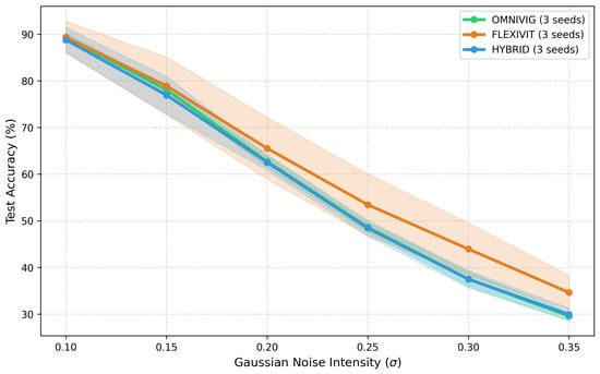
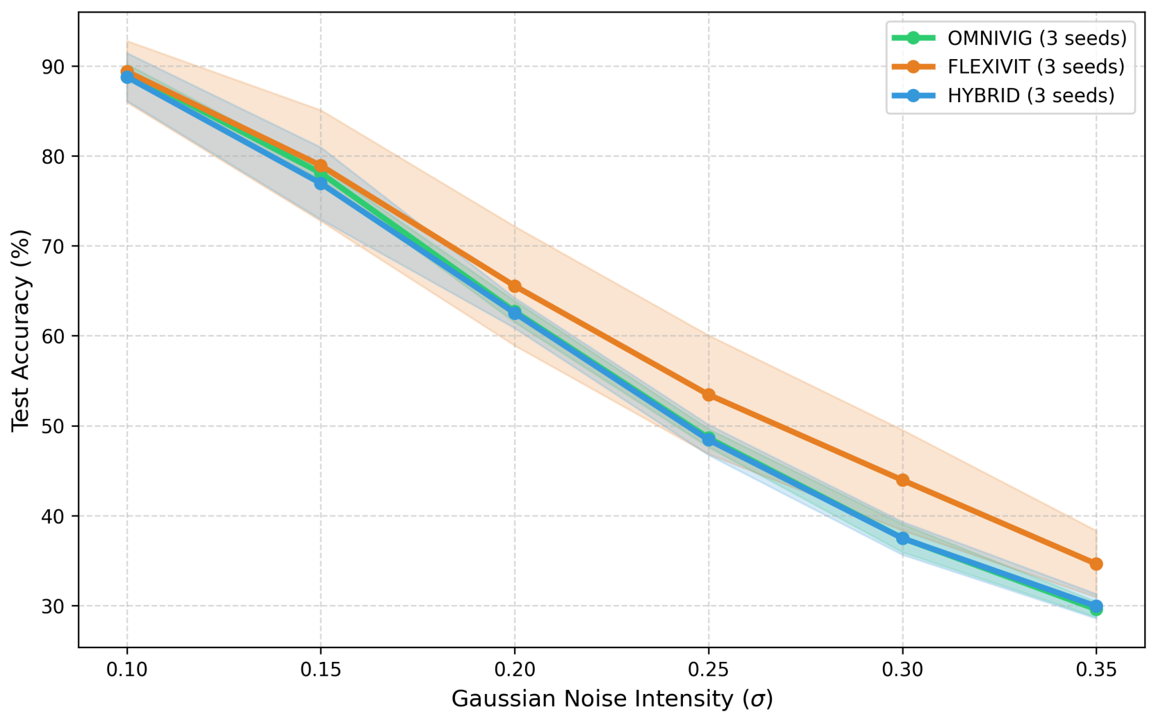
We tested robustness by adding Gaussian noise with standard deviation $\sigma \in [0.10,0.35]$ to the input images, following the common practice of evaluating under synthetic corruptions [83]. The experiment uses Micro-Digits and the three architectures exactly as evaluated in the main experiments (width $C=32$, plain-sum hybrid). For each architecture and each of the three seeds (0, 1, 2), one model was trained for 100 epochs on clean images. Noise was then added to the test images only, and the noisy images were clipped to $[0,1]$. At each of the six noise levels ($\sigma =0.10,0.15,\dots ,0.35$), the test set was corrupted five times with independent noise draws, and the accuracies were averaged over the draws. Figure 4 plots the mean of these values over the three seeds, and Table 15 lists them.

Figure 4. Sensitivity analysis: comparison of test accuracy vs. Gaussian noise intensity ($\sigma$) on Micro-Digits. Each point is the mean over three training seeds of the accuracy averaged over five noise draws; the shaded regions show $\pm 1$ population standard deviation across the three seeds, as in Table 15.

Table 15. Test accuracy (%) on Micro-Digits under Gaussian noise: mean ± population standard deviation across three training seeds, each value averaged over five noise draws.

Architecture	$\mathit{\sigma }=0.10$	$\mathit{\sigma }=0.15$	$\mathit{\sigma }=0.20$	$\mathit{\sigma }=0.25$	$\mathit{\sigma }=0.30$	$\mathit{\sigma }=0.35$
OMNIVIG	$89.4\pm 0.8$	$78.1\pm 0.7$	$62.7\pm 1.2$	$48.6\pm 1.0$	$37.5\pm 1.6$	$29.6\pm 0.9$
FLEXIVIT	$89.4\pm 3.4$	$78.9\pm 6.2$	$65.5\pm 6.6$	$53.4\pm 6.6$	$43.9\pm 5.6$	$34.6\pm 3.7$
HYBRID	$88.8\pm 2.7$	$76.9\pm 4.0$	$62.5\pm 1.7$	$48.4\pm 1.7$	$37.5\pm 1.8$	$29.9\pm 1.4$

5.15.1. Comparative Performance Analysis

All three models lose accuracy as the noise increases (Figure 4, Table 15). At $\sigma =0.10$, they are within one point of each other ($88.8$–$89.4\%$). From $\sigma =0.15$ onwards, FLEXIVIT is the most accurate model, and the hybrid and OMNIVIG follow almost identical curves.

5.15.2. Behaviour at High Noise

At $\sigma =0.35$, FLEXIVIT reaches $34.6\%$, against $29.9\%$ for the hybrid and $29.6\%$ for OMNIVIG; FLEXIVIT is above the hybrid in each of the three seeds. Between $\sigma =0.10$ and $0.35$, FLEXIVIT loses $54.7$ points, the hybrid $58.9$ and OMNIVIG $59.8$.

A plausible reason is that the $3\times 3$ maximum is sensitive to noise: on a noisy image, the maximum of nine pixels is biased upwards, so ${\mathrm{\Delta }}_i$ responds to noise as well as to edges. Attention, which forms weighted averages over all tokens, smooths independent pixel noise. In the plain-sum hybrid, the noisy graph signal is added to the attention output with a fixed weight of one, so the hybrid inherits the sensitivity of the graph branch. A fusion rule that can reduce the weight of the graph branch, such as learnable fusion weights or an input-dependent gate, could avoid this; we do not test this here.

5.15.3. Variability

OMNIVIG is the most consistent model across seeds (standard deviation at most $1.6$ points), whereas FLEXIVIT varies most ($3.4$–$6.6$ points): its seed-1 model ends at $30.1\%$ at $\sigma =0.35$ and its seed-2 model at $39.2\%$. The hybrid lies in between ($1.4$–$4.0$ points). Robustness to noise is therefore a property of the seed as well as of the architecture, so a single trained model per architecture is not enough to rank the models. The variation between noise draws within one model is smaller, $1.6$–$1.9$ points on average.

5.16. Saliency Maps

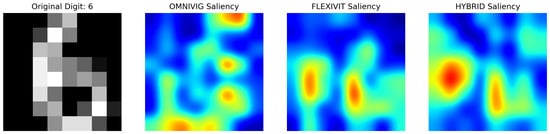
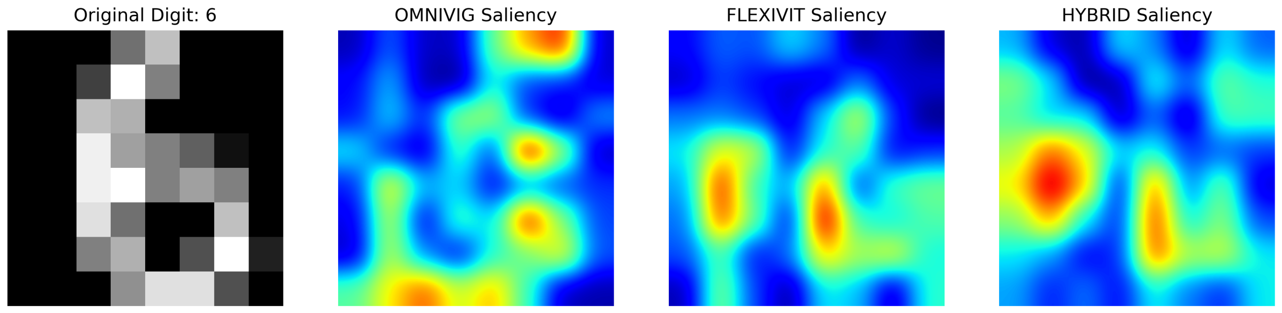
As a qualitative check, we computed gradient-based saliency maps for one sample from the $8\times 8$ digits dataset (Figure 5). The maps use the seed-0 Micro-Digits models of the main experiments (Table 7), so they reflect exactly the evaluated configuration; no separate model was trained. The sample is the first image of the test set, a ‘6’. The saliency of a pixel is the absolute gradient of the predicted class probability with respect to that pixel, normalised to $[0,1]$ for each model. The $8\times 8$ maps are displayed with smooth (Gaussian) interpolation, so each pixel of the input corresponds to one of the $8\times 8$ cells of a map and the rounded shapes are a display effect rather than sub-pixel detail.

Figure 5. Gradient-based saliency maps (absolute gradient of the predicted class probability, normalised to $[0,1]$) of OMNIVIG, FLEXIVIT, and the HYBRID architecture on an $8\times 8$ Micro-Digits test image (a ‘6’), computed with the seed-0 models of the main experiments. The maps are displayed with smooth interpolation over the $8\times 8$ pixel grid.

5.16.1. Visual Comparison

The saliency of OMNIVIG is spread over several separate spots, the strongest in the top-right corner, where the image is background, and along the bottom edge and right side of the loop. This fits a layer that responds to local contrast wherever it occurs, including outside the digit.

The saliency of FLEXIVIT is concentrated in two elongated regions, on the left vertical stroke and inside the loop, i.e., on the two parts that distinguish a ‘6’ from other digits. The saliency of the hybrid has the same two regions, with its strongest response on the left stroke and a broader, weaker response elsewhere. The hybrid’s map is therefore much closer to FLEXIVIT’s than to OMNIVIG’s, which agrees with the quantitative result that the attention branch carries most of the hybrid’s behaviour (Section 5.17).

5.16.2. Limits of the Saliency Analysis

The maps are computed for a single sample and one seed, and are qualitative. They show where each model’s prediction is sensitive to the input, not why the model is correct, and they do not show which branch of the hybrid produces a given pattern. They are not evidence of the accuracy differences reported above.

5.17. Discussion

Four points stand out. Global attention carries most of the accuracy; the graph branch can be added to it at almost no cost and makes training outcomes more stable on some datasets; under the plain sum, the graph branch does not add noise robustness; and an unwarmed latency measurement can mislead by more than an order of magnitude.

5.17.1. What Each Branch Contributes

Because each baseline is the hybrid with one branch removed, the three models form a controlled ablation, and the two comparisons answer different questions.

Removing attention (hybrid vs. OMNIVIG) costs $3.7$ to $15.1$ points of test F1 on every dataset and in every run. One $3\times 3$ neighbourhood followed by global average pooling cannot relate distant parts of the image: in the $8\times 8$ example of Section 3, pixel $(1,1)$ would need seven stacked graph layers to influence pixel $(8,8)$, whereas one attention layer links them directly. The loss is largest where the arrangement of strokes across the whole image matters, as on MNIST ($-15.1$ points) and USPS ($-10.7$ points).

Removing the graph branch (hybrid vs. FLEXIVIT) changes test F1 by between $-2.0$ and $+1.6$ points, with no significant difference across datasets. The hybrid is ahead in every seed on CIFAR-10, Fashion-MNIST and SVHN, i.e., on the textured and natural-image datasets with the most tokens, where an explicit local-contrast signal $\mathrm{\Delta }$ could plausibly help attention, which averages over all tokens and blurs sharp peaks (Section 3.3). It is behind on Micro-Digits, where the whole image has only 64 tokens and attention can already compare every pixel with every other. A second effect is stability: on CIFAR-10 and CIFAR-100 the seed-to-seed standard deviation of the hybrid’s test F1 is $0.73$ and $0.51$ points, against $1.23$ and $1.34$ for FLEXIVIT. For a practitioner who trains a model once, a smaller spread means a smaller risk of an unlucky run. The hybrid’s $C^2+C$ extra parameters could contribute to these effects; a parameter-matched FLEXIVIT would be needed to separate them.

In summary, under late fusion by an unweighted sum, the graph branch is a cheap, low-risk addition but not a source of large gains. In this design, the attention branch never sees the graph output, so the two branches cannot influence each other before the sum. Fusion rules in which the graph features gate or bias the attention scores are the natural next step, and the present results provide the reference against which such designs can be measured.

5.17.2. Latency

The hybrid performs all of FLEXIVIT’s computation plus the graph branch, which adds $0.5$–$3.1\%$ more MACs (Table 1). Under the warm protocol, its latency is within $0.06$ ms of FLEXIVIT’s on every dataset, slightly lower on three and slightly higher on five, which is consistent with the MAC count and within measurement noise. Its training time differs from FLEXIVIT’s by at most $9\%$. OMNIVIG is the only model with a clear speed advantage: on the $32\times 32$ datasets it runs about 7–$10\times$ faster than the attention-based models and trains about 19–$25\times$ faster.

The comparison between the two protocols is a practical result in itself. Under the unwarmed protocol, the per-image latency of the attention-based models on Micro-Digits was $4.1$–$4.8$ ms, about $15\times$ the warm value of $0.27$–$0.32$ ms, and higher than on $96\times 96$ STL-10 images. The inflation comes from a fixed start-up cost divided among only 360 test images; on MNIST, with 10,000 test images, the same cost inflates latency by only about $45\%$. The same protocol makes the hybrid appear faster than FLEXIVIT on five of the eight datasets; this artefact disappears with warm-up. Small-scale studies that time a single predict() call are exposed to the same error.

5.17.3. Robustness to Noise

Over three training seeds (Figure 4), the three models start from similar accuracies at $\sigma =0.10$ ($88.8$–$89.4\%$). As the noise grows, the hybrid follows OMNIVIG closely and ends at $29.9\%$ at $\sigma =0.35$, against $29.6\%$ for OMNIVIG and $34.6\%$ for FLEXIVIT; FLEXIVIT is above the hybrid at $\sigma =0.35$ in each of the three seeds. A plausible explanation is that the plain sum passes the graph branch’s response to noise straight through: the $3\times 3$ maximum is biased upwards on a noisy image, so $\mathrm{\Delta }$ responds to noise as well as to edges, and with an unweighted sum nothing can down-weight it. The result suggests that an adaptive fusion that can reduce the weight of the graph branch under noise is needed for the hybrid to inherit the robustness of attention.

5.17.4. Effect of Resolution

The datasets differ a lot in resolution, and the results differ accordingly:

1.

8 × 8: With only 64 tokens, attention alone can compare every pair of pixels, and FLEXIVIT has the best test F1 ($91.8\%$, against $89.7\%$ for the hybrid and $85.8\%$ for OMNIVIG).

2.

28 × 28 to 32 × 32: With 784–1024 tokens, the hybrid has the best mean test F1 on Fashion-MNIST, CIFAR-10, CIFAR-100 and SVHN, and is ahead in every seed on three of them. MNIST is the exception, with a tie.

3.

96 × 96: After the stride-4 stem, a $3\times 3$ neighbourhood covers a small part of the image. On STL-10, both attention-based models are about 5 points above OMNIVIG, and the hybrid’s lead over FLEXIVIT ($0.6$ points) is within the seed-to-seed variation.

The gap between OMNIVIG and the attention-based models is present at every resolution, which confirms that global context is needed regardless of image size, while any benefit of the local branch appears only at intermediate token counts.

5.17.5. Limitations

The study has several limitations.

(i)

Depth. Each model has a single layer followed by global average pooling, so the results describe the behaviour of the layers rather than of deep networks, and absolute accuracies are low (for example, about $80\%$ on MNIST). Whether the ranking holds when layers are stacked remains open.

(ii)

Training budgets. The budgets are short on some datasets, and no augmentation or schedule is used. SVHN in particular is not learned well by any model (test F1 below $24\%$), so it carries little weight.

(iii)

Statistical power. Three seeds per configuration and eight datasets allow the large effect of attention to be detected, but not a difference of a fraction of a point between the hybrid and FLEXIVIT.

(iv)

Missing controls. There is no parameter-matched FLEXIVIT baseline (for example, with C increased until it has as many parameters as the hybrid) and no study of the neighbourhood size of the graph branch. Since the hybrid has only $C^2+C$ more parameters than FLEXIVIT (1056 to 16,512 depending on C) and is not significantly more accurate, the first control is unlikely to change the conclusions, but both are left to future work.

(v)

Fusion rule. Only the unweighted sum is evaluated in the main experiments. Learnable or input-dependent fusion, and fusion in which the graph features act on the attention scores, are not tested.

(vi)

Scope of the noise and saliency studies. Both use only Micro-Digits; the saliency maps use one sample and one seed.

(vii)

Hardware. Latency is measured on a single cloud GPU (NVIDIA T4, FP32) with Python-level timing. The microcontroller setting that motivates the work is not measured; for it, the parameter counts and analytical MACs are the more relevant figures.

5.17.6. Interpretation

The Wilcoxon tests ($p=0.0078$ against OMNIVIG, $p=0.38$ against FLEXIVIT) show that, under equal training budgets, global attention is what separates the models, and that adding a local graph branch by plain summation neither helps nor hurts significantly across datasets. The hybrid nevertheless keeps practical advantages over FLEXIVIT on part of the benchmark (consistent gains on CIFAR-10, Fashion-MNIST and SVHN, and a smaller spread over seeds on CIFAR-10 and CIFAR-100) for $0.5$–$3.1\%$ more MACs and no measurable change in latency. Whether these effects persist in deeper models, and whether a fusion rule that lets the graph branch guide attention turns them into larger gains, remains to be tested.

6. Conclusions

We presented the Omni-Flex GraphFormer, a hybrid that sums the outputs of a graph branch (OMNIVIG) and a Transformer branch (FLEXIVIT) applied in parallel to the same feature map, and evaluated it as a branch ablation on eight datasets from $8\times 8$ to $96\times 96$ pixels, with three seeds per configuration and equal training budgets within each dataset.

The study gives four answers. First, global attention is essential: removing it lowers test F1 by $3.7$ to $15.1$ points on every dataset and in every run ($p=0.0078$). Second, adding the local graph branch to attention is almost free (4–$6\%$ more parameters, $0.5$–$3.1\%$ more MACs, the same measured latency) and safe: the hybrid has the best mean test F1 on six of the eight datasets, is ahead in every seed on CIFAR-10, Fashion-MNIST and SVHN, and has a smaller spread over seeds on CIFAR-10 and CIFAR-100, although the difference from FLEXIVIT across datasets is not significant ($p=0.38$). Third, under Gaussian noise on Micro-Digits, the summed hybrid degrades like the graph branch, while the Transformer branch is the most robust model, so plain summation does not transfer the robustness of attention. Fourth, latency must be measured with warm-up and repeated passes: a single unwarmed call overstated per-image latency by up to $15\times$ on the smallest test set and produced speed differences between FLEXIVIT and the hybrid that do not exist.

These results establish a measured baseline for parallel graph–attention fusion and locate its bottleneck in the fusion rule. Future work will replace the unweighted sum with fusion in which the graph features gate or bias the attention scores, add a parameter-matched baseline and a study of the neighbourhood size, evaluate deeper models, test the flexible and adaptive patching of FlexiViT within the hybrid, and apply the approach to 3D point clouds and video.

References

- Dosovitskiy, A.; Beyer, L.; Kolesnikov, A.; Weissenborn, D.; Zhai, X.; Unterthiner, T.; Dehghani, M.; Minderer, M.; Heigold, G.; Gelly, S.; et al. An Image is Worth 16x16 Words: Transformers for Image Recognition at Scale. In Proceedings of the International Conference on Learning Representations (ICLR), Virtual Event, 3–7 May 2021. [Google Scholar]
- Han, K.; Wang, Y.; Guo, J.; Tang, Y.; Wu, E. Vision GNN: An Image is Worth Graph of Nodes. Adv. Neural Inf. Process. Syst. 2022, 35, 8291–8303. [Google Scholar] [CrossRef] [Scilit]
- Munir, M.; Avery, W.; Marculescu, R. MobileViG: Graph-Based Sparse Attention for Mobile Vision Applications. In Proceedings of the IEEE/CVF Conference on Computer Vision and Pattern Recognition Workshops (CVPRW); IEEE: Piscataway, NJ, USA, 2023; pp. 2211–2219. [Google Scholar]
- Avery, W.; Munir, M.; Marculescu, R. Scaling Graph Convolutions for Mobile Vision. In Proceedings of the IEEE/CVF Conference on Computer Vision and Pattern Recognition Workshops (CVPRW); IEEE: Piscataway, NJ, USA, 2024; pp. 5857–5865. [Google Scholar]
- Munir, M.; Avery, W.; Rahman, M.M.; Marculescu, R. GreedyViG: Dynamic Axial Graph Construction for Efficient Vision GNNs. In Proceedings of the IEEE/CVF Conference on Computer Vision and Pattern Recognition (CVPR); IEEE: Piscataway, NJ, USA, 2024; pp. 6118–6127. [Google Scholar]
- Munir, M.; Rahman, M.M.; Marculescu, R. AdaptViG: Adaptive Vision GNN with Exponential Decay Gating. In Proceedings of the IEEE/CVF Winter Conference on Applications of Computer Vision (WACV); IEEE: Piscataway, NJ, USA, 2026. [Google Scholar]
- Beyer, L.; Izmailov, P.; Kolesnikov, A.; Caron, M.; Kornblith, S.; Zhai, X.; Minderer, M.; Tschannen, M.; Alabdulmohsin, I.; Pavetic, F. FlexiViT: One Model for All Patch Sizes. In Proceedings of the IEEE/CVF Conference on Computer Vision and Pattern Recognition (CVPR); IEEE: Piscataway, NJ, USA, 2023. [Google Scholar]
- Bruna, J.; Zaremba, W.; Szlam, A.; LeCun, Y. Spectral Networks and Deep Locally Connected Networks on Graphs. arXiv 2013, arXiv:1312.6203. [Google Scholar]
- Defferrard, M.; Bresson, X.; Vandergheynst, P. Convolutional Neural Networks on Graphs with Fast Localized Spectral Filtering. In Advances in Neural Information Processing Systems; NeurIPS: Red Hook, NY, USA, 2016; Volume 29. [Google Scholar]
- Kipf, T.N.; Welling, M. Semi-Supervised Classification with Graph Convolutional Networks. In Proceedings of the International Conference on Learning Representations (ICLR), Toulon, France, 24–26 April 2017. [Google Scholar]
- Hamilton, W.; Ying, Z.; Leskovec, J. Inductive Representation Learning on Large Graphs. In Advances in Neural Information Processing Systems; NeurIPS: Red Hook, NY, USA, 2017; Volume 30. [Google Scholar]
- Veličković, P.; Cucurull, G.; Casanova, A.; Romero, A.; Liò, P.; Bengio, Y. Graph Attention Networks. In Proceedings of the International Conference on Learning Representations (ICLR), Vancouver, BC, Canada, 30 April–3 May 2018. [Google Scholar]
- Brody, S.; Alon, U.; Yahav, E. How Attentive are Graph Attention Networks? In Proceedings of the International Conference on Learning Representations (ICLR), Virtual Event, 25–29 April 2022. [Google Scholar]
- Shi, W.; Rajkumar, R. Point-GNN: Graph Neural Network for 3D Object Detection in a Point Cloud. In Proceedings of the IEEE/CVF Conference on Computer Vision and Pattern Recognition (CVPR); IEEE: Piscataway, NJ, USA, 2020. [Google Scholar]
- Wang, Y.; Sun, Y.; Liu, Z.; Sarma, S.E.; Bronstein, M.M.; Solomon, J.M. Dynamic Graph CNN for Learning on Point Clouds. ACM Trans. Graph. 2019, 38, 1–12. [Google Scholar] [CrossRef] [Scilit]
- Ying, Z.; You, J.; Morris, C.; Ren, X.; Hamilton, W.; Leskovec, J. Hierarchical Graph Representation Learning with Differentiable Pooling. In Advances in Neural Information Processing Systems; NeurIPS: Red Hook, NY, USA, 2018; Volume 31. [Google Scholar]
- Lee, J.; Lee, I.; Kang, J. Self-Attention Graph Pooling. In Proceedings of the International Conference on Machine Learning (ICML), Long Beach, CA, USA, 9–15 June 2019. [Google Scholar]
- Gao, H.; Ji, S. Graph U-Nets. In Proceedings of the International Conference on Machine Learning (ICML), Long Beach, CA, USA, 9–15 June 2019. [Google Scholar]
- Chiang, W.L.; Liu, X.; Si, S.; Li, Y.; Bengio, S.; Hsieh, C.J. Cluster-GCN: An Efficient Algorithm for Training Deep and Large Graph Convolutional Networks. In Proceedings of the 25th ACM SIGKDD International Conference on Knowledge Discovery & Data Mining (KDD), Anchorage, AK, USA, 4–8 August 2019. [Google Scholar]
- Xu, K.; Hu, W.; Leskovec, J.; Jegelka, S. How Powerful are Graph Neural Networks? In Proceedings of the International Conference on Learning Representations (ICLR), New Orleans, LA, USA, 6–9 May 2019. [Google Scholar]
- Li, Q.; Han, Z.; Wu, X.M. Deeper Insights into Graph Convolutional Networks for Semi-Supervised Learning. In Proceedings of the AAAI Conference on Artificial Intelligence, New Orleans, LA, USA, 2–7 February 2018; Volume 32. [Google Scholar]
- Xu, K.; Li, C.; Tian, Y.; Sonobe, T.; Kawarabayashi, K.; Jegelka, S. Representation Learning on Graphs with Jumping Knowledge Networks. In Proceedings of the International Conference on Machine Learning (ICML), Stockholm, Sweden, 10–15 July 2018. [Google Scholar]
- Li, G.; Müller, M.; Thabet, A.; Ghanem, B. DeepGCNs: Can GCNs Go as Deep as CNNs? In Proceedings of the IEEE/CVF International Conference on Computer Vision (ICCV); IEEE: Piscataway, NJ, USA, 2019. [Google Scholar]
- Li, G.; Müller, M.; Qian, G.; Delgadillo, I.C.; Abualshour, A.; Thabet, A.; Ghanem, B. DeepGCNs: Making GCNs Go as Deep as CNNs. IEEE Trans. Pattern Anal. Mach. Intell. 2023, 45, 6923–6939. [Google Scholar] [CrossRef] [Scilit] [PubMed]
- Zhao, L.; Akoglu, L. PairNorm: Tackling Oversmoothing in GNNs. In Proceedings of the International Conference on Learning Representations (ICLR), Virtual Event, 26 April–1 May 2020. [Google Scholar]
- Rong, Y.; Huang, W.; Xu, T.; Huang, J. DropEdge: Towards Deep Graph Convolutional Networks on Node Classification. In Proceedings of the International Conference on Learning Representations (ICLR), Virtual Event, 26 April–1 May 2020. [Google Scholar]
- Dwivedi, V.P.; Bresson, X. A Generalization of Transformer Networks to Graphs. arXiv 2020, arXiv:2012.09699. [Google Scholar]
- Yun, S.; Jeong, M.; Kim, R.; Kang, J.; Kim, H.J. Graph Transformer Networks. In Advances in Neural Information Processing Systems; NeurIPS: Red Hook, NY, USA, 2019; Volume 32. [Google Scholar]
- Touvron, H.; Cord, M.; Douze, M.; Massa, F.; Sablayrolles, A.; Jégou, H. Training Data-Efficient Image Transformers & Distillation Through Attention. In Proceedings of the International Conference on Machine Learning (ICML), Virtual Event, 18–24 July 2021. [Google Scholar]
- Touvron, H.; Cord, M.; Sablayrolles, A.; Synnaeve, G.; Jégou, H. Going Deeper with Image Transformers. In Proceedings of the IEEE/CVF International Conference on Computer Vision (ICCV); IEEE: Piscataway, NJ, USA, 2021. [Google Scholar]
- Liu, Z.; Lin, Y.; Cao, Y.; Hu, H.; Wei, Y.; Zhang, Z.; Lin, S.; Guo, B. Swin Transformer: Hierarchical Vision Transformer Using Shifted Windows. In Proceedings of the IEEE/CVF International Conference on Computer Vision (ICCV); IEEE: Piscataway, NJ, USA, 2021. [Google Scholar]
- Liu, Z.; Hu, H.; Lin, Y.; Yao, Z.; Xie, Z.; Wei, Y.; Ning, J.; Cao, Y.; Zhang, Z.; Dong, L.; et al. Swin Transformer V2: Scaling Up Capacity and Resolution. In Proceedings of the IEEE/CVF Conference on Computer Vision and Pattern Recognition (CVPR); IEEE: Piscataway, NJ, USA, 2022. [Google Scholar]
- Wang, W.; Xie, E.; Li, X.; Fan, D.P.; Song, K.; Liang, D.; Lu, T.; Luo, P.; Shao, L. Pyramid Vision Transformer: A Versatile Backbone for Dense Prediction Without Convolutions. In Proceedings of the IEEE/CVF International Conference on Computer Vision (ICCV); IEEE: Piscataway, NJ, USA, 2021. [Google Scholar]
- Wang, W.; Xie, E.; Li, X.; Fan, D.P.; Song, K.; Liang, D.; Lu, T.; Luo, P.; Shao, L. PVTv2: Improved Baselines with Pyramid Vision Transformer. Comput. Vis. Media 2022, 8, 415–424. [Google Scholar] [CrossRef] [Scilit]
- Yuan, L.; Chen, Y.; Wang, T.; Yu, W.; Shi, Y.; Jiang, Z.H.; Tay, F.E.; Feng, J.; Yan, S. Tokens-to-Token ViT: Training Vision Transformers from Scratch on ImageNet. In Proceedings of the IEEE/CVF International Conference on Computer Vision (ICCV); IEEE: Piscataway, NJ, USA, 2021. [Google Scholar]
- Han, K.; Xiao, A.; Wu, E.; Guo, J.; Xu, C.; Wang, Y. Transformer in Transformer. In Advances in Neural Information Processing Systems; NeurIPS: Red Hook, NY, USA, 2021; Volume 34. [Google Scholar]
- Yang, R.; Ma, H.; Wu, J.; Tang, Y.; Xiao, X.; Zheng, M.; Li, X. ScalableViT: Rethinking the Context-oriented Generalization of Vision Transformer. In Proceedings of the European Conference on Computer Vision (ECCV), Tel Aviv, Israel, 23–27 October 2022. [Google Scholar]
- Chen, C.F.R.; Fan, Q.; Panda, R. CrossViT: Cross-Attention Multi-Scale Vision Transformer for Image Classification. In Proceedings of the IEEE/CVF International Conference on Computer Vision (ICCV); IEEE: Piscataway, NJ, USA, 2021. [Google Scholar]
- Ali, A.; Touvron, H.; Caron, M.; Bojanowski, P.; Douze, M.; Joulin, A.; Laptev, I.; Neverova, N.; Synnaeve, G.; Verbeek, J.; et al. XCiT: Cross-Covariance Image Transformers. In Advances in Neural Information Processing Systems; NeurIPS: Red Hook, NY, USA, 2021; Volume 34. [Google Scholar]
- Oquab, M.; Darcet, T.; Moutakanni, T.; Vo, H.; Szafraniec, M.; Khalidov, V.; Fernandez, P.; Haziza, D.; Massa, F.; El-Nouby, A.; et al. DINOv2: Learning Robust Visual Features Without Supervision. Trans. Mach. Learn. Res. 2024. Available online: https://openreview.net/forum?id=a68SUt6zFt (accessed on 26 October 2026).
- Mehta, S.; Rastegari, M. MobileViT: Light-Weight, General-Purpose, and Mobile-Friendly Vision Transformer. In Proceedings of the International Conference on Learning Representations (ICLR), Virtual Event, 25–29 April 2022. [Google Scholar]
- Mehta, S.; Rastegari, M. Separable Self-Attention for Mobile Vision Transformers (MobileViTv2). arXiv 2022, arXiv:2206.02680. [Google Scholar]
- Vasu, P.K.A.; Gabriel, J.; Zhu, J.; Tuzel, O.; Ranjan, A. FastViT: A Fast Hybrid Vision Transformer Using Structural Reparameterization. In Proceedings of the IEEE/CVF International Conference on Computer Vision (ICCV); IEEE: Piscataway, NJ, USA, 2023. [Google Scholar]
- Chen, X.; Liu, Z.; Tang, H.; Yi, L.; Zhao, H.; Han, S. SparseViT: Revisiting Activation Sparsity for Efficient High-Resolution Vision Transformer. In Proceedings of the IEEE/CVF Conference on Computer Vision and Pattern Recognition (CVPR); IEEE: Piscataway, NJ, USA, 2023. [Google Scholar]
- Ryoo, M.S.; Piergiovanni, A.; Arnab, A.; Dehghani, M.; Angelova, A. TokenLearner: Adaptive Space-Time Tokenization for Videos. In Advances in Neural Information Processing Systems; NeurIPS: Red Hook, NY, USA, 2021; Volume 34. [Google Scholar]
- Li, K.; Wang, Y.; Zhang, J.; Gao, P.; Song, G.; Liu, Y.; Li, H.; Qiao, Y. UniFormer: Unifying Convolution and Self-Attention for Visual Recognition. IEEE Trans. Pattern Anal. Mach. Intell. 2023, 45, 12581–12600. [Google Scholar] [CrossRef] [Scilit] [PubMed]
- Li, Y.; Wu, C.Y.; Fan, H.; Mangalam, K.; Xiong, B.; Malik, J.; Feichtenhofer, C. MViTv2: Improved Multiscale Vision Transformers for Classification and Detection. In Proceedings of the IEEE/CVF Conference on Computer Vision and Pattern Recognition (CVPR); IEEE: Piscataway, NJ, USA, 2022. [Google Scholar]
- d’Ascoli, S.; Touvron, H.; Leavitt, M.L.; Morcos, A.S.; Biroli, G.; Sagun, L. ConViT: Improving Vision Transformers with Soft Convolutional Inductive Biases. In Proceedings of the International Conference on Machine Learning (ICML), Virtual Event, 18–24 July 2021. [Google Scholar]
- Guo, J.; Han, K.; Wu, H.; Tang, Y.; Chen, X.; Wang, Y.; Xu, C. CMT: Convolutional Neural Networks Meet Vision Transformers. In Proceedings of the IEEE/CVF Conference on Computer Vision and Pattern Recognition (CVPR); IEEE: Piscataway, NJ, USA, 2022. [Google Scholar]
- Wu, H.; Xiao, B.; Codella, N.; Liu, M.; Dai, X.; Yuan, L.; Zhang, L. CvT: Introducing Convolutions to Vision Transformers. In Proceedings of the IEEE/CVF International Conference on Computer Vision (ICCV); IEEE: Piscataway, NJ, USA, 2021. [Google Scholar]
- Graham, B.; El-Nouby, A.; Touvron, H.; Stock, P.; Joulin, A.; Jégou, H.; Douze, M. LeViT: A Vision Transformer in ConvNet’s Clothing for Faster Inference. In Proceedings of the IEEE/CVF International Conference on Computer Vision (ICCV); IEEE: Piscataway, NJ, USA, 2021. [Google Scholar]
- Srinivas, A.; Lin, T.Y.; Parmar, N.; Shlens, J.; Abbeel, P.; Vaswani, A. Bottleneck Transformers for Visual Recognition. In Proceedings of the IEEE/CVF Conference on Computer Vision and Pattern Recognition (CVPR); IEEE: Piscataway, NJ, USA, 2021. [Google Scholar]
- Dai, Z.; Liu, H.; Le, Q.V.; Tan, M. CoAtNet: Marrying Convolution and Attention for All Data Sizes. In Advances in Neural Information Processing Systems; NeurIPS: Red Hook, NY, USA, 2021; Volume 34. [Google Scholar]
- Li, Y.; Zhang, K.; Cao, J.; Timofte, R.; Van Gool, L. LocalViT: Bringing Locality to Vision Transformers. arXiv 2021, arXiv:2104.05707. [Google Scholar]
- Ying, C.; Cai, T.; Luo, S.; Zheng, S.; Ke, G.; He, D.; Shen, Y.; Liu, T.Y. Do Transformers Really Perform Bad for Graph Representation? In Advances in Neural Information Processing Systems; NeurIPS: Red Hook, NY, USA, 2021; Volume 34. [Google Scholar]
- Rao, Y.; Zhao, W.; Zhu, Z.; Lu, J.; Zhou, J. Global Filter Networks for Image Classification. In Advances in Neural Information Processing Systems; NeurIPS: Red Hook, NY, USA, 2021; Volume 34. [Google Scholar]
- Wu, Z.; Jain, P.; Wright, M.; Mirhoseini, A.; Gonzalez, J.E.; Stoica, I. Representing Long-Range Context for Graph Neural Networks with Global Attention. In Advances in Neural Information Processing Systems; NeurIPS: Red Hook, NY, USA, 2021; Volume 34. [Google Scholar]
- Kim, J.; Nguyen, T.D.; Min, S.; Cho, S.; Lee, M.; Lee, H.; Hong, S. Pure Transformers are Powerful Graph Learners. In Advances in Neural Information Processing Systems; NeurIPS: Red Hook, NY, USA, 2022; Volume 35. [Google Scholar]
- Rampášek, L.; Galkin, M.; Dwivedi, V.P.; Luu, A.T.; Wolf, G.; Beaini, D. Recipe for a General, Powerful, Scalable Graph Transformer. In Advances in Neural Information Processing Systems; NeurIPS: Red Hook, NY, USA, 2022; Volume 35. [Google Scholar]
- Pan, J.; Bulat, A.; Tan, F.; Zhu, X.; Dudziak, Ł.; Li, H.; Tzimiropoulos, G.; Martinez, B. EdgeViT: Competing Light-weight CNNs on Mobile Devices with Vision Transformers. In Proceedings of the European Conference on Computer Vision (ECCV), Tel Aviv, Israel, 23–27 October 2022. [Google Scholar]
- Wu, Q.; Zhao, W.; Li, Z.; Wipf, D.P.; Yan, J. NodeFormer: A Scalable Graph Structure Learning Transformer for Node Classification. In Advances in Neural Information Processing Systems; NeurIPS: Red Hook, NY, USA, 2022; Volume 35. [Google Scholar]
- Han, K.; Wang, Y.; Chen, H.; Chen, X.; Guo, J.; Liu, Z.; Tang, Y.; Xiao, A.; Xu, C.; Xu, Y.; et al. A Survey on Vision Transformer. IEEE Trans. Pattern Anal. Mach. Intell. 2023, 45, 87–110. [Google Scholar] [CrossRef] [Scilit] [PubMed]
- Tay, Y.; Dehghani, M.; Bahri, D.; Metzler, D. Efficient Transformers: A Survey. ACM Comput. Surv. 2022, 55, 109. [Google Scholar] [CrossRef] [Scilit]
- Dehghani, M.; Arnab, A.; Beyer, L.; Vaswani, A.; Tay, Y. The Efficiency Misnomer. In Proceedings of the International Conference on Learning Representations (ICLR), Virtual Event, 25–29 April 2022. [Google Scholar]
- Papa, L.; Russo, P.; Amerini, I.; Zhou, L. A Survey on Efficient Vision Transformers: Algorithms, Techniques, and Performance Benchmarking. IEEE Trans. Pattern Anal. Mach. Intell. 2024, 46, 7682–7700. [Google Scholar] [CrossRef] [Scilit] [PubMed]
- Partovi Nia, V.; Ghaffari, A.; Zolnouri, M.; Savaria, Y. Rethinking Pareto Frontier for Performance Evaluation of Deep Neural Networks. In Proceedings of the ICML 2022 Workshop on Hardware-Aware Efficient Training (HAET), Baltimore, MD, USA, 17–23 July 2022. [Google Scholar]
- Tan, M.; Chen, B.; Pang, R.; Vasudevan, V.; Sandler, M.; Howard, A.; Le, Q.V. MnasNet: Platform-Aware Neural Architecture Search for Mobile. In Proceedings of the IEEE/CVF Conference on Computer Vision and Pattern Recognition (CVPR); IEEE: Piscataway, NJ, USA, 2019. [Google Scholar]
- Cai, H.; Zhu, L.; Han, S. ProxylessNAS: Direct Neural Architecture Search on Target Task and Hardware. In Proceedings of the International Conference on Learning Representations (ICLR), New Orleans, LA, USA, 6–9 May 2019. [Google Scholar]
- Yang, T.J.; Chen, Y.H.; Sze, V. Designing Energy-Efficient Convolutional Neural Networks Using Energy-Aware Pruning. In Proceedings of the IEEE Conference on Computer Vision and Pattern Recognition (CVPR); IEEE: Piscataway, NJ, USA, 2017. [Google Scholar]
- Reddi, V.J.; Cheng, C.; Kanter, D.; Mattson, P.; Schmuelling, G.; Wu, C.J.; Anderson, B.; Breughe, M.; Charlebois, M.; Chou, W.; et al. MLPerf Inference Benchmark. In Proceedings of the 47th International Symposium on Computer Architecture (ISCA), Virtual Event, 30 May–3 June 2020. [Google Scholar]
- Banbury, C.; Reddi, V.J.; Lam, M.; Fu, W.; Fazel, A.; Holleman, J.; Huang, X.; Hurtado, R.; Kanter, D.; Lokhmotov, A.; et al. Benchmarking TinyML Systems: Challenges and Direction. arXiv 2020, arXiv:2003.04821. [Google Scholar]
- Schwartz, R.; Dodge, J.; Smith, N.A.; Etzioni, O. Green AI. Commun. ACM 2020, 63, 54–63. [Google Scholar] [CrossRef] [Scilit]
- Patterson, D.; Gonzalez, J.; Le, Q.; Liang, C.; Munguia, L.M.; Rothchild, D.; So, D.; Texier, M.; Dean, J. Carbon Emissions and Large Neural Network Training. arXiv 2021, arXiv:2104.10350. [Google Scholar]
- Lacoste, A.; Luccioni, A.; Schmidt, V.; Dandres, T. Quantifying the Carbon Emissions of Machine Learning. In Proceedings of the Workshop on Tackling Climate Change with Machine Learning at NeurIPS, Vancouver, BC, Canada, 14 December 2019. [Google Scholar]
- Demšar, J. Statistical Comparisons of Classifiers over Multiple Data Sets. J. Mach. Learn. Res. 2006, 7, 1–30. [Google Scholar]
- Wilcoxon, F. Individual Comparisons by Ranking Methods. Biom. Bull. 1945, 1, 80–83. [Google Scholar] [CrossRef] [Scilit]
- García, S.; Molina, D.; Lozano, M.; Herrera, F. A Study on the Use of Non-Parametric Tests for Analyzing the Evolutionary Algorithms’ Behaviour: A Case Study on the CEC’2005 Special Session on Real Parameter Optimization. J. Heuristics 2009, 15, 617–644. [Google Scholar] [CrossRef] [Scilit]
- García, S.; Fernández, A.; Luengo, J.; Herrera, F. Advanced Nonparametric Tests for Multiple Comparisons in the Design of Experiments in Computational Intelligence and Data Mining: Experimental Analysis of Power. Inf. Sci. 2010, 180, 2044–2064. [Google Scholar] [CrossRef] [Scilit]
- Hoefler, T.; Belli, R. Scientific Benchmarking of Parallel Computing Systems: Twelve Ways to Tell the Masses When Reporting Performance Results. In Proceedings of the International Conference for High Performance Computing, Networking, Storage and Analysis (SC ’15), Austin, TX, USA, 15–20 November 2015. Article 73. [Google Scholar]
- Howard, A.G.; Zhu, M.; Chen, B.; Kalenichenko, D.; Wang, W.; Weyand, T.; Andreetto, M.; Adam, H. MobileNets: Efficient Convolutional Neural Networks for Mobile Vision Applications. arXiv 2017, arXiv:1704.04861. [Google Scholar]
- Iandola, F.N.; Han, S.; Moskewicz, M.W.; Ashraf, K.; Dally, W.J.; Keutzer, K. SqueezeNet: AlexNet-Level Accuracy with 50x Fewer Parameters and Less Than 0.5MB Model Size. arXiv 2016, arXiv:1602.07360. [Google Scholar]
- Vaswani, A.; Shazeer, N.; Parmar, N.; Uszkoreit, J.; Jones, L.; Gomez, A.N.; Kaiser, Ł.; Polosukhin, I. Attention is All You Need. In Advances in Neural Information Processing Systems; NeurIPS: Red Hook, NY, USA, 2017; Volume 30. [Google Scholar]
- Hendrycks, D.; Dietterich, T. Benchmarking Neural Network Robustness to Common Corruptions and Perturbations. In Proceedings of the International Conference on Learning Representations (ICLR), New Orleans, LA, USA, 6–9 May 2019. [Google Scholar]
Disclaimer/Publisher’s Note: The statements, opinions and data contained in all publications are solely those of the individual author(s) and contributor(s) and not of MDPI and/or the editor(s). MDPI and/or the editor(s) disclaim responsibility for any injury to people or property resulting from any ideas, methods, instructions or products referred to in the content. |
© 2026 by the authors. Licensee MDPI, Basel, Switzerland. This article is an open access article distributed under the terms and conditions of the Creative Commons Attribution (CC BY) license.