


Abstract
Gait can demonstrate the motion characteristics of individuals and is used as a fundamental basis for assessing their physical conditions. In this paper, a new approach to gait analysis is presented by using a chest-mounted camera to collect images captured from a first-person perspective. After spatial gait measurements and temporal gait descriptors are extracted from those images, accurate gait parameters corresponding to personal medical information can be computed. Unlike traditional devices that need to stick sensors to the observed parts of the body, gait patterns can be obtained from a chest-mounted camera by the proposed new method. To prove the validity and robustness of this new approach for gait analysis, we considered various factors affecting the accuracy of gait parameters, including different individuals, genders, and ages. Additionally, the reference-system comparison and robustness experiments were conducted. Experimental results showed that this new approach can obtain accurate gait parameters close to those of expensive devices. Therefore, this approach can be further used for gait analysis to improve the quality of clinical medicine. This can also provide the advantage of convenience and suitability to apply for long-term healthcare at home.
1. Introduction
Gait Analysis has gained much popularity for its applications in clinical diagnosis, rehabilitation approaches, biometric identification, robotics, and sports. Abdullah et al. [1] provided a systematic literature overview of multibody musculoskeletal (MSK) modeling methodologies and their applications for gait analysis. Li et al. [2] presented a gait recognition model using spatio-temporal slice features to associate human body characteristics from top to bottom. Sethi et al. [3] summarized the history, parameters, and approaches for gait analysis in the past 20 years. Aboutorabi et al. [4] mentioned that aging can affect gait parameters of elderly citizens. Generally, subjective assessment of gait was conducted by health experts; however, gait analysis can now be performed objectively and empirically for better and more reliable assessment. Walking mainly involves the upright posture and movement of the human body. Guan et al. [5] analyzed the pelvis–hip biomechanics, trunk, and lower limb muscle activity patterns between healthy people during walking. Therefore, walking is a complex exercise of lower limb coordination involving bones, joints, and muscles. From the perspective of gait pathology, disease status changes the coordination, balance, and interaction of muscles, bones, nerves, and even joints, resulting in gait abnormalities. These can be broken down by gait analysis and used for correct diagnosis and appropriate treatment in clinical medicine.
Brownjohn et al. [6] and Sahnaci et al. [7] illustrated that there are differences in gait between various people. The classification of gait varies according to age; Bisi and Satgni [8] demonstrated the change in gait pattern during the six months after the child begins to walk alone. Imms and Edholm [9] mentioned that older people walk slower because the energy consumption of their hip and knee joints is higher than that of younger people, but this deceleration is not due to the slower cadence but to the shortening of the stride length [10]. There are also different gait patterns for different genders. Kerrigan et al. [11] showed that women tend to have a greater angular rotation and movement of the pelvis than men when walking, but many people have questioned this stereotype until Muro-De-La-Herran et al. [12] in 2014 used statistical analysis to prove that gait patterns do vary between sexes.
Before gait measurement devices were available, doctors normally collected gait parameters by visual inspection. Since there are many subtle changes that cannot be seen accurately and it is highly dependent on the experience of doctors, the accuracy of gait data measured is restricted. After that, measurement devices such as RGB cameras configured from a third-person perspective are used to collect gait video streams for further analysis [13]. However, the camera must be placed in a fixed position, so the shooting location is often confined, and the number of steps that can be captured is limited [14]. When the test subject knows that he is being filmed, the walking posture may also change unconsciously, resulting in deviations. Therefore, the alternative use of motion capture systems or plantar pressure measurement can solve those problems, and the test subjects can go out of a specific area to observe their walking posture. Nevertheless, most of the sensors, such as gyroscopes and accelerometers, need to be mounted on the observed parts of the body with wires, so the test subjects still cannot move too far away from a specific position, and the gait parameters cannot always be measured regardless of location [15].
For the applications of clinical medicine, the gait data of some patients are collected in medical institutions using relevant equipment such as RGB cameras configured from a third-person perspective or motion capture systems with special arrangement [16]. Particularly, the use of motion capture devices for gait detection relies on the assistance of professionals when setting up and wearing them in advance, so gait observation is still mainly carried out in hospitals. Therefore, an alternative solution that can measure anytime, anywhere, even in the daily environment at home, and whose equipment is simple to operate, becomes essential for collecting personal gait data.
To collect data using multiple externally positioned cameras synchronously, the stability of filming conditions should be assured, and further image integration is needed. Also, the collected data from wearable devices need to go through multiple steps of transmission before data analysis. At first, the gait data is received by the sensors, and then the sensors transmit the information to the computer, where data analysis is achieved. Furthermore, gyroscopes and accelerometers generate cumulative errors due to constant changes in direction and position, and frequent repositioning is necessary. Although many methods have been proposed to analyze gait using externally positioned cameras and wearable devices [1,4], related approaches for analyzing gait using first-person cameras are rare [17]. The advantage of using first-person cameras is that the test subject only needs to wear a camera and record the image changes in front of the body when walking. After the video is completed, the video is transmitted to the computer, and the walking posture can be analyzed. This method can not only solve the problem of limited space but also be easier than the traditional method in terms of data analysis and collection.
Note that the distinction we intend to make is not between different types of cameras, but between an externally observed third-person configuration and the body-worn first-person imaging configuration investigated in this study. In summary, the main contributions of first-person camera-based gait analysis are
- (1)
- Overcome the problem of limited space for data collection.
- (2)
- Develop devices that are simple and easy to carry.
- (3)
- The system can automatically analyze the gait information from the video.
- (4)
- The subject’s walking habits can be deduced from the data.
2. Related Work
There are currently many devices for analyzing gait, which can be divided into two types of devices: wearable and non-wearable, according to the contact relationship between the device and the human body. In this paper, the goal is to emphasize the difference between an externally observed third-person configuration and the body-worn first-person imaging configuration. Wang et al. [18] synthesized three main methods for gait analysis: image processing, ground-based sensors (e.g., foot pressure measurement version), and sensors placed on the body. Image processing is the use of images taken by RGB cameras configured from a third-person perspective as the dataset for analysis, such as Huang [19], who used the spatial and temporal changes in the body contour of an individual’s walking to do gait recognition. Also, Nixon and Carter [20] achieved biometric identification based on an individual’s different gait patterns. Any device that can be worn on the human body can be called a wearable device, such as a smart sports watch, mobile phone, etc. Kourogi and Kurata [21] combined a first-person camera with a gyroscope and an accelerometer to identify gait and the person’s position. There are examples of first-person cameras such as Google Glass, GoPro, or cipher cameras, which can be worn on the body. Using the first-person camera for video recording, the action process of each target can be obtained without being limited by a small space. Betancourt et al. [22] summarized the development of first-person cameras from 1997 to 2014. Rota et al. [23] summarized several gait indicators to analyze patients with abnormal walking. In addition to the treatment and rehabilitation of physical conditions, gait analysis can also be used to predict diseases. Veerbeek [24] uses gait status changes to predict recovery after stroke and treat it early within 72 h after stroke. Wood et al. [25] studied the prediction of fall probability in Parkinson’s patients. This is also helpful for home-based elderly care; Kearns et al. [26] adopted gait detection to identify changes in the physiological status of the elderly and to reduce the risk of falls.
2.1. Gait Cycle
Gait patterns continue to repeat consecutive movements, and each consecutive movement is defined as a gait cycle. Minett [27] illustrates the repetitiveness of the gait cycle and subdivides it into a swing phase and a support phase for one foot. However, these gait cycles are all classified by physical movements. Also, the value of gravity from accelerometer signals is used to distinguish gait cycles [28]. When the human body begins to walk, the body first steps out with one foot, and the other foot lifts and takes off. In this process, the body loses balance. To pull back the balance and move forward, the other foot quickly moves forward and lands on the ground. Based on the definition, the process from the foot leaving the ground until landing on the ground is called one step, and the length is named step length. After the second foot finishes the process of one step, this is called one stride, and the distance is named stride length. From the perspective of the timeline, the time taken for this repetitive action is called a gait cycle.
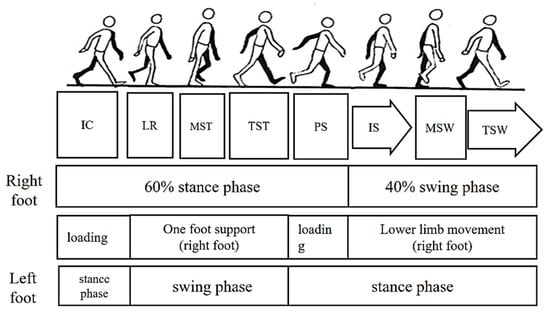
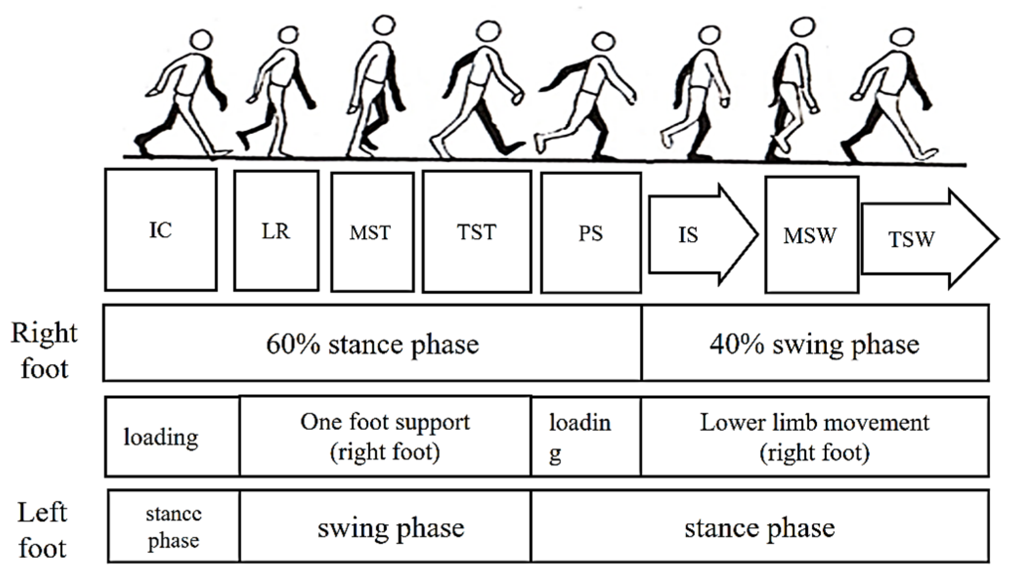
In the process of walking, the left/right foot touches the ground for a period, and the other period is in the air. As shown in Figure 1, the period when the foot touches the ground is called the stance phase, and the period when the foot is suspended is called the swing phase. According to statistics, the ratio of time spent in a gait cycle between the stance phase and the swing phase of the left/right foot is about 6:4. Based on the state of the lower limbs, it can be subdivided into a loading period, a one-foot support period, and a swing period. The loading period is the period when both feet are on the ground at the same time, and the one-foot support period is the period when only one foot is on the ground. For any one foot, the stance phase can be further subdivided into five phases:
Figure 1.
Division of gait movements.
- (1)
- The period when the heel contacts the ground (Initial Contact, IC);
- (2)
- Loading Response (LR) or the period of foot flat;
- (3)
- Midstance (MST);
- (4)
- Terminal Stance (TST) or the period of heel off;
- (5)
- Preswing (PS) or the period of toe off.
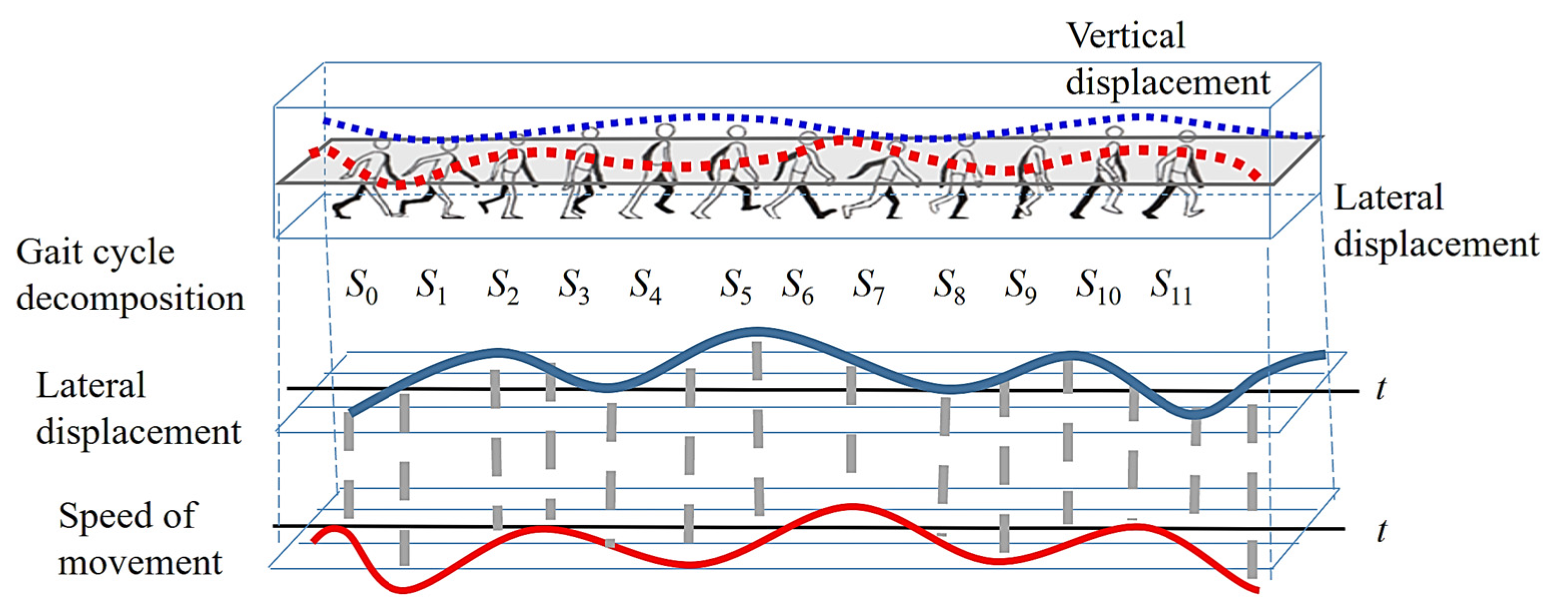
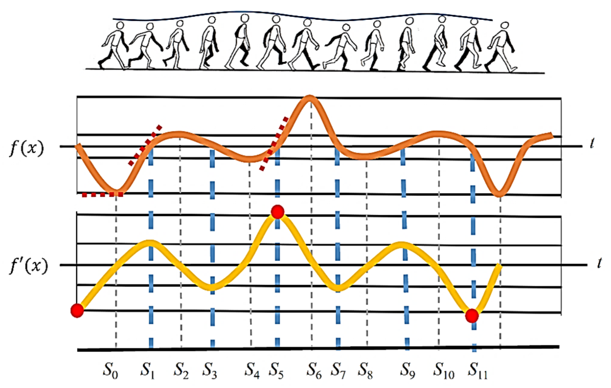
Since this paper uses the image displacement of first-person vision images for gait analysis, the decomposition of each gait cycle is based on the direction of motion. As shown in Figure 2, a gait cycle is divided into 12 movements. To subdivide each movement, it is numbered from S0 to S11. When the right foot is stepped down to touch the ground (right heel to the ground, IC), it is numbered as S0. After touching the ground, the body continues to squat down (LR), and the COG (center of gravity) is shifted to the center. Now the body is at its lowest point, and this movement is numbered S1. When the left foot is lifted off the ground (acceleration phase of the left foot), the COG of the body is moving to the left due to the force exerted by the left foot. Until the COG is about to become unbalanced, the COG of the body is at the far left, and this movement is numbered S2.
Figure 2.
Diagram of the decomposition of the direction of the body’s center of gravity.
When the body is about to lose its balance, the right foot pulls the body back to the center. Until the right foot is raised parallel to the left foot, the phase of middle of standing (MST) is presented. Now the COG of the body is shifted to the center, which is numbered S3. After that, the left foot continues to move forward (Deceleration Period, TSW), and due to the inertia theorem, the body continues to move to the right. Until the right foot supports the body, the weight of the body shifts to the far right, which is numbered S4. When the right foot is about to lose support to the body, the left foot is straightened forward (TSW). Then the COG is pulled back to the center point, which is called S5. At the next movement, the left foot is tilted to the lower left (left heel to the ground, IC), and the COG of the body is at the leftmost part, which is called S6. After this, the body begins to squat to the lowest point during gait, and the COG is downward and toward the center, which is called S7. When the right foot begins to lift off the ground (the acceleration phase of the right foot), and the body is about to lose balance, the body is inclined to the right, which is called S8. To regain balance, the left foot exerts force to bring the body’s weight leftward to the center. When the right foot is horizontal with the left foot, this is called midstance (MST) and is numbered S9. After that, the right foot continues to swing forward (right foot deceleration period), and the body continues to shift to the left due to the inertia theorem. When the left foot stands on tiptoe until the body is about to lose its balance, the COG of the body shifts to the far left, which is numbered S10. When the body is about to lose its balance, the right foot is straightened to pull the body back to balance and move the COG to the center point, which is called S11. Finally, the right foot continues to step down until the right heel hits the ground. Now the COG is far to the right, and the movement returns to S0, in which a new stride starts. To better understand the detailed movements of a gait cycle, the movements from S0 to S11 are organized into Table 1.
Table 1.
The movement decomposition of a gait cycle.
2.2. Relationship Between the COG of the Body and the Image Motion
When a clip-on video recorder is used as a first-person camera, the camera also shakes as the body sways vertically and horizontally. This effect results in blurred images recorded by the camera during the rapid displacement period. However, when the COG of the body is moved in a different direction due to the need for balance, it is necessary to slow down the movement speed along the current direction to stop. Therefore, there is a very short period during which the body is static, and the images have high clarity at this time. On the other hand, when the body is moving, the camera is also in motion, which causes the images to be blurred. Hence, the evaluation of image clarity can determine the time instants (S0 to S11) and movement directions in the gait cycle.
Through the trajectory of horizontal and lateral displacement, the movement speed of the body can be calculated from the slope magnitude. As the slope of the trajectory increases, the body is moving faster. When the lateral displacement of the body is at the far left and right, the velocity first approaches zero due to the change in body direction. At the same time, the slope of the lateral displacement trajectory also approaches zero. During the movement, the COM has continuous motion through the center point, and the slope of the trajectory is the largest. As shown in Figure 3, the odd-numbered feature points are all exactly the zero-cross points, and the even-numbered feature points are the extreme points along the direction of body motion. For all the odd-numbered points, it can be found that, during the process from S0 to S2 and S4 to S6, the moving direction of the body is larger. Therefore, the trajectory slope of the zero-crossing points in between them is larger than that of the other zero-crossing points.
Figure 3.
Direction of motion vs. velocity plot.
Through this data analysis, the optical flow method [29] is adopted in this paper to analyze the speed and direction of the movement of the feature points in the process of image motion. With the direction of walking, the greater the slope of the body’s displacement trajectory, the stronger the intensity of the optical flow. As a result, the moving direction of the body when walking can be derived corresponding to the time instant of a gait cycle. Therefore, by simply inputting the first-person vision images recorded from the camera worn by the test subject, the moving direction of the body when walking can be obtained. Finally, the gait features of each person can be determined through the different gait patterns of every individual.
3. Proposed Scheme
The gait parameters extracted using first-person vision images can be divided into three categories: temporal descriptors, spatial features, and kinematic features. After extracting temporal gait descriptors from images, the major approaches for evaluating image clarity include edge and high-frequency signal intensity measurements [30]. However, these methods are based on the number of edges inside the image; they are related to the image content but not to the movement of the image. To tackle this problem, this paper adopts the optical flow of pixels [31] as the descriptors, which have the advantage of being less dependent on the image content. When the test subject is in motion, the motion vector of each pixel calculated by the optical flow is larger, and this means that the image is in a blurred state at this time. Also, the opposite direction of the motion vector reflects the direction of human movement. Conversely, when most optical flow values are close to zero, the image is in a stationary state.
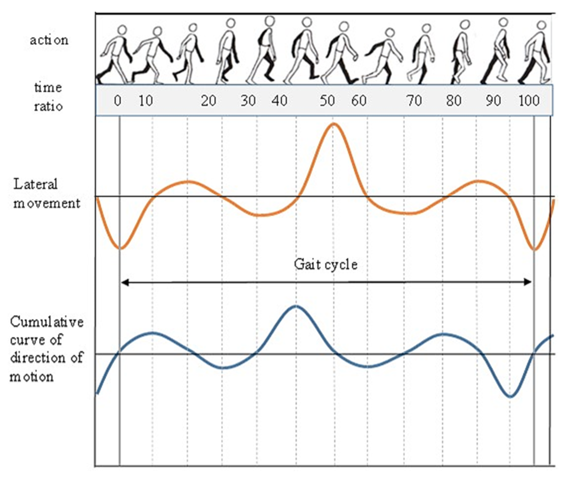
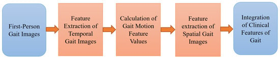
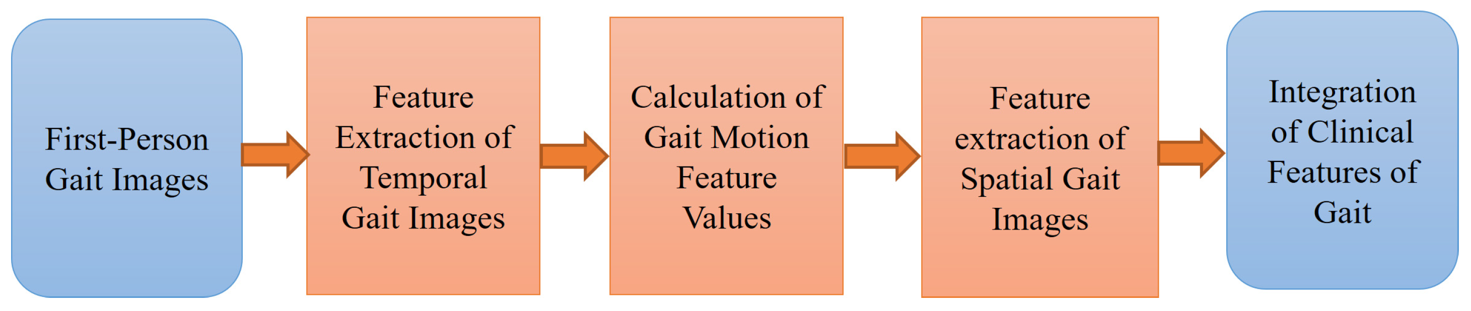
As shown in Figure 4, after the lateral displacement of the body over time is expressed as a displacement function, the cumulative statistics of the pixel motion vectors calculated from optical flow are proportional to the derivative function of the displacement function. The cumulative statistical characteristics of pixel motion vectors are regular, and there is stability in the specific feature occurrence position. Therefore, the corresponding feature values of gait motion in the statistical curve of motion vectors can be extracted through feature extraction. After feature extraction, the time instant corresponding to the time feature value can be used as the basis for extracting the spatial feature value in the image. Using the camera correction technique from computer vision, the feature values of spatial gait images can be calculated. Furthermore, after integrating the temporal and spatial feature values, the individual gait feature values and appearance can be fully represented. The processing flowchart is shown in Figure 5, which is described in the following sections.
Figure 4.
Graph of the optical flow statistics versus lateral displacement.
Figure 5.
Flowchart of feature extraction, analysis, and integration.
3.1. Feature Extraction of Temporal Gait Descriptors
Using the optical flow method [29], the vertical and horizontal components of vx and vy of the motion vector of each pixel in the image can be obtained. These two motion components of each pixel are used directly to calculate the average motion vector of the entire image, given by
In which the image size is m × n. vx(i) and vy(i) represent the motion vector components of the i-th pixel along the X and Y directions.
When the human body walks forward, the forward movement of the first-person camera causes the image content to expand and move to both sides. Since the length, angle, and direction of the pixel displacement vector in the image are different from those of a traditional third-person image, alternative methods must be used when analyzing the image content. According to the imaging model of the image, when the camera moves forward, the motion vector of a pixel in the image plane spreads outward relative to the image center.
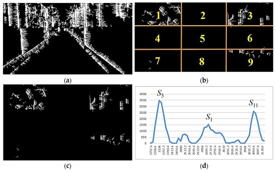
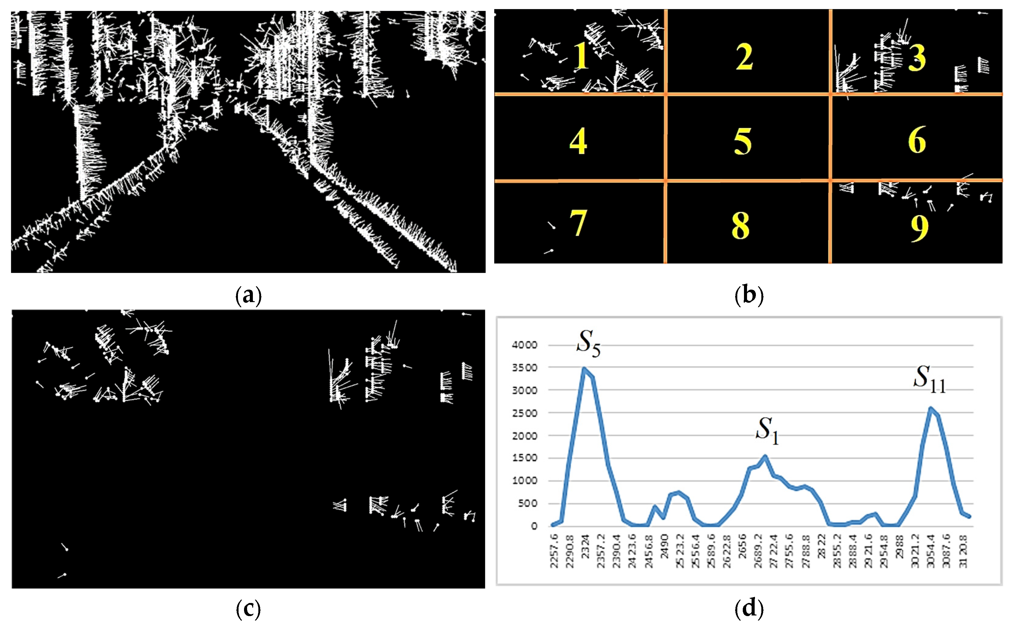
Because the motion vector has the factor of center spreading outward and the direction of vector movement is stable, it is expected that stable motion vectors can be obtained if only the longer motion vectors on the outside of the image are considered and the smaller motion vectors concentrated in the center of the image are filtered out. However, experimental results show that although the motion vectors have been filtered, there are still many motion directions in the whole graph that are misjudged due to noise. To tackle this problem, as shown in Figure 6b, we divide the image into equal 3 × 3 regions and, for regions 1, 3, 7, and 9 only, add up the number of pixel motion vectors in those four regions that exceed the threshold. This cumulative sum value indicates that a greater increase in optical flow response corresponds to a large degree of pixel movement. The more pixels in an image, the more pronounced this phenomenon becomes.
Figure 6.
Processing and statistics of pixel motion vectors. (a) Results of optical flow computation, (b) optical flow consideration area, (c) optical flow filtering, (d) statistics of motion vectors for a single gait cycle.
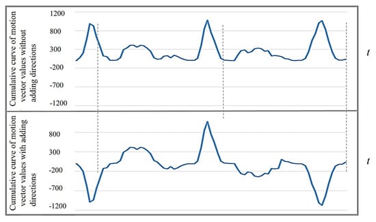
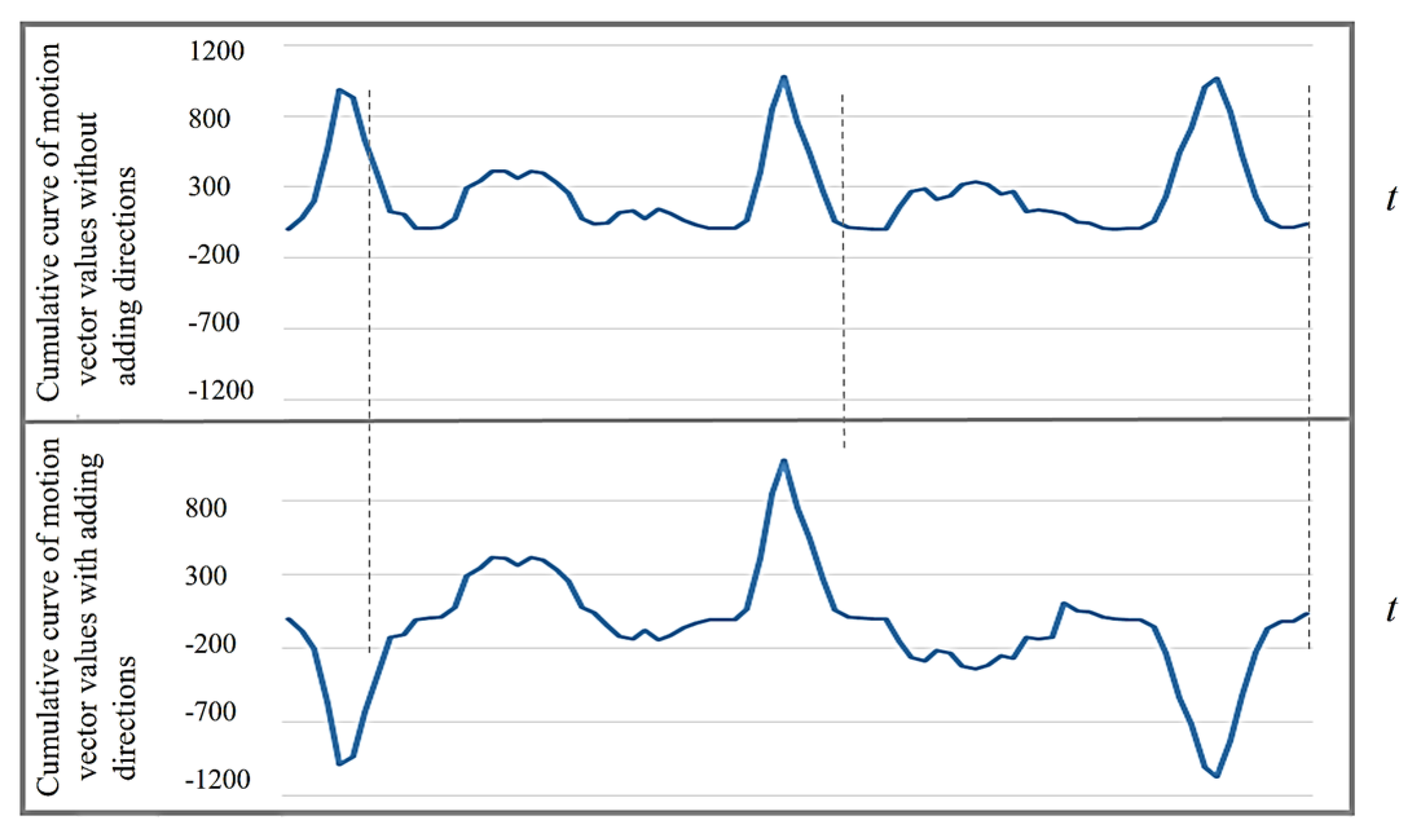
Therefore, corresponding to the lateral displacement in the cross-section of the human body, it can be found that since the horizontal displacement is the largest at time points S5 and S11 in a gait cycle, the number of pixel motion vectors in the four specific regions of the image is also relatively large. Furthermore, at the time points of S0, S2, S4, S6, S8, and S10, the number of motion vectors in a specific area of the image decreases due to the momentary static state. The direction of the current displacement of the body’s COG can be derived from the direction of the main pixel movement in these specific areas. For the sake of simplification, this paper only refers to the left and right directions of the motion vectors, and only vx(i) in Equation (1) needs to be referenced. In the image, assume that there are R motion vectors representing the body moving to the left (vx(i) > 0) and L moving to the right (vx(i) < 0). When R > L, the cumulative value of optical flow intensity a is set to a positive sign, which means that the body is currently moving to the left. If R < L, then a is set to a negative sign, which means that the body is moving to the right. After re-applying the positive and negative signs to the optical flow accumulation, as shown in Figure 7, the time points of S5 and S11 can be clearly distinguished, and each action time point in the gait can be further subdivided.
Figure 7.
Cumulative curve of motion vector values by considering the motion direction.
3.2. Calculation of Gait Motion Descriptor Values
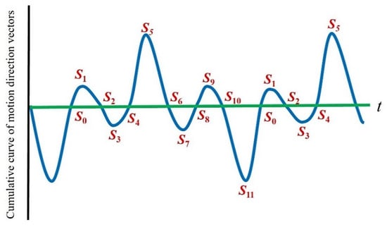
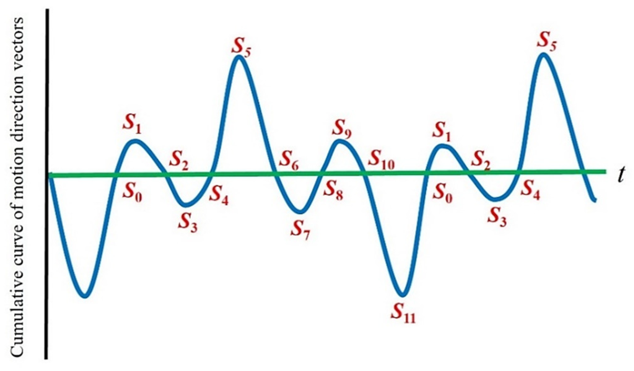
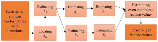
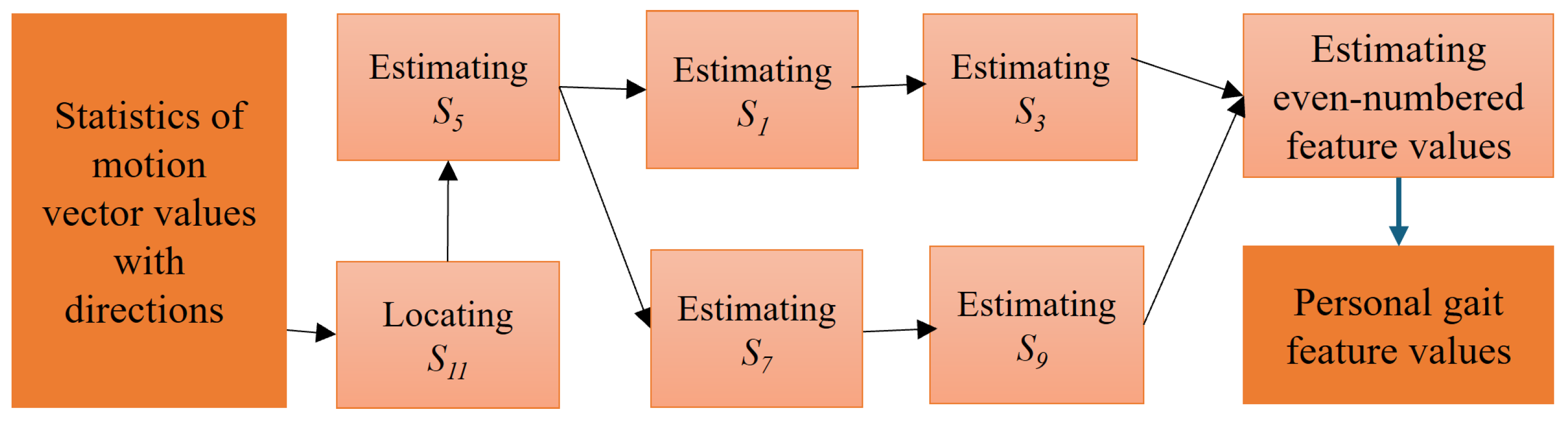
In the characteristic curve of the gait cycle, the time points S5 and S11 are the moments (ICs) before the left foot and the right foot swing and land on the ground, respectively. Also, the body belongs to the fastest-moving period in the gait cycle, and the statistical value of the motion vectors in the image is the most obvious and stable in the left and right directions. Therefore, the exact time points S5 and S11 can always be correctly obtained from the maximum values of each of the two directions, and there is also a stable cycle between adjacent steps. In this study, we used those two points as the anchors to further obtain other characteristic time points in the gait cycle. The complete time-position estimation model of descriptor values over a period of 5 gait cycles is shown in Figure 8.
Figure 8.
Positions of gait feature values.
The process of estimating the time points of gait descriptor values is shown in Figure 9, and the algorithm is described as follows:
Figure 9.
Process of extracting feature time points of motion vectors.
- [Input]: Cumulative function of motion vectors f(t), t = 1, …, N.
- [Output]: Cumulative function of motion vectors ti,j. The step number and the time descriptor number are represented by i and j, respectively.
- Step 1: Locating S11 = {ti,11}, i = 1, …, n.
Before looking for descriptor points, the first step is to search for the time point S11 where the right foot is in the IC period, and the body moves to the right side. Since several outliers exist inside the cumulative curve, to remove their influence, K-curvature is used to calculate the curvature and smooth the accumulation function of motion vectors. The value of each time point relates to the fourth point before and after itself, and the cosine value of its angle is calculated. The value of each time point relates to the fourth point before and after itself, and the cosine value of its angle is calculated by
When the value is closer to 0, it means that t is at the lowest point of a deep valley distribution at that time, and this point is regarded as the vertex of the curve. Furthermore, among all values with greater than 0.99, searching for the minimum value is to find the most stable descriptor of all S11 points. This descriptor is labeled as AS11.
Experimental results have demonstrated that each gait cycle of the user captured by the camera during the measurement is about 40~80 frames. Therefore, when AS11 is used as the benchmark to find the time descriptor point S11 of the adjacent steps on both sides, the search time range can be defined as [AS11 − 80, AS11 − 40] and [AS11 + 40, AS11 + 80]. This can locate the possible positions of the time descriptor point S11 in the previous step and the next step, respectively. After the minimum value of the motion vector accumulation in this range is obtained, the S11 of this step can be found. By following the same process, the S11 of each step in the whole walking process can be found, and the S11 of the i-th step is marked as ti,11.
- Step 2: Estimating S5 = {ti,5}, i = 1, …, n.
Relative to the standing period (IC) of the right foot landing support (S11), the left foot also has the standing period S5. For a normal gait, the time difference between S11 and S5 should be the same. Therefore, the method of obtaining a stable descriptor value S5 is to find the maximum value in the range of 1/3~2/3 between two S11s in the adjacent gait cycles.
- Step 3: Estimating S1 = {ti,1} and S3 = {ti,3}, i = 1, …, n.
When the body weight begins to fall on the right foot after the right foot is supported (S11), the right foot is flattened. Then the dorsiflexor muscles contract centrifugally in the opposite direction (left) to avoid the sole of the foot hitting the ground. This time point is defined as S1. This is followed by the middle period (IC) of the right foot, and the forward swing of the left foot forms a rightward shift in the COG, which is defined as S3. Therefore, S1 and S3 are located between S11 and S5 in the continuous gait and correspond to the maximum and minimum values in this period.
- Step 4: Estimating S7 = {ti,7} and S9 = {ti,9}, i = 1, …, n.
When the body weight begins to fall on the left foot after the left foot is supported (S5), the left foot is flattened. Then the dorsiflexor muscles contract centrifugally in the opposite direction (right) to avoid the sole of the foot hitting the ground. This time point is defined as S7. This is followed by the middle period (IC) of the left foot, and the forward swing of the right foot forms a leftward shift in the COG, which is defined as S9. Therefore, S7 and S9 are located between S5 and S11 in the continuous gait and correspond to the maximum and minimum values in this period.
- Step 5: Estimating the even-numbered gait descriptor values.
The even-numbered time point set in this paper is the zero-crossing point between the adjacent odd-numbered time points mentioned above. This represents the stationary time point when the body’s COG changes the direction of displacement. Since the length of the stationary time of every individual is affected by the ability to control muscle strength and nerves, the length could be different. Therefore, there may be multiple unstable zero-crossing points for a long time between adjacent odd-numbered points. To solve this problem, the time center of adjacent odd-numbered points is used as the benchmark, and the closest zero-crossing point is set as the even time point.
3.3. Feature Extraction of Spatial Gait Images
In this paper, the walking video is recorded from a first-person perspective, and the checkerboard squares are used as the image content. The relationship between distance and rotation can be obtained by comparing the size or rotation degree of the image content to their actual values in the real world. This can provide the distance between the camera and the image and the angle of the camera’s rotation. Using the images captured from the camera coinciding with body shaking, the personal gait parameters, such as step length, step width, and body rotation, are calculated. However, the requirement for a reference object still introduces an environmental constraint for spatial-parameter estimation. The advantage of the proposed configuration is not that spatial calibration requires no external setup, but that the camera moves with the subject and consequently does not require multiple externally positioned cameras covering the entire walking path.
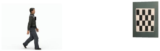
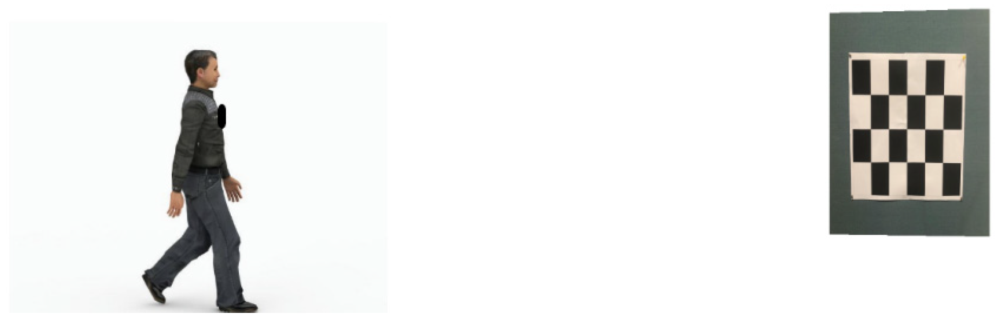
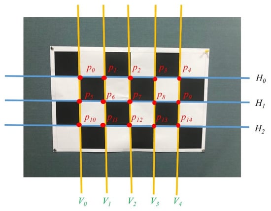
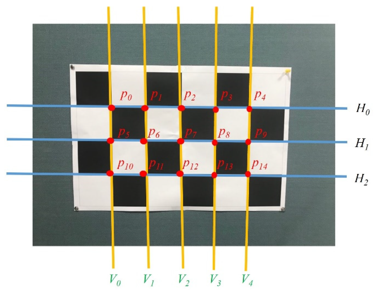
The environment of feature extraction for spatial gait images is shown in Figure 10. A checkerboard of 6 × 4 with a grid length of 120 mm is used to define the World Coordinate System (WCS). The positions of the checkerboard squares in the image and the coordinates of the corner points of each box on the checkerboard can be obtained, as shown in Figure 11. A total of 15 corner points, , k = 0, …, 14, in the inner boxes can be found in the checkerboard squares.
Figure 10.
The environment of feature extraction for spatial gait images.
Figure 11.
Schematic diagram of the position of the corner points of the checkerboard.
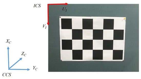
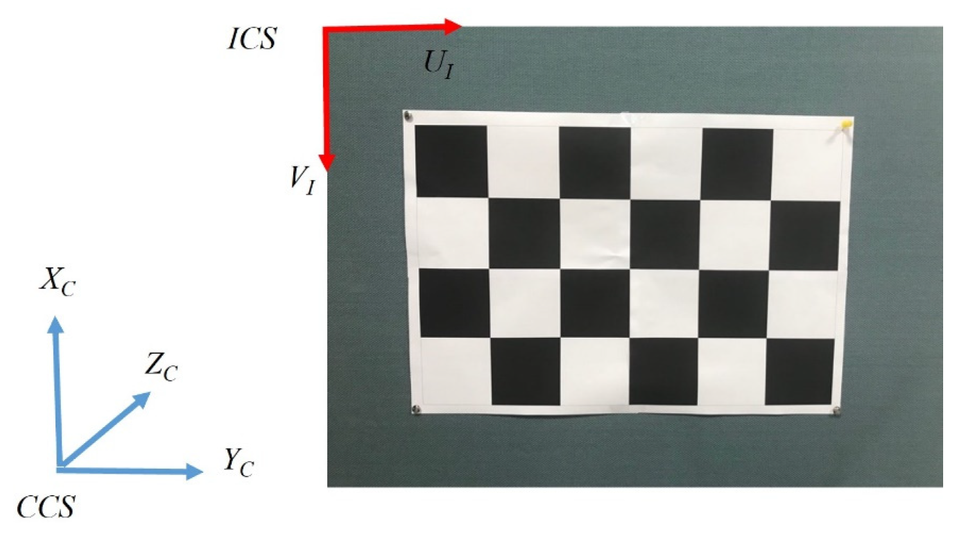
Since the origin of the Image Coordinate System (ICS) is set in the upper left corner of the image plane, the UI axis is positive to the right, and the VI axis is positive downward. This is different from the setting of the Camera Coordinate System (CCS), in which the XC axis is positive upward, and the YC axis is positive to the right (as shown in Figure 12). Therefore, it is necessary to convert the coordinate axis direction of the ICS to be consistent with the CCS. That is, the UI axis is parallel to the XC axis, and the VI axis is parallel to the YC axis. For the W × H image, the new checkerboard corner coordinates are
Figure 12.
Camera Coordinate System and Image Coordinate System.
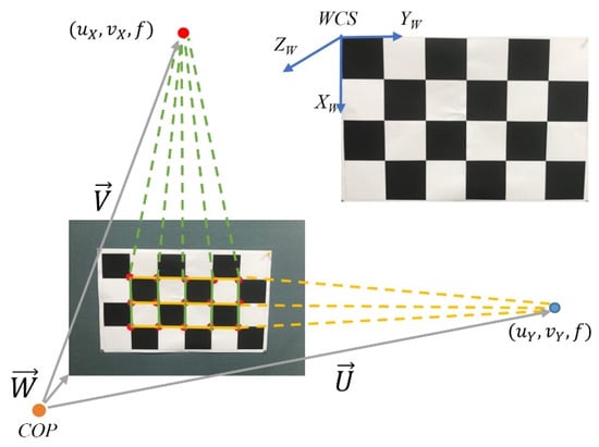
To estimate the relationship between WCS and CCS, we assume that the directions of the three axes are (1, 0, 0)W for XW, (0, 1, 0)W for YW, and (0, 0, 1)W for ZW in the world coordinate system, as shown in Figure 13. In the image, a checkerboard of 6 × 4 (or 15 corner points inside the inner checkerboard boxes) can be imaged to define five vertical straight lines. According to the vanishing point principle, the center point of the CCS, COP, and the indefinite extended intersection of the five perpendicular lines will form a ray that is parallel to XW. Therefore, when the checkerboard corner points pi, pi+5, and pi+10 on the image are connected into a line Vi, i = 0, …, 4, a total of 5 lines can be achieved. Theoretically, their infinite extensions can intersect at the vanishing point (uX, vX). Since each line is made up of three checkerboard corner points, it can be represented as follows by a matrix-vector:
Figure 13.
The transformation relationship of CCS and WCS.
After pseudo-inverse computation, we can obtain ai and bi, where i = 0, …, 4. Then the equation for each straight line Vi can be calculated. Let the grid edge line VLi on the checkerboard be imaged as Vi and parallel to XW. The equation of VLi can be represented as
where [kxi, kyi, kzi]T is any point along VLi represented by CCS coordinates. [Xx, Xy, Xz]T is the direction vector of the straight line VLi, which is the direction vector representation of XW in CCS. In the CCS, the perspective projection relationship can be expressed as
Therefore, the following formula can be obtained:
(f ⋅ gXi)Xx − (f ⋅ dXi)Xy − (cXigXi − dXieXi)Xz = 0
By substituting (5) into (4), the equation is given by
aieXi + bigXi = 0
Hence, the results become ai = gXi and bi = −eXi.
Assume that cXi and dXi are the average values of the imaging points on each imaging line. nX = [Xx, Xy, Xz]T is the common direction vector of each straight line VLi corresponding to XW. For i = 0~4, a homogeneous simultaneous equation can be obtained as follows:
The homogeneous simultaneous equation can be expressed as AnX = 0, but there exists a meaningless solution, . To avoid this, a restriction condition is required. Therefore, the solution problem is transformed into an optimization problem.
The method of Singular Value Decomposition (SVD) is adopted in this paper to solve this optimization problem. The column vector in the orthogonal matrices corresponding to the minimum value is the optimized nX solution and the representation of XW in CCS. Similarly, the representation of the horizontal YW in CCS can also be obtained in the same way by three horizontal imaging lines and labeled as nY. Since WCS is a Cartesian coordinate system, when the unit direction vectors of XW and YW in CCS are known, the ZW direction vector can be obtained by the outer product:
and set .
The transformation relationship between CCS and WCS can be defined by a rotation matrix R and the displacement vector T, written as
The displacement vector T is the vector from COPCCS to COPWCS.
3.4. Integration of Clinical Features of Gait
Each person has different gait characteristics due to factors such as body size, physical health status, age, and gender. Through the above extracted feature values, a multi-dimensional representation of individual gait features can be constructed, which includes the feature values generated from each step and taking the average across all individual gait cycles. For the test subject numbered k, the j-th time feature point calculated in the i-th step is denoted as tk,i,j (unit ms), and the corresponding statistical value of optical flow is a′k,i,j. Since the number of optical flow vectors is different under distinct measurement scenarios, each a′k,i,j is re-quantized using a′k,i,11 as the benchmark (corresponding to S11 of the i-th step):
such that all ak,i,11 = 1. In the time domain, the most primitive information is tk,i,j. The time used for the i-th step is
dk,i = tk,i+1,0 − tk,i,0
Because there are subtle differences between gaits, traditionally, each time feature point in the gait cycle is based on the gait cycle, and the time feature is quantified as a percentage by
When the gait features of the subject are captured, because the space-related features need to be imaged by using checkerboard squares, they need to have clear and non-wobble images. Therefore, only the instantaneous images numbered as even-numbered time feature points will be processed, and the displacement vector Tk,i,j = [TXk,i,j, TYk,i,j, TZk,i,j]T between the camera (human body COM) and the checkerboard squares at the corresponding time points will be obtained.
After re-quantizing the above feature values, we can represent the i-th gait feature of the k-th test subject as a feature vector, which includes
- (1)
- Normalized feature values: Ak,i = [ak,i,1, ak,i,3, ak,i,5, ak,i,7, ak,i,9];
- (2)
- Time feature point: Pk,i = [Ptk,i,1, Ptk,i,2, …, Ptk,i,10];
- (3)
- Time duration of each gait cycle: dk,i;
- (4)
- Spatial gait features: Tk,i = [Tk,i,0, Tk,i,2, Tk,i,4, Tk,i,6, Tk,i,8, Tk,i,10].
Therefore, there are 34 values in the gait feature vector of the i-th step of the k-th test subject, which are organized as follows:
The overall average representation of gait features for the n steps of the k-th test subject is defined as
In clinical practice, the traditional time parameters used include stride frequency (steps/min), left/right step length (cm), gait cycle (sec), stride (cm), step speed (cm/sec), step deviation (cm), double support phase (%), left/right lower limb support phase (%), and left/right lower limb swing phase (%). Depending on the sampling rate of the camera (the current system is 60 Hz), the temporal gait parameters can be calculated as follows:
- (1)
- Stride Frequency (steps/min): In a valid gait video with nf frames including n steps (or counting the number of S5), the stride frequency is defined by
- (2)
- Gait Cycle (sec): In a video containing nf valid gaits, the number of S5 is calculated and converted to time units in seconds, so that the gait cycle is defined by
- (3)
- Double Support Phase (%): This refers to the average of the sum of phases occupied by the feature points of S0 to S1 and S6 to S7 in each step.
- (4)
- Right/Left Lower Limb Support Phase (%): This refers to the phase average of the feature points from S0 to S7 of the right lower limb support phase and from S6 of the left lower limb support phase to S1 of the next step in each gait cycle.
- (5)
- Right/Left Lower Limb Swing Phase (%): This refers to the phase average of the feature points from S1 to S6 of the left lower limb swing period and the feature point S7 of the right lower limb swing period to the end of the current step in each gait cycle.
On the other hand, the spatial gait parameters can be computed as follows:
- (1)
- Left Step length (mm): This refers to the distance of body movement that the left foot moves from the ground to the time it touches the ground.
- (2)
- Right Step length (mm): This refers to the distance of body movement that the right foot moves from the ground to the time it touches the ground.
- (3)
- Step Difference (mm): The difference between left and right step length
Dk = |LLK − LRk|
- (4)
- Step Speed (mm/s): The time spent on each step
4. Experimental Results and Evaluation
4.1. Setup of Experimental Environment
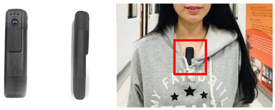
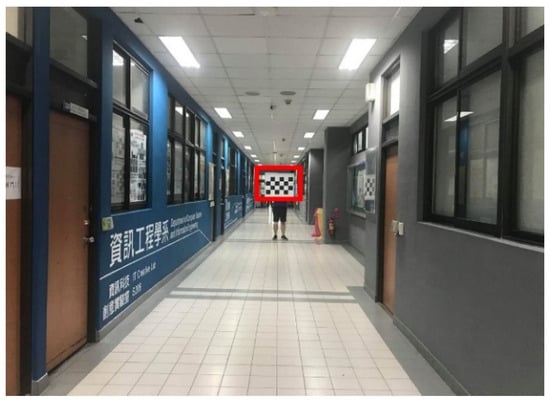
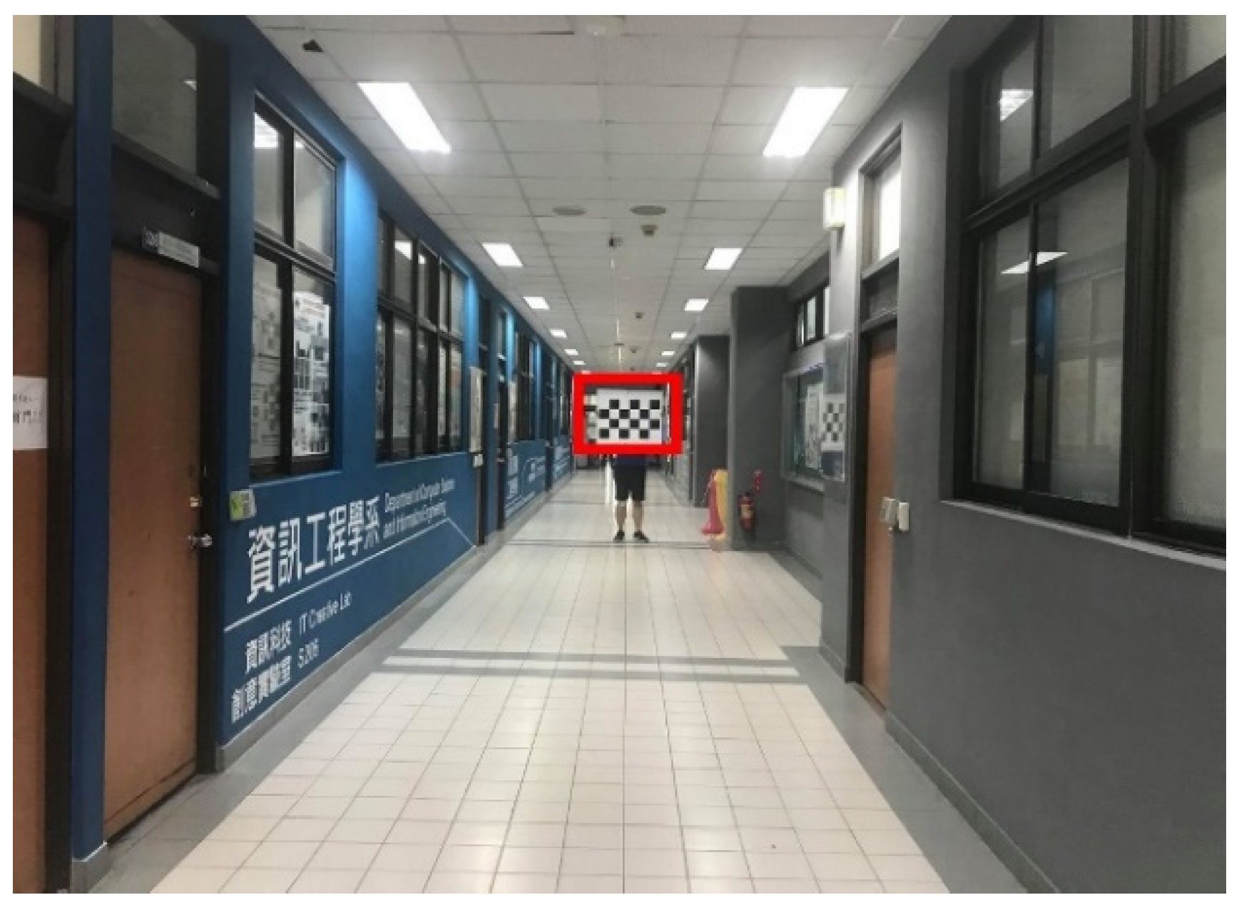
The approach developed in this paper is to use a wearable 60 fps camera (a cipher recorder) that can be mounted on the chest, and the start button can be pressed to record the walking posture (as shown in Figure 14). When the video recording was completed, the gait analysis and parameter computation could be automatically finished by simply moving the images to the designed system. In this study, the temporal and spatial gait parameters were analyzed. The temporal gait patterns could be measured anytime and anywhere because only the flow direction of the image is considered. To include the measurement of spatial gait parameters, a reference basis with absolute length (e.g., a checkerboard) needs to be added. Considering the size of the checkerboard squares, the spatial gait parameters can be accurately calculated by placing a checkerboard image with a length of 12 cm, a width of 12 cm, and a grid of 6 × 4 squares at the end of a 20 m-long walkway, as shown in Figure 15. Therefore, in a medical institution, a fixed checkerboard image can be placed on the wall at the end of the corridor of the ward, consultation room, or the home environment. Note that the experiment is done along the corridor in front of classrooms.
Figure 14.
Clip-on camera and usage.
Figure 15.
The recording environment for spatial gait parameters.
4.2. Performance Comparison Between Motion Capture System and First-Person Camera
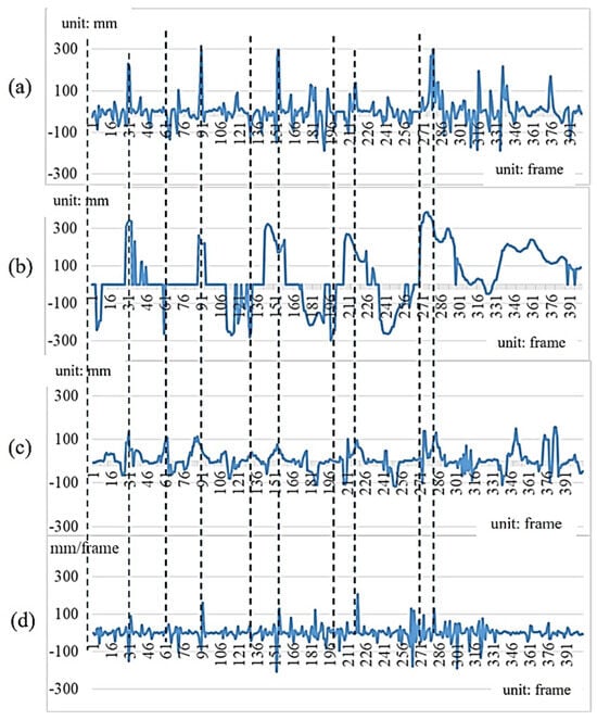
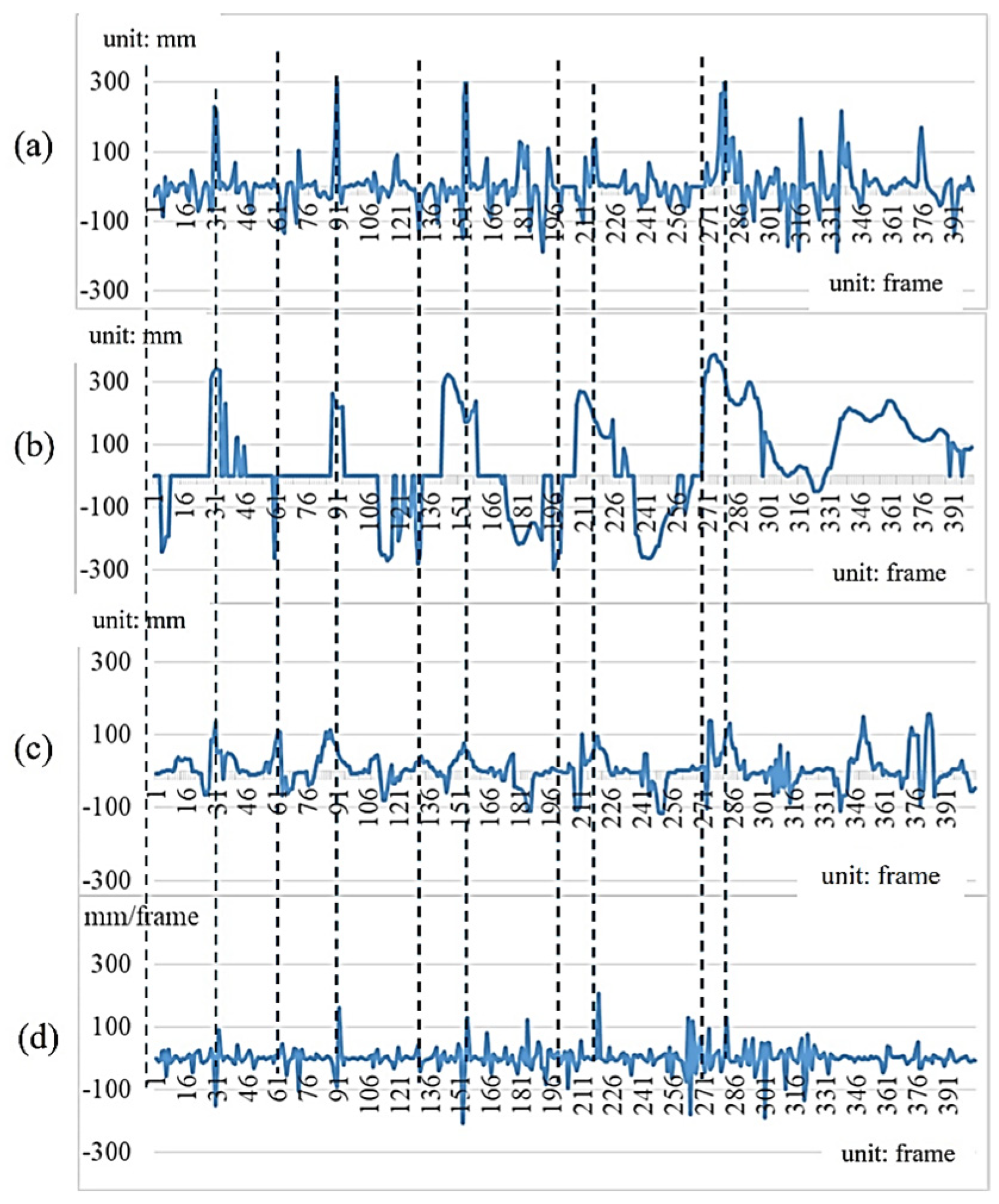
The motion capture system used in this experiment is a 3D Suit®, which can detect 17 body positions simultaneously in the 3D space and capture up to 2000 frames per second. To match the first-person camera, a sampling rate of 60 fps is adopted. This experiment is treated as the reference-system comparison. Based on gait measurement for the same subject walking six strides with 426 frames, Figure 16a and Figure 16b show the depth values of the Spine point obtained from the motion capture system and the spatial feature values of gait images from the first-person camera, respectively. These are the values of the Y-axis coordinates in the 3D coordinate space. Figure 16c is obtained from the first-person camera and represents the cumulative motion-vector values derived from the image sequence. Figure 16d, in contrast, is derived from the motion capture system by differentiating the Y-coordinate trajectory shown in Figure 16a, and therefore represents the reference motion-velocity signal. Compared with the statistics of motion vectors obtained from the first-person camera, it can be regarded as the equivalent feature values.
Figure 16.
Comparison of data captured from a motion capture system and a first-person camera: (a) Y depth values of the Spine point from the motion capture system; (b) spatial values of the first-person camera; (c) Accumulated motion vectors of the first-person camera; (d) motion-capture-derived velocity values.
As shown in Table 2, the difference values of gait parameters obtained from the motion capture system and the first-person camera are small. The approach using the first-person camera has demonstrated the performance of high accuracy, and the error rates using the curve of temporal gait descriptor values are 0.064 and 0.074, respectively. Note that the values in Table 2 are not the total recording duration. They represent the average temporal interval associated with the left-foot and right-foot steps, respectively, expressed in milliseconds. Small differences between the two measurement approaches arise from the independently detected gait-event timing in the motion capture and first-person image signals.
Table 2.
Quantitative comparison of the results obtained from a motion capture system and a first-person camera.
4.3. Short-Term Repeatability of the Extracted Gait Features
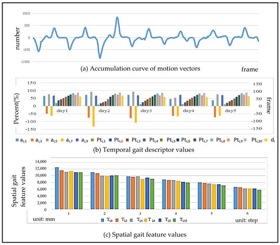
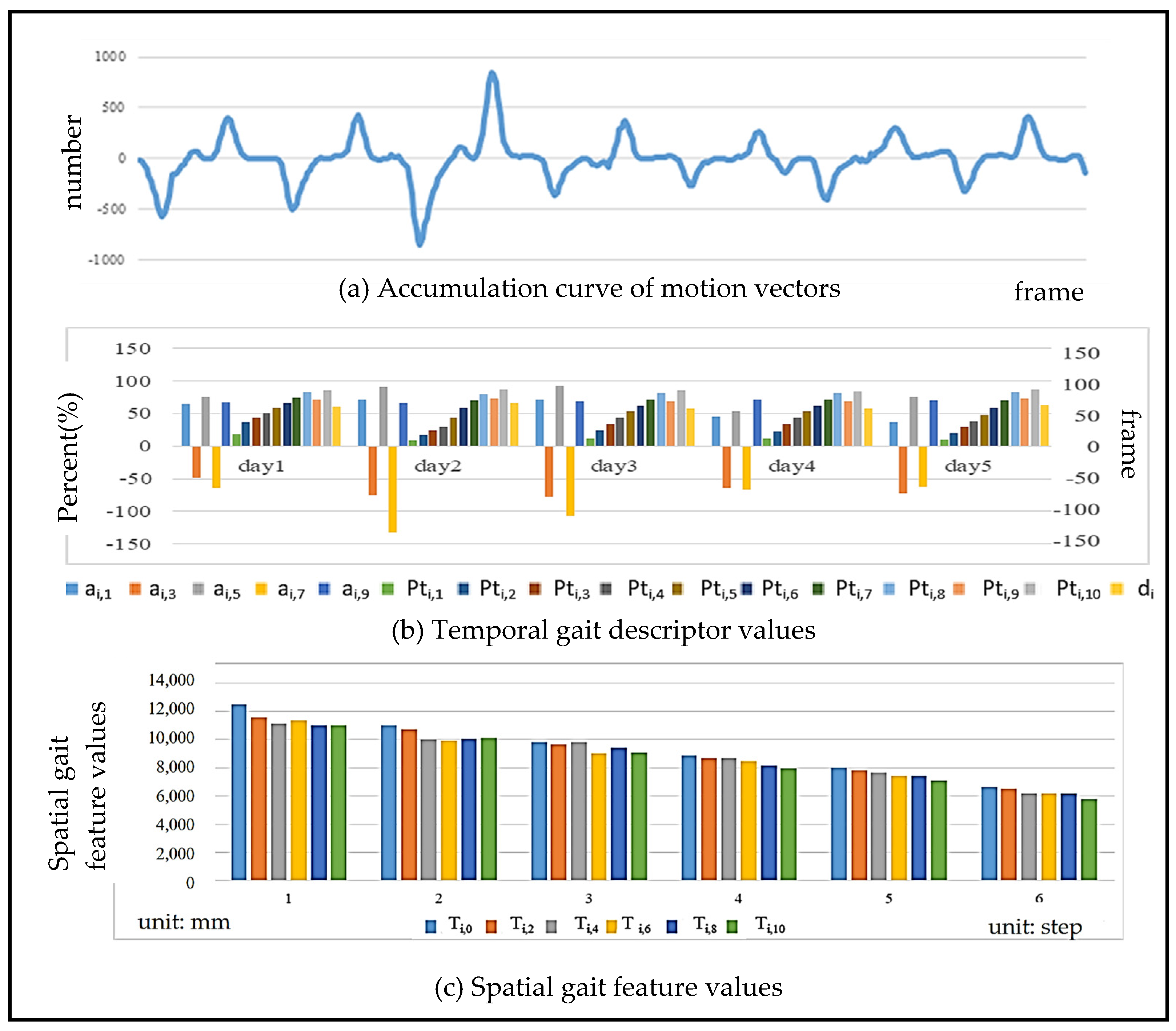
Walking is a regular and steady movement, so the gait results analyzed with a first-person camera must conform to this requirement. Figure 17 shows the gait results of the same person walking six strides with 426 frames in a row using the proposed approach in this paper. Since the maximum and minimum peaks of consistency and regularity can be seen in the accumulation curve of motion vectors in Figure 17a, the repeatability of the gait during walking is demonstrated. The y-axis represents the number of motion vectors counted at the time instant of each frame. In the gait cycle, the movements corresponding to the maximum and minimum peaks are the process of stepping rightward or leftward to the ground. The body is moving quickly to the right or left due to the leg lifting, and the speed is the fastest period in the entire gait cycle. The results of the calculated temporal and spatial gait features are shown in Figure 17b and Figure 17c, respectively. The temporal gait descriptors contain the odd feature points ai,1~9 in the accumulation curve of the motion vector, the time ratio Pti,1~10 of each feature point, and the time d of each stride. The spatial gait features include the spatial depth value of each feature point with an even number, showing a steady decreasing trend, representing the gradual approach of the body to WCS. Note that the overall test consists of a total of 6 strides and a division of 426 frames.
Figure 17.
The gait results analyzed for the same person walking six strides with 426 frames.
Also, we have collected the gait feature values of the same person after walking about 60 strides per day for five consecutive days. Table 3 shows the difference results of individual gait descriptors, demonstrating the quantitative results of the normalized feature values and temporal feature points of the i-th person. It can be found that between each gait, the difference between most of the values is small, except for the feature points ai,5, because the corresponding movement of the body swing is relatively large, so the difference between the values is also large. Table 4 shows the results of the average squared difference between the gait descriptor values on each day (d1~d5). The average value is 2468, which is much smaller than that of different people shown in Table 5 (the average value is 7743). In the following sections (Section 4.4, Section 4.5 and Section 4.6), the main purposes of all experiments focus on exploratory characterization of the extracted gait descriptors, rather than ground-truth validation.
Table 3.
Quantitative results of individual temporal gait descriptors calculated from the box plot.
Table 4.
Quantification of differences in individual temporal gait descriptor values.
Table 5.
Difference scale of temporal gait descriptor values between different genders.
4.4. Gait Difference in Different Individuals
Although walking is a daily exercise, walking habits cause changes in gait characteristics. Table 6 shows the numerical results of temporal gait descriptor values in the box plot among 10 people. Since the values in the IQR are larger than those in Table 3, this demonstrates that the gait discrepancy among different people is large. Table 5 shows the mean squared difference in gait feature values between five males (b1–b5) and five females (g1–g5). There are a total of 10 people, and the average value is 7743. Compared with the average value of 2468 in Table 4, this shows that the temporal gait descriptor values between different people are quite diverse.
Table 6.
Quantitative difference results of temporal gait descriptor values between different people calculated from the box plot.
4.5. Gait Difference in Different Genders
Bohannon [32] mentioned that gait speed varies between genders and ages. Oberg et al. [33] claimed that men have less hip flexion and extension than women when walking, which is reflected in the fact that men have more body sway than women when walking. In this paper, five males (b1~b5) and five females (g1~g5) were tested with 60 steps to analyze the differences in gait feature values. The mean squared difference in the feature values between the ten participants is shown in Table 5, where the darker the green color, the greater the difference. From the color distribution, it can be found that there is more difference between different genders and less difference among the same sex in gait feature values. However, the gait differences between different genders are caused by the differences in individual walking habits and physical characteristics. Therefore, experimental results in this paper cannot be generalized to all men and women, and the differences in gait features between men and women are for reference only.
4.6. Gait Differences Among Different Age Groups
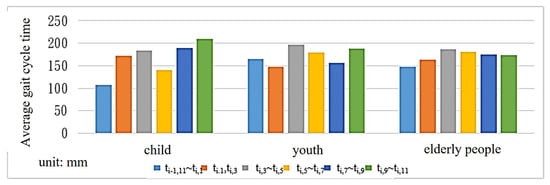
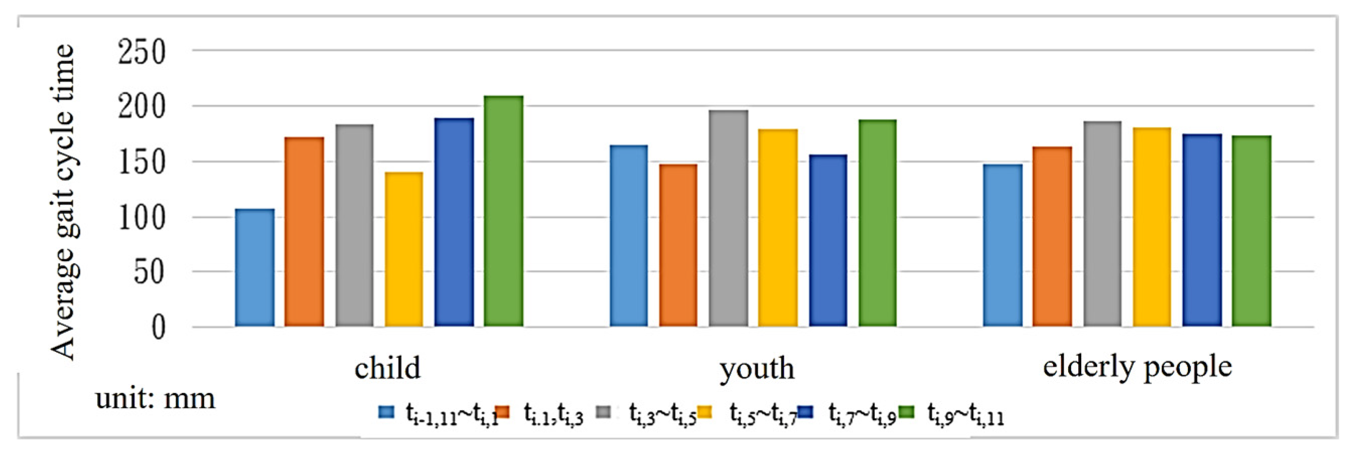
Gait characteristics vary among human age groups. Bohannon [32] proposed that older people tend to walk slower than younger people. According to the study, when the speed slows down by more than 0.1 s, the probability of cognitive impairment in the brain increases by 47%. In this paper, 10 people were selected from each of the three different age groups under 12 years old, 12~50 years old, and over 50 years old for gait analysis. As shown in Table 7, elderly people generate the longest gait cycle time among the three age groups. However, since most of the elderly people tested in this paper are under normal physical conditions and have not yet retired, the difference in gait cycle time compared with the two other groups is smaller.
Table 7.
Average gait cycle time among different age groups.
Figure 18 shows that the gait feature values of primary school students are different in S11~1, S1~3 and S3~5. Compared with the young and the elderly, the time spent on S3~5 (the heel off the ground (TST)) is shorter than that of S11~1 (the time of the heel to the ground (IC)).
Figure 18.
Average gait cycle time across age groups.
4.7. Performance Evaluation of Image Analysis
Using images as data sources for analysis, while featuring simple equipment and 2D sensing capabilities, also inherits many factors that affect imaging, which affects the robustness of image information. This section explores whether the analyzed temporal gait parameters remain unchanged when the image is subjected to camera tilt, different ambient lighting, or scene complexity, in order to demonstrate the robustness of the results.
- The Experiment of Camera Tilting
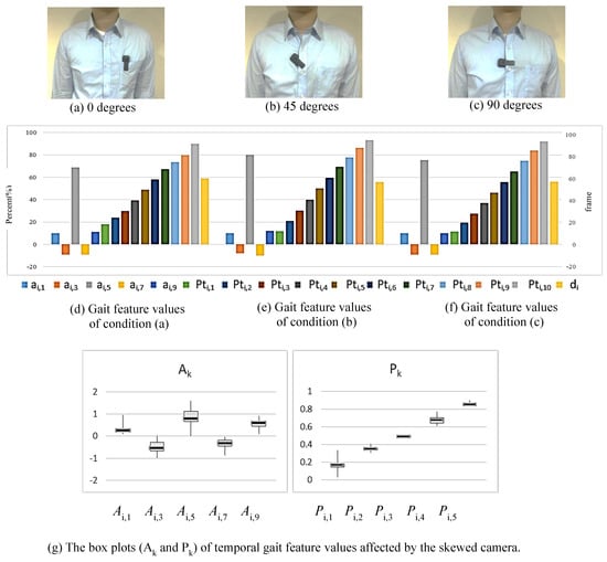
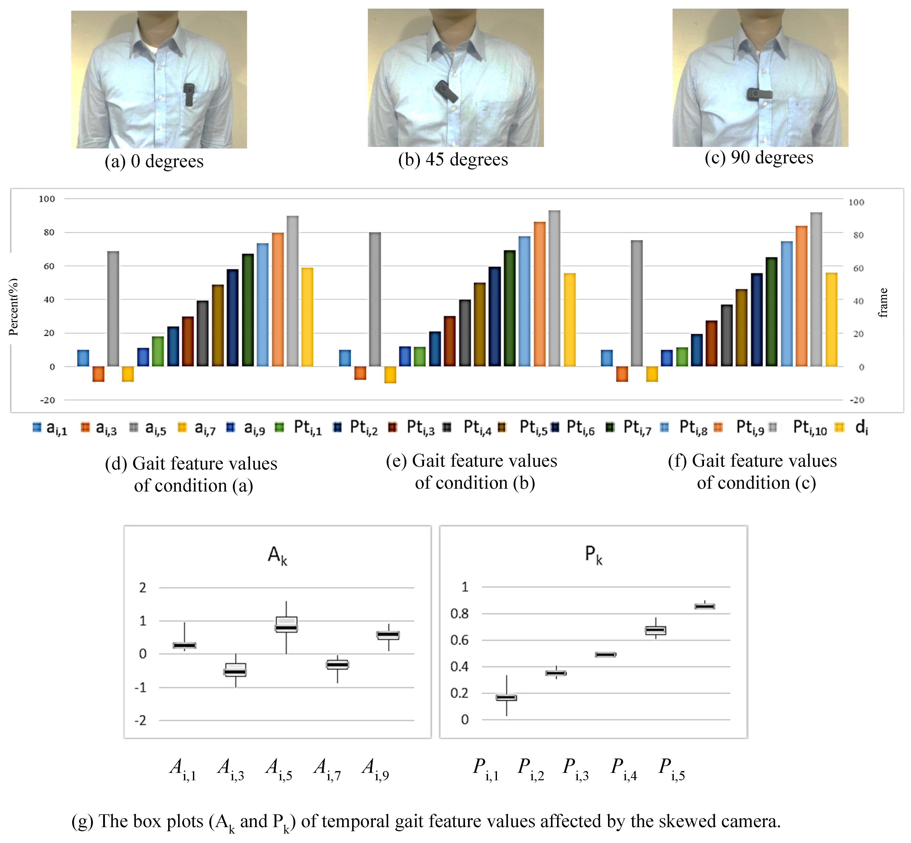
This system emphasizes that the person being observed can wear it themselves, without the need for professional assistance. Therefore, it can be used in non-medical institutions and in home environments. However, with such flexible wearing, the camera may become skewed. In this experiment, the camera is mounted in three conditions: (a) 0 degrees (vertical); (b) 45 degrees (skewed); (c) 90 degrees (horizontal), as shown in Figure 19a–c. In each condition, the test subject walks around 60 strides, and the corresponding gait feature values are collected and analyzed. Figure 19d–f show the representation of gait cycles computed from the temporal gait descriptor values corresponding to three conditions. As shown in the box plots of Figure 19g, the personal gait is shown to be stable and not affected by camera tilting. The box plots are made by combining the gait feature values from three conditions with different angles.
Figure 19.
The temporal gait feature discrepancy of the same person resulted from the skewed camera.
- The Experiment of Ambient Lighting
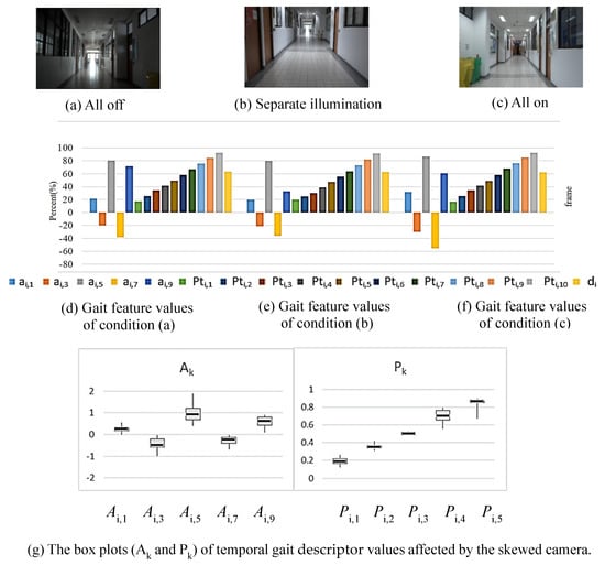
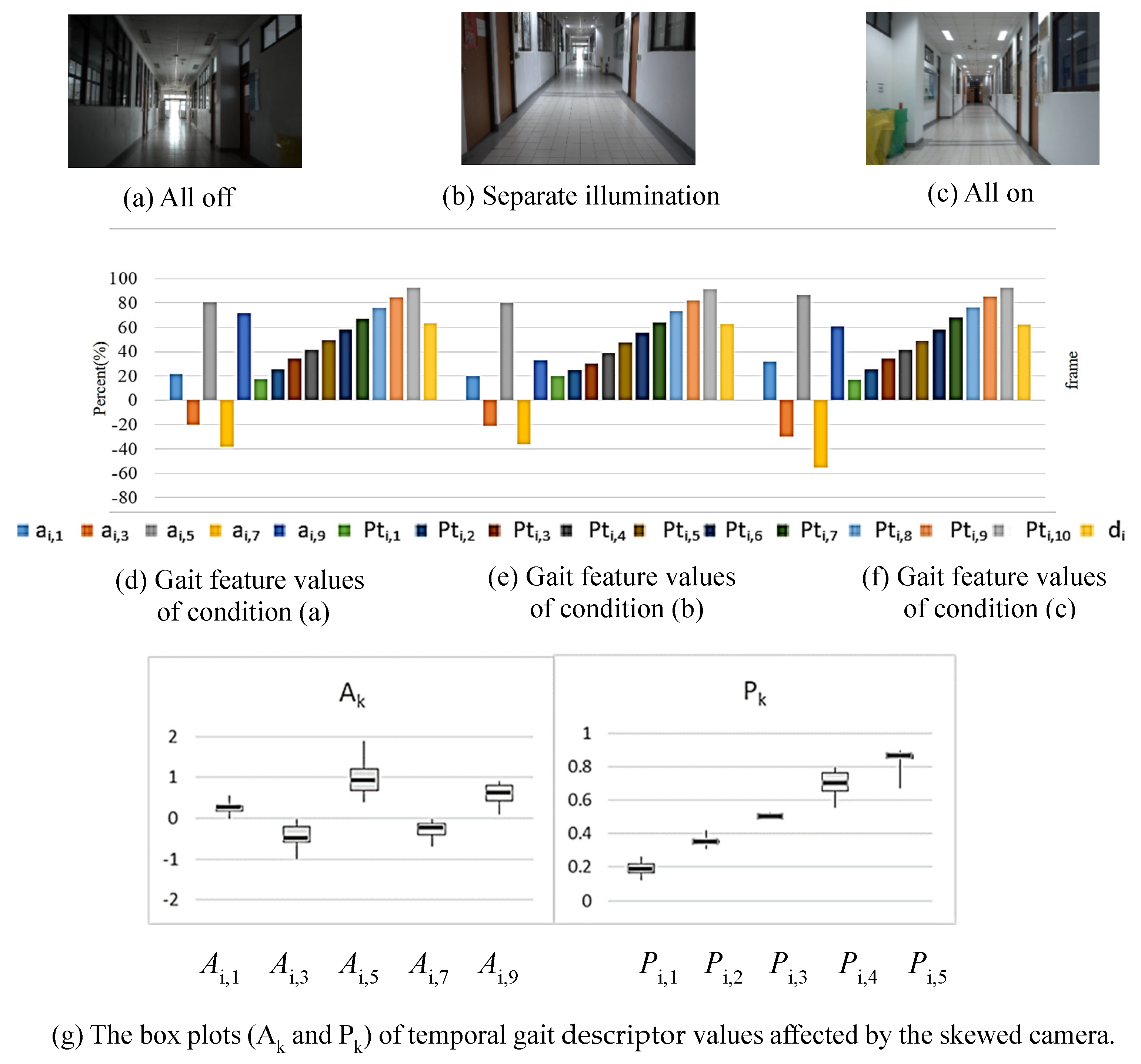
The intensity of ambient light sources is an important factor affecting the capture of image content. For longer gait detection, there are inevitably issues with light source intensity changes. To address this issue, this experiment sets the lighting to all off, separate illumination, and all on scenarios to check the system’s effectiveness (see Figure 20a–c). Figure 20d,e demonstrate the average values of feature points (around 60 strides) under three conditions of ambient lighting. As shown in the box plots of Figure 20g, the personal gait is shown to be stable and not affected by ambient lighting.
Figure 20.
The temporal gait descriptor analysis of the same person for different changes in ambient lighting.
5. Conclusions
Gait can demonstrate the motion characteristics of individuals and is used as a fundamental basis for assessing their physical conditions. Therefore, accurate gait analysis is an essential demand in clinical medicine. In this paper, a new approach to gait analysis is proposed by using a simple image recorder to capture images captured from a first-person perspective. The degree of sway in human walking can be deduced by analyzing image information from video. Since the camera follows the subject, there is no question of the scope of the test environment. Compared with the existing clinical medical methods, this approach is more suitable for use in the home environment. The proposed first-person configuration provides a less restrictive means of acquiring gait-related visual information and demonstrates the feasibility of extracting repeatable temporal and spatial gait descriptors from such recordings.
The acquisition and analysis of gait information use optical flow on the image pixels to obtain temporal gait parameters. By calculating the distance and rotation between the camera and the world coordinates, the spatial gait parameters are calculated by using the method of deriving 3D information from 2D images. In both cases, the analysis process does not require large and complex calculations. For every single individual, experimental results have shown to be conserved in gait parameters and remain robust in complex or dynamic environments. On the contrary, discriminability has been demonstrated between different individuals. Therefore, this approach can be further used for gait analysis to improve the quality of clinical medicine. This can also provide the advantage of convenience and suitability to apply for long-term healthcare at home.
Author Contributions
T.-L.C.: conceptualization, methodology, and supervision. C.-Y.C.: software and experiments, writing—original Chinese draft preparation. P.-S.H.: data curation, visualization, writing—review and editing. All authors have read and agreed to the published version of the manuscript.
Funding
This research received no external funding.
Institutional Review Board Statement
The study did not involve any clinical procedures, biomedical experimentation, or collection of sensitive personal data. In Taiwan, the regulations of the Institutional Review Board (IRB) are formulated by the Department of Medical Affairs, Ministry of Health and Welfare (MHW). According to the Human Subjects Research Act (29 articles) of MHW, our study belongs to the level of Exempt from Review, which is a low-risk research involving publicly available datasets, anonymous surveys, or non-invasive educational measurements. Our study, being observational, non-interventional, and of no risk, is exempt under this regulation. All experiments in this paper are non-invasive educational measurements. Nevertheless, we affirm that all procedures complied with the ethical standards of the 2013 revision of the Declaration of Helsinki, including respect for informed consent, privacy, and voluntary participation. Participants were informed of the study’s purpose and their right to withdraw at any time without consequence. No personal or identifiable information was recorded. The above is assumed to be an exemption from the ethical compliance requirement.
Informed Consent Statement
Informed consent was obtained from all individual participants included in the study.
Data Availability Statement
The datasets generated and/or analyzed during the current study are available from the corresponding author on reasonable request.
Acknowledgments
The authors would like to thank the editors and reviewers for their valuable work.
Conflicts of Interest
Author Chih-Yu Chang was employed by the ONElab software technology company, Taiwan. The remaining authors declare that the research was conducted in the absence of any commercial or financial relationships that could be construed as potential conflicts of interest.
References
- Abdullah, M.; Hulleck, A.A.; Katmah, R.; Khalaf, K.; El-Rich, M. Multibody dynamics-based musculoskeletal modeling for gait analysis: A systematic review. J. Neuroeng. Rehabil. 2024, 21, 178. [Google Scholar] [CrossRef] [Scilit] [PubMed]
- Li, H.; Qiu, Y.; Zhao, H.; Zhan, J.; Chen, R.; Wei, T.; Huang, Z. GaitSlice: A gait recognition model based on spatio-temporal slice features. Pattern Recognit. 2022, 124, 108453. [Google Scholar] [CrossRef] [Scilit]
- Sethi, D.; Bharti, S.; Prakash, C. A comprehensive survey on gait analysis: History, parameters, approaches, pose estimation, and future work. Artif. Intell. Med. 2022, 129, 102314. [Google Scholar] [CrossRef] [Scilit] [PubMed]
- Aboutorabi, A.; Arazpour, M.; Bahramizadeh, M.; Hutchins, S.W.; Fadayevatan, R. The effect of aging on gait parameters in able-bodied older subjects: A literature review. Aging Clin. Exp. Res. 2016, 28, 393–405. [Google Scholar] [CrossRef] [Scilit] [PubMed]
- Guan, X.; Kuai, S.; Song, L.; Liu, W.; Liu, Y.; Ji, L.; Wang, R. Effects of Ankle Joint Motion on Pelvis-Hip Biomechanics and Muscle Activity Patterns of Healthy Individuals in Knee Immobilization Gait. J. Healthc. Eng. 2019, 1, 3812407. [Google Scholar] [CrossRef] [Scilit] [PubMed]
- Brownjohn, J.M.; Pavic, A.; Omenzetter, P. A spectral density approach for modelling continuous vertical forces on pedestrian structures due to walking. Can. J. Civ. Eng. 2004, 31, 65–77. [Google Scholar] [CrossRef] [Scilit]
- Sahnaci, C.; Kasperski, M. Excitation of buildings and pedestrian structures from walking and running. In Proceedings of the Experimental Vibration Analysis for Civil Engineering Structures, Porto, Portugal, 24–26 October 2007; pp. 209–218. [Google Scholar]
- Bisi, M.; Stagni, R. Evaluation of toddler different strategies during the first six-months of independent walking: A longitudinal study. Gait Posture 2015, 41, 574–579. [Google Scholar] [CrossRef] [Scilit] [PubMed]
- Imms, F.; Edholm, O. Studies of gait and mobility in the elderly. Age Ageing 1981, 10, 147–156. [Google Scholar] [CrossRef] [Scilit] [PubMed]
- Cho, S.H.; Park, J.M.; Kwon, O.Y. Gender differences in three-dimensional gait analysis data from 98 healthy Korean adults. Clin. Biomech. 2004, 19, 145–152. [Google Scholar] [CrossRef] [Scilit] [PubMed]
- Kerrigan, D.C.; Todd, M.K.; Della Croce, U. Gender differences in joint biomechanics during walking normative study in young adults. Am. J. Phys. Med. Rehabil. 1998, 77, 2–7. [Google Scholar] [CrossRef] [Scilit] [PubMed]
- Muro-De-La-Herran, A.; Garcia-Zapirain, B.; Mendez-Zorrilla, A. Gait analysis methods: An overview of wearable and non-wearable systems, highlighting clinical applications. Sensors 2014, 14, 3362–3394. [Google Scholar] [CrossRef] [Scilit] [PubMed]
- Galasso, S.; Carissimo, C.; Cerro, G.; Molinara, M.; Ferrigno, L.; Calabro, R.S.; De Nunzio, A.M. A Novel Measurement Procedure for Error Correction in Single Camera Gait Analysis. IEEE Access 2024, 12, 158052–158064. [Google Scholar] [CrossRef] [Scilit]
- Fan, C.; Hou, S.; Wang, J.; Huang, Y.; Yu, S. Learning Gait Representation From Massive Unlabelled Walking Videos: A Benchmark. IEEE Trans. Pattern Anal. Mach. Intell. 2023, 45, 14920–14937. [Google Scholar] [CrossRef] [Scilit] [PubMed]
- Mobbs, R.J.; Perring, J.; Raj, S.M.; Maharaj, M.; Yoong, N.K.M.; Sy, L.W.; Fonseka, R.D.; Natarajan, P.; Choy, W.J. Gait metrics analysis utilizing single-point inertial measurement units: A systematic review. Mhealth 2022, 8, 9. [Google Scholar] [CrossRef] [Scilit] [PubMed]
- Stenum, J.; Hsu, M.M.; Pantelyat, A.Y.; Roemmich, R.T. Clinical gait analysis using video-based pose estimation: Multiple perspectives, clinical populations, and measuring change. PLoS Digit. Health 2024, 3, e0000467. [Google Scholar] [CrossRef] [Scilit] [PubMed]
- Schneider, B.A. Building an Understanding of Human Activities in First Person Video Using Fuzzy Inference. Doctoral Dissertation, Wright State University, Dayton, OH, USA, 2022. Available online: https://corescholar.libraries.wright.edu/etd_all/2566/ (accessed on 8 August 2026).
- Wang, L.; Tan, T.; Ning, H.; Hu, W. Silhouette analysis-based gait recognition for human identification. IEEE Trans. Pattern Anal. Mach. Intell. 2003, 25, 1505–1518. [Google Scholar] [CrossRef] [Scilit]
- Huang, P.S. Automatic gait recognition via statistical approaches for extended template features. IEEE Trans. Syst. Man Cybern. Part B (Cybern.) 2001, 31, 818–824. [Google Scholar] [CrossRef] [PubMed]
- Nixon, M.S.; Carter, J.N. Automatic recognition by gait. Proc. IEEE 2006, 94, 2013–2024. [Google Scholar] [CrossRef] [Scilit]
- Kourogi, M.; Kurata, T. Personal positioning based on walking locomotion analysis with self-contained sensors and a wearable camera. In Proceedings of the 2nd IEEE/ACM International Symposium on Mixed and Augmented Reality, 2003; IEEE: New York, NY, USA, 2003; pp. 103–112. [Google Scholar] [CrossRef] [Scilit]
- Betancourt, A.; Morerio, P.; Regazzoni, C.S.; Rauterberg, M. The evolution of first person vision methods: A survey. IEEE Trans. Circuits Syst. Video Technol. 2015, 25, 744–760. [Google Scholar] [CrossRef] [Scilit]
- Rota, V.; Perucca, L.; Simone, A.; Tesio, L. Walk ratio (step length/cadence) as a summary index of neuromotor control of gait: Application to multiple sclerosis. Int. J. Rehabil. Res. 2011, 34, 265–269. [Google Scholar] [CrossRef] [Scilit] [PubMed]
- Veerbeek, J.M.; Van Wegen, E.E.H.; Harmeling–Van der Wel, B.C.; Kwakkel, G. Is accurate prediction of gait in nonambulatory stroke patients possible within 72 hours poststroke? The EPOS study. Neurorehabilit. Neural Repair 2011, 25, 268–274. [Google Scholar] [CrossRef] [Scilit] [PubMed]
- Wood, B.; Bilclough, J.; Bowron, A.; Walker, R. Incidence and prediction of falls in Parkinson9s disease: A prospective multidisciplinary study. J. Neurol. Neurosurg. Psychiatry 2002, 72, 721–725. [Google Scholar] [CrossRef] [Scilit] [PubMed]
- Kearns, W.D.; Fozard, J.L.; Becker, M.; Jasiewicz, J.M.; Craighead, J.D.; Holtsclaw, L.; Dion, C. Path tortuosity in everyday movements of elderly persons increases fall prediction beyond knowledge of fall history, medication use, and standardized gait and balance assessments. J. Am. Med. Dir. Assoc. 2012, 13, 665.e7–665.e13. [Google Scholar] [CrossRef] [Scilit] [PubMed]
- Minetti, A.E. The biomechanics of skipping gaits: A third locomotion paradigm? Proc. R. Soc. B 1998, 265, 1227–1233. [Google Scholar] [CrossRef] [Scilit] [PubMed]
- Yang, C.C.; Hsu, Y.L.; Shih, K.S.; Lu, J.M. Real-time gait cycle parameter recognition using a wearable accelerometry system. Sensors 2011, 11, 7314–7326. [Google Scholar] [CrossRef] [Scilit] [PubMed]
- Kobayashi, J.; Nakazawa, N. Gait Event Recognition Based on Edge Detection and Optical Flow from Foot Video. In Proceedings of the IEEE International Conference on Robotics and Biomimetics (ROBIO), Bangkok, Thailand, 10–14 December 2024; pp. 45–50. [Google Scholar] [CrossRef] [Scilit]
- Panetta, K.; Gao, C.; Agaian, S.; Nercessian, S. A new reference-based edge map quality measure. IEEE Trans. Syst. Man Cybern. Syst. 2016, 46, 1505–1517. [Google Scholar] [CrossRef] [Scilit]
- Wang, T.; Snoussi, H. Detection of abnormal visual events via global optical flow orientation histogram. IEEE Trans. Inf. Forensics Secur. 2014, 9, 988–998. [Google Scholar] [CrossRef] [Scilit]
- Bohannon, R.W. Comfortable and maximum walking speed of adults aged 20-79 years: Reference values and determinants. Age Aging 1997, 26, 16–19. [Google Scholar] [CrossRef] [Scilit] [PubMed]
- Oberg, T.; Karsznia, A.; Oberg, K. Joint angle parameters in gait: Reference data for normal subjects, 10–79 years of age. J. Rehabil. Res. Dev. 1994, 31, 199–213. [Google Scholar] [PubMed]



Disclaimer/Publisher’s Note: The statements, opinions and data contained in all publications are solely those of the individual author(s) and contributor(s) and not of MDPI and/or the editor(s). MDPI and/or the editor(s) disclaim responsibility for any injury to people or property resulting from any ideas, methods, instructions or products referred to in the content. |
© 2026 by the authors. Licensee MDPI, Basel, Switzerland. This article is an open access article distributed under the terms and conditions of the Creative Commons Attribution (CC BY) license.