


Abstract
Facial-expression recognition (FER) on FER2013 remains challenging because of low-resolution images, class imbalance, and label ambiguity. This study presents a global–local feature-fusion framework that integrates complementary representations with validation-based ensemble refinement. A frozen DINOv2 ViT-Base captures global facial semantics, while EfficientNetB3 extracts complementary local texture features. Their fused representation is used for seven-class facial-expression classification. The classification head is first trained with targeted feature-space SMOTE, and the EfficientNetB3 branch is then partially fine-tuned. Five-view test-time augmentation (TTA) is further incorporated at inference, together with an independently trained ConvNeXt-Tiny branch to provide additional architectural diversity. Ensemble weights are selected using a held-out validation set, while the test partition is reserved for final evaluation. On the 7178-image FER2013 test partition, the resulting ensemble achieves 76.51% accuracy, 75.77% macro F1, 76.32% weighted F1, 0.7158 Cohen’s kappa, and 0.9574 macro ROC AUC. The results demonstrate the potential of combining complementary global–local representations, inference augmentation, and ensemble refinement for facial-expression recognition on FER2013.
1. Introduction
Facial expressions convey substantial nonverbal information, and automatic facial-expression recognition (FER) is used in human–computer interaction, behavioral research, mental-health monitoring, and safety applications such as driver-fatigue detection. Reliable FER remains challenging in uncontrolled environments because of pose, illumination, occlusion, individual anatomy, and subtle muscular differences between expressions.
FER2013 is a benchmark for FER under such conditions. It contains grayscale face images collected from the web and grouped into seven emotion classes, with predefined training and test partitions; in this study, a validation subset was carved from the training partition for model selection. The benchmark remains challenging because its images are small and low-resolution, its classes are imbalanced, and its labels are partly subjective. These properties constrain both representation learning and the achievable performance.
Prior FER2013 studies have explored a range of architectural designs. A lightweight CNN inspired by the MobileNetV2 architecture was evaluated across multiple public datasets [1], while ExpressNet-MoE employed a mixture-of-experts routing strategy to dynamically select among multiple processing paths rather than relying on a single fixed pathway [2]. Other studies compared standard CNN backbones under shared protocols [3,4]. Efficiency-focused approaches strengthened EfficientNetB3 with depthwise separable convolution, reverse fusion, and channel attention [5]; incorporated SENet-style attention into ConvNeXt with focal loss [6]; adapted YOLO for classification [7]; used transfer-learned DenseNet-121 [8]; or reduced a residual network to about half a million parameters for CPU inference [9]. Thus, convolutional architectures remain the dominant representational choice for FER2013.
Despite this breadth, an important methodological limitation remains: existing FER2013 studies often evaluate individual backbones or specific fusion strategies, making it difficult to assess the contribution of complementary global and local representations within a single, explicitly held-out validation framework. This study addresses that evaluation and design limitation rather than claiming novelty for any individual component.
The proposed framework, therefore, combines global semantic features from DINOv2 ViT-Base with local texture features from EfficientNetB3, followed by partial fine-tuning, five-view test-time augmentation, and an independently trained ConvNeXt-Tiny branch. The ensemble weights are selected using only the held-out validation set, while the test partition is reserved for final evaluation. The main contribution is the systematic integration and evaluation of these established components under this validation-based protocol.
2. Literature Review
A separate line of work treated imbalance and label uncertainty as primary FER2013 challenges. One study addressed relabel inconsistency with an embedding-proximity framework that moved relabeled samples toward their new class centers [10]. Researchers also evaluated standard convolutional designs, including a custom network with batch normalization [11].
Attention mechanisms and multi-scale feature fusion have emerged as recurring themes in FER2013 research. A Multi-Scale Attention Fusion Network based on EfficientNet-B1 integrated features across multiple spatial scales [12], while a fine-tuned EfficientNetB0 model focused on low-latency deployment in embedded environments [13]. FER-HA combined EfficientNetB3-based appearance features with facial-landmark geometry and highlighted persistent confusion between visually similar expressions, particularly fear and anger [14].
Recent reviews of FER also describe a growing emphasis on combining global facial appearance with localized geometric cues [15]. Specific global–local designs have paired full-face appearance with landmark-derived local patches and then fused the resulting representations adaptively [16]. Other two-stream transformer approaches exchange information between image and landmark representations through cross-attention, allowing local geometric cues to interact with global facial context [17]. Landmark-guided attention has also been used to incorporate keypoint information into multi-scale feature representations [18]. These studies demonstrate the value of combining complementary facial information, but their local representations rely primarily on detected landmarks or explicitly selected facial regions. In this study, DINOv2 provides global semantic features, while EfficientNetB3 provides complementary local convolutional features without requiring landmark detection. The two representations are further evaluated through partial fine-tuning, five-view TTA, and validation-only ensemble refinement, with the test partition being reserved for final evaluation.
Another study extracted deep features from facial images and employed XGBoost as the final classifier [19]. Other studies refined the convolutional backbone or training strategy. A perception-oriented CNN incorporated aspects of human visual attention [20], while a network trained from scratch relied on comprehensive augmentation [21]. A ConvNeXt-Tiny study isolated the contribution of self-attention regularization after adding a spatial transformer and squeeze-and-excitation blocks and found its individual effect modest [22]. Another study combined a deep CNN encoder with machine-learning classifiers after feature reduction and showed that oversampling the entire dataset, rather than only the training partition, substantially inflated reported results [23].
Recent studies have moved beyond single-backbone designs. PHFNet incorporated auxiliary personality-related signals into hierarchical fusion [24], a self-supervised vision transformer used few-shot learning [25], and an attention-based knowledge-distillation scheme transferred capability from a larger teacher to a lightweight ResNet-18 student [26].
Taken together, the literature shows growing use of architectural diversity, global–local representations, self-supervised pretraining, and fusion strategies. However, these studies use different datasets, splits, preprocessing pipelines, and model-selection procedures, making it difficult to assess the contribution of complementary global and local representations within a single, explicitly held-out validation framework. The present study addresses this evaluation and design limitation by combining DINOv2 global semantic features with EfficientNetB3 local convolutional features and evaluating the resulting fusion model together with an independently trained ConvNeXt-Tiny branch under validation-only ensemble refinement. The contribution is, therefore, the systematic integration and evaluation of established components.
3. Materials and Methods
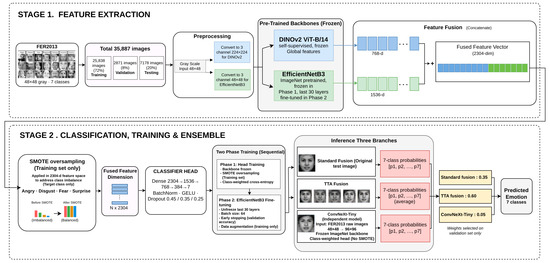
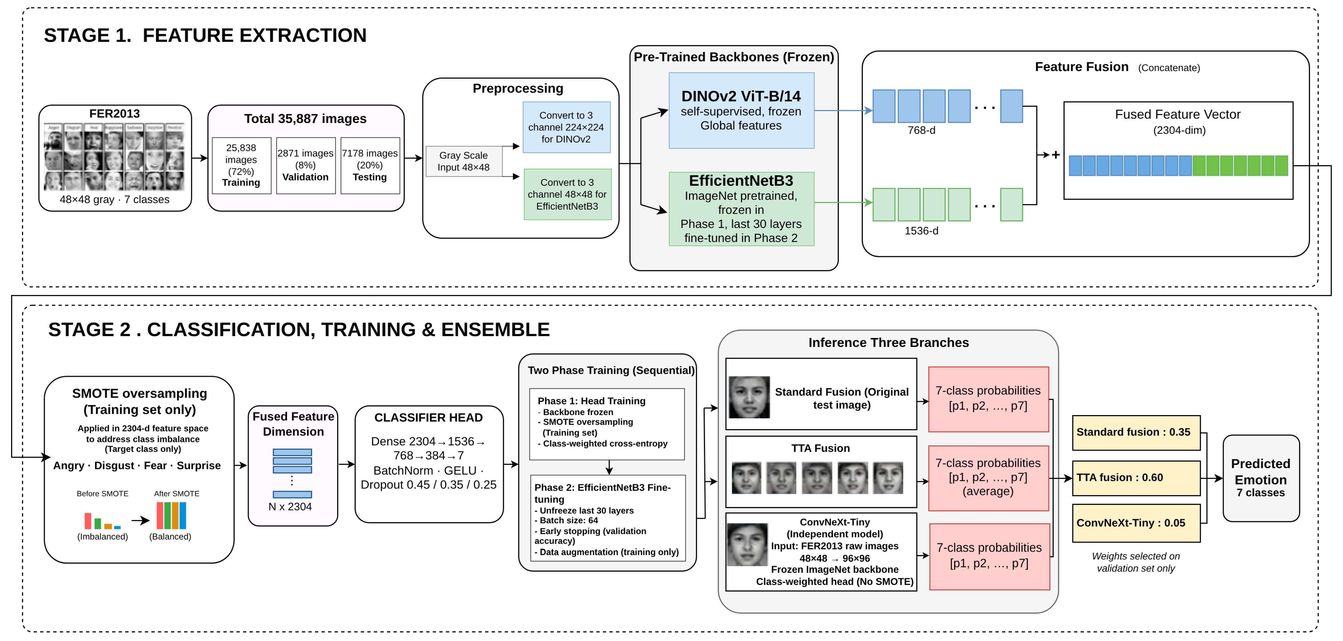
Figure 1 illustrates the overall methodology, from data preprocessing and feature extraction to model training and ensemble prediction.
Figure 1.
Overall two-stage methodology pipeline for FER2013 facial-expression recognition, covering data preprocessing, dual-backbone feature extraction and fusion, model training, and ensemble prediction. Blue boxes denote the DINOv2 branch, and green boxes denote the EfficientNetB3 branch.
3.1. Dataset and Preprocessing
The framework was evaluated on the FER2013 benchmark. We used the image-folder release of FER2013 on Kaggle (https://www.kaggle.com/datasets/msambare/fer2013, accessed on 1 January 2026). This release is derived from the original ICML 2013 challenge data [27]. All images in this release were retained. No duplicate, corrupted, or ambiguous samples were removed, and no labels were changed. The dataset contains 48 × 48 grayscale images in seven emotion categories: angry, disgust, fear, happy, neutral, sad, and surprise. The provided training and test partitions were preserved, with 28,709 training images and 7178 test images. The executed image-folder release used in this study does not expose a separate PublicTest/PrivateTest distinction within the 7178-image test folder, so these images are referred to throughout the manuscript as the held-out test partition. Table 1 reports the class distribution of these partitions. The validation subset was subsequently created from the training partition, as described in Section 3.2. The data are imbalanced: disgust represents less than two percent of the training set, whereas happy represents more than one quarter, producing a near 16:1 ratio between the largest and smallest classes.
Table 1.
FER2013 class distribution by partition.
Each image was stored as an 8-bit grayscale array and replicated across three channels to match the input format of both pretrained backbones. This preserved the original luminance and texture information without introducing artificial color. The EfficientNetB3 branch was further adapted through Phase 2 fine-tuning. No additional face detection or cropping was applied because the FER2013 images were already cropped and approximately aligned to the face region. Two preprocessing pipelines were used to satisfy the input requirements of the feature-extraction backbones.
3.2. Data-Partitioning Protocol
To prevent test-set leakage during model selection, we reserved 10% of the training partition (2871 samples) as a held-out validation set using stratified sampling with a fixed random seed, leaving 25,838 images for model fitting. Of the 35,887 FER2013 images, 25,838 (72%) were, therefore, used for training, 2871 (8%) for validation, and 7178 (20%) for testing. The test partition was excluded from all model-selection decisions, including ensemble weights, early-stopping checkpoints, TTA configurations, and other training choices. The validation set was used for five decisions: early stopping in Phase 1, early stopping and learning-rate reduction in Phase 2, early stopping of the ConvNeXt-Tiny head, and the two ensemble-weight searches. The SMOTE threshold, the head architecture, and the five TTA views were set by design and were not selected through a search on the validation set. Because several decisions used the same validation set, some optimistic bias toward this split is possible. A separate tuning set or nested validation was not used because of the computational cost of the dual-backbone pipeline. All results come from one stratified split, and this is stated as a limitation in Section 5.
3.3. Dual Backbone Feature Extraction
Two pretrained backbones were used to extract complementary features from each image. The DINOv2 branch captures global semantic structure, and the EfficientNetB3 branch captures local texture. Their outputs are combined in Section 3.4.
3.3.1. DINOv2 Branch: Global Semantic Features
DINOv2 ViT-Base was used as the first feature extractor [28]. The vision transformer was pretrained with self-supervised distillation on a large uncurated image corpus and was kept frozen throughout training as a fixed feature extractor. Each grayscale image was converted to three channels, resized to 224 × 224 pixels, and normalized with standard ImageNet statistics before half-precision GPU inference. DINOv2 produced a 768-dimensional embedding representing global semantic structure.
3.3.2. EfficientNetB3 Branch: Local Texture Features
We used EfficientNetB3 as the second feature extractor [29]. It is a convolutional network pretrained on ImageNet and was selected over the smaller EfficientNetB0 variant used in an earlier baseline because its 1536-dimensional output captured richer local texture and edge information complementary to DINOv2. During initial feature extraction, EfficientNetB3 was frozen; images were kept at the FER2013 resolution of 48 × 48 × 3 pixels and passed through the Keras EfficientNet preprocessing function. This function leaves pixel values in the 0–255 range because EfficientNetB3 performs its own rescaling and normalization inside the network. The 48 × 48 input yields a 2 × 2 spatial map before global average pooling. It was kept because upsampling the small images did not add new facial detail.
3.4. Feature Fusion and Classification Head
As shown in Table 2, the classification head progressively reduces the 2304-dimensional fused representation through layers of 1536, 768, and 384 units before the seven-class output. This design provides sufficient capacity while gradually reducing the feature dimensionality. Because the head is relatively large compared with the training set, dropout, L2 regularization, label smoothing, and early stopping were applied to control overfitting. Overfitting was monitored using training and validation performance, and the checkpoint with the highest validation accuracy was retained. Smaller head architectures were not systematically evaluated and are acknowledged as a direction for future work. In the reported Phase 1 run, training accuracy reached 99.5% compared with 69.5% validation accuracy, indicating a substantial generalization gap.
Table 2.
Classification head architecture, backbone inputs and outputs, and parameter counts. Values in parentheses are trainable parameters.
3.5. Two-Phase Training Protocol
The fusion model was trained in two sequential phases. Phase 1 trained only the classification head on precomputed features, and Phase 2 fine-tuned the last layers of the EfficientNetB3 branch on raw images.
3.5.1. Phase 1: Head Training with Targeted Oversampling
In Phase 1, both backbones were kept frozen and only the classification head was trained on the precomputed fused features. Classes with fewer than 60% of the majority-class count were oversampled with SMOTE to that threshold [30]. The majority class (happy) contained 6493 training samples, giving a threshold of 3896; angry, disgust, fear, and surprise were, therefore, oversampled, while happy, neutral, and sad were unchanged. The 60% threshold was a heuristic and was not optimized. SMOTE was restricted within each minority class and applied only to the 2304-dimensional fused training features. Feature-space oversampling avoided generating synthetic low-resolution face images, and the synthetic feature vectors had no corresponding raw images; therefore, they were used only in Phase 1 and excluded from Phase 2. The effective training set increased from 25,838 to 30,893 samples, and class weights were recomputed after oversampling.
The head was optimized with Adam using cosine-decay learning, with an initial rate of 1 × 10⁻³ decayed over 60 epochs to 1 × 10⁻⁶, a batch size of 128, and early stopping based on validation accuracy with a patience of 20 epochs. The weights from the epoch with the highest validation accuracy were restored as the Phase 1 checkpoint.
3.5.2. Phase 2: Fine-Tuning of the EfficientNetB3 Branch
In Phase 2, DINOv2 remained frozen while the last 30 EfficientNetB3 layers (3,551,386 parameters) were unfrozen and fine-tuned end to end on raw pixel data. These layers form the final stage of the network, comprising the block 7 MBConv layers and the top 1 × 1 convolution with its batch normalization and activation. This setting adapted the final task-specific stage while keeping earlier layers frozen to limit overfitting on the small training set; the layer count was not tuned. The phase was warm-started from the Phase 1 head weights. On-the-fly augmentation comprised random horizontal flipping, random rotation up to ±14.4°, random zoom up to ±10%, and random translation up to ±8% of the image height and width. Adam was used with a learning rate of 5 × 10⁻⁶, batch size 64, the same class-weighted label-smoothed cross-entropy loss, early stopping with patience 8, and learning-rate reduction on plateau. The checkpoint with the highest validation accuracy was saved and restored. Validation accuracy was used as the stopping criterion in both phases; the use of accuracy rather than macro F1 is noted as a limitation in Section 5.
After fine-tuning, fused features for the training, validation, and test partitions were rebuilt using the updated EfficientNetB3 weights, and the fine-tuned head weights were transferred to the fused-input production model used for downstream evaluation. The training and validation curves for both phases are provided in Figure A1 (Appendix A).
3.6. Test-Time Augmentation
A five-view test-time augmentation (TTA) scheme was applied at inference [31]. Each image was evaluated in five variants: the original image, horizontal flip, +10% brightness, −10% brightness, and a 90% center crop. The brightness transformation was applied to the 8-bit grayscale image with clipping to 0–255, and each view was then resized and normalized using the same backbone-specific preprocessing as the original image. Rotations and larger crops were not used because of the limited spatial resolution of FER2013. Both DINOv2 and EfficientNetB3 received the same augmented view to avoid branch mismatch. The five predicted-probability sets were averaged to obtain the final TTA prediction. Individual TTA views were not evaluated separately, and this is noted as a limitation in Section 5.
3.7. Ensemble Construction
The final ensemble combines the fusion model with a second, independently trained backbone. This section describes that backbone and the procedure used to select the ensemble weights on validation data.
3.7.1. Second Backbone: ConvNeXt-Tiny
The ConvNeXt-Tiny [32] branch was trained independently using the same training/validation protocol, with model selection and early stopping based exclusively on the held-out validation partition. It was included to add architectural diversity because its convolutional inductive bias differs from those of DINOv2 and EfficientNetB3, providing a complementary prediction pattern.
ConvNeXt-Tiny (27,820,128 parameters) was kept frozen. The branch was trained on raw images without SMOTE, and inputs were resized to 96 × 96 pixels. Globally average-pooled features were passed to a two-layer head with 512 and 256 units, batch normalization, GELU, and dropout of 0.4 and 0.3, respectively. The head was trained for up to 40 epochs with batch size 128, class weighting, Adam at 1 × 10⁻³, early stopping, and learning-rate reduction on plateau. The backbone used the Keras ConvNeXt-Tiny ImageNet-1k weights with global average pooling, producing a 768-dimensional feature vector. The 48 × 48 grayscale images were replicated to three channels and resized with bilinear interpolation. Pixel values were kept in the 0–255 range because the Keras ConvNeXt model includes its own normalization layer. The 96 × 96 size was chosen to reduce feature-extraction cost, since larger inputs would mainly upsample the same 48 × 48 content. The branch achieved 56.53% validation accuracy and 56.78% standalone test accuracy; this lower standalone performance is considered in the context of a frozen backbone and low-resolution upsampled inputs.
3.7.2. Validation-Based Ensemble-Weight Selection
Three ensemble configurations were evaluated in increasing complexity. First, a fixed, untuned 50/50 average of the fusion model and ConvNeXt-Tiny was computed as a fixed reference baseline because no test-informed weight selection was involved. It reached 75.13% test accuracy.
Second, a two-model ensemble was constructed by searching held-out validation data over a fine-grained weight grid. The search used 0.02 increments from 0.00 to 1.00, giving 51 candidate fusion weights. Validation accuracy was the primary selection criterion, with macro F1 used as the tie-breaker. The best weights, 0.46 for the fusion model and 0.54 for ConvNeXt-Tiny, were frozen and applied to the test set, yielding 75.34% accuracy, a 0.21 percentage-point gain over the fixed baseline.
Third, a three-way ensemble combining standard fusion, five-view TTA fusion, and ConvNeXt-Tiny was constructed with the same validation-only grid search. The search used a constrained 0.05 grid with non-negative weights summing to one, giving 231 candidate weight combinations. Validation accuracy was the primary selection criterion, with macro F1 used as the tie-breaker. The best weights were 0.35, 0.60, and 0.05, respectively, and were frozen before one test-set evaluation. The final ensemble reached 76.51% test accuracy, 1.38 percentage points above the fixed baseline. During development, one diagnostic sweep of the two-model blend weight (0.30 to 0.85 in steps of 0.05) was run on the test set, directly after the fixed 50/50 ensemble had been evaluated. Its best weight was the same 0.50 used by the fixed baseline, so it gave no additional information. The sweep was run before the validation-based searches were designed. Those searches covered the full 0 to 1 range on validation data and did not use its output. It is reported here for transparency, and its result is not used anywhere in this paper.
On the held-out validation set, the fixed 50/50 ensemble achieved 74.61% accuracy (macro F1 74.41%), while the validation-tuned two-way blend achieved 75.44% accuracy (macro F1 75.11%) with weights of 0.46 and 0.54 for fusion and ConvNeXt-Tiny, respectively. These values were recorded during the executed weight-search run. The weight-search output for the final three-way configuration was retained, including the selected weights. However, its logged validation metric could not be independently reconciled with the available validation records, including the recorded validation results of the individual components, and is, therefore, not reported as a verified validation result. The final three-way weights were frozen before the single test-set evaluation.
3.8. Evaluation Protocol and Metrics
We obtained all reported final results by applying the validation-selected model to the 7178-image FER2013 test partition. We did not use the test labels to select ensemble weights, early-stopping checkpoints, TTA configurations, or other model-selection decisions; we made these decisions exclusively using the training and held-out validation partitions. We summarized performance with accuracy, macro and weighted precision, recall, and F1, plus Cohen’s kappa. We assessed class discrimination with one-vs-rest ROC curves and macro ROC AUC. We assessed calibration with expected calibration error, multiclass Brier score, and a reliability diagram [33,34,35]. Accuracy and macro F1 uncertainty were quantified using 2000-resample bootstrap 95% confidence intervals [36,37], and paired-model differences were tested with McNemar’s test [38]. We also checked prediction accuracy against the confusion-matrix trace, and they agreed in terms of numerical precision.
3.9. Reproducibility
A global random seed of 42 was applied to Python’s random module (Python 3.13.15), NumPy 2.1.3, TensorFlow, and PyTorch before data loading or model construction and was reused for the stratified split, SMOTE, and model initialization. Exact bitwise GPU reproducibility was not guaranteed because some cuDNN kernels were non-deterministic. The fixed seed makes the reported run repeatable, but it does not show that the result is robust. Results across several seeds or repeated validation splits were not computed because each full run of the pipeline requires many GPU hours. This is listed as a limitation in Section 5. All experiments were run on a NVIDIA Tesla T4 GPU (NVIDIA Corporation, Santa Clara, CA, USA) with TensorFlow 2.20.0, Keras 3.13.2, and PyTorch 2.10.0 built against CUDA 12.8. The complete code, including the preprocessing scripts, package versions, split indices, random seeds, and trained checkpoints, will be released in a public GitHub repository upon publication of this article.
4. Results
This section reports the performance of the final ensemble on the FER2013 test partition. It then examines the contribution of each component, the class-level errors, discrimination, calibration, the SMOTE ablation, and the comparison with prior work.
4.1. Overall Performance
The final model was a validation-tuned three-way ensemble of standard DINOv2–EfficientNetB3 fusion, five-view TTA fusion, and ConvNeXt-Tiny. It was evaluated on the 7178-image FER2013 test partition. The test labels were not used for model selection. Table 3 reports the metrics. The ensemble reached 76.51% accuracy (95% CI 75.49–77.49), macro F1 75.77% (95% CI 74.48–76.99), weighted F1 76.32%, Cohen’s kappa 0.7158, and macro ROC AUC 0.9574.
Table 3.
Final test metrics, validation-tuned three-way ensemble (n = 7178).
4.2. Contribution of Individual Components
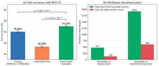
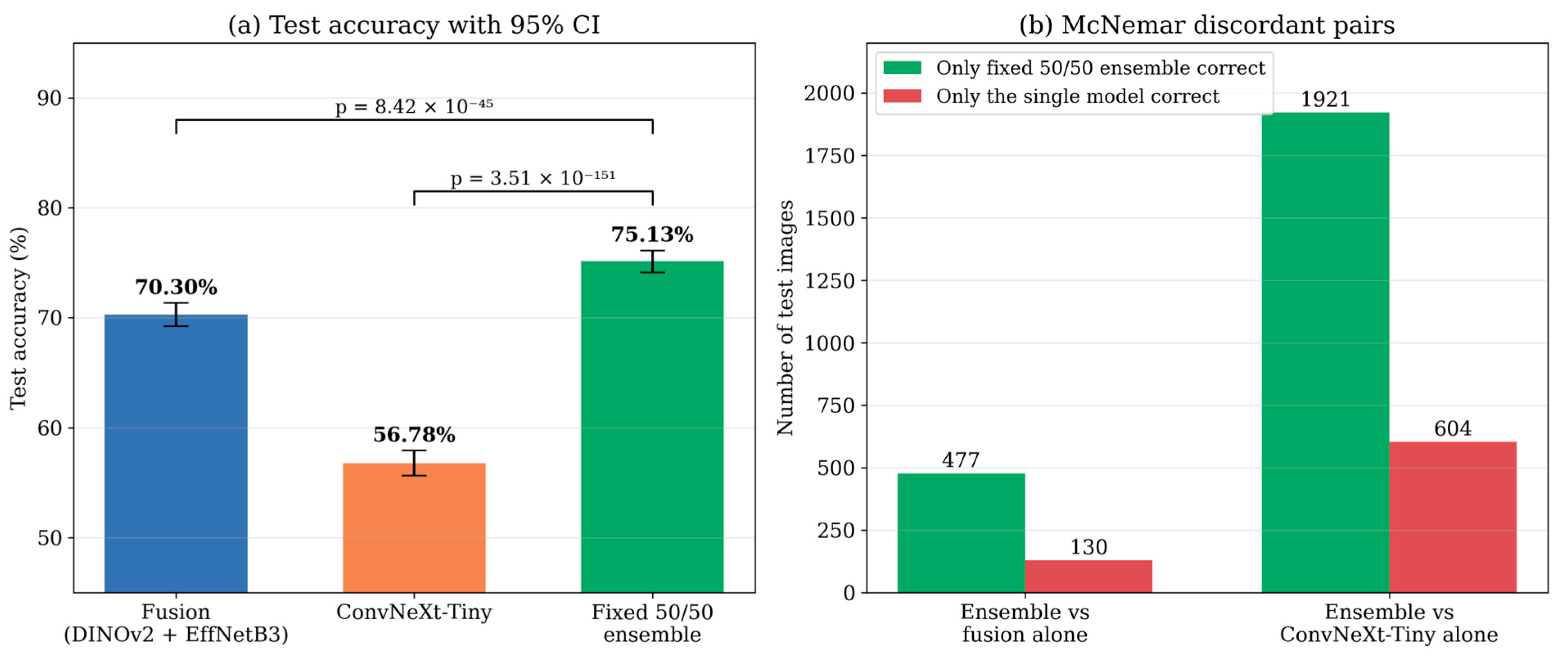
Figure 2 visualizes model accuracy with 95% confidence intervals and the McNemar discordant-pair counts. The fixed ensemble corrected 477 images missed by fusion alone while losing 130 images fusion classified correctly; it corrected 1921 images missed by ConvNeXt-Tiny while losing 604. Both differences are tested in Section 4.6. These gains were measured on one data split with one random seed. They should, therefore, be read as a promising result rather than as a confirmed robust improvement.
Figure 2.
Accuracy of the fusion model, ConvNeXt-Tiny, and its fixed 50/50 ensemble, with 95% confidence intervals (a), and the corresponding McNemar discordant-pair counts (b). The Figure refers to the fixed 50/50 fusion–ConvNeXt-Tiny ensemble and not to the final three-way ensemble. The intervals are Wilson-score intervals, and the p-values are from McNemar’s test before Holm correction.
The weight pattern reflects both standalone strength and complementary prediction behavior. As shown in Table 4, fusion reaches 70.30% versus 56.78% for ConvNeXt-Tiny, yet validation assigned ConvNeXt-Tiny a weight of 0.54 in the two-model ensemble. After TTA fusion was added, validation shifted weight toward TTA fusion (0.60), retained 0.35 for standard fusion, and reduced ConvNeXt-Tiny to 0.05. The nonzero ConvNeXt-Tiny weight indicates that its predictions contributed to the validation-selected combination. The most direct evidence of complementarity in this study is the paired-correction analysis in Figure 2, where the fixed ensemble corrected 477 test images missed by fusion alone while losing 130. A direct measure of pairwise disagreement or error overlap between the fusion model and ConvNeXt-Tiny was not computed and is left for future work.
Table 4.
Standalone and ensemble configurations with validation and test accuracy.
4.3. Confusion Matrix Analysis
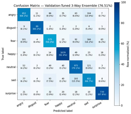
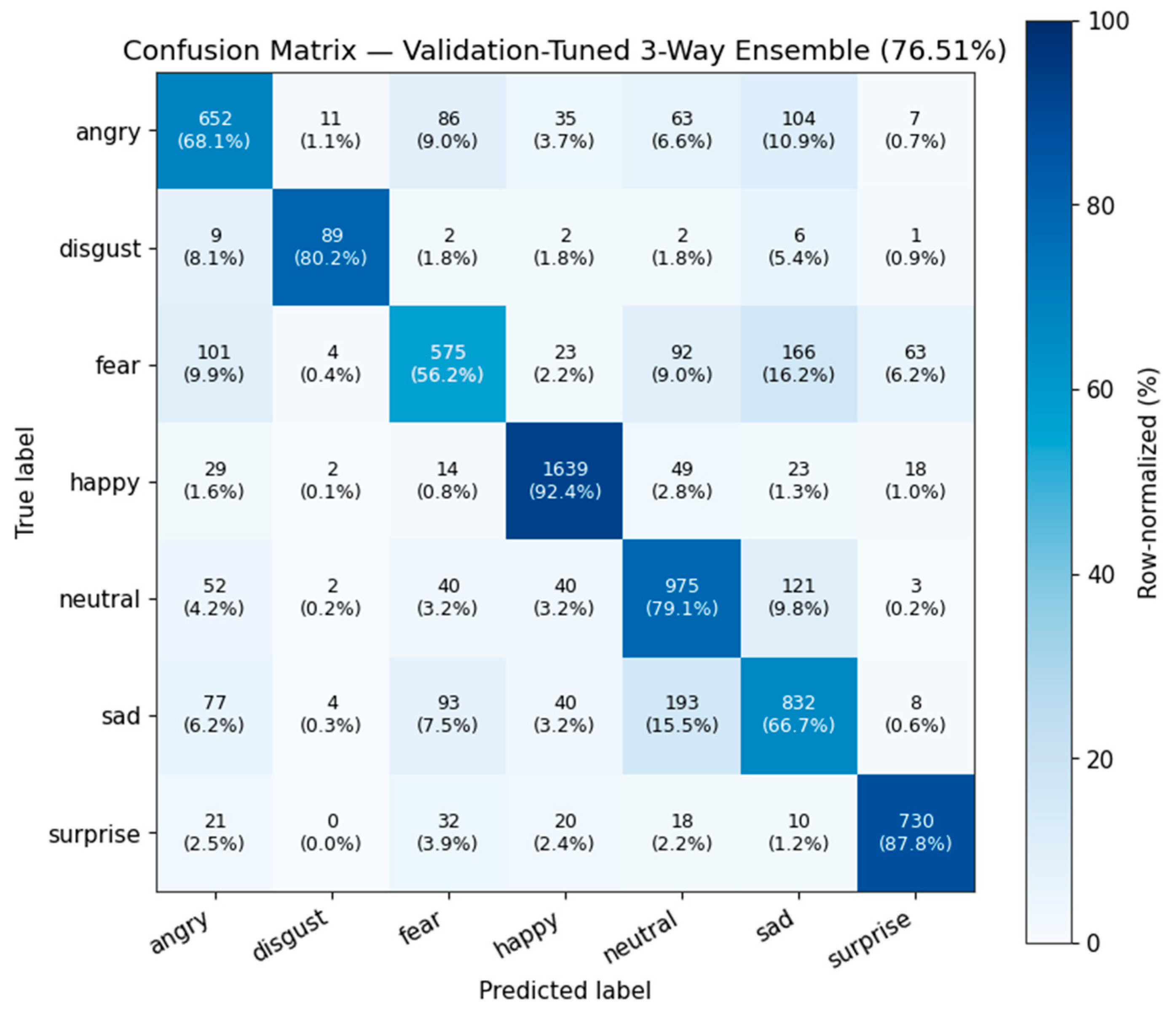
The class-wise error analysis reveals clear differences in recognition performance across emotions. The row-normalized confusion matrix in Figure 3 shows that recall is highest for happy (92.4%) and surprise (87.8%) and lowest for fear (56.2%). Fear is most often confused with sad (16.2%) and angry (9.9%), while 15.5% of sad samples are predicted as neutral. Disgust achieves 80.2% recall despite representing less than two percent of the training data. One possible explanation is the targeted Phase 1 oversampling. However, matched class-level results with and without SMOTE are not available (Section 4.10), so this link is not confirmed.
Figure 3.
Row-normalized confusion matrix for the final validation-tuned three-way ensemble on the test set. The corresponding raw-count matrix is given in Figure A2 (Appendix A).
4.4. Per-Class Performance
Table 5 reports per-class precision, recall, F1, and 95% bootstrap confidence intervals. The intervals are narrowest for the majority classes, happy and neutral, and widest for disgust, which has 111 test images.
Table 5.
Per-class classification report with 95% bootstrap confidence intervals. Precision intervals are Wilson-score intervals computed from the confusion-matrix counts. The last column gives the one-vs-rest ROC AUC of each class.
4.5. Discriminative Ability: ROC Analysis
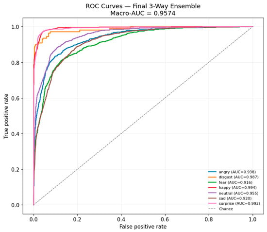
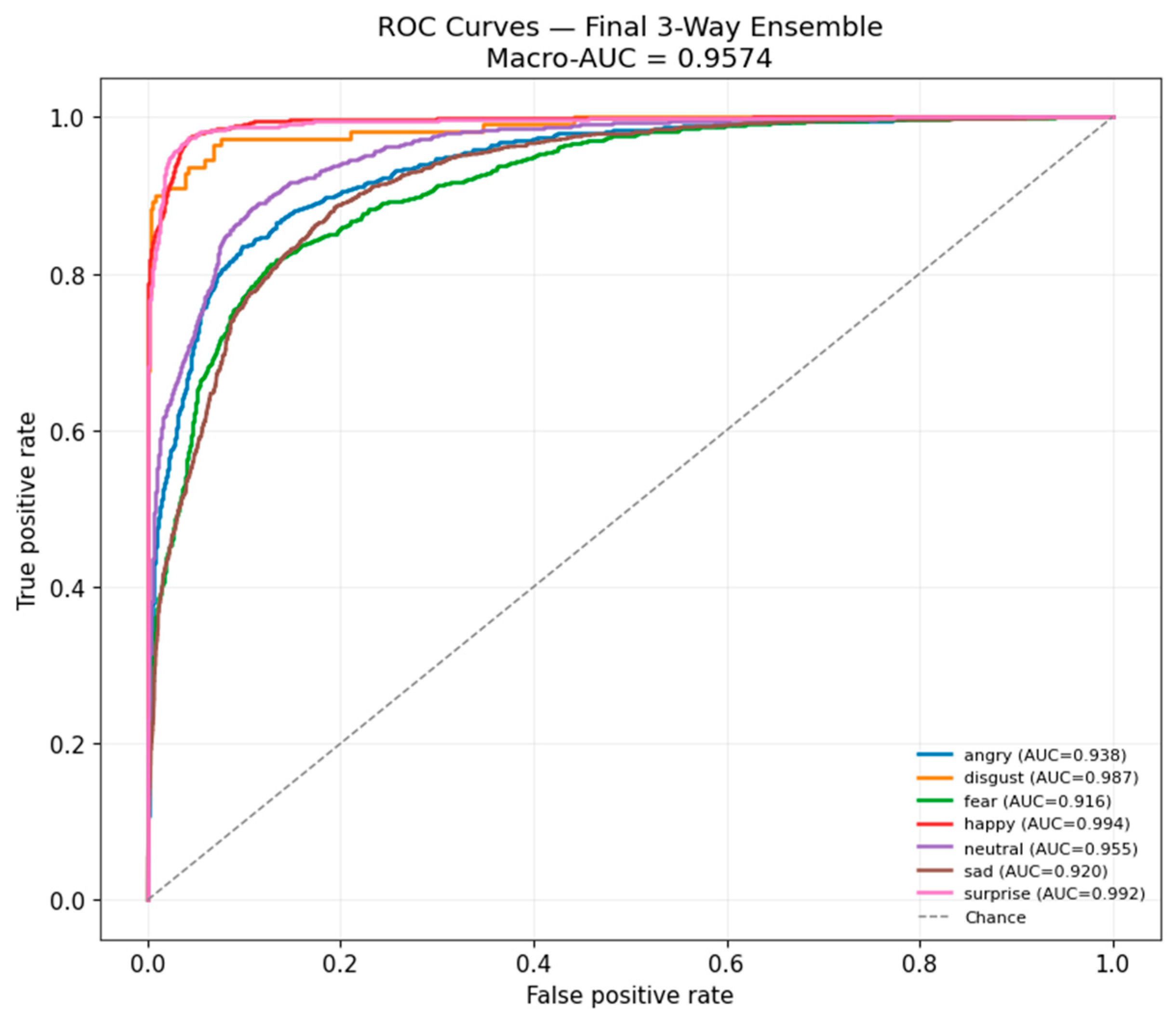
Figure 4 presents one-vs-rest ROC curves for all seven classes. Each class exceeds an AUC of 0.90; happy (0.994), surprise (0.992), and disgust (0.987) are the most separable, whereas fear (0.916) and sad (0.920) are the least separable, consistent with the confusion patterns in Section 4.3. The AUC of every class is also listed in Table 5, where angry reaches 0.938 and neutral 0.955. Precision-recall curves were not included in this revision. Instead, Table 5 reports per-class precision and recall with 95% confidence intervals, which reflect the same trade-off under class imbalance.
Figure 4.
One-vs-rest ROC curves per class for the final three-way ensemble.
4.6. Statistical Significance of the Final Ensemble
To further assess the paired-prediction difference between the final three-way ensemble and the fixed 50/50 baseline, we used McNemar’s test. Table 6 reports the paired counts and test statistic. The three-way ensemble is correct on 902 images missed by the baseline, whereas the baseline is correct on 803 images missed by the ensemble; the difference is statistically significant. McNemar’s test compares two fixed models on the same test images and does not measure variation across random seeds or data splits.
Table 6.
McNemar test, validation-tuned 3-way ensemble vs. fixed 50/50 baseline.
The two comparisons in Figure 2 were tested in the same manner. The fixed 50/50 ensemble’s advantage over fusion alone (477 corrected versus 130 lost) was statistically significant (McNemar p = 8.42 × 10−45), as was its advantage over ConvNeXt-Tiny alone (1921 corrected versus 604 lost; p = 3.51 × 10−151). Both comparisons show statistically significant paired-prediction differences between the models. Table 6 and these two comparisons form a family of three McNemar tests. After Holm correction for multiple comparisons, all three remain significant at the 0.05 level, with adjusted p-values of 0.018, 1.68 × 10−44, and 1.05 × 10−150, respectively. We also computed 95% confidence intervals for the paired-accuracy differences from the discordant counts. The final ensemble exceeds the fixed baseline by 1.38 points (95% CI 0.25 to 2.51). The fixed baseline exceeds fusion alone by 4.83 points (95% CI 4.17 to 5.50) and ConvNeXt-Tiny alone by 18.35 points (95% CI 17.04 to 19.65). The interval for the final gain is wide and lies close to zero, which supports the cautious reading in Section 4.2.
4.7. Model Calibration
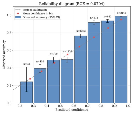
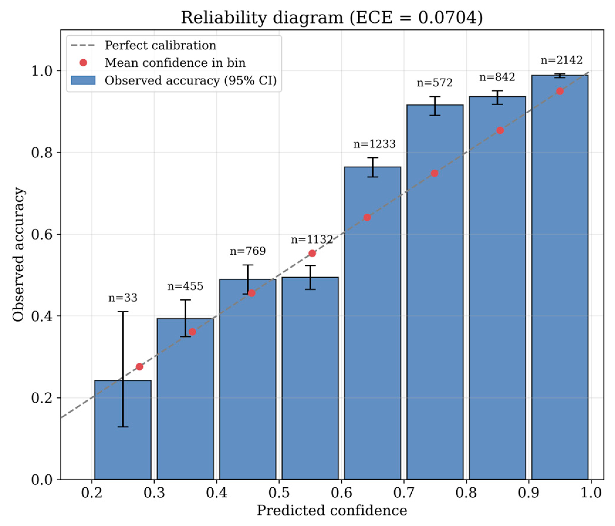
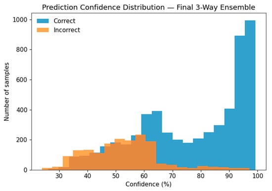
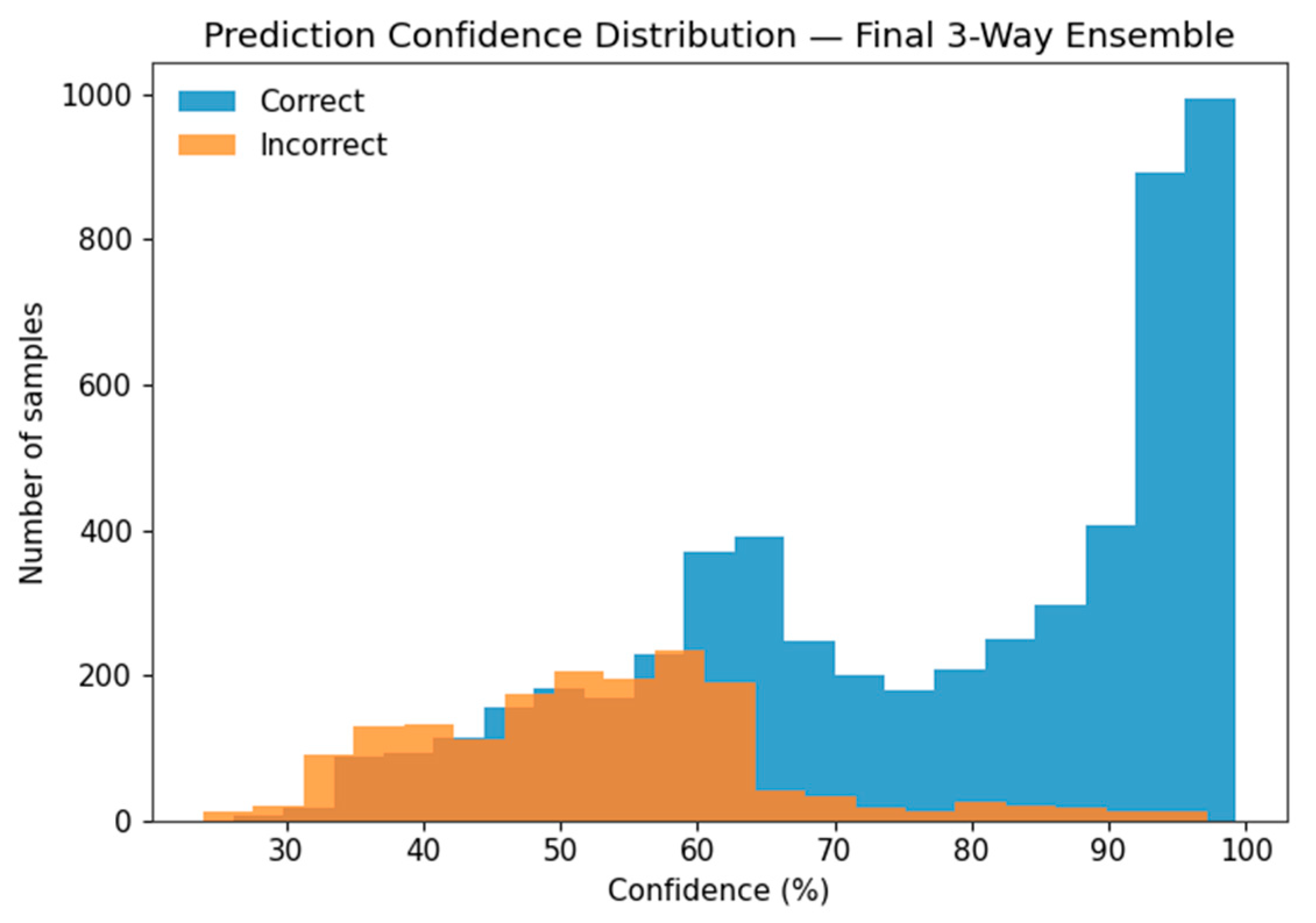
Calibration was assessed using expected calibration error, multiclass Brier score, and a reliability diagram. The final ensemble has an ECE of 0.0704 and a multiclass Brier score of 0.3209. Table 7 and Figure 5 show clear underconfidence in the 0.6–0.8 range, where empirical accuracy exceeds mean predicted confidence by 12–17 percentage points, and close calibration in the 0.9–1.0 bin, which contains the largest share of test predictions. The model is, therefore, not perfectly calibrated. The 0.6–0.8 range contains 1805 predictions, or 25.1% of the test set, and in this range the confidence scores understate the true accuracy by a large margin. Any use of these scores as decision thresholds would require recalibration, for example, by temperature scaling on validation data. Figure 6 shows that correct predictions have a higher mean confidence than incorrect predictions.
Table 7.
Calibration bins, final three-way ensemble.
Figure 5.
Reliability diagram for the final three-way ensemble (ECE = 0.0704). Bars show the observed accuracy in each confidence bin with 95% Wilson intervals, red points show the mean confidence, and n gives the number of test predictions in each bin.
Figure 6.
Prediction-confidence distribution for correct and incorrect predictions. Mean confidence is 77.06% for correct predictions versus 52.82% for incorrect predictions, a gap of 24.24 percentage points. The distributions contain 5492 correct and 1686 incorrect test predictions.
4.8. Error Analysis
The error analysis revealed several recurring patterns of confusion among visually similar expressions. As shown in Table 8, the two largest sources of error were sad→neutral and fear→sad, which together accounted for 359 of the 1686 test errors. Seven of the 15 confusion pairs involved sad, while six involved fear, highlighting these two classes as the primary targets for further improvement.
Table 8.
Top 15 confusion pairs, final three-way ensemble.
4.9. Qualitative Examples
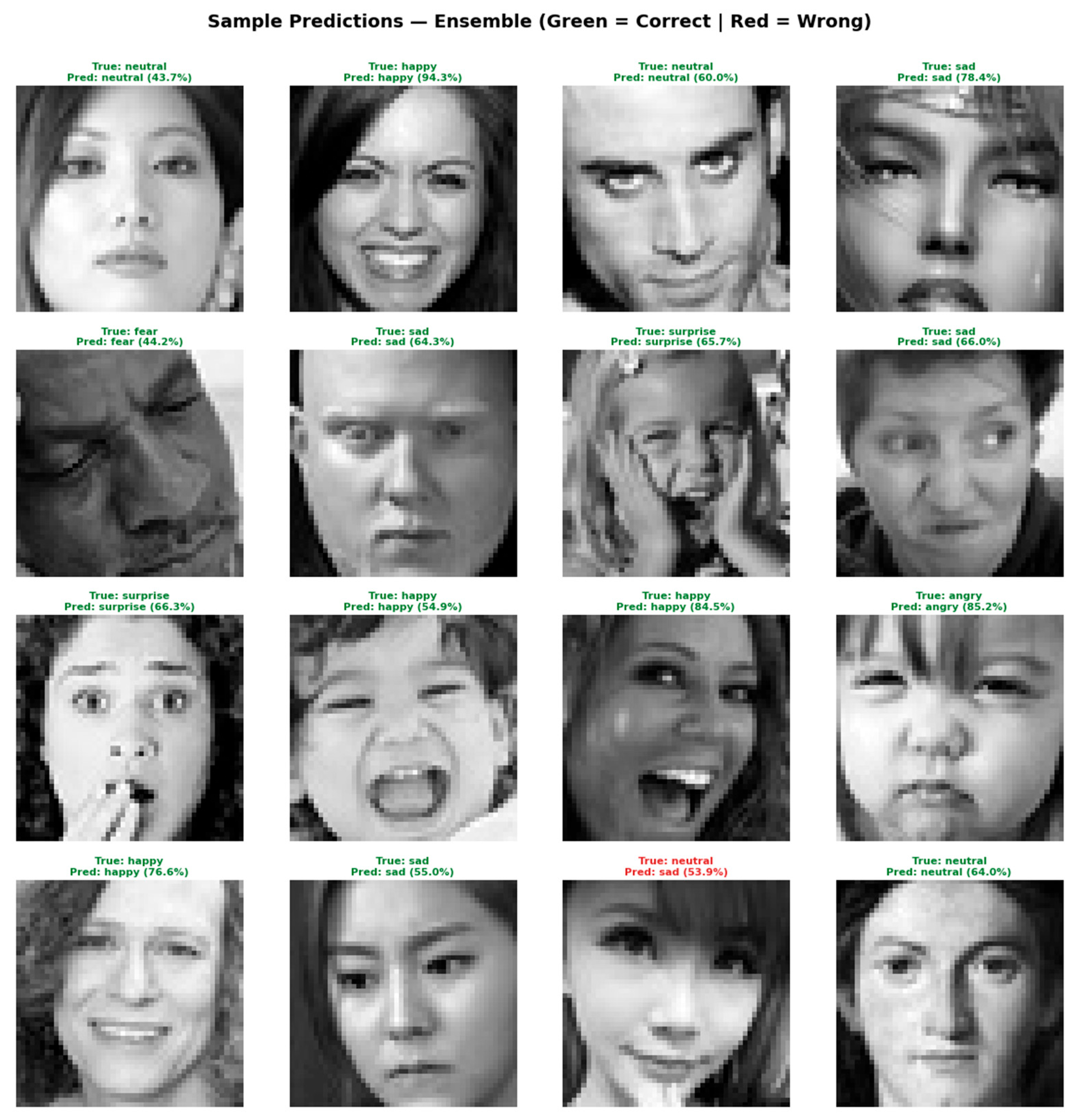
Figure 7 shows example test predictions from the fixed two-model ensemble stage, which is used here only for qualitative illustration, including true and predicted labels and confidence. Correct cases include a clearly posed happy expression at 94.3% confidence and lower-confidence cases near the decision boundary. The incorrect example is a neutral expression classified as sad at 53.9% confidence, illustrating the mid-confidence calibration weakness identified in Section 4.7.
Figure 7.
Example test predictions (green = correct, red = incorrect) with predicted class and confidence, from the fixed two-model ensemble (Section 3.7.2), not from the final three-way ensemble. The Figure only illustrates typical inputs and outputs. The 16 examples are not a representative sample of errors, such as those analyzed quantitatively in Section 4.3 and Section 4.8.
4.10. SMOTE Ablation
Section 3.5 describes targeted SMOTE in Phase 1, which raised angry, disgust, fear, and surprise to 60% of the majority-class count. To isolate its effect, a second head was trained on the same training and validation split with the Phase 1 architecture, optimizer, learning-rate schedule, and early-stopping policy, but without oversampling. Class imbalance was addressed only through the standard balanced class weighting.
The ablation head reached 70.18% validation accuracy, 0.66 percentage points above the 69.52% achieved by the SMOTE-trained Phase 1 head. Table 9 reports both configurations. Thus, targeted SMOTE did not improve aggregate validation accuracy for the fused feature representation and instead produced a small decrease.
Table 9.
Phase 1 validation metrics with and without SMOTE.
Table 10 gives the ablation head’s per-class metrics. A matching per-class breakdown was not recorded for the original SMOTE run, so only the aggregate accuracy values in Table 9 are directly comparable. The ablation head was trained in a separate session from the archived final-pipeline notebook; its aggregate and per-class results were taken from that session’s saved output rather than independently re-derived from the archived notebook.
Table 10.
Per-class validation metrics, Phase 1 head without SMOTE.
Despite the ablation result, the final pipeline retains Phase 1 SMOTE because Phase 2 and all subsequent stages were warm-started from the SMOTE-trained weights. Removing SMOTE would, therefore, require retraining the pipeline from Phase 1. Whether removing SMOTE improves the final ensemble, rather than only the Phase 1 head, remains an open question for future work. Because matched per-class results for the SMOTE-trained head are not available, the present evidence does not show that SMOTE benefits the minority classes. Its retention reflects the warm-start dependency described above rather than a demonstrated advantage.
4.11. Comparison with Prior Work
Table 11 compares the final validation-tuned three-way ensemble with 22 previously published FER2013 results from the literature reviewed in Section 2, ordered by reported test accuracy.
Table 11.
Comparison with previously published FER2013 results. Data splits, preprocessing, and the use of the test partition are not reported consistently across these studies and could not be verified for every entry, so the values are not strictly comparable. Ours * uses the 28,709/7178 partition with a 10% stratified validation split taken from the training partition, and the test partition was not used for model selection.
The proposed ensemble reports 76.51% accuracy, which is higher than the accuracies reported by the other studies listed in Table 11, including Wang et al. [26] (75.02%) and Chen et al. [25] (74.95%). Several other methods reach 72–73% using EfficientNet or ConvNeXt backbones. The observed difference may reflect the combined effect of the validation-only ensemble protocol, architectural diversity, and other pipeline choices; the individual contributions cannot be separated from this comparison. Because the listed studies differ in terms of preprocessing, data splits, augmentation, and tuning procedures, and these details are not always fully reported, this difference should not be interpreted as evidence of superiority under a matched protocol.
4.12. Scope of the Confidence Analysis
The confidence analysis in Section 4.7 suggests one possible use of the ensemble scores; namely, selective prediction in which low-confidence cases are deferred to a human reviewer. This is a benchmark observation only. FER2013 contains static, low-resolution web images, and it does not represent driving, clinical, or monitoring conditions. The present results, therefore, do not show that the model is suitable for such applications. Any application would first require validation on in-domain data collected under the target conditions, together with recalibration and an assessment of demographic bias.
5. Discussion
The result is consistent with a possible benefit from combining different inductive biases under a validation-based weighting protocol that excludes test labels from weight selection, although the individual effects of the ensemble components cannot be isolated.
The ablation in Section 4.2 provides a useful comparison. The fixed 50/50 fusion–ConvNeXt-Tiny blend reached 75.13%, which is close to the final three-way ensemble, while adding TTA and retuning the weights added 1.38 points. This observed pattern is consistent with a possible contribution from architectural diversity, but its individual effect cannot be separated from the simultaneous changes in TTA, ensemble composition, and weights. Thus, limited-compute settings may capture much of the observed benefit with a simple fixed blend rather than an extensive weight search.
The calibration results (ECE 0.0704 and Brier score 0.3209) indicate that confidence tracks accuracy only approximately. Together with the error analysis showing that fear and sad account for much of the confusion, these results suggest that confidence scores could help identify uncertain predictions. As discussed in Section 4.12, this remains a benchmark observation and does not establish suitability for real-world decision support.
The evaluation is limited to FER2013 and its predefined test partition. Because the images are small, grayscale, and collected from uncontrolled web sources, we did not measure performance on higher-resolution video or populations not represented in training. The backbones were also not evaluated under downstream deployment constraints such as embedded inference latency and memory footprint. These limitations define future validation needs.
Face analysis models can show accuracy differences across demographic groups [39,40]. The FER2013 labels are also partly ambiguous, which limits the accuracy that any model can achieve on this benchmark [41]. Facial-expression recognition also raises ethical concerns because facial movements do not map reliably onto internal emotional states [42]. Demographic bias could not be assessed with the available labels [39,40]. Such systems should, therefore, not be used in monitoring or decision-support settings without fairness evaluation and human oversight.
The study has further limitations. All results come from one stratified validation split and one random seed, so variation across splits and seeds was not measured. The same validation set was used for early stopping, learning-rate reduction, and both ensemble-weight searches, which may bias the selected configuration toward this split. The logged validation metric of the final three-way weight search could not be independently reconciled with the available validation records. Therefore, the selected weights and final test performance are reported without an unverified validation statistic (Section 3.7.2). Checkpoints were selected based on validation accuracy rather than macro F1, which may favor the majority classes. The full pipeline was not rerun without SMOTE, smaller classification heads were not compared, and the five TTA views were not evaluated individually. FER2013 contains low-resolution web images with limited demographic information. Performance may, therefore, differ across age groups, genders, ethnicities, lighting conditions, and is dependent on image quality.
6. Conclusions
This study presented a validation-based FER2013 framework that combines global semantic features from a frozen DINOv2 vision transformer with local convolutional features from EfficientNetB3, followed by partial fine-tuning, five-view test-time augmentation (TTA), and an independently trained ConvNeXt-Tiny branch. The final three-way ensemble used weights selected exclusively on the held-out validation set and achieved 76.51% accuracy, 75.77% macro F1, 76.32% weighted F1, Cohen’s kappa of 0.7158, and macro ROC AUC of 0.9574 on the 7178-image FER2013 test partition. The results show a promising gain over the fixed 50/50 ensemble and the fusion model, while the paired-error analysis is consistent with complementary prediction behavior. However, the individual effects of architectural diversity, TTA, ensemble composition, and weight selection cannot be isolated from the present experiments, and the SMOTE ablation does not establish an independent positive contribution to the final pipeline. The findings are limited to FER2013, one stratified validation split, and one random seed. Future work should evaluate the framework across additional FER datasets, repeated splits and seeds, and realistic in-domain data before drawing conclusions about real-world affect-aware or decision-support applications.
Author Contributions
Conceptualization, H.M.S.; methodology, H.M.S.; software, H.M.S.; validation, H.M.S.; formal analysis, H.M.S. and H.A.A.; investigation, H.M.S. and H.A.A.; resources, H.A.A.; data curation, H.M.S.; writing—original draft preparation, H.M.S. and H.A.A.; writing—review and editing, H.M.S.; visualization, H.M.S.; and project administration, H.A.A. All authors have read and agreed to the published version of the manuscript.
Funding
This research received no external funding.
Institutional Review Board Statement
The study was reviewed by the Institutional Review Board of Superior University and determined to be exempt from further ethics review/approval. The study used the publicly available FER2013 dataset for secondary computational analysis, with no recruitment of participants or collection of new human data.
Informed Consent Statement
Not applicable. The study used a publicly available, de-identified dataset and did not involve recruitment or collection of new human-subject data.
Data Availability Statement
The FER2013 dataset used in this study is publicly available at https://www.kaggle.com/datasets/msambare/fer2013 (accessed on 1 January 2026). The dataset is not redistributed by the authors. The complete code, including the preprocessing scripts, package versions, split indices, random seeds, and trained checkpoints, will be released in a public GitHub repository upon publication of this article, subject to applicable repository and licensing requirements.
Conflicts of Interest
The authors declare no conflicts of interest.
Abbreviations
The following abbreviations are used in this manuscript:
| FER | facial-expression recognition |
| TTA | test-time augmentation |
| SMOTE | synthetic minority oversampling technique |
| ViT | vision transformer |
| ROC | receiver operating characteristic |
| AUC | area under the curve |
| ECE | expected calibration error |
| CNN | convolutional neural network |
| CI | confidence interval |
| GELU | Gaussian error linear unit |
| ICML | International Conference on Machine Learning |
| MBConv | mobile inverted bottleneck convolution |
| ML | machine learning |
Appendix A
Figure A1.
Training and validation accuracy (a) and loss (b) of the fusion model across both training phases. The dashed line marks the start of Phase 2 at epoch 61. Values are taken from the training log of the reported run.
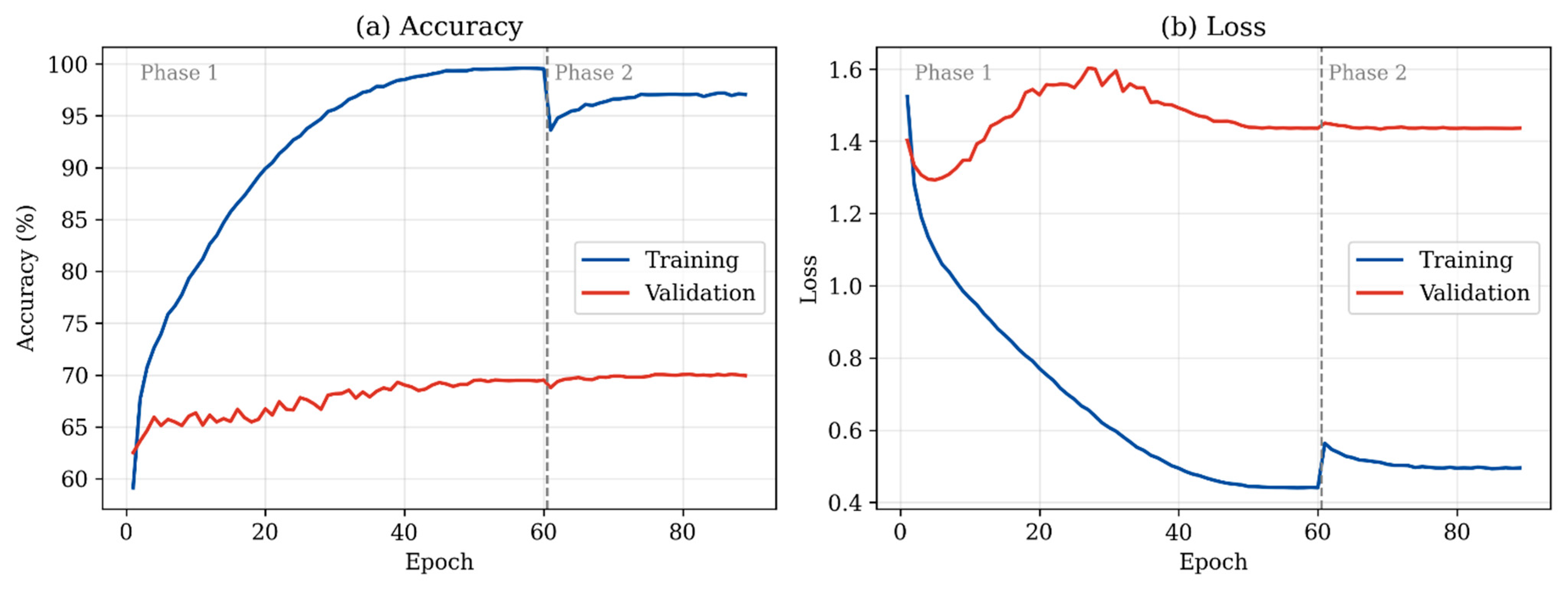
Figure A2.
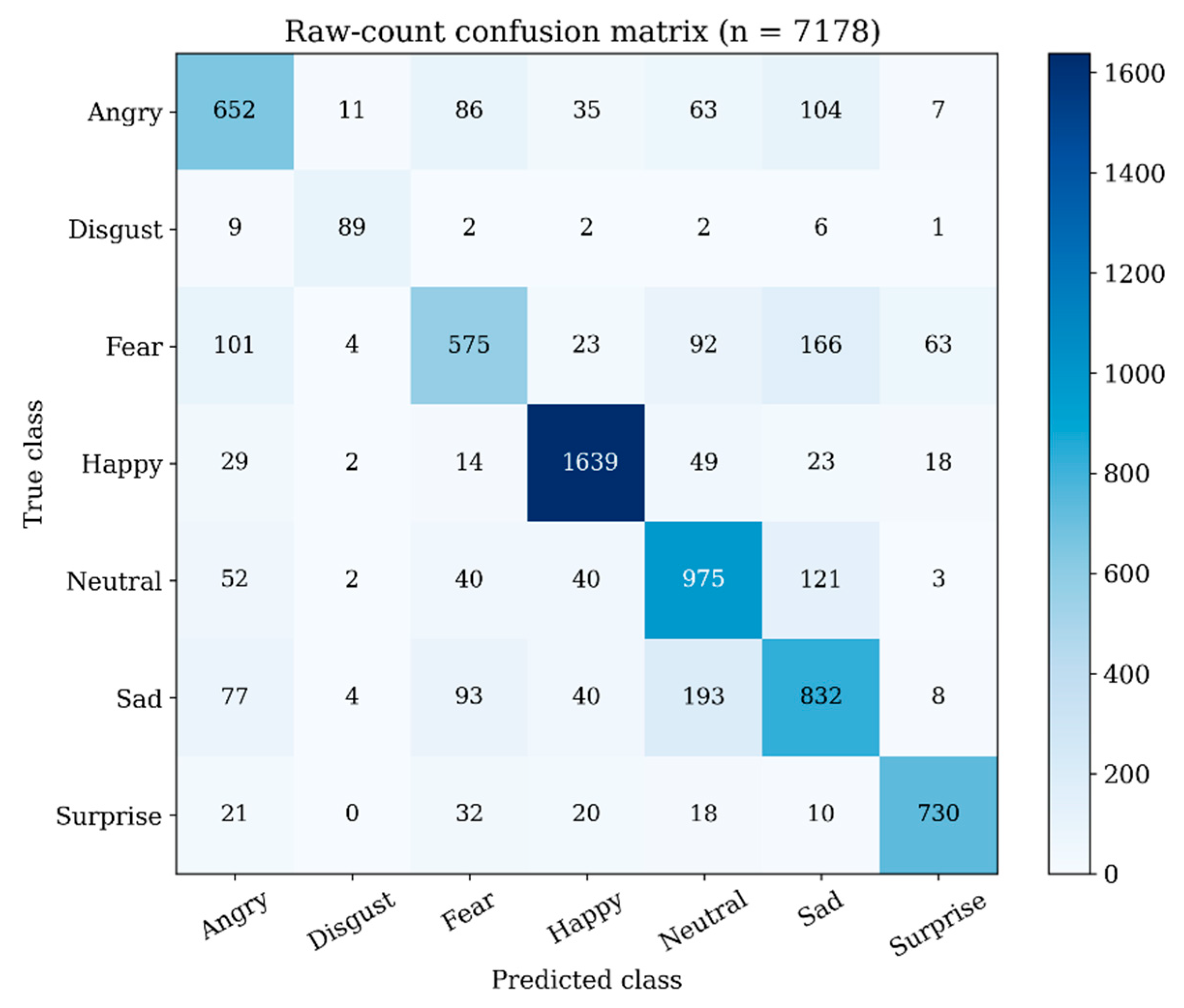
Raw-count confusion matrix of the final three-way ensemble on the FER2013 test set (n = 7178). Rows are true classes and columns are predicted classes. The diagonal contains 5492 correct predictions.
References
- Gursesli, M.C.; Lombardi, S.; Duradoni, M.; Bocchi, L.; Guazzini, A.; Lanatà, A. Facial Emotion Recognition (FER) Through Custom Lightweight CNN Model: Performance Evaluation in Public Datasets. IEEE Access 2024, 12, 45543–45559. [Google Scholar] [CrossRef] [Scilit]
- Banerjee, D.; Gothwal, P.; Biswas, A.K. ExpressNet-MoE: A hybrid deep neural network for emotion recognition. Mach. Learn. Appl. 2026, 23, 100830. [Google Scholar] [CrossRef] [Scilit]
- Agung, E.S.; Rifai, A.P.; Wijayanto, T. Image-based facial emotion recognition using convolutional neural network on emognition dataset. Sci. Rep. 2024, 14, 14429. [Google Scholar] [CrossRef] [Scilit]
- Qian, C.; Lobo Marques, J.A.; Fong, S.J. Analysis of deep learning algorithms for emotion classification based on facial expression recognition. In Proceedings of the 2024 8th International Conference on Big Data and Internet of Things (BDIOT), Macao, China, 14–16 September 2024; pp. 161–167. [Google Scholar] [CrossRef] [Scilit]
- Kaur, M.; Kumar, M. Facial Emotion Recognition Using the Lightweight EfficientNetB3 Model with FER-2013 and CK+ Datasets. Natl. Acad. Sci. Lett. 2026. [Google Scholar] [CrossRef] [Scilit]
- Chen, D.; Cao, Y.; Cheng, X. Research on Facial Expression Recognition Method Based on Improved ConvNeXt. IET Image Process. 2025, 19, e70118. [Google Scholar] [CrossRef] [Scilit]
- Jin, Y.; Qi, J. FER-YOLO: A YOLO-based classifier for facial expression recognition. Multimed. Syst. 2026, 32, 229. [Google Scholar] [CrossRef] [Scilit]
- Yen, C.-T.; Li, K.-H. Discussions of Different Deep Transfer Learning Models for Emotion Recognitions. IEEE Access 2022, 10, 102860–102875. [Google Scholar] [CrossRef] [Scilit]
- Mutaliyev, Y.; Kalpeyeva, Z. Development of Lightweight Residual Convolutional Neural Network for Efficient Facial Emotion Recognition. Int. J. Adv. Comput. Sci. Appl. 2026, 17, 776. [Google Scholar] [CrossRef] [Scilit]
- Ning, C.; Kok, V.J.; Chan, C.S. Enhancing Facial Expression Recognition Under Data Uncertainty Based on Embedding Proximity. IEEE Access 2024, 12, 85324–85337. [Google Scholar] [CrossRef] [Scilit]
- Mozaffari, L.; Brekke, M.M.; Gajaruban, B.; Purba, D.; Zhang, J. Facial Expression Recognition Using Deep Neural Network. In Proceedings of the 2023 3rd International Conference on Applied Artificial Intelligence (ICAPAI), Halden, Norway, 2 May 2023; pp. 1–9. [Google Scholar] [CrossRef] [Scilit]
- Salami, A.N.; Jabbar, A.; Mohamed, A. Enhanced Facial Expression Recognition Using Multi-Scale Attention Fusion and Deep Learning. Int. J. Comput. Inf. Syst. Ind. Manag. Appl. 2026, 18, 188–200. [Google Scholar]
- Ramdas, P.; Harakannanavar, S.S.; Chikkanna, S.K.; Puranikmath, V.I. Optimizing deep learning models for facial emotion recognition in embedded systems. Rev. Comput. Eng. Res. 2026, 13, 69–83. [Google Scholar] [CrossRef] [Scilit]
- Nemati, R.; Shirini, K.; Gharehveran, S.S. FER-HA: A hybrid attention model for facial emotion recognition. J. Supercomput. 2025, 81, 1485. [Google Scholar] [CrossRef] [Scilit]
- Feng, Z. Application of Facial Expression Recognition in Real-World Environments: From Traditional Convolutional Networks to Vision Transformers. Appl. Comput. Eng. 2026, 234, 46–54. [Google Scholar] [CrossRef] [Scilit]
- Li, S.; Wang, J.; Tian, L.; Wang, J.; Huang, Y. A fine-grained human facial key feature extraction and fusion method for emotion recognition. Sci. Rep. 2025, 15, 6153. [Google Scholar] [CrossRef] [Scilit]
- Zheng, C.; Mendieta, M.; Chen, C. POSTER: A Pyramid Cross-Fusion Transformer Network for Facial Expression Recognition. In Proceedings of the IEEE/CVF International Conference on Computer Vision Workshops (ICCVW), Paris, France, 2–6 October 2023; pp. 3138–3147. [Google Scholar] [CrossRef] [Scilit]
- Ding, J.; Zhang, T.; Yang, L.; Hu, T. A multiscale and multilevel fusion network based on ResNet and MobileFaceNet for facial expression recognition. IET Cyber-Phys. Syst. Theory Appl. 2025, 10, e70003. [Google Scholar] [CrossRef] [Scilit]
- Punuri, S.B.; Kuanar, S.K.; Kolhar, M.; Mishra, T.K.; Alameen, A.; Mohapatra, H.; Mishra, S.R. EfficientNet-XGBoost: An Implementation for Facial Emotion Recognition Using Transfer Learning. Mathematics 2023, 11, 776. [Google Scholar] [CrossRef] [Scilit]
- Tian, C.; Xie, J.; Li, L.; Zuo, W.; Zhang, Y.; Zhang, D. A Perception CNN for Facial Expression Recognition. IEEE Trans. Image Process. 2025, 34, 8101–8113. [Google Scholar] [CrossRef] [Scilit]
- Gharbi, A.; Gattal, A.; Bendib, I. Facial expression recognition for emotional state identification using deep convolutional neural network. Bull. Electr. Eng. Inform. 2026, 15, 384–395. [Google Scholar] [CrossRef] [Scilit]
- Tran, N.M.; Le, V.T. A Case Study of EmoNeXt-Tiny Without Self-Attention for Facial Emotion Recognition. Tech. Educ. Sci. 2026. [Google Scholar] [CrossRef] [Scilit]
- Gahlaut, A.; Rana, C.; Parihar, A.S.; Sharma, S. A Novel Approach for Facial Emotion Recognition: Deep CNN Feature Extraction Combined with ML Models. In Proceedings of the 2025 International Conference on Sustainable Communication Networks and Application (ICSCN), Theni, India, 15–17 October 2025; pp. 1463–1468. [Google Scholar] [CrossRef] [Scilit]
- Fan, A.; Kong, W.; Xiao, H.; Li, X. PHFNet: A Personality-Guided Hierarchical Fusion Network for facial expression recognition. Biomed. Signal Process. Control 2026, 123, 110369. [Google Scholar] [CrossRef] [Scilit]
- Chen, X.; Zheng, X.; Sun, K.; Liu, W.; Zhang, Y. Self-supervised vision transformer-based few-shot learning for facial expression recognition. Inf. Sci. 2023, 634, 206–226. [Google Scholar] [CrossRef] [Scilit]
- Wang, S.; Liu, M.; Ji, Z.; Wang, Y. Distilling Knowledge via Attention Transfer for Efficient Facial Expression Recognition in Classrooms. In Proceedings of the 2026 8th International Conference on Natural Language Processing (ICNLP), Xi’an, China, 20–22 March 2026; pp. 409–414. [Google Scholar] [CrossRef] [Scilit]
- Goodfellow, I.J.; Erhan, D.; Carrier, P.L.; Courville, A.; Mirza, M.; Hamner, B.; Cukierski, W.; Tang, Y.; Thaler, D.; Lee, D.-H.; et al. Challenges in Representation Learning: A Report on Three Machine Learning Contests. Neural Netw. 2015, 64, 59–63. [Google Scholar] [CrossRef] [Scilit]
- Oquab, M.; Darcet, T.; Moutakanni, T.; Vo, H.; Szafraniec, M.; Khalidov, V.; Fernandez, P.; Haziza, D.; Massa, F.; El-Nouby, A.; et al. DINOv2: Learning Robust Visual Features without Supervision. arXiv 2023, arXiv:2304.07193. [Google Scholar]
- Tan, M.; Le, Q.V. EfficientNet: Rethinking Model Scaling for Convolutional Neural Networks. In Proceedings of the 36th International Conference on Machine Learning (ICML), Long Beach, CA, USA, 9–15 June 2019; pp. 6105–6114. [Google Scholar]
- Chawla, N.V.; Bowyer, K.W.; Hall, L.O.; Kegelmeyer, W.P. SMOTE: Synthetic Minority Over-sampling Technique. J. Artif. Intell. Res. 2002, 16, 321–357. [Google Scholar] [CrossRef] [Scilit]
- Shanmugam, D.; Blalock, D.; Balakrishnan, G.; Guttag, J. Better Aggregation in Test-Time Augmentation. In Proceedings of the IEEE/CVF International Conference on Computer Vision (ICCV), Montreal, QC, Canada, 10–17 October 2021. [Google Scholar]
- Liu, Z.; Mao, H.; Wu, C.-Y.; Feichtenhofer, C.; Darrell, T.; Xie, S. A ConvNet for the 2020s. In Proceedings of the IEEE/CVF Conference on Computer Vision and Pattern Recognition (CVPR), New Orleans, LA, USA, 18–24 June 2022; pp. 11976–11986. [Google Scholar]
- Guo, C.; Pleiss, G.; Sun, Y.; Weinberger, K.Q. On Calibration of Modern Neural Networks. In Proceedings of the 34th International Conference on Machine Learning (ICML), Sydney, Australia, 6–11 August 2017; pp. 1321–1330. [Google Scholar]
- Brier, G.W. Verification of Forecasts Expressed in Terms of Probability. Mon. Weather Rev. 1950, 78, 1–3. [Google Scholar]
- Garcia-Gil, G. Minimal Angular Facial Representation for Real-Time Emotion Recognition. Appl. Sci. 2026, 16, 3572. [Google Scholar] [CrossRef] [Scilit]
- Efron, B.; Tibshirani, R.J. An Introduction to the Bootstrap; Chapman & Hall: New York, NY, USA, 1993. [Google Scholar]
- Arora, S.; Kieson, E.; Rudd, C.; Gloor, P.A. Multi-Modal Feature Fusion and Hierarchical Classification for Automated Equine–Human Interaction Behavior Recognition. Sensors 2026, 26, 2202. [Google Scholar] [CrossRef] [Scilit]
- McNemar, Q. Note on the Sampling Error of the Difference between Correlated Proportions or Percentages. Psychometrika 1947, 12, 153–157. [Google Scholar] [CrossRef] [Scilit]
- Buolamwini, J.; Gebru, T. Gender Shades: Intersectional Accuracy Disparities in Commercial Gender Classification. In Proceedings of the 1st Conference on Fairness, Accountability and Transparency, New York, NY, USA, 23–24 February 2018; pp. 77–91. [Google Scholar]
- Xu, T.; White, J.; Kalkan, S.; Gunes, H. Investigating Bias and Fairness in Facial Expression Recognition. In Computer Vision—ECCV 2020 Workshops; Springer: Cham, Switzerland, 2020; pp. 506–523. [Google Scholar] [CrossRef] [Scilit]
- Wang, K.; Peng, X.; Yang, J.; Lu, S.; Qiao, Y. Suppressing Uncertainties for Large-Scale Facial Expression Recognition. In Proceedings of the IEEE/CVF Conference on Computer Vision and Pattern Recognition (CVPR), Seattle, WA, USA, 13–19 June 2020; pp. 6897–6906. [Google Scholar] [CrossRef] [Scilit]
- Barrett, L.F.; Adolphs, R.; Marsella, S.; Martinez, A.M.; Pollak, S.D. Emotional Expressions Reconsidered: Challenges to Inferring Emotion from Human Facial Movements. Psychol. Sci. Public Interest 2019, 20, 1–68. [Google Scholar] [CrossRef] [Scilit]

Disclaimer/Publisher’s Note: The statements, opinions and data contained in all publications are solely those of the individual author(s) and contributor(s) and not of MDPI and/or the editor(s). MDPI and/or the editor(s) disclaim responsibility for any injury to people or property resulting from any ideas, methods, instructions or products referred to in the content. |
© 2026 by the authors. Licensee MDPI, Basel, Switzerland. This article is an open access article distributed under the terms and conditions of the Creative Commons Attribution (CC BY) license.