


Abstract
The Gulf of Mexico and the Caribbean Sea are key regions of the western Atlantic, where sea-state conditions are critical for coastal safety and offshore operations. This study analyzes wave climate trends (1981–2022) using WAVEWATCH III simulations validated against buoy observations. The Mann–Kendall test and Theil–Sen estimator were employed to quantify trends in significant wave height (Hs), energy period (Te), and wave power (P), while correlation analysis was performed to explore teleconnections with the Oceanic Niño Index (ONI), Atlantic Multidecadal Oscillation (AMO), and North Atlantic Oscillation (NAO). The results reveal basin-wide increases in mean Hs and P, characterized by pronounced spatial and seasonal heterogeneity. The most robust positive trends occur during winter and spring; in summer and fall, the weaker or negative tendencies, particularly in Te, suggest an intensification of seasonal contrasts rather than uniform change. Teleconnection analysis demonstrates that, among the climate indices considered in this study, ENSO is the primary driver of interannual wave variability in the Caribbean, particularly modulating wave power through remotely generated swell. While the NAO exerts regionally dependent control associated with storm-track modulation, the AMO plays a secondary role, affecting swell-dominated sectors. In contrast, the Gulf of Mexico shows limited sensitivity to large-scale climate modes, with wave variability largely governed by local wind–sea processes. These findings highlight the contrasting wave dynamics between these two basins, providing critical insights for coastal hazard assessments, maritime traffic along major shipping routes, oil spill management, and regional wave energy planning.
Keywords:
wave climate; Gulf of Mexico; Caribbean Sea; WAVEWATCH III; trend analysis; teleconnection 1. Introduction
The Gulf of Mexico (GoM) and the Caribbean Sea are key regions in the climate and oceanographic dynamics of the western Atlantic. Characterized by intense economic activity, these areas rely heavily on offshore oil extraction, commercial fishing, tourism, and critical marine transport routes, including high-density container shipping corridors. In the United States of America, coastal activities in the GoM contribute hundreds of billions of dollars to the gross domestic product (GDP). Similarly, Mexico derives substantial revenue from the region, with hydrocarbon and fishing exports alone exceeding several billion dollars annually [1]. Within this context, sea-state conditions are critical for maritime safety and logistics; extreme wave events, although relatively infrequent in the GoM compared to other basins, represent a non-negligible hazard to offshore infrastructure and navigation. Such events, including rogue waves, have been documented to cause severe damage to vessels and oil platforms, as well as loss of life [2,3]. Furthermore, both regions are highly vulnerable to extreme weather, particularly cold fronts and tropical cyclones, which drive storm surges and exacerbate coastal erosion [4,5,6]. This vulnerability is increasingly intensified by climate change, which modulates sea surface warming, ocean acidification, and the frequency of high-impact meteorological events [7].
On a global scale, an upward trend in wave power has been recorded, primarily attributed to sea surface warming and the reorganization of atmospheric circulation. Reguero et al. [8] demonstrated a direct correlation between ocean warming and the global increase in wave energy. Previous studies have documented shifts in wave climate at both global and regional scales [9,10].
Wave generation and propagation are intrinsically coupled to large-scale atmospheric and oceanic variability. Climate indices such as the El Niño–Southern Oscillation (ENSO), the AMO, and the NAO represent dominant modes of variability that modulate wind stress patterns, the cyclogenesis of wave-generating areas, and the swell propagation toward coastal regions. Significant correlations between these teleconnections and wave climate variability in the North Atlantic and its marginal seas have been documented. According to these studies, the regional response is the result of the overlap of multiple factors, whose impacts vary according to the specific sub-region and the wave parameters analyzed [11,12].
Prior studies on wave climate in the GoM and the Caribbean Sea have provided important but partial insights into regional wave dynamics. Appendini et al. [13] produced a comprehensive 30-year wave hindcast (1979–2008) driven by high-resolution reanalysis winds, showing that mean wave conditions in the GoM are primarily modulated by winter cold fronts, while extreme wave conditions are influenced by both tropical cyclones and cold fronts; in the Caribbean, they identified the Caribbean Low-Level Jet (CLLJ) as a key driver of mean wave heights. These fluctuations in Hs are also linked to large-scale climatic drivers, including ENSO phases and tropical cyclones activity [14]. Panchang et al. [15] developed a multi-decadal hindcast of Hs in the GoM, identifying contrasting trends between the eastern and western basin, with a focus on extreme conditions relevant for offshore engineering. In the Caribbean Sea, Montoya et al. [16] analyzed tropical cyclones-induced wave heights, showing that changes in tropical cyclone activity have led to spatially variable trends in extreme wave conditions.
Collectively, these studies highlight that previous research in the region has typically focused on individual wave parameters, specific forcing mechanisms, or sub-regions. An integrated, multi-variable assessment that simultaneously characterizes Hs, Te, and P across both basins on annual and seasonal timescales, and that quantifies their relationships with major climate modes, remains limited.
The present study aims to detect and analyze annual and seasonal trends in wave parameters in the GoM and the Caribbean Sea. To achieve this, it analyzes 42 years of wave hindcast data, simulated via the WAVEWATCH III (WW3) model [17] and validated against National Data Buoy Center (NDBC) observations [18]. Statistical methods, including the Mann–Kendall test [19] and the Theil–Sen slope estimator [20], are employed to identify and quantify these trends [21]. Finally, the interplay between the identified trends and the global climate indices (ENSO, AMO, and NAO) is examined to elucidate the long-term wave dynamics in the region.
The remainder of this paper is organized as follows: Section 2 describes the model setup, validation, and the statistical methodologies for trend and index correlations. Section 3 presents the results of the annual and seasonal trend analysis alongside the climate index correlation. Finally, Section 4 summarizes the main conclusions.
2. Materials and Methods
2.1. Numerical Model
This study used simulated data from the WW3 version 6.07 model (National Oceanic and Atmospheric Administration (NOAA), National Centers for Environmental Prediction, College Park, MD, USA) [17]. WW3 is a third-generation spectral wave model that solves the wave action balance equation. A forty-two-year hindcast (January 1981 to December 2022) was performed using wind forcing from the European Centre for Medium-Range Weather Forecasts (ECMWF) Reanalysis v5 (ERA5) [22]. The study period spans 42 years (1981–2022), exceeding the 30-year minimum recommended for climatological analyses and ensuring sufficient temporal coverage to characterize interannual and multidecadal wave climate variability.
2.1.1. Model Setup
The implementation of the WW3 model for the GoM and the Caribbean Sea employed a structured grid with a resolution of 0.1175°. The model domain spans from 9.00° N to 30.97° N in latitude and from 100° W to 63.45° W in longitude, covering the Gulf of Mexico and the Caribbean Sea. The wave spectrum was discretized into 24 uniformly spaced directions and 29 logarithmically distributed frequencies ranging from 0.0662 Hz to 0.9551 Hz, with a frequency increment factor of 1.1. It should be noted that the model frequency range may not fully capture swell energy associated with very long period waves (>16.7 s), which could represent a limitation in regions influenced by remote Atlantic swell, particularly the eastern Caribbean Sea. The bathymetry and obstacle grids, obtained from [23], have a resolution of 15 arcseconds. The coastline and island data were obtained from the Global Self-consistent, Hierarchical, High-resolution Shoreline Database (GSHHS) [24]. Wind forcing was derived from ERA5 [22], with a temporal resolution of one hour and a spatial resolution of 0.28°. The wind fields (0.28°) were bilinearly interpolated to the WW3 grid (0.1175°) and linearly interpolated to each source-term integration time step (30 min) following the model’s default schemes. The ST4 source term parameterization from Ardhuin et al. [25] was adopted, which includes formulations for wind input, whitecapping dissipation, nonlinear wave–wave interactions, and swell dissipation. This scheme is widely used in both global and regional wave modeling systems and has demonstrated robust performance in hindcast applications. It should be noted that the model grid not accounted swell propagation from the Atlantic Ocean into the Caribbean Sea in this simulation.
All simulations were performed on a high-performance workstation (Dell Precision T7920, Dell Technologies, Round Rock, TX, USA) equipped with dual Intel® Xeon® Silver 4215R processors (Intel Corporation, Santa Clara, CA, USA) (3.2 GHz), 256 GB of DDR4 RAM (2666 MHz, ECC).
WW3 employs four user-defined time steps, which in this study were set to: the global time step (1800 s), which synchronizes all sub-integrations and governs wind/current interpolation; the spatial propagation time step (900 s), which controls advection; the intra-spectral propagation time step (1350 s), which governs refraction and frequency-shifting within the spectrum; and the source-term integration time step (15 s), which acts as a minimum threshold for the dynamic point-by-point sub-stepping of source terms, allowing finer resolution under rapidly evolving conditions. The model outputs were saved at hourly intervals.
2.1.2. Validation Methodology
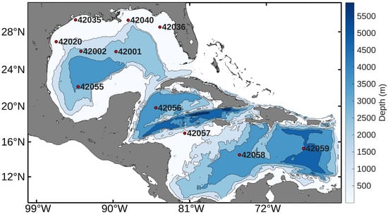
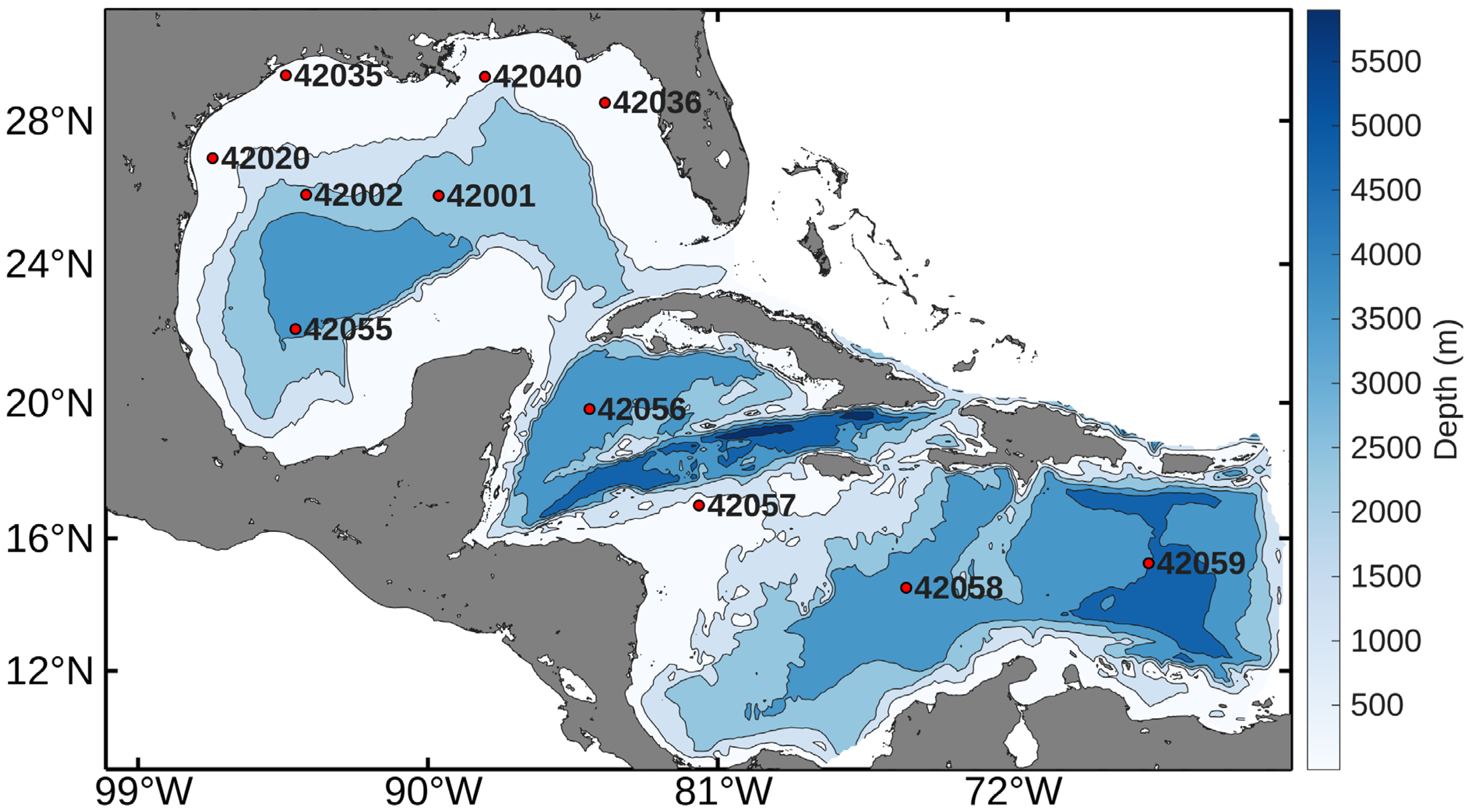
The WW3 model was validated by comparing the simulated data with hourly data from six NDBC buoys (Figure 1), focusing on the daily averages of Hs and the dominant wave period (Tp) between 1998 and 2022. The model’s performance was evaluated using the statistical metrics of mean bias, root mean square error (RMSE), and Pearson’s correlation coefficient (CC), defined as follows:
where N is the number of available observations, the upper bar indicates an average value, is the simulated variable, and is the observed variable. and are the standard deviation of the simulated and observed variables, respectively.
Figure 1.
Bathymetry of the study area and locations of NDBC buoys used for validation (red circles). Grey areas indicate land masses and inland water bodies outside the model domain.
2.2. Wave Energy Flux
The wave power density (P) was calculated for irregular waves, defined as:
where is the water density, is the gravitational acceleration, Hs is the significant wave height and Te is the energy period (, Te is approximated from Tp using the relationship , with [26].
2.3. Trend Analysis
The trends in Hs, Te, and P of the waves were estimated on an annual and seasonal basis. The Theil–Sen estimator was used to calculate the slopes of the trends, and the Mann–Kendall test was used to analyze statistical significance. Non-parametric methods were chosen because they are more suitable for independent datasets, unlike parametric methods, which require the data to follow a normal distribution. Since wave time series often exhibit serial correlation, a pre-whitening procedure was applied to reduce the influence of autocorrelation prior to the trend analysis, as described in Section 2.3.1.
2.3.1. Serial Correlation Effect
To mitigate the effects of serial correlation in time series data, this study adopts the pre-whitening approach proposed by von Storch and Navarra [27] prior to applying the Mann–Kendall test and Theil–Sen estimator. This approach reduces the influence of autocorrelation, leading to a more robust trend analysis.
In this procedure, the lag-1 serial correlation coefficient (denoted as ) is first estimated to quantify the degree of autocorrelation in the time series (), where represents the mean hourly wave model estimate at each grid point, following Kendall and Stuart [28] and Salas et al. [29]:
where is the mean of the sample data, and is the sample size.
If the calculated is significant, then the pre-whitened time series may be obtained as (
The critical value of depends on whether a one- or two-tailed test is applied. In a one-tailed test, the alternative hypothesis typically assumes that the true is greater than zero. In a two-tailed test, the alternative hypothesis posits that the true is not zero, without specifying whether it is positive or negative. The probability limits for in an independent series are calculated following the methods described by Salas et al. [29].
where n is the sample size.
The choice of alternative hypothesis depends on the specific characteristics of the problem. If previous tests suggest the presence of positive autocorrelation, it is preferable to use a one-tailed test. Otherwise, a two-tailed test is more appropriate, as it does not assume the direction of the autocorrelation.
2.3.2. Mann–Kendall Test
The Mann–Kendall S statistic was used to analyze the significance of the trend. This non-parametric test is widely used in hydrology and meteorology. is calculated as follows:
where is the number of data points; and are data values in the time series at times and , respectively; and the sign function is defined as
In cases where a time series contains repeated values, known as “tied groups,” the variance of is denoted as , and is computed as
where is the number of tied groups, and is the number of data points in the tied group. The Mann–Kendall statistic, , is usually assumed to be normally distributed for the datasets satisfying ; therefore, the transformation is employed as shown in Equation (11):
The value of can be positive, negative, or zero. Positive values indicate an increasing trend, negative values reflect a decreasing trend, and suggests no significant trend at the specified . In this study, a 95% confidence level was used for the statistical evaluations.
2.3.3. Theil–Sen Estimator
The Theil–Sen method estimates the median slope of data pairs in time series data. Both the slope and the intercept are calculated by computing a set of linear slopes, as described in Equation (5):
where is the number of data pairs in the time series, is the slope of the in the time series, and and are the data values at times and , respectively. For a dataset including one data point per pair , is calculated as shown in Equation (6):
where is the total number of data points in the time series. The Theil–Sen estimator is calculated as the median of the values of , as given in Equation (14):
The sign of indicates whether the data show an upward or downward trend, and the value shows the slope of that trend.
The magnitude of the trends was quantified using the Theil-Sen estimator. To provide a clearer representation of the changes over the 42-year study period, the results for Hs, Te and P are expressed in units per decade (e.g., m/10 years), consistent with common practices in long-term climate trend analysis.
2.4. Climate Indices
Monthly teleconnection indices, available from January 1950 to the present, were retrieved from the NOAA Physical Sciences Laboratory (https://www.psl.noaa.gov/, accessed on 5 February 2026). The ONI was employed to analyze ENSO variability [30]. Additionally the AMO index [31] and the NAO index [32] were incorporated. These datasets provide long-term metrics of climate variability widely recognized in atmospheric and oceanographic studies.
To evaluate the influence of large-scale climate variability, annual anomalies for wave parameters (Hs, Te, and P) were defined as the deviations from the long-term mean after removing the linear trend (detrended anomalies). These anomalies were then correlated with the respective climate indices (ONI, AMO, and NAO) at each grid point across the study domain.
3. Results and Discussion
3.1. Validation Results
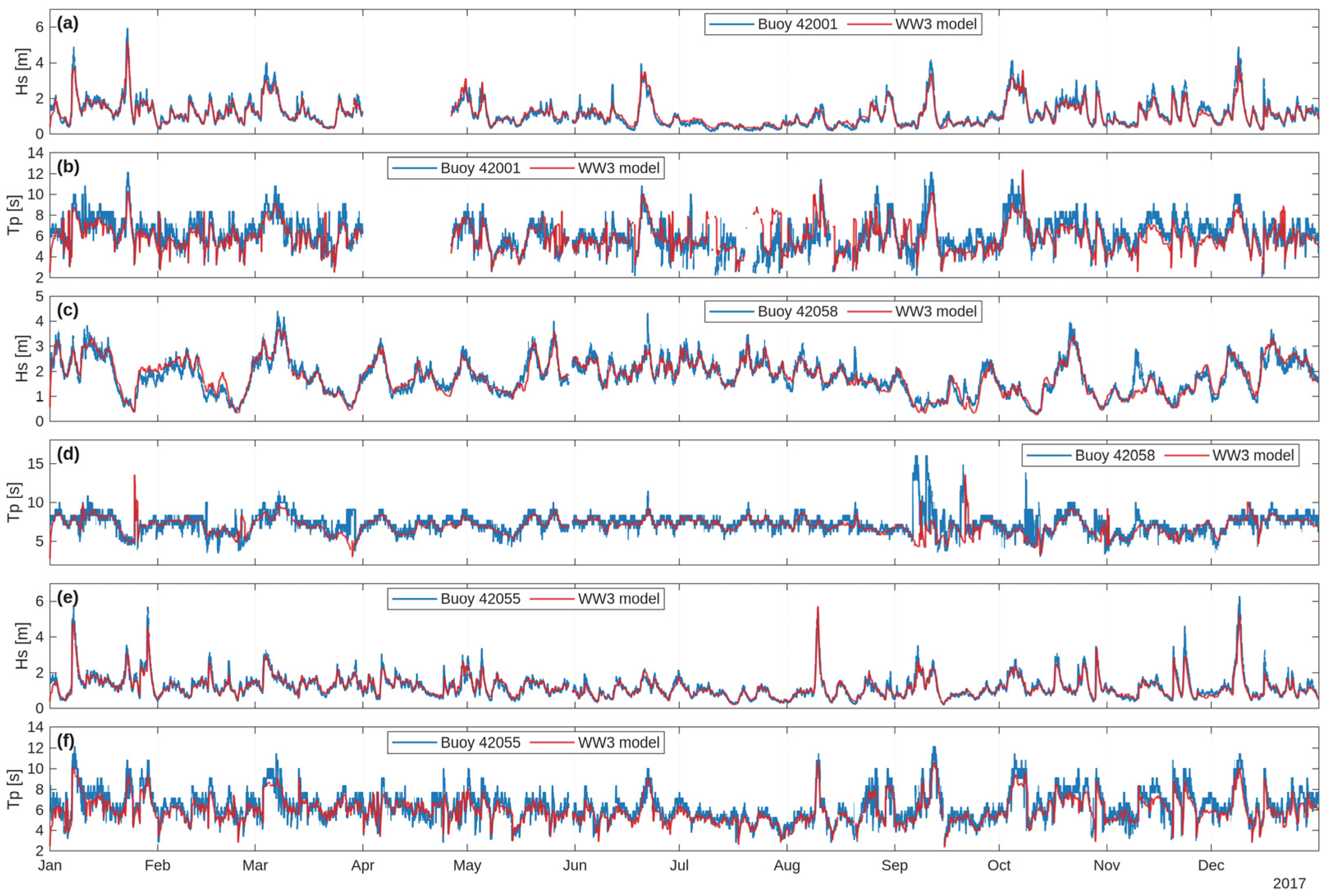
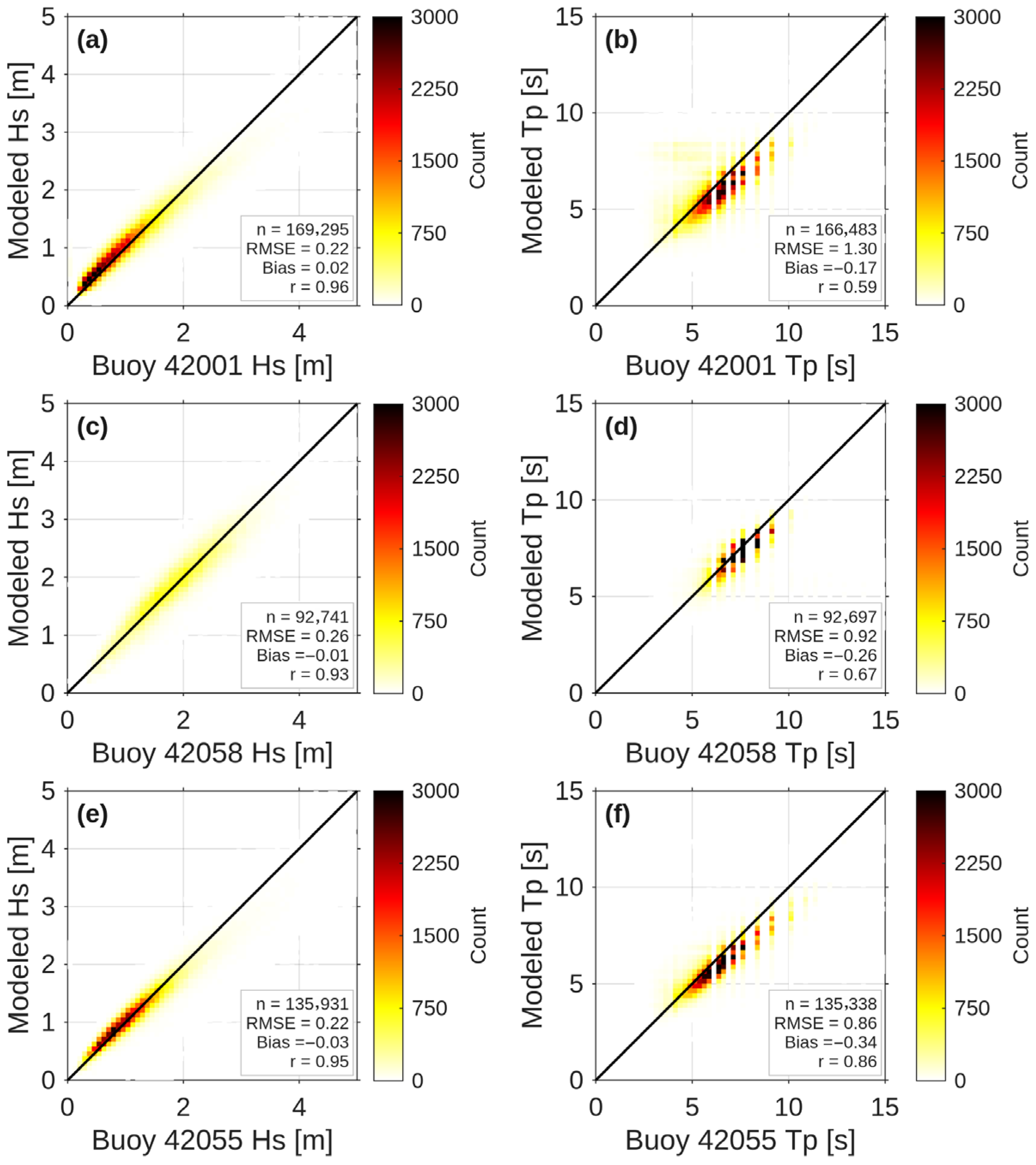
This study evaluates the performance of the WW3 model in the GoM and the Caribbean Sea using 25 years of hourly data (1998–2022) from eleven NDBC buoys. The focus is on Hs and Tp. Table 1 summarizes the location, water depth, and temporal coverage of all buoys used, while Table 2 presents the validation metrics (bias, RMSE, and CC) for each buoy. Figure 2 and Figure 3 provide deeper insights through time series and density scatter plots for buoys 42001, 42058 and 42055, which represent a range of geographic settings and performance characteristics across the study domain.
Table 1.
Location, water depth, and temporal coverage of the NDBC buoys used in this study.
Table 2.
WW3 model validation metrics for Hs and Tp based on NDBC buoys observations (1998–2022).
Figure 2.
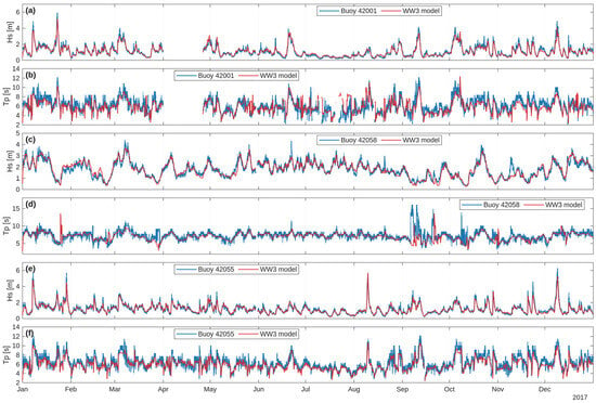
Hourly time series comparison of simulated (WW3 model) and observed wave parameters for the year 2017 at buoys 42001, 42058, and 42055: (a) Hs at buoy 42001, (b) Tp at buoy 42001, (c) Hs at buoy 42058, (d) Tp at buoy 42058, (e) Hs at buoy 42055, and (f) Tp at buoy 42055. Data gaps reflect periods of buoy unavailability.
Figure 3.
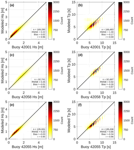
Density scatter plots comparing hourly observed (x-axis) and modeled (y-axis) Hs and Tp for the full validation period. Panels (a,b) correspond to buoy 42001, panels (c,d) correspond to buoy 42058, while panels (e,f) correspond to buoy 42055. Color scale indicates the number of data points (count) per bin. The red dashed line indicates the 1:1 agreement line between observations and model results.
As shown in Table 2, the WW3 model performs well for Hs across all eleven buoys, with RMSE values ranging from 0.17 m (buoy 42035) to 0.36 m (buoy 42059), and CC values consistently high (0.89–0.96), reflecting strong linear agreement between modeled and observed data. Bias values for Hs are generally small and near zero, indicating a slight tendency toward underprediction at some locations (e.g., −0.28 at buoy 42059) and modest overprediction at others (e.g., 0.07 m at buoy 42057). For Tp, model performance is more variable. RMSE for Tp ranges from 0.86 s (buoy 42055) to 1.30 (buoy 42001), while CC values span from 0.10 (buoys 42059) to 0.86 (buoy 42055). Buoy 42059 displays a notably low Tp correlation (CC = 0.10). A similarly low Tp correlation (CC = 0.15) was reported by Appendini et al. [13] at this same buoy using MIKE 21 [33] hindcast. The fact that two independent wave models—MIKE 21 and WW3—yield comparably poor Tp performance at this location suggests that this is not a model specific artifact, but rather reflects an inherent challenge in reproducing Tp variability at buoy 42059, likely associated with the dominant influence of Atlantic swell propagation into this sub-region, which is not fully captured within a regionally bounded model domain. The remaining buoys exhibit moderate to good Tp correlation (0.57–0.86).
Figure 2 illustrates the 2017 time series for buoys 42001 (panels a,b), 42058 (panels c,d), and 42055 (panels e,f), comparing WW3 model output against buoy observations for both Hs and Tp. For Hs, the model successfully reproduces the observed seasonal variability and short-term fluctuations, including elevated wave conditions during fall storm events. Overall agreement is strong across all three buoys, consistent with the high CC values reported in Table 2. For Tp, the model captures the general temporal evolution but exhibits larger discrepancies, particularly during periods of mixed sea states or when swell components dominate, which is reflected in the higher RMSE and, in some cases, lower CC values.
Figure 3 presents scatter plots comparing WW3 outputs with buoy observations for buoys 42001 (panels a,b), 42058 (panels c,d), and 42055 (panels e,f). For Hs (panels a,c,e), data points exhibit a high degree of clustering along the 1:1 line at all three buoys, with RMSE values of 0.22 m, 0.26 m, and 0.22 m, respectively. The bias values are 0.02 m, −0.01, and −0.03, and CC values are 0.96, 0.93, and 0.95 m, respectively. This tight clustering in indicative of the model’s reliability in reproducing Hs across a range of contrasting environments. For Tp (panels b,d,f), the scatter plots show greater dispersion, with RMSE values of 1.30 s, 0.92 s, and 0.86 s, respectively. Correspondingly, the bias values were −0.17 s, −0.26 s, and −0.34 s, while the CC values were 0.59, 0.67, and 0.86, respectively.
The WW3 model demonstrates robust performance across the GoM and the Caribbean Sea, particularly for Hs. This is evidenced by high CC and low RMSE values, which indicate reliable predictions across diverse wave conditions and over a 25-year validation period. The slight negative bias observed for Hs at several buoys suggest a systematic, modest underprediction whose specific cause was not investigated in the present study, but which may be associated with limitations in the wind forcing, wave dissipation parameterizations, or the absence of Atlantic swell at the eastern boundary of the domain, as noted in analogous studies [25]. For Tp, performance is less consistent, with larger errors and lower correlations at certain buoys, most notably buoy 42059. This is likely influenced by complex swell propagation from the Atlantic and the inherent difficulty of reproducing Tp dynamics in transitional or mixed sea states. Unlike integrated parameters such as Hs, Tp is highly sensitive to small shifts in the spectral shape between discrete frequency bins, making the spectral peak ambiguous and increasing model uncertainly. Time series of Hs and Tp for the remaining eight buoys are presented in the Appendix A (Figure A1, Figure A2 and Figure A3), and the corresponding scatter plots are shown in Figure A4, Figure A5 and Figure A6.
3.2. Trend Analysis of Mean Values
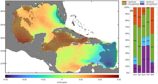
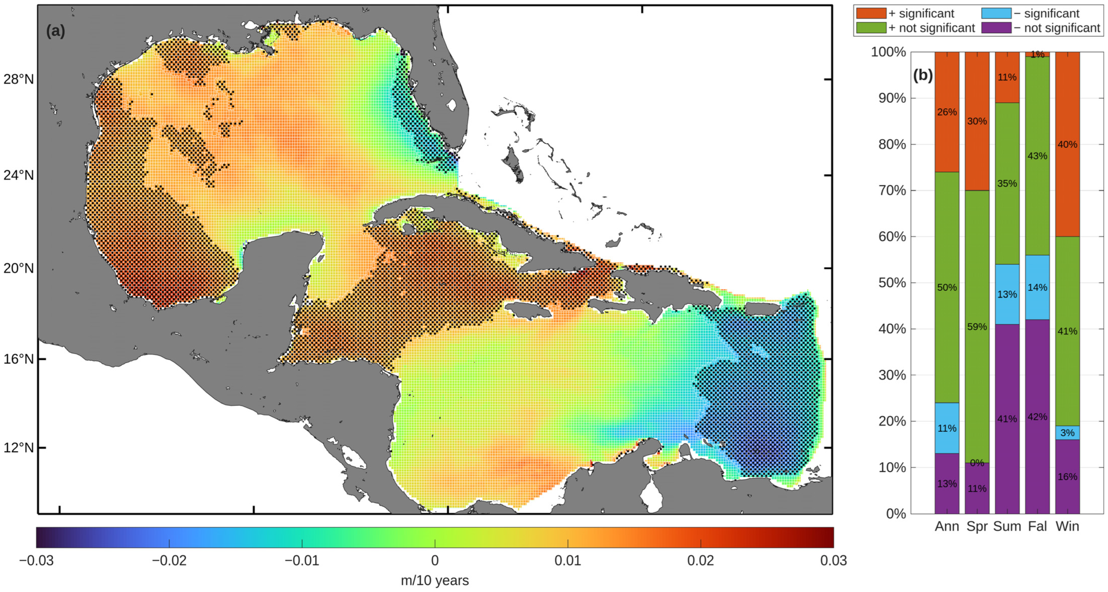
The results of the trend analysis applied to the annual and seasonal mean values of Hs are presented in Figure 4 and Figure 5. On an annual basis, a predominant positive trend is evident: 76% of the grid points exhibit increasing trends (26% statistically significant), whereas 24% show decreasing trends (11% statistically significant). These results are broadly consistent with those of Appendini et al. [13], who reported increases in mean Hs in the GoM and the Caribbean Sea at rates of up to 0.03 m/yr over the period 1979–2008, although direct comparison is limited by the difference in periods of record. Similarly, global analyses by Ahn et al. [34] (1980–2009) and Cao et al. [35] (1980–2003) indicate an overall increase in wave height in the western Atlantic over recent decades, primarily driven by an increase in surface wind speeds. The consistency of these findings across different periods and methodologies lends additional support to the positive Hs trends identified in the present study.
Figure 4.
(a) Spatial distribution of the annual trend in mean Hs. (b) Annual and seasonal percentages of grid points exhibiting positive or negative trends, including their statistical significance. The bar chart presents the percentages of grid points with positive or negative Hs trends. It should be noted that the shaded regions in the spatial trend maps (Figure 4 and subsequent figures) denote areas where the trend is statistically significant at the 95% confidence level.
Figure 5.
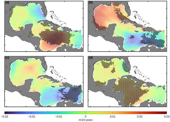
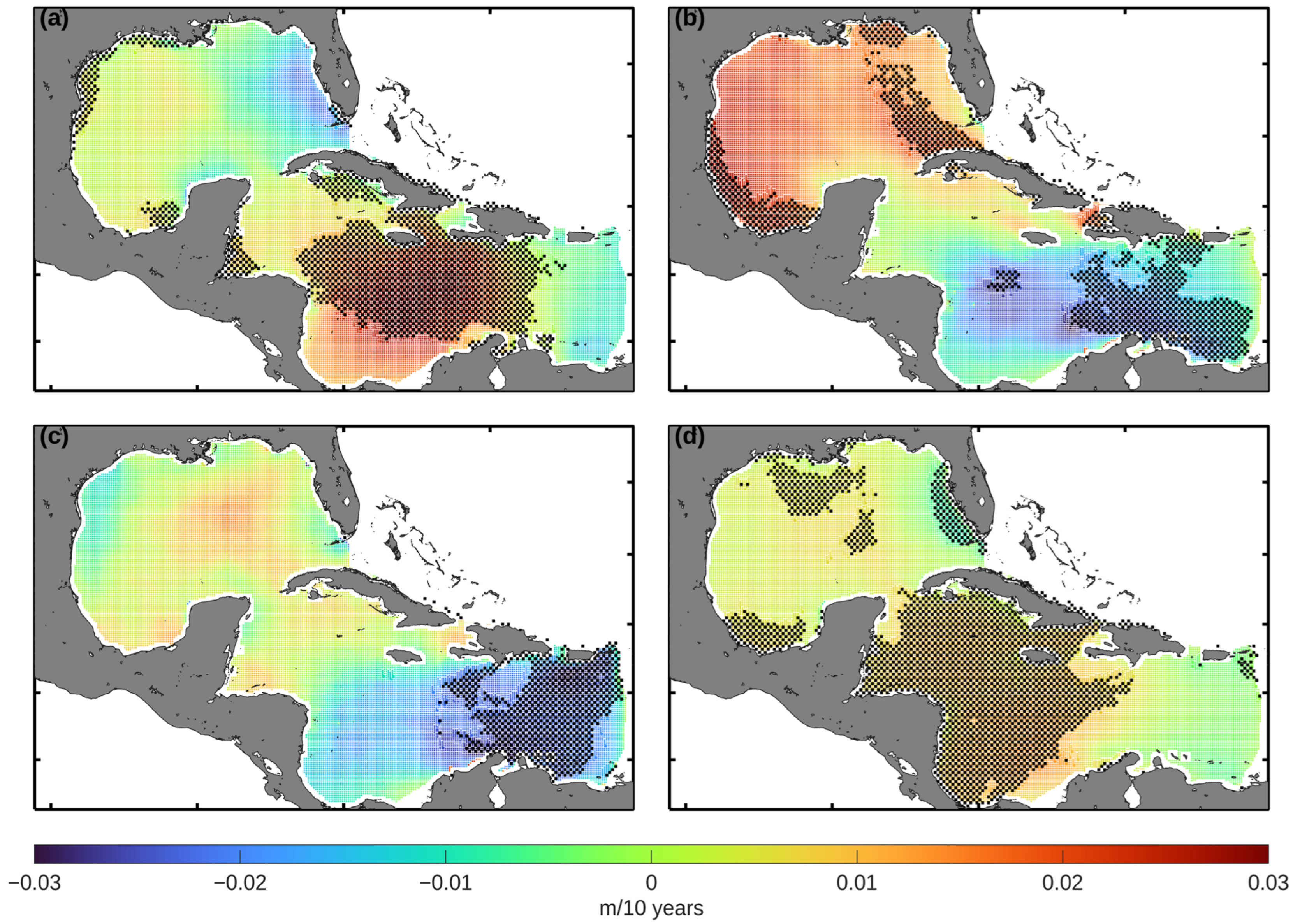
Spatial distribution of the seasonal trend in mean Hs values for (a) spring, (b) summer, (c) fall, and (d) winter.
The mean annual increase in Hs, as observed in this study, is geographically concentrated across the southwestern GoM and the Caribbean Sea, particularly between Honduras and Cuba. In contrast, the only sector with a negative annual trend is in the eastern Caribbean Sea, where the maximum decrease reaches −0.02 m/10 years (Figure 4). This negative trend may be partly associated with the absence of Atlantic swell in the model domain, as the closed eastern boundary prevents the propagation of remotely generated swell energy into this sub-region. Panchang et al. [15] have also described this pattern of localized decrease in other regions of the GoM, identifying areas with negative trends of up to −0.016 m per year in the western part of the GoM.
Seasonal definitions follow standard meteorological conventions: winter (December–February), spring (March–May), summer (June–August), and fall (September–November). The seasonal trend analysis presented in Figure 5 confirms the results derived from the annual scale, indicating a general positive trend in the mean values of Hs, although the magnitude fluctuates according to the season. In the winter months, approximately 40% of the grid points show a significant positive trend. A similar pattern is seen in spring, with around 30% of grid points demonstrating significant increases. In contrast, there is a mixture of positive and negative trends in summer and fall, with positive trends occurring in 11% and 1% of the grid points, respectively, and negative trends affecting 13% and 14%, respectively.
In spring (Figure 5a), significant positive trends exceeding 0.03 m/10 years are observed in the central Caribbean Sea, accompanied by more localized increases (0.01 m/10 years) in the GoM. In summer (see Figure 5b), the most significant increases (over 0.025 m/10 years) are seen in the western part of the GoM. Conversely, negative trends exceeding −0.02 m/10 years have been documented in the eastern Caribbean, near to the Lesser Antilles. By fall (Figure 5c), a continued decrease is seen in this region, reaching a maximum decrease of approximately −0.03 m/10 years. This seasonal pattern is broadly consistent with the findings reported by Montoya et al. [16], who noted that Hs variability in the Caribbean in summer and fall is strongly modulated by cyclonic activity and the intensification of the CLLJ over the period 1979–2012, although direct comparison is limited by the difference in periods of record. Finally, winter trends (Figure 5d) are similar to those for spring, with positive Hs trends predominating in the southern and northern regions of the GoM (>0.01 m/10 years) while, in the Caribbean Sea, there are moderate increases of up to 0.015 m/10 years.
These changes in the regional wave climate may have practical implications for a variety of maritime and offshore activities in the GoM and the Caribbean Sea. An increasing trend in Hs could influence the operational conditions along major maritime shipping corridors. These corridors are used by container and cargo vessels connecting the Panama Canal, the Caribbean basin, and the northern Gulf ports. Higher wave conditions have been shown to affect vessel routing, transit times, and navigational safety, particularly during extreme sea states, which are known to pose risks to commercial shipping and offshore operations [36,37]. Furthermore, variations in wave climate are relevant to offshore oil and gas operations. More energetic wave conditions may increase operational hazards and affect the transport and dispersion of oil in the event of accidental spills [38].
The trend analysis of wave period is presented in terms of energy period rather than the Tp, for two main reasons. First, Te is more directly relevant to wave energy resource assessment, as it better represents the energy content of the wave spectrum. Second, since Te is derived from Tp through the relationship , the validation of Tp presented in Section 3.1 serves as an indirect validation of Te, and the accuracy of Te estimates can be considered consistent with that of Tp across the study domain.
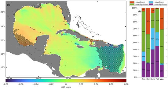
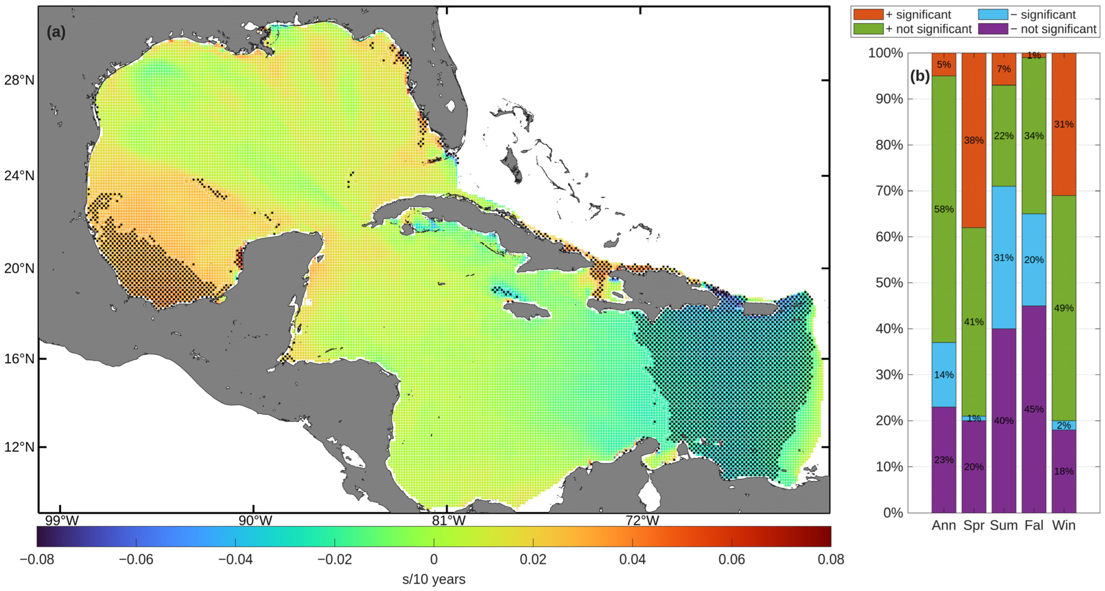
Figure 6 presents the trend analysis of annual and seasonal mean Te values. A pronounced positive trend is evident on an annual basis, as well as during the spring and winter months. The proportion of grid points with a significant positive trend remains modest, with 38% in spring, 7% in summer, 1% in fall, and 31% in winter. The spatial pattern for the annual mean of Te indicates isolated positive trends in the western GoM, reaching up to 0.03 s/10 years, while an area in the eastern Caribbean Sea displays a decreasing trend of about −0.04 s/10 years.
Figure 6.
(a) Spatial distribution of the annual trend in mean Te. (b) Annual and seasonal percentages of grid points exhibiting positive or negative trends, including their statistical significance.
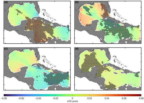
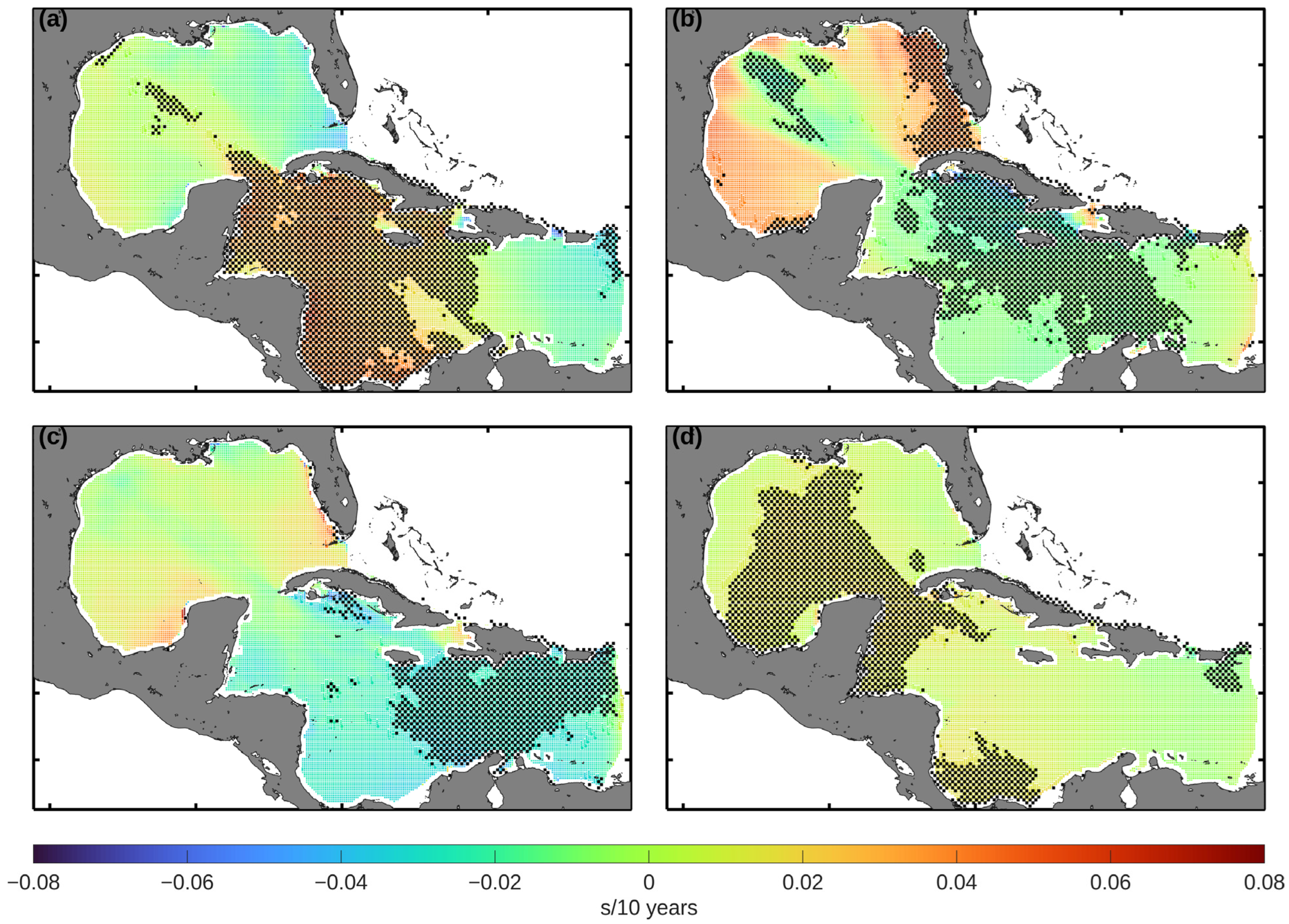
Figure 7 shows the spatial distribution of seasonal Te trends in the GoM and the Caribbean Sea. In spring (Figure 7a), there is a positive Te trend throughout the Caribbean Sea, with maximum values exceeding 0.04 s/10 years. However, in a comparatively smaller area of the central GoM there is a weak negative trend, with a value of approximately −0.02 s/10 years. The summer pattern (Figure 7b) shows a similar trend, although negative trends intensify to approximately −0.03 s/10 years in the central Caribbean Sea. In the fall months (Figure 7c), negative trends predominate in the eastern Caribbean Sea, with a recorded decrease of −0.04 s/10 years. In winter (Figure 7d), the overall pattern remains consistent, with positive trends in the central GoM, peaking at almost 0.01 s/10 years.
Figure 7.
Spatial distribution of the seasonal trend in mean Te values for (a) spring, (b) summer, (c) fall, and (d) winter.
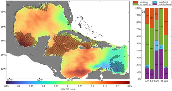
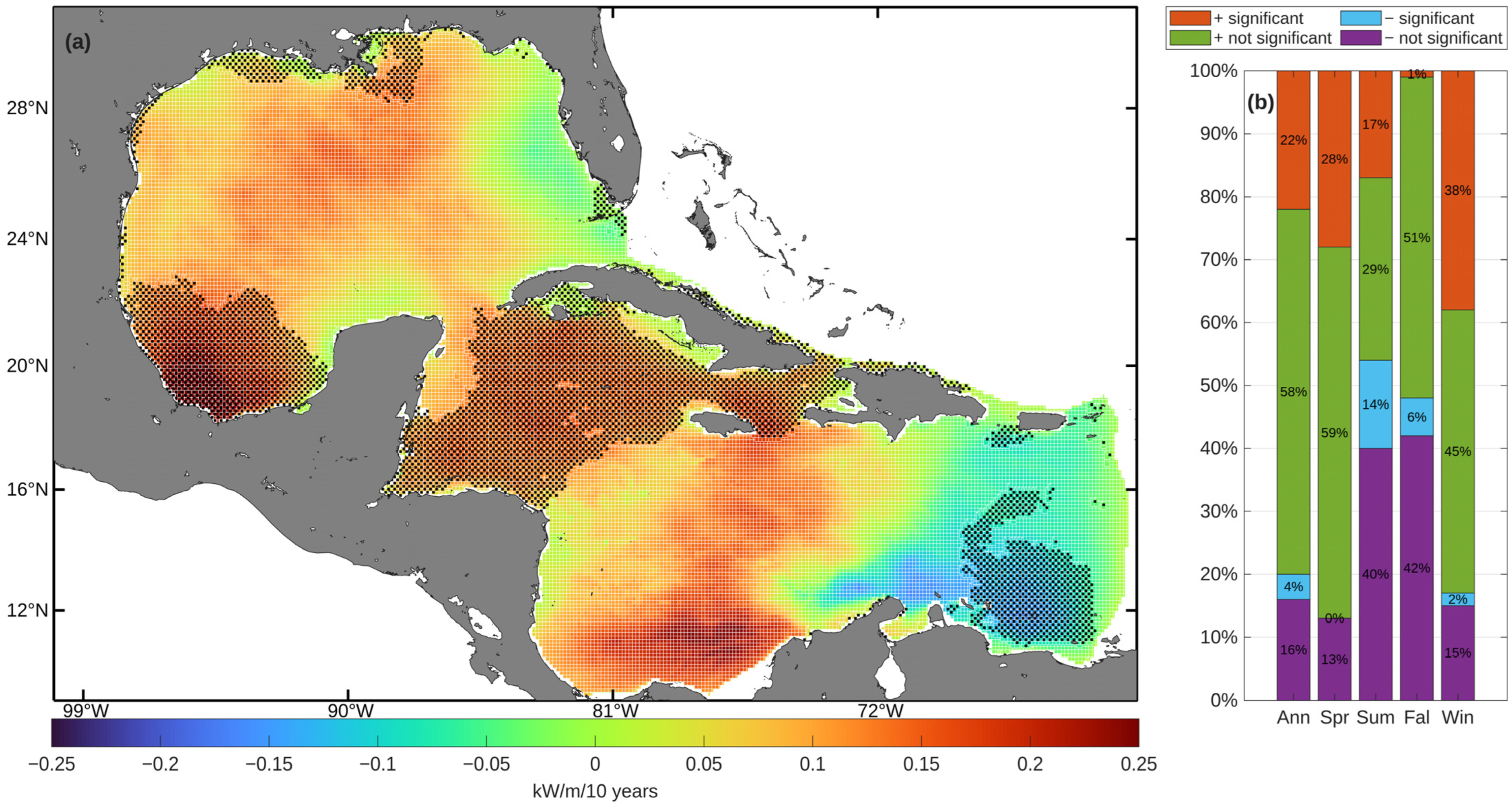
Figure 8 and Figure 9 present the results of the trend analysis applied to annual and seasonal mean P values in the Caribbean and the GoM. The annual dataset reveals a predominantly positive trend: 80% of the grid points exhibit increasing trends (22% statistically significant), whereas 20% show decreasing trends (4% statistically significant). Figure 8 shows that most nodes exhibit positive trends, reaching a maximum of 0.25 kW/m/10 years in the southwestern GoM, and approaching 0.20 kW/m/10 years in the Caribbean Sea. Negative trends have been observed primarily in the eastern Caribbean, around the Lesser Antilles, with a minimum recorded value of −0.15 kW/m/10 years. A significant positive trend was observed in 28% of the nodes in spring, 17% in summer, 1% in fall, and 38% in winter. A total of 14% of the nodes exhibited significant negative trends in summer months, 6% in fall, and 2% in winter.
Figure 8.
(a) Spatial distribution of the annual trend in mean P. (b) Annual and seasonal percentages of grid points exhibiting positive or negative trends, including their statistical significance.
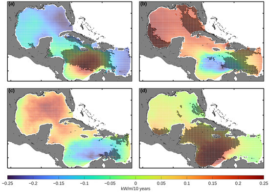
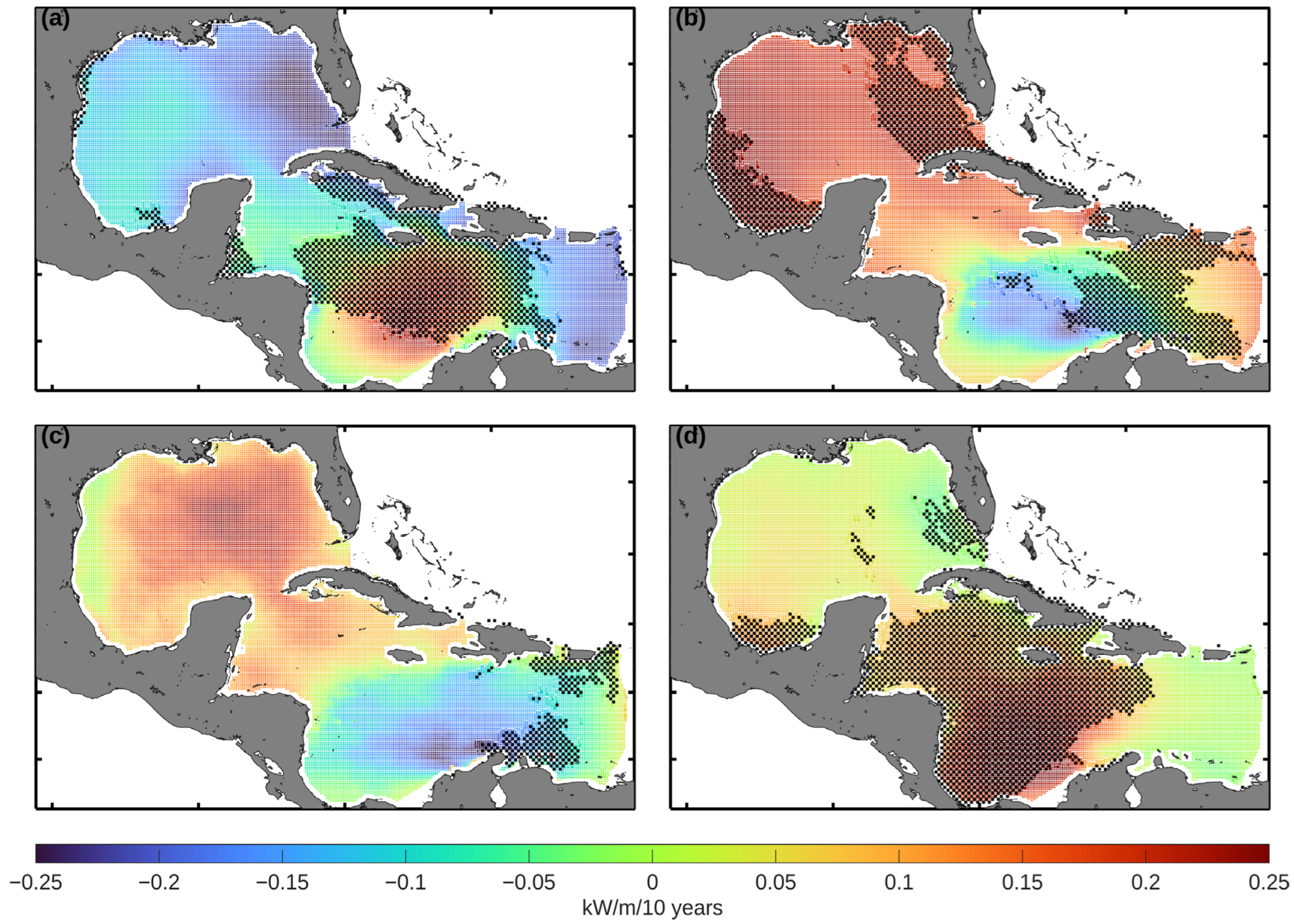
Figure 9.
Spatial distribution of the seasonal trends of mean P values for (a) spring, (b) summer, (c) fall, and (d) winter.
There is a marked spatial contrast between the four seasons. In spring (Figure 9a), positive trends predominate, reaching approximately 0.25 kW/m/10 years, with a concentration in the central Caribbean. Similarly, the summer months (Figure 9b) exhibit positive trends of up to 0.20 kW/m/10 years near Florida and the southwestern GoM. Conversely, isolated negative trends as low as −0.10 kW/m/10 years occur west of the Lesser Antilles. As illustrated in Figure 9c, the fall months are characterized by negative trends across most of the eastern Caribbean, with the minimum reaching approximately −0.15 kW/m/10 years. In winter (Figure 9d), the strongest positive trends reappear in the central Caribbean Sea, with values ranging from 0.15 to 0.25 kW/m/10 years. These P patterns closely mirror the Hs distributions documented in Figure 4 and Figure 5, which is expected given that P scales with the square of Hs and linearly with Te in the deep-water approximation (Equation (4)).
From the perspective of renewable energy, the observed trends in P could determine the positioning of offshore wind farms by defining the metocean conditions they must withstand, while directly influencing the potential for wave energy exploitation. Regions experiencing increasing wave heights may have enhanced wave energy potential for wave energy converters, although greater wave variability could also impose more stringent constraints on the design and operation of marine energy infrastructure [39,40].
Our analysis identifies a marked seasonal difference in wave climate trends across the GoM and the Caribbean Sea. The most robust signal is a significant intensification of Hs and P during winter and spring, with a high percentage of grid points showing significant positive trends (40% for Hs and 38% for P in winter). This phenomenon aligns with a hypothesized strengthening of mid-latitude frontal systems and extratropical storm tracks. In contrast, summer and fall are characterized by a predominant signal of negative trends, most notably in Te, where over a third of the domain exhibits decreasing tendencies. The decreasing Te trends observed in the eastern Caribbean Sea should be interpreted with caution, as they may be partly associated with the absence of Atlantic swell in the model domain. Significant negative trends become conspicuous in these seasons, especially for Te (31% in summer) and Hs (13%). This seasonal contrast suggests the presence of distinct climatic drivers: winter/spring trends are likely associated with large-scale atmospheric circulation from cold fronts, while summer/fall trends may be influenced by changes in tropical cyclone trajectories, trade wind intensity, or local wind–sea processes. These factors are supported by the alignment of seasonal peaks with the Atlantic tropical cyclones season and the island-induced sheltering observed in the eastern Caribbean.
The annual mean trends, which demonstrate a net positive increase in wave energy, obscure this substantial intra-annual variability. Consequently, coastal systems are not undergoing uniform change; rather, they are experiencing a sharpening of the seasonal cycle. This implies heightened erosion risk during already energetic winters, and a shift in spectral wave climate during calmer summers.
3.3. Correlation with Climate Indices
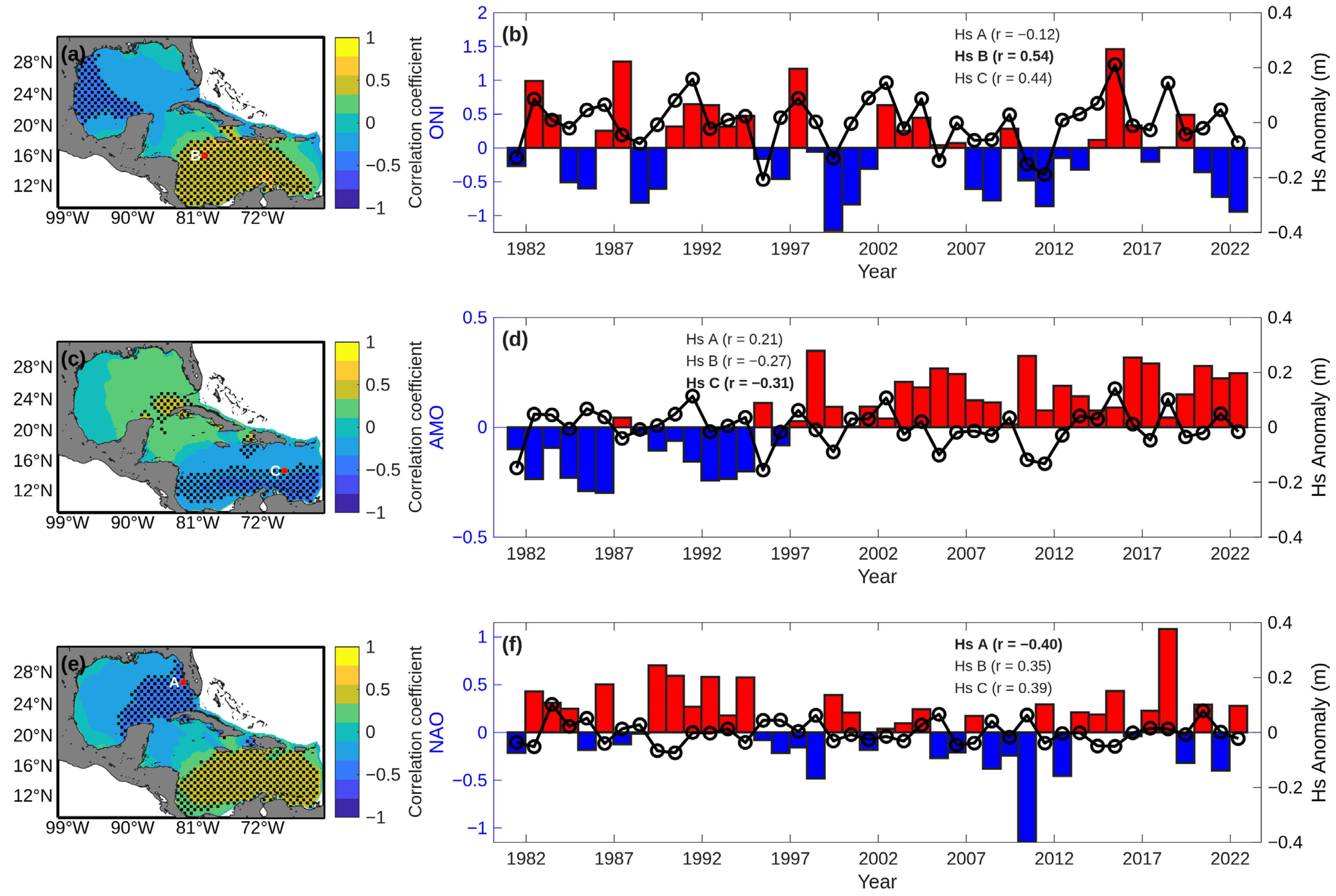
Following the identification of spatio-temporal patterns in wave parameter trends, we explore the underlying climatic mechanisms modulating this variability. We examine the relationships between annual anomalies of Hs, Te, and P—derived from hourly WW3 model estimates aggregated to annual means—and three large-scale climate indices relevant to the North Atlantic and tropical dynamics: the ONI, the AMO index, and the NAO index. The objective is to assess how low-frequency climate modes influence interannual wave climate fluctuations, and to what extent regional trends are driven by these teleconnections versus local processes. To this end, three representative locations (Points A, B, and C; Figure 10) were selected based on the spatial trend analysis, corresponding to areas that exhibited statically significant trends in Hs, Te, or P. Point is located in the Gulf of Mexico, while Points B and C are situated in the Caribbean Sea, providing spatial coverage across both basins of the study domain. For each location, annual anomalies of the wave parameters were correlated with the corresponding climate indices, and the location with the highest correlation is highlighted in the figures.
Figure 10.
Spatial and temporal correlations between annual Hs anomalies and climate indices (ONI, AMO, and NAO) in the GoM and the Caribbean Sea. Panels (a,c,e) show the spatial distribution of correlation coefficients between Hs anomalies and ONI, AMO, and NAO, respectively; the stippling indicates statistically significant regions (p < 0.05). Panels (b,d,f) show the time series of annual Hs anomalies (black line with open circles indicating individual annual values) for the location among the three analyzed (A, B, or C) that yielded the highest correlation with the respective climate index (bars). Red bars indicate positive index anomalies, while blue bars indicate negative index anomalies. Correlation coefficients (r) for all three points are provided in the legends, with the maximum values highlighted in bold.
Figure 10 reveals a distinct contrast in the response to ENSO between the GoM and the Caribbean Sea. Positive correlations exceeding 0.50 are observed in the central Caribbean, suggesting an increase in Hs during El Niño conditions. Conversely, the western Caribbean and extensive portions of the GoM exhibit moderate to strong negative correlations (locally reaching r < −0.40), characterizing a dipolar spatial structure. Time series comparisons (Figure 10b) indicate coherent interannual variability between ONI and Hs anomalies (r = 0.54), with notable positive Hs responses during the 1982–83, 1997–98, and 2015–16 extreme El Niño events.
This dipole pattern is indicative of ENSO-related modulation of regional atmospheric circulation. During El Niño events, anomalous convective heating in the equatorial Pacific triggers teleconnections that alter the CLLJ. Observational and modeling studies indicate that El Niño is typically associated with a weakened CLLJ and reduced trade wind intensity over the western Caribbean, thereby limiting local wind-wave generation [41]. Conversely, shifts in the position of the Intertropical Convergence Zone (ITCZ) and enhanced upper-level divergence over the central and eastern Caribbean favors increased forcing in those sectors [42].
The AMO exhibits a distinct but weak relationship with Hs, characterized by negative correlations (r ≈ −0.31) localized in the southern Caribbean (Figure 10c,d). Warm AMO phases, associated with elevated North Atlantic sea surface temperatures (SSTs), coincide with slight reductions in significant wave height in these areas. Compared to ENSO, the AMO signal is less pronounced, which is consistent with its primary role in shaping basin-scale SST variability and long-term ocean–atmosphere interactions, rather than exerting strong control on regional wind fields [31]. It should be noted that Point C is located in the eastern Caribbean Sea, where the absence of Atlantic swell due to the closed model boundary may influence the wave climate estimates, and therefore the results at this location should be interpreted with caution. These results suggest that the contribution of the AMO to Hs variability within the study domain is modest.
In contrast, the NAO has a more robust relationship with Hs, featuring positive correlations in the central and eastern Caribbean Sea, with values reaching (r = 0.39) (Figure 10e). Conversely, moderate negative correlations (r ≈ −0.40) are observed over the northeastern GoM, where the highest correlation among the three analyzed points was r = −0.40 (Figure 10f). In positive NAO phases, the intensified subtropical high and the poleward shift in the Atlantic storm track [32] tend to suppress the influence of mid-latitude disturbances in the GoM, thereby reducing wave activity. Under negative NAO conditions, the southward displacement of the storm track allows for greater penetration of extratropical systems into the GoM, favoring increased wave generation. Similar storm-track-driven modulations of the wave climate associated with the NAO have been documented in the Northeast Atlantic [43].
Moderate correlation values between wave climate variables and large-scale climate indices are expected and consistent with the literature, as climate indices represent basin-scale atmospheric variability that only partially explains local wave conditions. Local wave regimes are additionally modulated by wind forcing, storm tracks, and regional oceanographic factors. For instance, Maia et al. [44] reported maximum correlations of approximately 0.65 between wave parameters and climate indices AMO, the Tropical Southern Atlantic Index (TSA), and the Southern Annular Mode (SAM) in the South Atlantic Ocean, which are comparable to the values obtained in the present study.
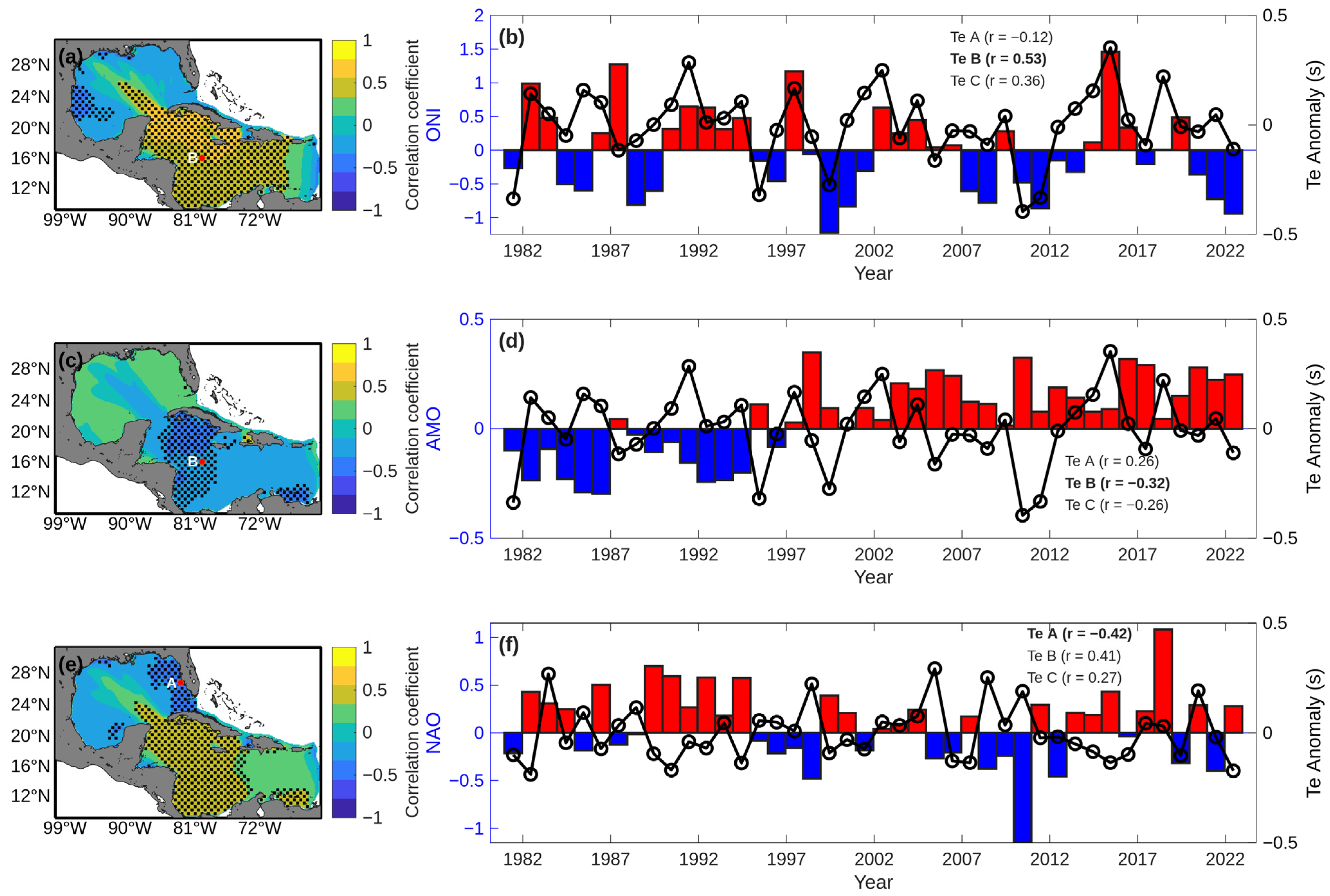
Figure 11a shows that Te presents the most spatially coherent climate-related signal among the wave parameters analyzed. Positive correlations with the ONI dominate the central and eastern Caribbean (maximum r = 0.53), suggesting an increase in Te during El Niño events. This relationship is further evidenced in the time series (Figure 11b), which shows a strong positive coupling between the ONI and Te. This pattern is consistent with a greater influence of remotely generated swell under altered large-scale circulation conditions [45]. Conversely, negative correlations observed in the western Caribbean and the GoM point to a reduced contribution of locally generated sea-wind during periods of weakened trade winds.
Figure 11.
Spatial and temporal correlations between annual Te anomalies and climate indices (ONI, AMO, and NAO) in the GoM and the Caribbean Sea. Panels (a,c,e) show the spatial distribution of correlation coefficients between Te anomalies and ONI, AMO, and NAO, respectively; the stippling indicates statistically significant regions (p < 0.05). Panels (b,d,f) display the time series of annual Te anomalies (black line with open circles indicating individual annual values) for the location among the three analyzed (A, B, or C) that yielded the highest correlation with the respective climate index (bars). Red bars indicate positive index anomalies, while blue bars indicate negative index anomalies. Correlation coefficients (r) for all three points are provided in the legends, with the maximum values highlighted in bold.
Negative correlations between the AMO and Te dominate much of the basin (r ≈ −0.30), particularly in the southern Caribbean (Figure 11c). The selected time series (Figure 11d) further illustrates this negative coupling (r = −0.32), indicating a tendency toward shorter wave periods in warm AMO phases. Such behavior is consistent with the increase in trade wind forcing associated with strengthened meridional SST gradients [46], as well as with potential shifts in North Atlantic storm tracks that modulate the arrival of remotely generated swell into the Caribbean basin.
Moderate positive correlations between the NAO and Te (r ≈ 0.40) are observed in the southern basin, albeit with considerable spatial variability (Figure 11e). However, of the three representative locations, Point A had a distinct negative correlation (r = −0.42). These correlations suggest an increased influence of long-period swell during positive NAO phases for most of the Caribbean Sea. In contrast, local wave conditions in specific sectors, such as the northern GoM (Point A), respond differently due to concurrent shifts in the North Atlantic storm-track position, which can inhibit or enhance the arrival of extratropical swell.
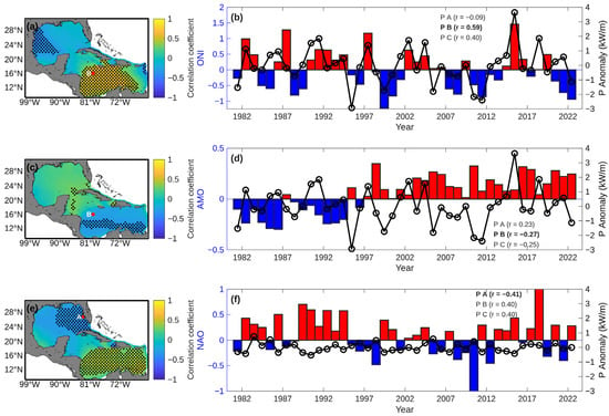
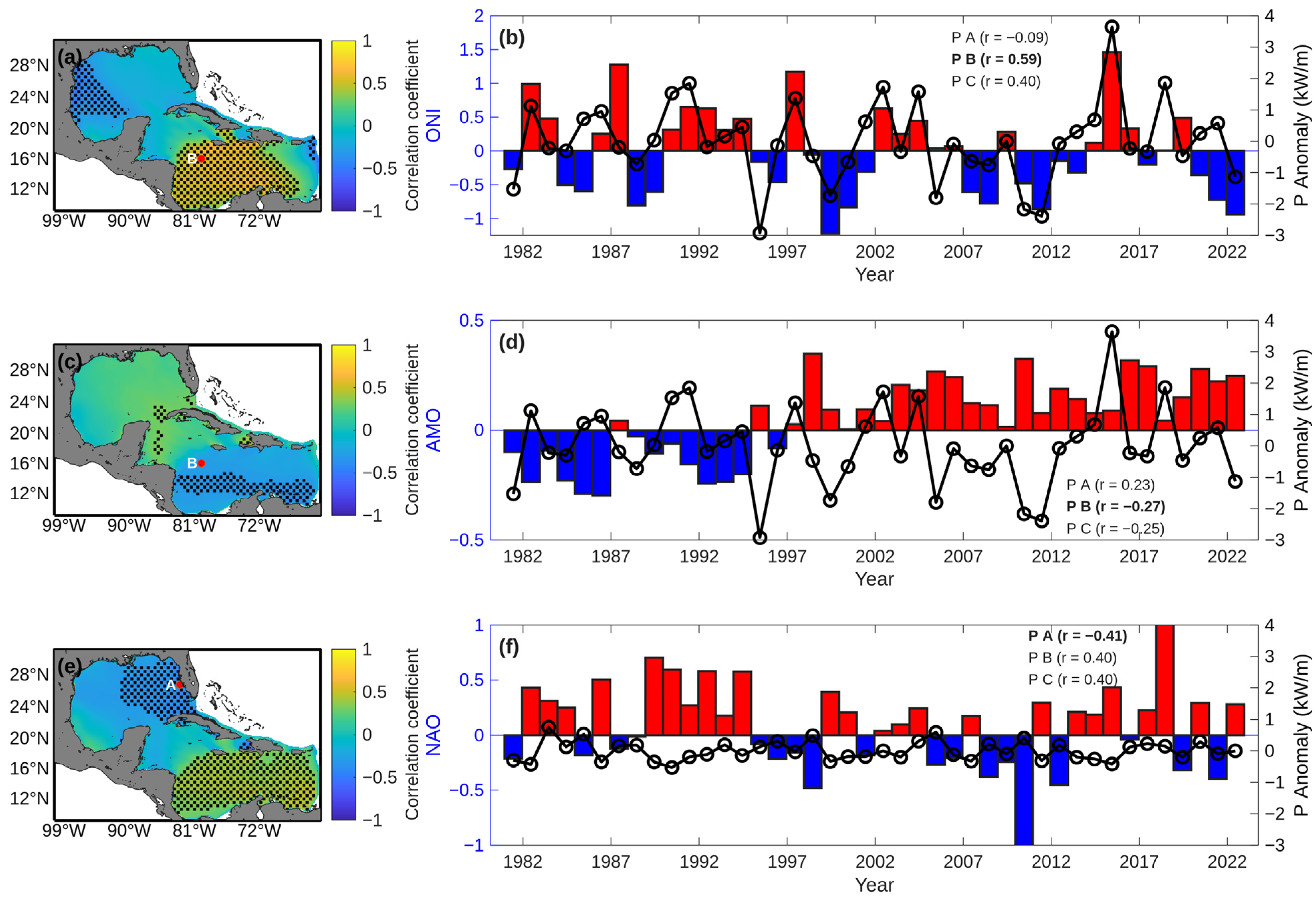
Since P depends on both and Te, its spatial patterns of climate variability are expected to broadly reflect those of Hs, while the linear contribution of Te may introduce additional modulation in regions where wave period variability is particularly pronounced. Strong positive correlations with the ONI are observed in the central Caribbean Sea (r > 0.50), suggesting enhanced wave energy flux during El Niño conditions (Figure 12a). The corresponding time series (Figure 12b) shows the strongest correlation among all studied variables with ONI, reaching r = 0.59. Conversely, negative correlations in the northwestern GoM (r ≈ −0.45) result in a clear dipolar response across the study domain.
Figure 12.
Spatial and temporal correlations between annual P anomalies and climate indices (ONI, AMO, and NAO) in the GoM and the Caribbean Sea. Panels (a,c,e) show the spatial distribution of correlation coefficients between P anomalies and ONI, AMO, and NAO, respectively; the stippling indicates statistically significant regions (p < 0.05). Panels (b,d,f) show the time series of annual P anomalies (black line with open circles indicating individual annual values) for the location among the three analyzed (A, B, or C) that yielded the highest correlation with the respective climate index (bars). Red bars indicate positive index anomalies, while blue bars indicate negative index anomalies. Correlation coefficients (r) for all three points are provided in the legends, with the maximum values highlighted in bold.
The relationship between the AMO and P is weak, with statistically significant correlations confined to localized areas (Figure 12c,d). Negative correlations are seen in parts of the central Caribbean, whereas a small area near the Yucatán Channel has positive correlations. The representative time series at Point B further reflects this weak association (r = −0.27). These results indicate that the contribution of AMO to P variability is minor compared to other climate modes, consistent with its primary influence on basin-scale thermal structures. Unlike ENSO-driven variability, AMO-related signals lack basin-wide spatial coherence in the study domain.
The NAO exhibits a spatially heterogeneous influence on wave power (Figure 12e,f). Strong positive correlations dominate the central and eastern Caribbean (r > 0.50), indicating enhanced wave energy flux during positive NAO phases. Conversely, a distinct region west of Florida, in the GoM, has negative correlations, with Point A showing a moderate inverse relationship (r = −0.41).
The spatial analysis reveals that ENSO is the dominant driver of interannual wave climate variability across the Caribbean–GoM system, whereas the NAO exerts regionally dependent control, and the AMO plays a secondary, multidecadal role.
Trend–Teleconnection Interaction Analysis
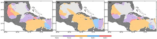
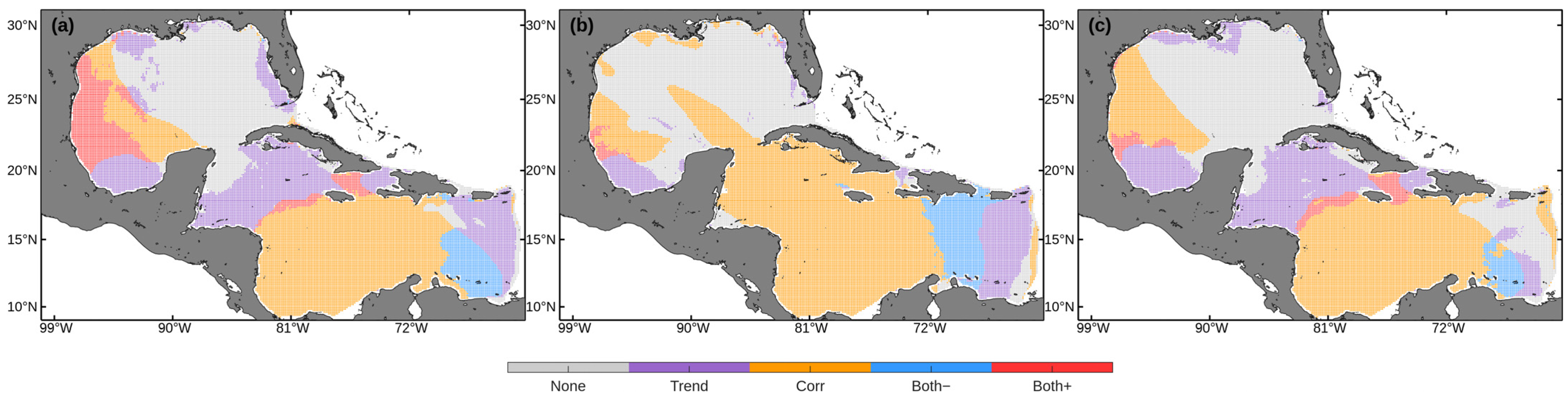
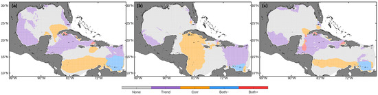
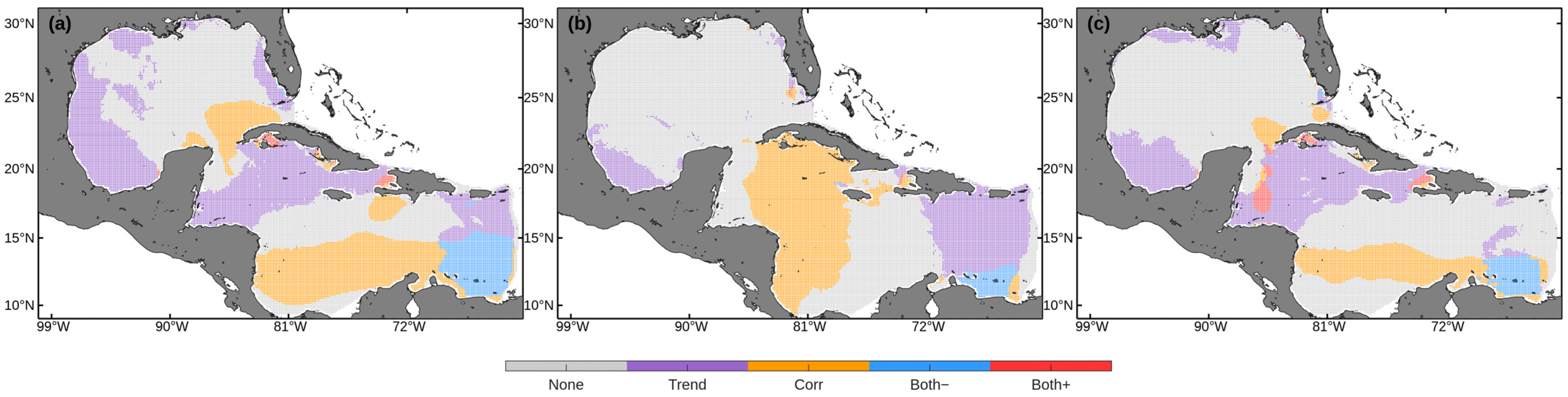
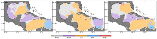
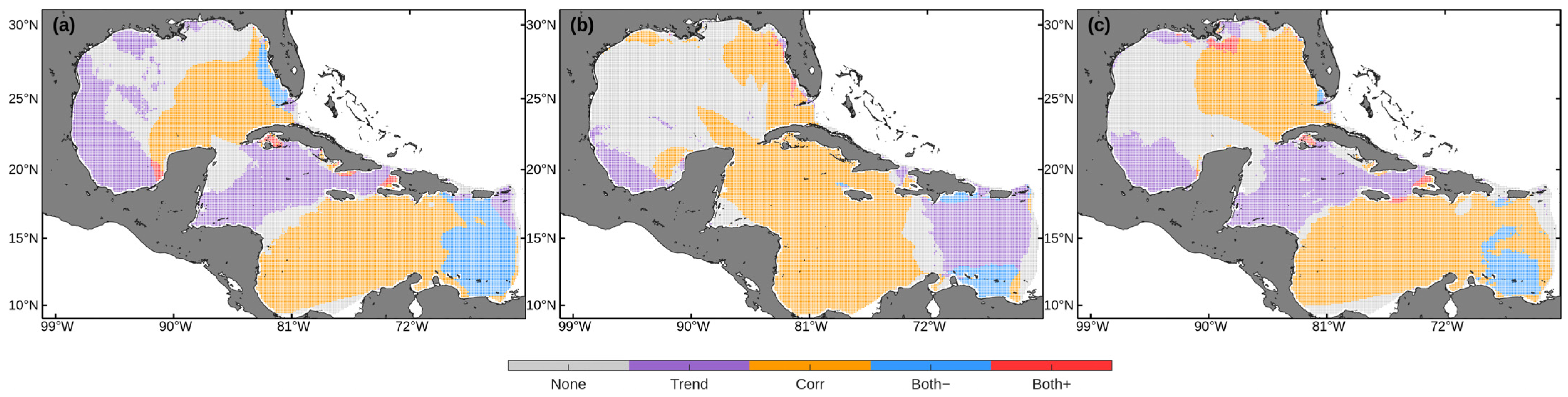
Figure 13, Figure 14 and Figure 15 overlay long-term linear trends with climate correlations, revealing distinct spatial patterns in the interaction between interannual variability and multidecadal change. Each grid point is classified into five categories: “None” (neither trend nor correlation significant), “Trend” (significant trend only), “Corr” (significant correlation only), “Both+” (positive trend with significant correlation), and “Both−” (negative trend with significant correlation). Significance correlation was determined using a two-tailed Pearson correlation test (p < 0.05), equivalent to |r| > 0.304 for n = 42 annual values.
Figure 13.
Spatial distribution of trends in (a) Hs, (b) Te, and (c) P overlaid with their respective correlations with the ONI.
Figure 14.
Spatial distribution of trends in (a) Hs, (b) Te, and (c) P overlaid with their respective correlations with the AMO index.
Figure 15.
Spatial distribution of trends in (a) Hs, (b) Te, and (c) P overlaid with their respective correlations with the NAO index.
Regarding Hs, the Caribbean has greater sensitivity to ENSO than the GoM. There are significant correlations with the ONI in approximately 40% of the Caribbean domain, with a notable co-occurrence of negative trends (“Both−”) in the eastern Caribbean Sea (Figure 13a). These “Both−” regions are noteworthy as they identify areas where declining long-term trends coincide with strong ENSO-related variability. This alignment suggests that the observed multidecadal decrease in Hs may be partially influenced by the cumulative effect of ENSO phase variability in the period of analysis [47].
In contrast, in the GoM ENSO-related correlations are only seen along a narrow band extending from the Yucatán Peninsula toward the Texas coast, with less than 15% of the basin having statistically significant associations with the ONI. Within this region, a localized area of Tamaulipas and Veracruz is classified as “Both+”, indicating that ENSO variability aligns with a positive long-term trend in Hs. Despite this localized response, the overall pattern confirms that the long-term evolution of Hs in the GoM is primarily governed by regional atmospheric processes.
Te exhibits the most prominent ENSO imprint among the wave parameters analyzed (Figure 13b), with approximately 60% of the Caribbean domain showing significant correlations with the ONI. This contrast between the robust ENSO signal in Te and the more spatially limited response in Hs indicates that ENSO primarily modulates the spectral characteristics of waves through shifts in remotely generated swell, rather than through local wind–sea height variability. The underlying mechanism likely involves ENSO-induced shifts in North Pacific and North Atlantic storm tracks, which alter the characteristics and pathways of swell propagating into the Caribbean [48]. In contrast, the GoM remains insensitive to ENSO forcing, with more than 50% of the basin classified as “None” or “Trend”, underscoring the dominance of local wind–sea processes over remote swell influence.
For P, the spatial pattern reflects an intermediate response between Hs and Te (Figure 13c), integrating sensitivity to climate variability with strong regional modulation. Substantial parts of the Caribbean are dominated by “Corr” and localized areas of “Both-“ and “Both+” classifications, indicating that interannual climate forcing significantly modulates wave power. This pattern is especially evident in the central and eastern Caribbean, where the energetic contribution of remotely generated swell plays a substantial role in shaping wave power variability. Conversely, the GoM is characterized primarily by “Trend” and “None” classifications, highlighting the dominance of regional atmospheric forcing on wave power evolution. A small area in the eastern GoM, near the Yucatán Channel, has significant correlations, suggesting limited penetration of large-scale climate signals into the basin.
The AMO exerts most discernible influence in the swell-exposed sectors of the basin. For Hs, AMO-related variability is evident over some parts of the Caribbean, particularly in the central–western area, where scattered “Corr” classifications indicate sensitivity to multidecadal Atlantic variability in areas historically influenced by North Atlantic swell [12]. Nevertheless, large areas remain dominated by “Trend” or “None” categories, highlighting a heterogeneous response. In the GoM, less than 20% of the basin exhibits significant AMO correlations, while “Trend” classifications exceed 50%, reinforcing that long-term variability in wave height in the Gulf is primarily driven by regional atmospheric processes, rather than basin-scale AMO modulation (Figure 14a).
Te exhibits the clearest AMO imprint among the analyzed parameters (Figure 14b), with approximately 30% of the Caribbean displaying significant correlations. This pattern is consistent with the AMO’s documented influence on North Atlantic storminess and swell generation at multidecadal timescales [49]. In contrast, the northern GoM is dominated by “None” and “Trend” classifications (>85%).
For P, the spatial distribution reveals a hybrid but spatially constrained response to the AMO (Figure 13c). The “Both−” and “Both+” classifications occupy a limited fraction of the domain (roughly 10–20%), primarily concentrated in the central Caribbean and along the Yucatán–Cuba corridor, where preferential swell penetration pathways exist. This distribution indicates that AMO-related variability influences long-term wave energy only where persistent trends align with multidecadal Atlantic forcing. Elsewhere, particularly in the GoM, the dominance of “None” (>70%) confirms that the AMO plays a minimal role in modulating P.
For Hs, NAO-related signals are concentrated along the northern and eastern margins of the domain, with grid points predominantly classified as “Corr” (~25%) and “Both−” (~8%). In contrast, the western GoM is dominated by “None” (~35%) and “Trend” (~32%) categories, indicating that local wind–sea processes limit the sensitivity of Hs to NAO variability (Figure 15a).
Te shows a broader NAO footprint, with “Corr” classifications spanning roughly 45% of the central and southern Caribbean (Figure 15b). This pattern suggests NAO-driven modulation of swell spectral characteristics, consistent with enhanced mid-latitude westerlies during positive NAO phases that favor the generation and propagation of longer-period waves from the North Atlantic [43]. In the GoM, the “None” (~28%) and “Trend” (~30%) classifications remain prevalent, supporting a relatively weak influence of remotely generated swell on Te.
Regarding P, classifications occur sporadically in the southeastern Caribbean, indicating a localized, phase-dependent interaction between NAO variability and long-term trends. In the GoM, the high percentage of “Corr” (~48%) alongside “Trend” dominance (~17%) suggests that while wave power is sensitive to the NAO, long-term evolution is still heavily influenced by regional processes (Figure 15c).
This overlay analysis highlights a clear regional contrast between the Caribbean Sea and the GoM. In the Caribbean, approximately 25–50% of the domain shows significant correlations with at least one climate index, indicating a climate-sensitive wave regime shaped by the convergence of local forcing, remote swell, and teleconnection-driven variability. The 10–25% classified as “Both+” identifies areas where climate variability may reinforce or counteract long-term trends, which is relevant for coastal and offshore risk assessments. In contrast, the GoM is largely trend-dominated, with more than 50% of the basin showing limited sensitivity to ENSO, AMO, and NAO. This is consistent with wave conditions primarily controlled by regional processes such as cold fronts and tropical cyclones. Finally, the extensive “None” category in the central GoM suggests regions where interannual variability dominates without a robust trend or teleconnection signal, pointing to additional drivers beyond large-scale climate indices.
The trends identified in this study, particularly the predominant increase in Hs and P in the southwestern GoM and central Caribbean, are consistent with broader observations of wave climate intensification in the North Atlantic. Although our results indicate localized increases of up to 0.03 m/10 years, they are consistent with the findings of Young and Ribal [50], who reported a global upward trend in Hs, particularly in the Atlantic basin, driven by strengthening oceanic winds.
Within the region, the contrast between the eastern Caribbean (decreasing trends) and the western Caribbean (increasing trends) corresponds to the spatial variability described by Izaguirre et al. [51], who attributed such patterns to shifts in the position of the North Atlantic subtropical high.
A comparison with other ocean basins indicates that the magnitude of change in the GoM and Caribbean is more moderate than in regions such as the Southern Ocean or the North Pacific, where some of the strongest increases in wave height have been reported globally [10,50]. However, the dynamic importance of the Caribbean as a transition zone for swell, together with its interaction with the CLLJ, makes even these modest trends relevant.
Despite the robustness of the trend analysis, certain limitations must be acknowledged. First, the use of reanalysis data for simulation, while providing broad spatial coverage, may underrepresent the intensity of extreme events such as tropical cyclones and cold fronts, which are frequent in the GoM and Caribbean Sea. This limitation arises from both the spatial and temporal resolution of the datasets, as well as potential biases in the atmospheric forcing, which may lead to an underestimation of peak wave conditions associated with short-lived but high-energy systems. Second, although correlations with major climate indices (ONI, AMO, and NAO) were examined, other modes of variability were not explicitly considered and may also influence seasonal and intraseasonal variability. Finally, the statistical framework is based on linear trend estimation and correlation analysis, which may not fully capture nonlinear processes or compound effects between climate drivers.
4. Conclusions
This study presents a comprehensive characterization of wave climate variability and long-term trends in the GoM and the Caribbean Sea, based on a 42-year (1981–2022) WW3 hindcast. The model was validated against 25 years of buoy data, demonstrating accuracy in reproducing Hs (r > 0.95) and acceptable accuracy for Tp, ensuring the reliability of the long-term analysis.
Unlike most previous studies in the region, which have primarily focused on Hs, this work integrates the analysis of Te and P, providing a more complete characterization of regional wave climate variability.
Long-term trend analysis reveals predominant basin-wide increases in mean Hs and P, with approximately 75–80% of the domain exhibiting positive trends. However, this overall intensification masks pronounced spatial heterogeneity, including localized negative trends in the western and eastern Caribbean.
A marked seasonal contrast characterizes wave climate evolution. Winter and spring show the strongest and most spatially coherent positive trends in Hs and P. In contrast, summer and fall are dominated by weak or negative trends, particularly in Te. This indicates a sharpening of the seasonal wave cycle rather than uniform intensification.
Among the climate indices considered in this study, ENSO stands out as the dominant driver of interannual wave variability in the Caribbean Sea, exerting strong control over Te and P through the modulation of remotely generated swell from extratropical sources. In contrast, NAO exerts a regionally dependent influence, producing a dipolar response between the Caribbean and the GoM by modulating the penetration of extratropical storm tracks.
The AMO plays a secondary role, primarily affecting swell-exposed sectors of the Caribbean at multidecadal timescales. These results confirm that the Caribbean Sea possesses a climate-sensitive, swell-influenced wave regime, whereas the GoM is largely governed by regional atmospheric forcing. The trend–correlation overlays reveal that long-term increases in the GoM are largely independent of large-scale interannual variability, while the Caribbean Sea shows a significantly stronger imprint of teleconnection modes.
Overall, these findings underscore that wave climate evolution in the GoM–Caribbean system is shaped by complex interactions between local wind forcing, remote generated swell, and basin-scale climate modes. This has direct implications for coastal hazard assessments, the structural design and operational safety of offshore infrastructure, maritime shipping along major corridors, the management of potential oil spills, and the strategic evaluation of regional wave energy potential for wave energy converters. Future work will build on this analysis by focusing on extreme wave events and maximum value statistics, which are essential for characterizing the risk associated with tropical cyclones and intense winter storms. Subsequent research should also incorporate higher-resolution atmospheric forcing and explore compound coastal impacts arising from the combined effects of wave intensification, mean sea-level rises, and storm surges.
Author Contributions
Conceptualization, M.D.-M., M.U., and R.S.; methodology, M.D.-M. and M.U.; software, M.D.-M.; validation, M.D.-M.; formal analysis, M.D.-M.; investigation, M.D.-M. and M.U.; resources, M.U. and R.S.; data curation, M.D.-M.; writing—original draft preparation, M.D.-M.; writing—review and editing, M.D.-M., M.U., and R.S.; visualization, M.D.-M.; supervision, M.U.; project administration, M.U.; funding acquisition, M.U. All authors have read and agreed to the published version of the manuscript.
Funding
This research was funded by the Secretaría de Ciencia, Humanidades, Tecnología e Innovación (SECIHTI) of Mexico through the postdoctoral scholarship and financial support awarded to the first author through its “Estancias Posdoctorales por México 2024” program. This research was funded by the Fondo de Sustentabilidad CONACYT-SENER (Consejo Nacional de Ciencia y Tecnología-Secretaría de Energía) through the Centro Mexicano de Innovación en Energías del Océano (CEMIE-Océano), grant number 249795.
Data Availability Statement
Restrictions apply to the datasets. The datasets presented in this article are not readily available due to technical limitations. Requests to access the datasets should be directed to the authors.
Conflicts of Interest
The authors declare no conflicts of interest. The funders had no role in the design of the study; in the collection, analyses, or interpretation of data; in the writing of the manuscript; or in the decision to publish the results.
Appendix A
Additional Validation Figures
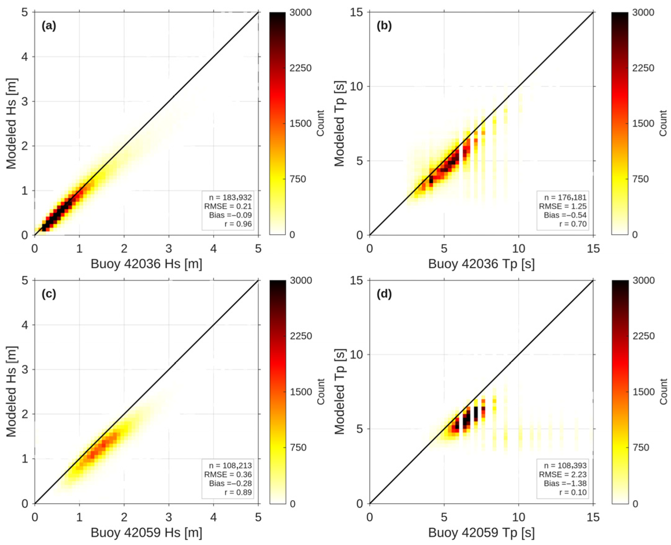
Figure A1, Figure A2, Figure A3, Figure A4, Figure A5 and Figure A6 present the validation results for the remaining eight NDBC buoys (42020, 42035, 42002, 42040, 42056, 42057, 42036, and 42059) not shown in the main text. Figure A1, Figure A2 and Figure A3 display the 2017 time series of Hs and Tp for each buoy, comparing WW3 model output against buoy observations. Figure A4, Figure A5 and Figure A6 presents the corresponding scatter plots for the same buoys. These results are consistent with the validation metrics reported in Table 2 and support the conclusions drawn from three representative buoys (42001, 42058, and 42055) presented in the main text.
Figure A1.
Hourly time series comparison of simulated (WW3 model) and observed wave parameters for the year 2017 at buoys 42020, 42035, and 42002: (a) Hs at buoy 42020, (b) Tp at buoy 42020, (c) Hs at buoy 42035, (d) Tp at buoy 42035, (e) Hs at buoy 42002, and (f) Tp at buoy 42002.
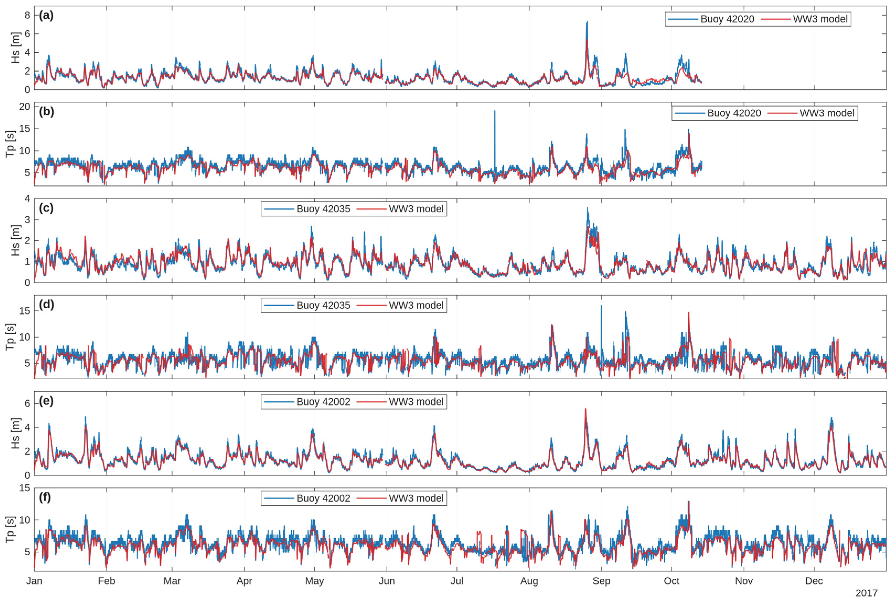
Figure A2.
Hourly time series comparison of simulated (WW3 model) and observed wave parameters for the year 2017 at buoys 42040, 42056, and 42057: (a) Hs at buoy 42040, (b) Tp at buoy 42040, (c) Hs at buoy 42056, (d) Tp at buoy 42056, (e) Hs at buoy 42057, and (f) Tp at buoy 42057.
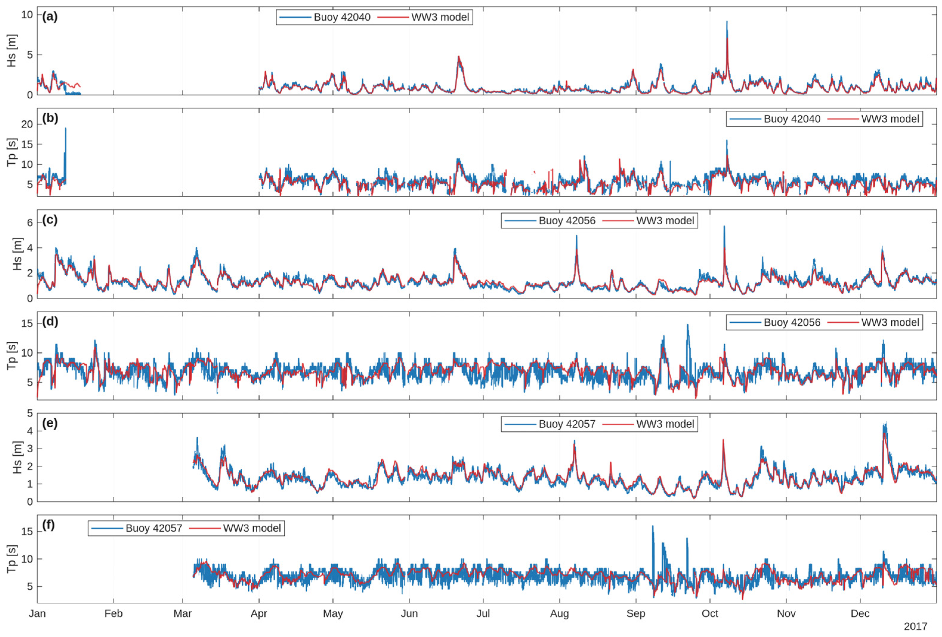
Figure A3.
Hourly time series comparison of simulated (WW3 model) and observed wave parameters for the year 2017 at buoys 42036, and 42059: (a) Hs at buoy 42036, (b) Tp at buoy 42036, (c) Hs at buoy 42059, (d) Tp at buoy 42059.
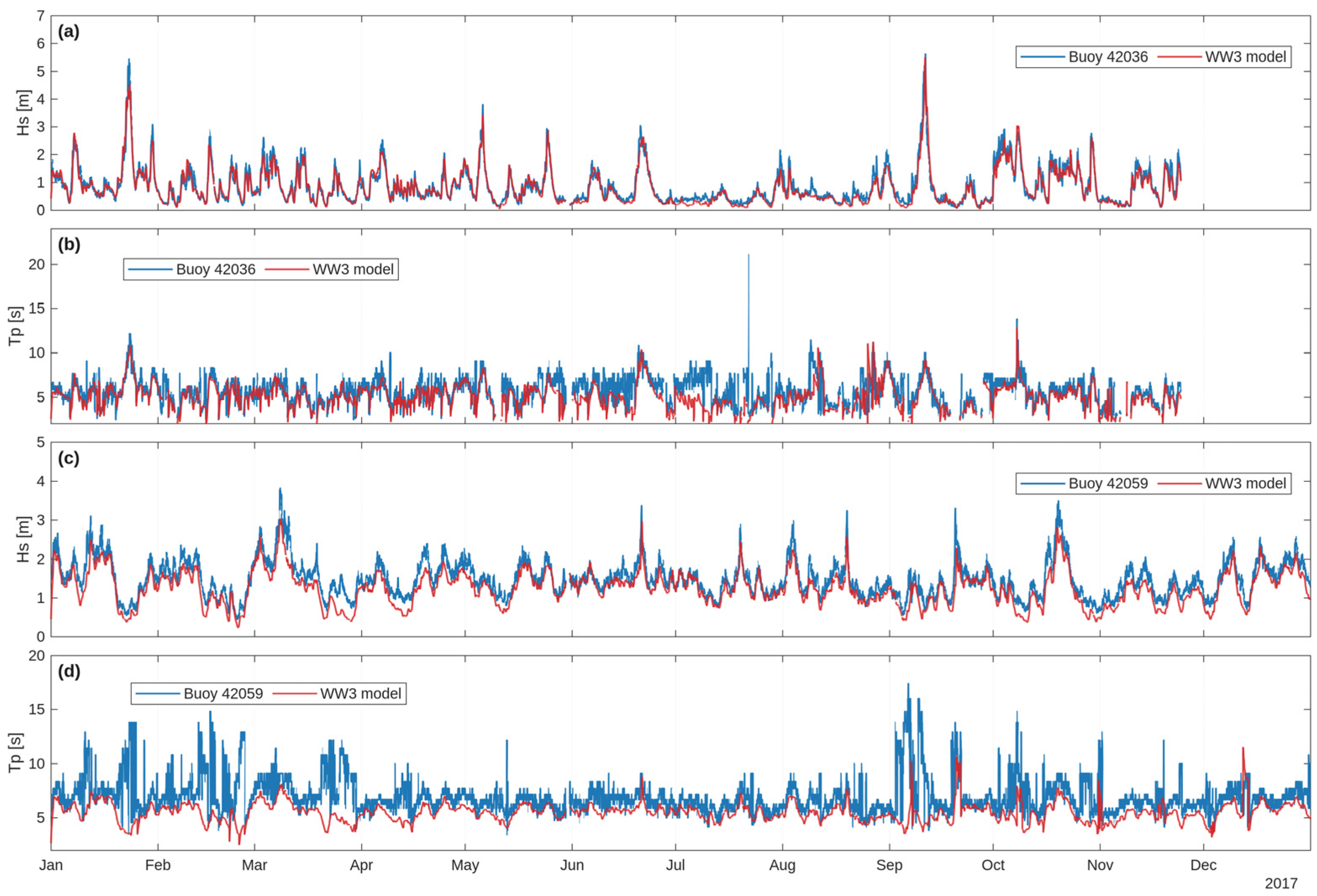
Figure A4.
Density scatter plots comparing hourly observed (x-axis) and modeled (y-axis) Hs and Tp. Panels (a,b) correspond to buoy 42020, panels (c,d) correspond to buoy 42035, while panels (e,f) correspond to buoy 42002. Color scale indicates the number of data points (count) per bin. The red dashed line indicates the 1:1 agreement line between observations and model results.
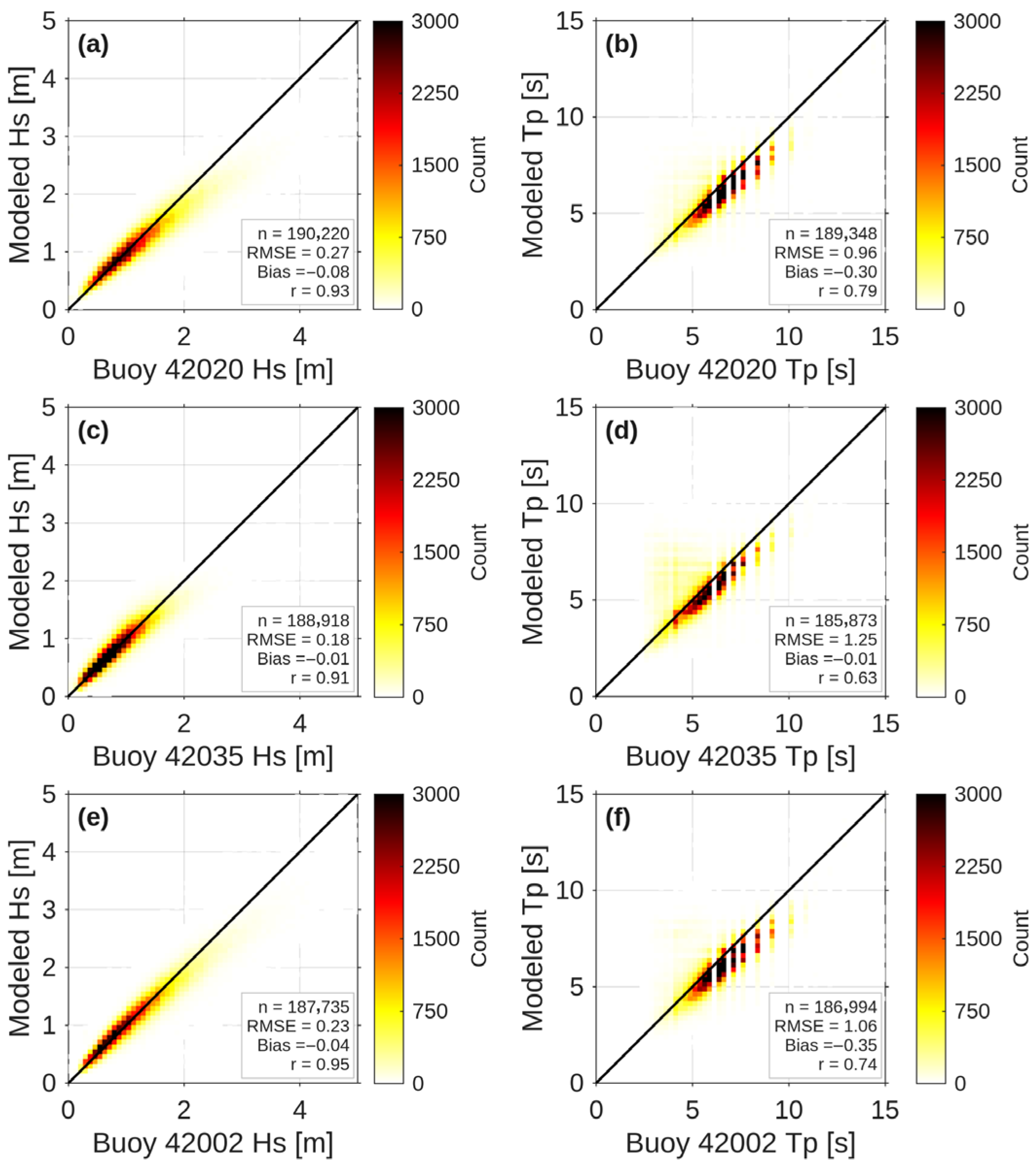
Figure A5.
Density scatter plots comparing hourly observed (x-axis) and modeled (y-axis) Hs and Tp. Panels (a,b) correspond to buoy 42040, panels (c,d) correspond to buoy 42056, while panels (e,f) correspond to buoy 42057. Color scale indicates the number of data points (count) per bin. The red dashed line indicates the 1:1 agreement line between observations and model results.
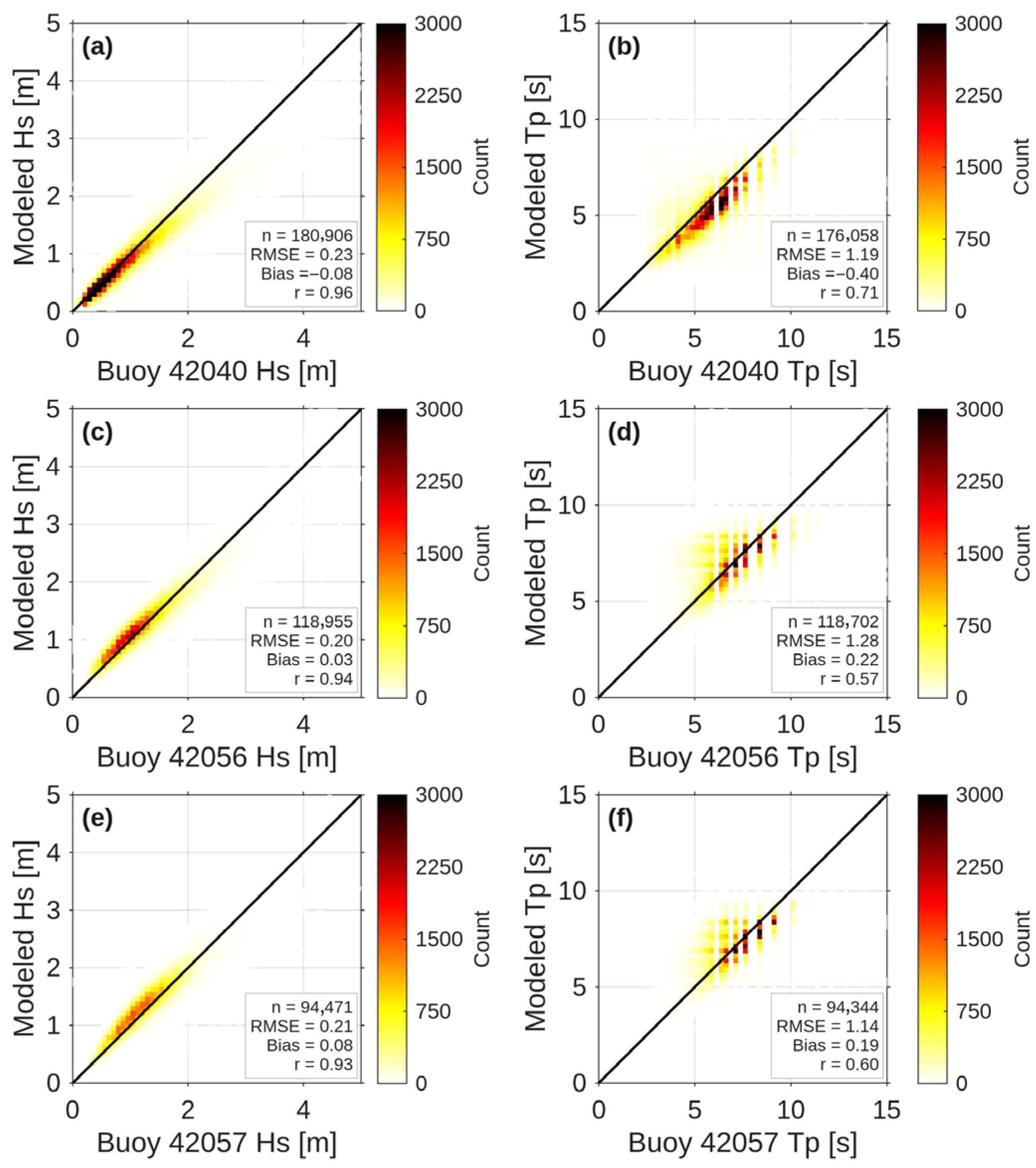
Figure A6.
Density scatter plots comparing hourly observed (x-axis) and modeled (y-axis) Hs and Tp. Panels (a,b) correspond to buoy 42036, panels (c,d) correspond to buoy 42059. Color scale indicates the number of data points (count) per bin. The red dashed line indicates the 1:1 agreement line between observations and model results.
References
- Shepard, A.N.; Valentine, J.F.; D’Elia, C.F.; Yoskowitz, D.W.; Dismukes, D.E. Economic Impact of Gulf of Mexico Ecosystem Goods and Services and Integration Into Restoration Decision-Making. Goms 2013, 31, 2. [Google Scholar] [CrossRef] [Scilit]
- Didenkulova, E.; Didenkulova, I.; Medvedev, I. Freak Wave Events in 2005–2021: Statistics and Analysis of Favourable Wave and Wind Conditions. Nat. Hazards Earth Syst. Sci. 2023, 23, 1653–1663. [Google Scholar] [CrossRef] [Scilit]
- Azevedo, L.; Marcon, G.; Meyers, S.; Luther, M. Rogue Wave Indicators from Global Models and Buoy Data. Ocean Sci. 2026, 22, 367–386. [Google Scholar] [CrossRef] [Scilit]
- Beven, J.L.; Stewart, S.R.; Lawrence, M.B.; Avila, L.A.; Franklin, J.L.; Pasch, R.J. ANNUAL SUMMARY: Atlantic Hurricane Season of 2001. Mon. Weather Rev. 2003, 131, 1454–1484. [Google Scholar] [CrossRef] [Scilit]
- Needham, H.F.; Keim, B.D. A Storm Surge Database for the US Gulf Coast. Intl J. Climatol. 2012, 32, 2108–2123. [Google Scholar] [CrossRef] [Scilit]
- Kirezci, E.; Young, I.R.; Ranasinghe, R.; Muis, S.; Nicholls, R.J.; Lincke, D.; Hinkel, J. Projections of Global-Scale Extreme Sea Levels and Resulting Episodic Coastal Flooding over the 21st Century. Sci. Rep. 2020, 10, 11629. [Google Scholar] [CrossRef] [Scilit] [PubMed]
- IPCC. Sea Level Change. In Climate Change 2013—The Physical Science Basis; Church, J.A., Clark, P.U., Eds.; Cambridge University Press: Cambridge, UK, 2013; pp. 1137–1216. [Google Scholar] [CrossRef] [Scilit]
- Reguero, B.G.; Losada, I.J.; Méndez, F.J. A Recent Increase in Global Wave Power as a Consequence of Oceanic Warming. Nat. Commun. 2019, 10, 205. [Google Scholar] [CrossRef] [Scilit] [PubMed]
- Young, I.R.; Zieger, S.; Babanin, A.V. Global Trends in Wind Speed and Wave Height. Science 2011, 332, 451–455. [Google Scholar] [CrossRef] [Scilit]
- Morim, J.; Hemer, M.; Wang, X.L.; Cartwright, N.; Trenham, C.; Semedo, A.; Young, I.; Bricheno, L.; Camus, P.; Casas-Prat, M.; et al. Robustness and Uncertainties in Global Multivariate Wind-Wave Climate Projections. Nat. Clim. Change 2019, 9, 711–718. [Google Scholar] [CrossRef] [Scilit]
- Odériz, I.; Losada, I.J.; Silva, R.; Mori, N. On the Need to Integrate Interannual Natural Variability into Coastal Multihazard Assessments. Sci. Rep. 2024, 14, 16998. [Google Scholar] [CrossRef] [Scilit] [PubMed]
- Semedo, A.; Sušelj, K.; Rutgersson, A.; Sterl, A. A Global View on the Wind Sea and Swell Climate and Variability from ERA-40. J. Clim. 2011, 24, 1461–1479. [Google Scholar] [CrossRef] [Scilit]
- Appendini, C.M.; Torres-Freyermuth, A.; Salles, P.; López-González, J.; Mendoza, E.T. Wave Climate and Trends for the Gulf of Mexico: A 30-Yr Wave Hindcast. J. Clim. 2014, 27, 1619–1632. [Google Scholar] [CrossRef] [Scilit]
- Kumar, P.; Yadav, A.; Sardana, D.; Prasad, R. Rajni Extreme Wave Height Response to Climate Modes and Its Association with Tropical Cyclones over the Indo-Pacific Ocean. Ocean Eng. 2024, 296, 116789. [Google Scholar] [CrossRef] [Scilit]
- Panchang, V.; Kwon Jeong, C.; Demirbilek, Z. Analyses of Extreme Wave Heights in the Gulf of Mexico for Offshore Engineering Applications. J. Offshore Mech. Arct. Eng. 2013, 135, 031104. [Google Scholar] [CrossRef] [Scilit]
- Montoya, R.D.; Menendez, M.; Osorio, A.F. Exploring Changes in Caribbean Hurricane-Induced Wave Heights. Ocean Eng. 2018, 163, 126–135. [Google Scholar] [CrossRef] [Scilit]
- WAVEWATCH III Development Group. User Manual and System Documentation of WAVEWATCH III® Version 6.07; NOAA/NWS/NCEP/MMAB: College Park, MD, USA, 2019; p. 465.
- National Data Buoy Center (NDBC). NDBC Buoy Data: Stations 42001, 42002, 42020, 42035, 42036, 42040, 42055, 42056, 42058 and 42059 (1998–2022); National Oceanic and Atmospheric Administration (NOAA): Silver Spring, MD, USA, 2021.
- Kendall, M.G. Rank Correlation Methods; Charles Griffin & Co.: London, UK, 1948. [Google Scholar]
- Sen, P.K. Estimates of the Regression Coefficient Based on Kendall’s Tau. J. Am. Stat. Assoc. 1968, 63, 1379–1389. [Google Scholar] [CrossRef]
- Partal, T.; Kahya, E. Trend Analysis in Turkish Precipitation Data. Hydrol. Process. 2006, 20, 2011–2026. [Google Scholar] [CrossRef] [Scilit]
- Copernicus Climate Change Service (C3S). ERA5: Fifth Generation of ECMWF Atmospheric Reanalysis of the Global Climate; Copernicus Climate Change Service: Reading, UK, 2017. [Google Scholar]
- GEBCO Compilation Group. GEBCO 2021 Grid—A Continuous Terrain Model of the Global Oceans and Land; BODC, British Oceanographic Data Centre: Liverpool, UK, 2021. [Google Scholar]
- Wessel, P.; Smith, W.H.F. A Global, Self-consistent, Hierarchical, High-resolution Shoreline Database. J. Geophys. Res. 1996, 101, 8741–8743. [Google Scholar] [CrossRef] [Scilit]
- Ardhuin, F.; Rogers, E.; Babanin, A.V.; Filipot, J.-F.; Magne, R.; Roland, A.; Van Der Westhuysen, A.; Queffeulou, P.; Lefevre, J.-M.; Aouf, L.; et al. Semiempirical Dissipation Source Functions for Ocean Waves. Part I: Definition, Calibration, and Validation. J. Phys. Oceanogr. 2010, 40, 1917–1941. [Google Scholar] [CrossRef] [Scilit]
- Guillou, N. Estimating Wave Energy Flux from Significant Wave Height and Peak Period. Renew. Energy 2020, 155, 1383–1393. [Google Scholar] [CrossRef] [Scilit]
- von Storch, H.; Navarra, A. Analysis of Climate Variability: Applications of Statistical Techniques; Springer: Berlin/Heidelberg, Germany, 1995. [Google Scholar]
- Kendall, M.G.; Stuart, A. The Advanced Theory of Statistics; Charles Griffin & Co. Ltd.: London, UK, 1968; Volume 3. [Google Scholar]
- Salas, J.D.; Delleur, J.W.; Yevjevich, V.; Lane, W.L. Applied Modeling of Hydrologic Time Series; Water Resources Publications: Littleton, CO, USA, 1980. [Google Scholar]
- NOAA Climate Prediction Center. Oceanic Niño Index (ONI) 2020; NOAA: Silver Spring, MD, USA, 2020.
- Enfield, D.B.; Mestas-Nuñez, A.M.; Trimble, P.J. The Atlantic Multidecadal Oscillation and Its Relation to Rainfall and River Flows in the Continental U.S. Geophys. Res. Lett. 2001, 28, 2077–2080. [Google Scholar] [CrossRef] [Scilit]
- Hurrell, J.W. Decadal Trends in the North Atlantic Oscillation: Regional Temperatures and Precipitation. Science 1995, 269, 676–679. [Google Scholar] [CrossRef] [Scilit]
- Sørensen, O.R.; Kofoed-Hansen, H.; Rugbjerg, M.; Sørensen, L.S. A Third-Generation Spectral Wave Model Using an Unstructured Finite Volume Technique. In Proceedings of the Coastal Engineering 2004; World Scientific Publishing Company: Lisbon, Portugal, 2005; pp. 894–906. [Google Scholar]
- Ahn, S.; Neary, V.S. Non-Stationary Historical Trends in Wave Energy Climate for Coastal Waters of the United States. Ocean Eng. 2020, 216, 108044. [Google Scholar] [CrossRef] [Scilit]
- Cao, Y.; Dong, C.; Young, I.R.; Yang, J. Global Wave Height Slowdown Trend during a Recent Global Warming Slowdown. Remote Sens. 2021, 13, 4096. [Google Scholar] [CrossRef] [Scilit]
- Jing, R.; Chen, C.; Hu, S.; Sasa, K.; Yu, H.; Hu, Y. Spatial-Temporal Shipping Risk Assessment along Asia-Europe Route Due to Ocean Waves. Ocean Coast. Manag. 2025, 270, 107922. [Google Scholar] [CrossRef] [Scilit]
- Gommosani, M.E.; Alghaffari, S.; Ghonaim, S.; Hassan, R.; Tonbol, K. Extreme Weather Events in Jeddah (2000–2024) and Their Implications for Maritime Port Operations under Global Climate Risk Frameworks. Theor. Appl. Clim. 2026, 157, 53. [Google Scholar] [CrossRef] [Scilit]
- Spaulding, M.L. State of the Art Review and Future Directions in Oil Spill Modeling. Mar. Pollut. Bull. 2017, 115, 7–19. [Google Scholar] [CrossRef] [Scilit]
- Falnes, J. A Review of Wave-Energy Extraction. Mar. Struct. 2007, 20, 185–201. [Google Scholar] [CrossRef] [Scilit]
- Reguero, B.G.; Losada, I.J.; Méndez, F.J. A Global Wave Power Resource and Its Seasonal, Interannual and Long-Term Variability. Appl. Energy 2015, 148, 366–380. [Google Scholar] [CrossRef] [Scilit]
- Walker, N.D.; Leben, R.R.; Balasubramanian, S. Hurricane-forced Upwelling and Chlorophyll a Enhancement within Cold-core Cyclones in the Gulf of Mexico. Geophys. Res. Lett. 2005, 32, 2005GL023716. [Google Scholar] [CrossRef] [Scilit]
- Wang, C.; Enfield, D.B. The Tropical Western Hemisphere Warm Pool. Geophys. Res. Lett. 2001, 28, 1635–1638. [Google Scholar] [CrossRef] [Scilit]
- Dodet, G.; Bertin, X.; Taborda, R. Wave Climate Variability in the North-East Atlantic Ocean over the Last Six Decades. Ocean Model. 2010, 31, 120–131. [Google Scholar] [CrossRef] [Scilit]
- Maia, N.Z.; Almeida, L.P.; Nicolodi, J.L.; Calliari, L.; Castelle, B. Long-Term Trends and Wave Climate Variability in the South Atlantic Ocean: The Influence of Climate Indices. Reg. Stud. Mar. Sci. 2023, 66, 103131. [Google Scholar] [CrossRef] [Scilit]
- Caires, S.; Sterl, A. 100-Year Return Value Estimates for Ocean Wind Speed and Significant Wave Height from the ERA-40 Data. J. Clim. 2005, 18, 1032–1048. [Google Scholar] [CrossRef] [Scilit]
- Knight, J.R.; Folland, C.K.; Scaife, A.A. Climate Impacts of the Atlantic Multidecadal Oscillation. Geophys. Res. Lett. 2006, 33, 2006GL026242. [Google Scholar] [CrossRef] [Scilit]
- Cai, W.; Santoso, A.; Collins, M.; Dewitte, B.; Karamperidou, C.; Kug, J.-S.; Lengaigne, M.; McPhaden, M.J.; Stuecker, M.F.; Taschetto, A.S.; et al. Changing El Niño–Southern Oscillation in a Warming Climate. Nat. Rev. Earth Environ. 2021, 2, 628–644. [Google Scholar] [CrossRef] [Scilit]
- Bromirski, P.D.; Cayan, D.R.; Helly, J.; Wittmann, P. Wave Power Variability and Trends across the North Pacific. JGR Oceans 2013, 118, 6329–6348. [Google Scholar] [CrossRef] [Scilit]
- Wang, X.L.; Wan, H.; Zwiers, F.W.; Swail, V.R.; Compo, G.P.; Allan, R.J.; Vose, R.S.; Jourdain, S.; Yin, X. Trends and Low-Frequency Variability of Storminess over Western Europe, 1878–2007. Clim. Dyn. 2011, 37, 2355–2371. [Google Scholar] [CrossRef] [Scilit]
- Young, I.R.; Ribal, A. Multiplatform Evaluation of Global Trends in Wind Speed and Wave Height. Science 2019, 364, 548–552. [Google Scholar] [CrossRef] [Scilit]
- Izaguirre, C.; Méndez, F.J.; Menéndez, M.; Losada, I.J. Global Extreme Wave Height Variability Based on Satellite Data: Worldwide Extreme Wave Height. Geophys. Res. Lett. 2011, 38. [Google Scholar] [CrossRef] [Scilit]

Disclaimer/Publisher’s Note: The statements, opinions and data contained in all publications are solely those of the individual author(s) and contributor(s) and not of MDPI and/or the editor(s). MDPI and/or the editor(s) disclaim responsibility for any injury to people or property resulting from any ideas, methods, instructions or products referred to in the content. |
© 2026 by the authors. Licensee MDPI, Basel, Switzerland. This article is an open access article distributed under the terms and conditions of the Creative Commons Attribution (CC BY) license.