


Abstract
The water–land classification is fundamental for shoreline extraction and coastal habitat mapping, which is the basis of a comprehensive assessment and ecosystem-based coastal zone management. This study aims to separate water and land for coastal zones by taking advantage of both high-resolution satellite imagery and airborne lidar point clouds. Considering physical principles of optical remote sensing and lidar, we developed a prior knowledge-based localization classification approach that eliminates the need for collecting training sets and handling temporal differences across multiple data sources. Our approach first created the initial classification using the WorldView-2 (WV2) Normalized Difference Water Index. Then, the Connected Components Labeling algorithm was used to create a non-overlapping partition of the working area. The third step involved processing the water blocks using prior land cover knowledge. Finally, we used lidar point clouds to refine the initial water blocks and their neighboring areas. This classification approach showed promising results along Matagorda Bay, Texas, an approximately 2449 km2 area that is covered by 26 WV2 images and 1568 lidar tiles.
1. Introduction
Coastal areas are facing complex challenges due to multiple environmental stressors including relative sea-level rise due to global climate change, overfishing, wastewater pollution, coastal development, and eutrophication. To address these complexities, the National Oceanic and Atmospheric Administration (NOAA) Integrated Ecosystem Assessment approach [1] was widely adopted by coastal communities. Detailed coastal habitat maps are the basis of an integrated ecosystem assessment and an ecosystem-based coastal zone management approach [2,3,4,5], which would allow assessments and visualization of biological and physical characteristics of the estuary on a seasonal and temporal basis. The water–land classification is fundamental for coastal habitat mapping. Water identification is not a trivial topic for the coastal zone [6,7,8,9,10]. By presenting detailed mathematical formulations, the relevant algorithms, and comprehensive discussions, this paper extends our previous IGARSS 2023 publication [6]. The earlier article mainly included conceptual descriptions of the proposed methods, with results limited to classification map and accuracy. In contrast, the current paper offers a more thorough and rigorous presentation of methodologies and experimental analyses.
1.1. Water Classification by Lidar and Satellite Imagery
Remote sensing techniques have been an important tool for mapping and monitoring coastal habitats over the last decades [11,12,13,14]. In general, the water classification is implemented on informative features derived from imagery and/or lidar point clouds by various classification algorithms. Moreover, the investigators may assume different characteristics of water for their study areas. The simplest strategy is directly to delimit water areas by a given water surface elevation line on a digital surface model generated from all points of a lidar point cloud [15]. Such an approach typically assumes that surface water is flat as gravity always pulls liquid molecules down [16]. This assumption is robust for inland water bodies. However, in coastal areas, total water-level elevation fluctuates due to tides, surge, and wave-induced runup [17]. Additionally, water surface has different elevations at different locations in coastal bays at the same time due to their seabed topography [18]. Furthermore, water bodies may stand on isolated ponds at low tide that have different surface elevations, though these waters may connect to open water at high tide [19].
Water classification from lidar point clouds could use point 3D coordinates and/or intensity. The approach of using only 3D coordinates is based on the detection of vertical height changes [20,21]. This approach assumes that planimetric lidar point distribution should be sufficiently consistent and water areas are in high-relief environments. Such an assumption is not always correct for low-relief topography, such as coastal deltas [19]. When point intensity is used the intensity feature should be normalized by the calibration routines [22,23]. Water is typically characterized by a very large range of intensity signatures and a lower point density. The variability in the intensity signature leads to portions of water bodies being misclassified as similar land cover classes [24]. Recently, airborne multispectral lidar sensors have become capable of acquiring intensity values from targets at multiple wavelengths. Shaker et al. [25] takes advantage of the potential for active spectral indices for land–water classification in near-shore and river environments.
Optical satellite imagery and airborne lidar are widely used for surface water detection, either independently or in combination [26]. Lee et al. [27] used the RGB channels of orthoimages at the corresponding (X, Y) coordinates to directly obtain spectral information from lidar points for water classification. The approach can obtain better spectral information of land cover features for lidar points, but it requires matching both acquisition time and spatial resolution of both lidar and optical data. Recent work shows that high-resolution imagery, combined with advanced classifiers and water indices, can significantly improve the extraction of water bodies with large training datasets [13,14,28]. The Normalized Difference Water Index (NDWI) is commonly used for spectral indices for water recognition from surrounding land features [28]. The commonly used water classifiers typically include support vector machines, decision tree and deep learning [29,30,31].
Prior knowledge data has been employed for lidar water classification. For instance, the existing historical coastline was used as a basis for designing a training set [26]. In this study, we use prior knowledge of land cover, high-resolution satellite imagery and airborne lidar point clouds to create a water–land classification for a bay area along the Gulf of Mexico.
1.2. Basic Settings and Overall Strategy
Our working region was the low-lying coastal zone around Matagorda Bay, Texas, which had no significant elevation changes perpendicular to the shorelines. Further, the water surface did not remain flat over the whole coastal bay, and water bodies in the area had different surface elevations. We utilized the Coastal Change Analysis Program (C-CAP) data [32], a 30 m spatial resolution land cover product, for prior knowledge of the large permanent waters (gulf and bay). This was reasonable because the large permanent waters in the Texas coastal zone had no significant change due to the relatively short interval of data products and the extensive environmental conservation practices in the bay.
We developed a novel classification approach to take advantage of high-resolution satellite imagery, airborne lidar point clouds, and prior knowledge. The overall strategy consisted of two components: (1) a localization classifier to reduce mislabeling from imagery and point clouds classification and (2) a progressive approach of using prior knowledge to reduce efforts of generating the training set. Water mislabeling could occur in both spectral images and point clouds in coastal zones. For example, a spectral classifier may label spilling and plunging breakers as land due to the white foam of the breaking waves which differs from the typical spectral response of water. Mislabeling could also occur in very shallow water or turbid water. A point cloud classifier may classify these waves as low vegetation due to elevation changes in the waves. These two types of mislabeling have different neighboring components due to different physical reasons. Our localization classifier effectively corrected the mislabelings by considering the neighboring attributes. On the other hand, it is time- and labor-intensive to generate training sets for supervised classifications. Currently available land cover datasets allow us to develop a progressive approach that eliminates the need for manually generating training sets and handling temporal differences in multiple data sources.
The classification generated a binary thematic map distinguishing between land and water. This map can serve as a basis for subsequent classifications, such as identifying bare soil or grasses on land, or submerged vegetation in water.
2. Study Area and Data Sets
The Matagorda Bay region, Texas, is one of seven major estuaries along the Gulf Coast of Texas. The bay is separated from the Gulf of Mexico by Matagorda Peninsula, which has around 45 km of uninhabited coastline and numerous storm washover channels, so the shoreline has changed over time. This region provides a habitat for a wide variety of wildlife. Matagorda Bay typically experiences a small tidal range, often classified as microtidal, with daily fluctuations generally around 0.3 to 0.6 m according to NOAA tide tables. Water level is not the same throughout the bay since tidal lags, friction in narrow inlets, wind, and river runoff create significant spatial variations. Additionally, small water-level fluctuations could lead to large changes in inundation area due to its gentle low-lying tidal flats.
The data used consisted of 26 WorldView-2 (WV2) images acquired on 17 November 2012, 5 May 2013, and 16 December 2013, as well as 1568 lidar 1500 m × 1500 m tiles acquired by the South Texas FEMA (Federal Emergency Management Agency) lidar project with acquisition dates from 4 January 2018 to 23 February 2018 and 24 January 2019 to 29 January 2019. The lidar data utilizes the NAD83 (2011) horizontal datum, projected in UTM Zone 14, and is referenced vertically to the NAVD88 datum. Each lidar point was labeled by the lidar surveyors into four categories: processed but unclassified, ground, water, and noise.
The FEMA lidar project’s original specifications included an average point density of 2.5 points per square meter, a flight altitude (AGL) between 1700 and 2294 m, a field of view ranging from 34° to 59°, and a minimum side overlap of 12%. Five different sensors were utilized for data collection: Leica ALS70 and Leica ALS80 manufactured by Leica Geosystems AG, Heerbrugg, Switzerland, Riegl VQ-1560i and Riegl LMS-Q1560 manufactured by RIEGL LMS GmbH, Horn, Austria, and Optech/Teledyne ALTM Orion H300 manufactured by Teledyne Optech, Vaughan, ON, Canada. All airborne lidar sensors operated at a wavelength of 1064 nm, with a beam divergence ranging from 0.15 to 0.26 milliradians (measured at the 1/e2 or 1/e level). Each sensor was capable of recording multiple returns per outgoing laser pulse. The intensity of the returns is also captured during aerial acquisition. Across the study area, the proportion of points with single returns varied by tile, ranging from 79% to 99%. The lidar sensors can provide both (x, y, z) coordinates and the intensity of a point. Lidar intensity measures the strength of a laser pulse’s return, reflecting how much energy is received back by the sensor from a surface. Because intensity values are typically relative rather than calibrated, they can vary depending on flight conditions, scanner type, or environmental factors. As a result, intensity is generally more useful for qualitative visual interpretation than for precise quantitative analysis. In this study, we utilize only the (x, y) position and elevation (z) of lidar points.
The WV2 imagery used by the study consisted of eight-band multispectral imagery with 2 m spatial resolution, including coastal (400 nm to 450 nm), blue (450 nm to 510 nm), green (510 nm to 580 nm), yellow (585 nm to 625 nm), red (630 nm to 690 nm), red edge (705 nm to 745 nm), and Near-Infrared-1 (NIR1, 770 nm to 895 nm) and Near-Infrared-2 (NIR2, 860 nm to 1040 nm) bands. These images were obtained by our project “Enhanced 3-D Mapping for Habitat, Biodiversity, and Flood Hazard Assessments of Coastal and Wetland Areas of the Southern US” funded by the U.S. National Science Foundation (Award Number 1762493). For our study area, available WV2 images were visually inspected, and only cloud-free scenes were selected for analysis.
The Coastal Change Analysis Program (C-CAP) [32], administered by the National Oceanic and Atmospheric Administration (NOAA), provides land cover data at a spatial resolution of 30 m for the coastal areas of the contiguous United States. C-CAP data are updated every five years from multiple dates of remotely sensed Landsat imagery and ancillary information. Most regions now have land cover records spanning more than 20 years. The C-CAP program provides reliable, repeatable, and consistent land cover data for U.S. coastal areas, supporting science, management, and policy efforts related to coastal environments. We use the 2016 C-CAP regional land cover dataset as prior knowledge.
3. Methods
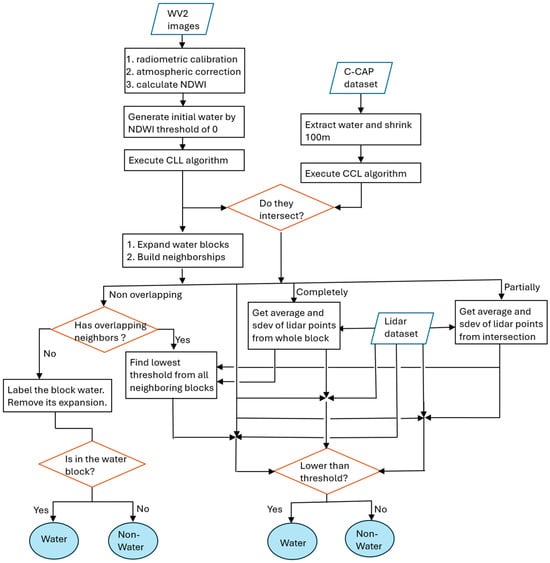
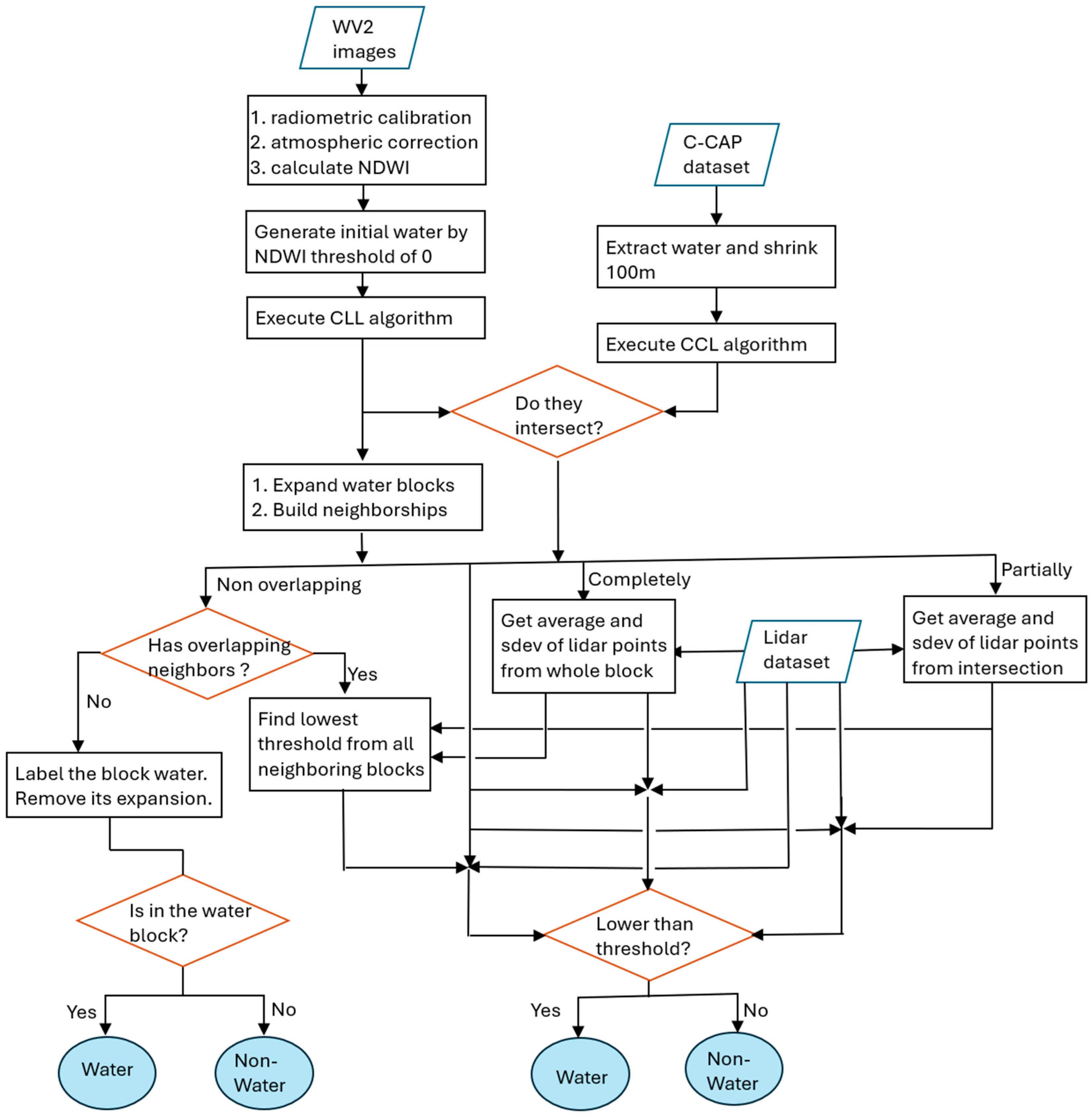
Our classification approach consists of four components: (1) WV2 initial water classification, (2) C-CAP water cover, (3) data localization, and (4) refinement using lidar data. Figure 1 shows flowchart of the classification approach.
Figure 1.
Flowchart of the water classification.
3.1. WV2 Initial Water Classification
First, radiometric calibration, atmospheric correction and georectification were performed on the 26 WV2 images using MATLAB R2018b and Python 3.7 codes provided by the Polar Geospatial Center at the University of Minnesota. The atmospheric correction included Rayleigh scattering correction, however aerosol correction was not applied. The Normalized Difference Water Index (NDWI) uses visible green and near-infrared reflectance according to the following equation [33]:
where and denote surface reflectance of the green and NIR2 bands of WV2, respectively. NDWI was subsequently used to distinguish water from land for an initial water classification:
where denotes the NDWI value at pixel location and represents the corresponding binary classification result (1 = water, 0 = non-water). This initial water classification identified both large water bodies (gulf and bay) and numerous small, isolated water bodies (ponds and water surfaces between the breakers).
After classification of individual WV2 images, the resulting classification images were merged into mosaic files. When overlaps occurred, priority was based on an acquisition date, with more recent imagery given precedence (16 December 2013 > 5 May 2013 > 17 November 2012).
3.2. C-CAP Water Cover
In addition to creating a WV2 water classification, we extracted water bodies from the 2016 C-CAP regional land cover dataset [33]. To delineate reliable open-water areas (gulfs and bays) from C-CAP data, we shrunk the original C-CAP water extent by 100 m using a binary dilation operation from mathematical morphology. As a result, the derived gulf and bay water regions are intentionally more conservative and generally smaller than the true water extent.
Shrinking water areas is conceptually equivalent to expanding non-water regions. Practically, this shrinking is implemented by first resampling the 30 m pixel into 10 m pixel, followed by 10 iterations of binary dilations using a 3 × 3 structuring element (kernel) to expand non-water class. The binary dilation is defined mathematically as follows [34]:
where A represents the C-CAP non-water raster, B is the 3 × 3 kernel, is the reflection of B overlapping with foreground pixels. We can express Equation (3) as a function: for an input C-CAP non-water raster A and output expanded C-CAP non-water raster B, for any (where 1 indicates water, 0 for non-water),
where and represent the pixel values at position in A and B, respectively. Indices and define the spatial footprint of the 3 × 3 kernel. Equation (3) implies that, for each water pixel, if its 3 × 3 kernel covers any non-water pixel, the center pixel is set to non-water.
3.3. Data Localization
3.3.1. Obtaining Water Blocks
To identify water regions, the Connected Components Labeling (CCL) algorithm [35] was independently applied to the WV2-derived water classification and the extracted C-CAP water cover. The CCL algorithm scans an image and groups adjacent pixels into connected components based on pixel connectivity. In this study, eight-connectivity was used. For a pixel at coordinates , the eight-connected neighborhood consists of all pixels whose coordinates differ by at most one in either direction (including diagonals). Through this process, spatially contiguous pixels with identical values are grouped into connected components, referred to here as water blocks. Each connected component is then assigned a unique label, which is applied to all pixels belonging to that component.
Using CCL, two types of water regions were recognized: (1) initial water blocks from the WV2 water classification and (2) water blocks from extraction C-CAP water. Both WV2 and C-CAP water blocks were limited to 750 × 750 pixels (corresponding to 1500 m × 1500 m). The labeled image resulting from WV2 water classification is denoted as Label_wv2, while the labeled image resulting from C-CAP is referred to as Label_ccap. For each labeled region of Label_wv2, the total number of pixels—representing the area of the water block—was counted and stored in a separate image referred to as Area_wv2. Specifically, at each corresponding position, Label_wv2 contains the label of a water block, while Area_wv2 records the area associated with that block. The Connected Components Labeling algorithm is a standard routine in image processing. Its details are well-established and are therefore not repeated here.
3.3.2. Expanding WV2 Water Blocks and Constructing Their Neighborship
The initial WV2 water blocks did not capture all possible water features due to the spectral variance, notably missing some shallow, turbid, aquatic plants or surf-zone water areas. To address this limitation, we expanded the WV2 water blocks. Expansion halted when two growing water blocks intersected or when the expansion reached 30 pixels (60 m). The process created a non-overlapping partition of the study area based on the WV2 initial water classification. C-CAP water blocks were not expanded.
The expansion algorithm applies a 3 × 3 kernel operation over the entire image up to 30 times, which is defined in the following. For brevity, we denote the following:
: the input WV2 labeled raster (Label_wv2);
: the corresponding water block area raster (Area_wv2);
: the output raster after expansion.
At a single 3 × 3 kernel operation, the algorithm operates as follows:
If , set .
For any ,
where and is the pixel value at row and column in raster . and are the pixel values at position in the input raster and output raster , respectively.
The function returns the coordinates with the maximum value in raster within the 3 × 3 neighborhood, so is the coordinates of the maximum value. If no neighboring water pixels exist ( for all neighbors), , so , meaning no expansion occurs. The algorithm naturally gives priority to larger blocks. After 30 iterations, the output raster becomes the expansion of Label_wv2, referred to as Labelexp_wv2.
Continuous water bodies in rivers and streams may be segmented into distinct water blocks during NDWI thresholding due to spectral variation. These separated water bodies may be reconnected through the morphological expansion. The resulting connected water regions help maintain the integrity of river or stream networks in the classified image.
The next step is to construct neighboring relationships for each water region in Labelexp_wv2. We use a jagged arrays in C# (, equivalent to a nested list in Python) to store the neighbor set for each region. The water label serves as row index for the array.
The neighbor identification is defined mathematically as follows. For brevity, we denote raster as Labelexp_wv2. For any ,
where is the water label at position . contains distinct neighboring water labels different to within the 3 × 3 neighborhood at centered at . Then existing is then updated by adding the elements of .
3.3.3. Assessing Statuses of WV2 Water Overlaps over CCAP Water
We analyzed spatial intersections between the WV2 water blocks (Label_wv2) and C-CAP water blocks (Label_ccap). Intersections were categorized into three types: (1) complete overlap, (2) partial overlap, and (3) no overlap between water bodies. The WV2 water blocks that completely overlap C-CAP water are typically found within gulfs or bays, representing high confidence water bodies. The WV2 water blocks with no overlap often correspond to isolated small ponds located away from open waters, thus exhibiting low confidence. Blocks exhibiting partial overlap with the C-CAP water generally correspond to potential near-shore areas. The intersection algorithm is expressed in output raster Label_intersect as
where , , and represent the pixel values at position at .
To facilitate further analysis, we constructed an array to indicate the presence of each water label within the raster Label_intersect. Each water label serves as the row index of the array. As the implementation is straightforward, additional algorithmic details are omitted here for brevity.
3.4. Refinement Using Lidar Data
3.4.1. Generating Surface Elevation and Computing Statistics
We generated a digital surface model (DSM) using a three-nearest neighbor inverse distance weighting (IDW) interpolation algorithm, which estimates values at unmeasured locations by averaging known sample points, giving closer points higher weights based on the inverse square of their distance. For a target pixel center at with unknown elevation , and its three-nearest neighbors at , , and with known elevations , , and , the interpolated elevation is given by
where represents the squared Euclidean distance between the target pixel and each neighbor. The three-nearest points are identified from the lidar point clouds within a 2 m × 2 m search window centered at . Pixels with no lidar points within this search window were assigned as no-data.
We then calculated summary statistics on the DSM for each water intersection defined by Label_intersect as follows:
where WI denotes a water intersection on Label_intersect defined by Equation (10) and n is the number of DSM pixels within WI excluding no-data pixels.
To determine the elevation threshold for the water block, we used
According to the law of large numbers and properties of a normal distribution, approximately 60% of elevation values fall below . To account for water-level fluctuations and potential wetland vegetation, we conservatively classified only about 60% of the pixels (those below this threshold) as water.
3.4.2. Handling Distinct Overlap Statuses
For each water block that partially or completely overlaps CCAP water, the threshold was applied to the elevation raster (DSM) within the region encompassing both the WV2 water block and its expansion. The relevant algorithm is straightforward.
For a non-overlapping water block whose expansion does not border expansions of any partially or completely overlapping WV2 water blocks, all pixels within the WV2 water block are labeled as water, and its expansion was removed. The algorithm is as follows:
For any water label ,
For a non-overlapping water block whose expansion does neighbor the expansions of partially or completely overlapping WV2 water blocks, we used the minimum threshold among all neighboring water blocks. The threshold is used to identify water pixels within the WV2 water block and its expansions in the DSM. The procedure is as follows:
For any water label ,
3.4.3. Noise and Artifact Reduction
Salt and pepper artifacts were mitigated through a two-stage filtering process.
First, an isolated non-water pixel surrounded by water was re-classified as water using a 3 × 3 neighborhood. For an input water raster and an output water raster , each (where 0 indicates non-water, 1 for water) was updated according to
where and denote the values at position in and , respectively, and the summation window refers to the 3 × 3 kernel centered at .
Second, isolated non-water regions were removed using a 5 × 5 window centered at (also called the 5 × 5 neighborhood). If fewer than seven non-water pixels remained within the internal 3 × 3 window (also called the 3 × 3 neighborhood), and any two water pixel clusters within this window were separated only by water pixels with outside water, all internal non-water pixels were relabeled as water. The processing steps are defined as follows:
For any (where 0 indicates non-water, 1 for water),
Here and denote the values of the pixel at position in and the pixel at position in , respectively. The notation represents the 3 × 3 neighborhood centered at . and denote the number of non-water pixels within the 3 × 3 neighborhood and the 5 × 5 neighborhood, respectively. If , this indicates that all non-water pixels are located within the 3 × 3 neighborhood, and that the 16 border pixels within the corresponding 5 × 5 window consist entirely of water. Furthermore, if , then all non-water pixels within the 3 × 3 neighborhood (for all ) were relabeled as water.
This two-step procedure effectively suppresses isolated noise, reinforcing spatial coherence of the water/non-water classification. There are two main reasons for relabeling non-water as water:
- (1)
- High absorption of water typically results in lower point density over water areas compared to land, and in some cases, there may be no laser return. These no-data areas were already labeled non-water by previous steps.
- (2)
- Texas estuaries are characterized by shallow beach slopes, where spilling breakers often produce foam and bubbles at the wave crest. These features are both white and elevated relative to the average water surface. Consequently, they were frequently misclassified as non-water by previous procedures.
By employing this two-step procedure, these mislabeling instances can be reduced to some extent.
3.5. Thresholds and Their Scientific Basis
Our approach does not rely on an all-in-one classification model. Instead, we decompose the water classification process into several specialized components, with each one dedicated to a distinct primary task. WV2 is for generating a non-overlapping partition of the study area. Within each partition, C-CAP provides reliable water regions from which robust lidar elevation statistics are derived. These statistics are then used to define local elevation thresholds for identifying water pixels within each partition. By applying thresholds locally, the method accounts for spatial variations in water-level across bays. WV2 imagery is used as the starting point because the spectral characteristics of water are largely independent of water level variations. This modular design allows us to fine-tune the threshold of key parameters for differing geographic regions. The scientific basis for these adjustments is thoroughly documented below.
By explicitly defining each processing step and providing rigorous scientific justification for the choice of thresholds, our approach enables the incorporation of generative AI. Through this structure, we can implement water classification as a coordinated sequence of specialized AI agents, each responsible for a well-defined task.
3.5.1. Threshold 0 of NDWI for Generating Initial Water Classification
Our study site encompassed coastal and estuarine areas characterized by extensive shallow waters, high turbidity, submerged vegetation, floating macroalgae, algal flats, and soils saturated beneath the instantaneous waterline [36,37]. For instance, submerged aquatic vegetation grows entirely underwater in shallow environments. When these plant leaves die, they may float on the water surface. Macroalgae, visible aquatic plants, can grow on submerged surfaces or float freely in marine and freshwater environments.
Algal flats are intertidal, low-gradient coastal zones—often muddy or sandy tidal flats—dominated by thick mats of blue–green or other microscopic algae. These flats are strongly influenced by wind-driven fluctuations in water level rather than regular diurnal or semidiurnal tides, causing them to be alternately submerged or exposed, leading to irregular patterns. These diverse conditions contribute to large spectral variations in the area.
Additionally, WV2 satellite images were collected over a two-year period, presenting three main challenges:
- (1)
- Variation from different acquisition dates;
- (2)
- Intra-image variation caused by solar illumination, viewing direction, and atmospheric conditions;
- (3)
- Variation stemming from water and land features, including high humidity, vegetation and algal cover.
Given these complexities, using an NDWI threshold of zero to distinguish water from land resulted in many misclassifications—for example, very wet soil was labeled as water, and water over dense submerged plants or algal flats was incorrectly assigned as land. We did not expect this initial classification to be highly accurate. Its primary purposes were: (1) to create a spatial partition of the study site and (2) to generate a reliable water area, termed the “water intersection,” using C-CAP data for extracting lidar-based elevation statistics of water bodies. Notably, statistics from (2) are only applicable within the spatial extent defined by (1).
By this manner, we applied localized thresholds to accommodate variability in water levels across the bay and avoid dealing with pronounced spectral variations.
3.5.2. Shrinking CCAP Water Boundary by 100 m
Although we trust C-CAP data due to its extensive use and more than 20 years of history, we must acknowledge the uncertainty associated with water boundaries. The 2016 C-CAP product was created using Landsat 8 imagery. According to the ECCOE Landsat quarterly Calibration and Validation report—Quarter 2, 2021 [38], Landsat 8 exhibits an absolute geodetic accuracy better than 65 m by circular error with 90% confidence. After Quarter 2, 2021, the accuracy was changed from the previous 34.9 m to 42.9 m. The Quarter 2, 2021, report was the earliest available ECCOE Landsat calibration document when we began this project in 2022.
It is therefore reasonable to assume that the geodetic accuracy for C-CAP 2016 is better than 65 m by circular error with 90% confidence level.
For a normal distribution with a mean (µ) of 0 and a standard deviation of , the interval containing the central 90% of the probability is approximately , Given this, we have
From this, the circular error distances with 99% and 95% confidence ( and , respectively) are calculated as follows:
By reducing water boundaries by 100 m, we get water areas from C-CAP 2016 with a 99% confidence level—making them reliable for analysis. This approach serves as a strong foundation for obtaining lidar statistics from water intersections, ensuring a 99% confidence level in the delineation.
3.5.3. Expanding the WV2 Water Boundary by 60 m
We expanded the initial water classification (60 m, equivalent to 30 pixels) using a series of filter operators. Our primary goal was not to connect water bodies in streams but to create sufficiently large enough neighborhoods around each water block, addressing two main concerns:
- (1)
- Mitigating temporal discrepancies between the WV2 images and the lidar data: WV2 imagery was acquired 5 or 6 years before the lidar data collection. Given the dynamic nature of water, areas near the shoreline may not consistently exhibit water presence in both datasets. By expanding the water blocks, we establish non-overlapping partitions across the study site. After expansion, it was acceptable whether adjacent water blocks touched or remained separate, as the exact shapes of these objects are not critical. The objective was simply to define the neighboring region surrounding each water block.
In our approach, each water block was associated with both an expanded region and a water intersection. Lidar elevation statistics were calculated within this intersection, while the expansion serves as the spatial boundary where the lidar elevation threshold is applied. Therefore, the water classification is based on lidar, rather than WV2.
Importantly, this methodology relies on C-CAP reliable water data. The water intersection is derived by overlaying the WV2 water blocks with the C-CAP reliable water layer, making it reasonable to assume that this intersection represents water on the lidar.
- (2)
- Ensuring coverage of shoreline changes: The expansion needed to be large enough to account for potential shoreline movement. According to Paine and Caudle (2020) [39], shoreline migration along on the Texas Gulf Coast was less than 4.5 m per year between 2000 and 2019. Over 6 years, this amounts to 4.5 6 = 27 m. Expanding by 60 m—more than twice the estimated shoreline change—effectively captures both landward and waterward shifts. Thus, a 60 m expansion was considered an appropriate and robust choice.
3.5.4. Lidar Elevation Threshold of
Lidar surveys are typically carried out under fair weather conditions, defined by clear visibility, no precipitation, and low wind speeds. In coastal environments, low wind speeds generally coincide with low-energy water surfaces. According to Saylam, K. et al. (2018) [40] and McKean, J. (2014) [41], a normal distribution serves as an acceptable and widely used first-order approximation for representing elevation errors in shallow and low-energy water surfaces at small scales. Therefore, it is reasonable to assume that the height values within a water intersection follow a normal distribution.
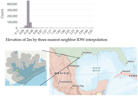
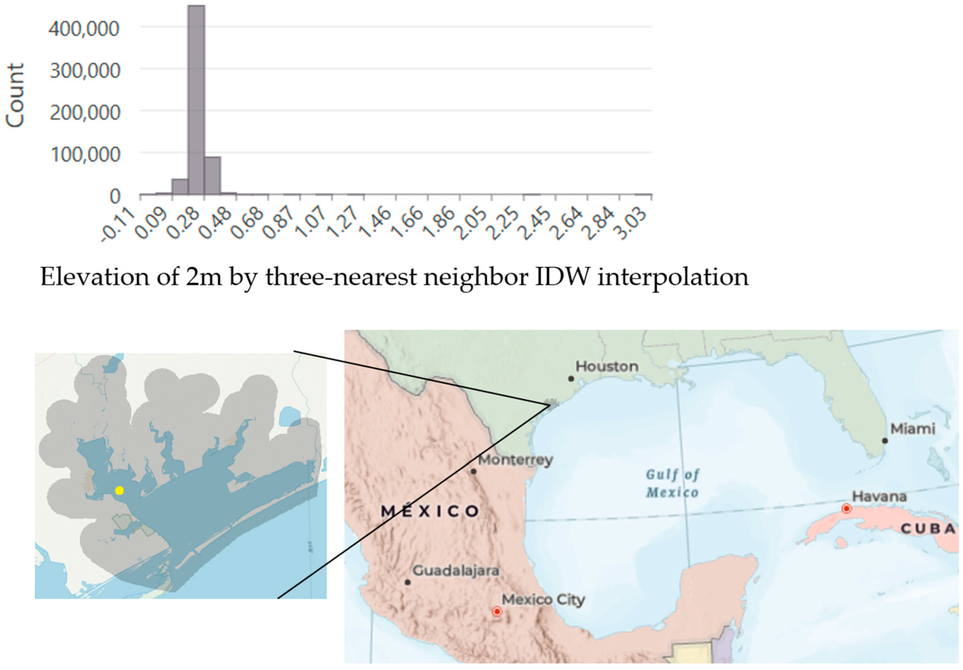
Figure 2 presents the histogram of water elevation in the study site’s water area. The mean water elevation is 0.247 m, with a skewness of 0.304. While a perfectly Gaussian distribution has a skewness of 0, values between −0.5 and 0.5 are generally considered to indicate approximate symmetry. Some lidar points recorded elevations of up to 3 m, likely corresponding to boats or flying seabirds—an occurrence commonly observed in coastal environments.
Figure 2.
Elevation histogram of a water area (yellow point on left picture) from extent (Top: 3,167,962 to 3,165,248; Left: 739,474 to 740,345) in the study site, which is on Texas Gulf Coast on right picture.
The choice of the threshold is empirical and based on visual examination of both the lidar data and WV2 imagery. This threshold operates as follows:
- (1)
- Water pixels with elevation higher than are assigned to non-water. Subsequent noise and artifact reduction steps suppressed isolated mislabeled pixels by reassigning clusters smaller than 7 pixels back to water. If these clusters actually represented water, the correction is appropriate; otherwise, the misclassification persists.
- (2)
- Land pixels with elevation lower than were assigned to water, though this misclassification was generally rare and remained uncorrected at this step.
This low occurrence is attributable to the timing of data acquisition. The lidar data were acquired in February 2018 and 2019, when water levels in Matagorda Bay are typically at their annual minima. Winter tides are lower due to astronomical factors: the Earth’s greater distance from the sun reduces solar tidal influence, resulting in weaker gravitational pulls and lower tides in the Northern Hemisphere [17]. In addition, according to NOAA Tides and Currents, low-tide conditions can approach −0.38 m relative to mean lower low water (MLLW).
Although strong north winds frequently push water out of Matagorda Bay into the Gulf of Mexico, causing exceptionally low tides and exposing extensive the bay floor areas [36,42], lidar surveys are typically scheduled and conducted during periods of low wind. As a result, the thresholding cannot take advantage of the low-water conditions caused by strong north winds.
3.5.5. Validation Points
For validation, we randomly generated points within regions defined as the area landward of a 60 m buffer along the initial water classification and the area waterward of the C-CAP reliable water boundary. These regions corresponded to the water expansion area, excluding C-CAP reliable water. Our classification method was also applied within these regions.
In the simplest scenario, where the following three polylines, (1) the water boundary of CCAP water class, (2) the water boundary of the initial water classification, and (3) the shoreline derived from thresholding the lidar elevation, were exactly aligned, the landward boundary of the validation regions was the edge of the water expansion, which expanded 60 m inland from the initial water blocks. The waterward boundary was defined by the C-CAP water boundary after shrinking 100 m. As a result, the water proportion of the validation regions is 62%, calculated as 100/(100 + 60). In Table 1 and Table 2, water points comprised roughly 57% of all samples, which corresponded well with their proportional area. It was acceptable that the water area exceeded the land area, as our approach begins with C-CAP reliable water and identifies white foam and wave crests over all likely areas, specifically between the outer 60 m buffer and C-CAP reliable water boundary.
Table 1.
Error matrix of the WV2 initial water classification.
Table 2.
Error matrix of the water classification.
To ensure spatial independence of validation samples, all points were spaced at least 50 m apart. Each validation sample was manually classified by referencing 2022 oblique imagery acquired with Pictometry camera systems (manufactured by Pictometry International, Rochester, NY, USA, and provided by from EagleView Technologies Rochester, NY, USA), Google Maps pre-2022, and also the WV2 imagery and the lidar data.
The same validation samples were applied on the WV2 initial water classification, and we have an accuracy assessment as following Table 1. Incorporating lidar elevation data to refine the initial WV2 classification resulted in an approximate 7% increase in accuracy.
Columns of the error matrix represent the reference data. Its rows represent the predicted data. F1-score and kappa coefficient of the water classification are 0.91 and 0.84, respectively.
3.5.6. Time and Space Complexity
The time complexity of applying a 3 × 3 filter over a N×M matrix is O(9×N×M) = O(N×M). When such filter is applied K times, the complexity becomes O(K×9×N×M), which still simplifies to O(N×M) since K and 9 are constants. The time complexities of lidar elevation statistics and local thresholding are O(1×N×M) for mean, O(1×N×M) for variance, and O(1×N×M) for local thresholding, respectively. All of these operations are linear with respect to the number of pixels.
DSM interpolation is I/O-intensive. Our three-nearest neighbor inverse distance weighting (3-NN IDW) interpolation requires only one read operation. The time complexity for reading and calculating distances for the nearest neighbors is O(number of points in a LiDAR tile). After reading a tile, we perform interpolation for each raster pixel, so for a raster of size W×L pixels, the complexity is O(W×L) for interpolation. After reading a tile, we perform interpolation for each raster pixel, so for a raster of size W × L pixels, the complexity is O(W×L) for interpolation.
However, since I/O costs are generally much higher than in-memory operations, the overall time complexity is dominated by the I/O, i.e., O(number of points in a lidar tile). Once all tiles have been read and interpolated, they are mosaicked into a larger N×M raster.
In summary, the total time complexity is
- (1)
- O(N×M) for in-memory processing;
- (2)
- [Number of tiles] × O(number of points in a LiDAR tile) for I/O costs.
Space complexity is O(N×M), since only eight intermediate matrices are maintained at any time: (1) initial water block, (2) C-CAP water, (3) water CCL, (4) water CCL area, (5) water expansion, (6) water intersection, (7) DSM, and (8) water classification.
4. Results and Discussions
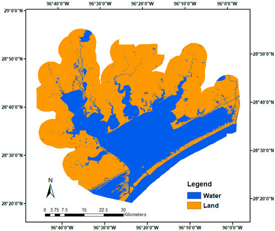
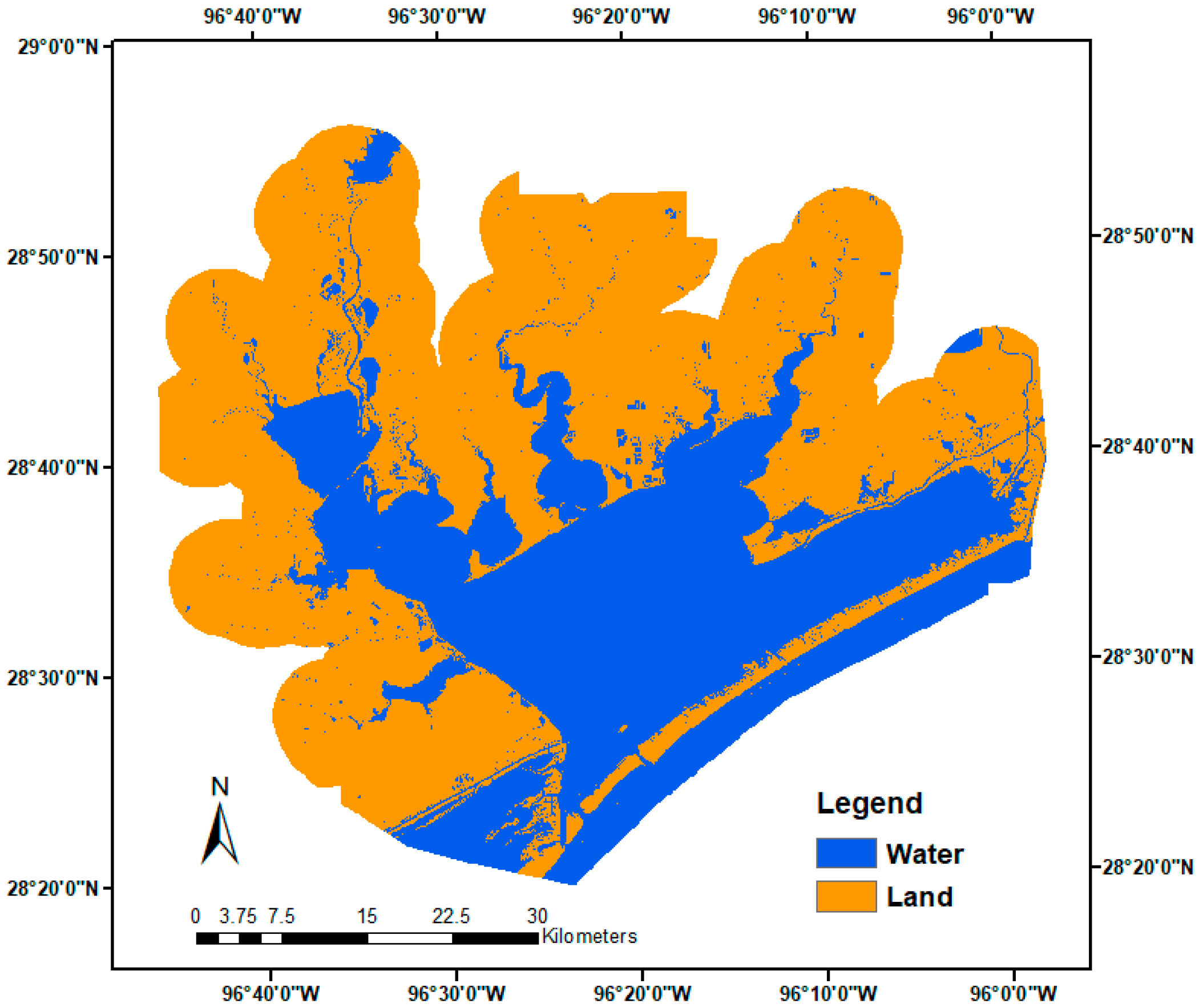
The final water–land classification map is depicted in Figure 3. We then used 1060 randomly located points (pixels) to assess the accuracy of the classifications (Table 2). The proposed classification approach that separates water and non-water gave promising results. The user’s, producer’s and total accuracies were 98.4%, 97.7%, and 97.7%, respectively, demonstrating the capability of our approach.
Figure 3.
Final water–land classification map of the Matagorda Bay region, Texas. Detail for right rectangle shown in Figure 4.
Columns of the error matrix represent the reference data. Its rows represent the predicted data. Producer’s accuracy measures the probability that a specific land cover on the ground is correctly classified. It is calculated as correctly classified samples for a class divided by total reference samples for that class. User’s accuracy indicates the probability that a class predicted on the map matches the reference. It is calculated as correctly classified samples divided by total samples classified as that class. User’s accuracy is to assess how reliable a class is from the user’s perspective. F1-score and kappa coefficient of the water classification are 0.98 and 0.95, respectively.
Our approach is the first to obtain an initial water classification by NDWI thresholding on high-resolution satellite images. NDWI can enhance water information efficiently in most cases. Typically, NDWI values above 0.2 indicate water bodies, while built-up features fall between 0 and 0.2. Zero or negative NDWI values correspond to vegetation and soil. It is not surprising that water turbidity, submerged aquatic vegetation, and bottom features of shallow water can shift the NDWI values in estuarine and coastal zones compared to those in clear deep water [37]. In addition to sun and sensor geometry, atmospheric conditions, and spectral characteristics of the observed surface objects, pixel mixing can also cause shifts in thresholds. Consequently, the initial water classification may contain mislabeling.
The second stage essentially is data localization. In other words, we partition the working extent into non-overlapping areas. Naturally, water-level varies in the semi-enclosed bays, primarily driven by offshore sea level fluctuations and local wind patterns, which are further modulated by bay geometry and bathymetry [17,36]. The water level spatial variability results in inconsistency in the height of lidar point clouds across the whole study site. To address this, partitioning the area allows us to use local thresholding and statistics to correct the initial water mislabeling. This partitioning process is independent on satellite images and lidar point clouds; instead, it is solely determined by the proximity to the initial water bodies.
Our third phase consists of two components: (1) utilizing existing land cover data to identify reliable water areas and (2) computing statistics based on these reliable waters. Here we have two assumptions, (1) we have reliable water areas and (2) local water-level change is minimal, allowing the preceding partition to tolerate some errors. Given that open waters in the bays have experienced little change since the 2016 C-CAP mapping, we can consider water areas to be stable. Additionally, the tidal range on the Gulf is low [37], suggesting that local water-level variations are small in the absence of strong winds and storm surges. Airborne lidar surveys usually avoid severe weather conditions. Therefore, it is reasonable to apply the local statistics to refine the initial water classification for each partitioned region.
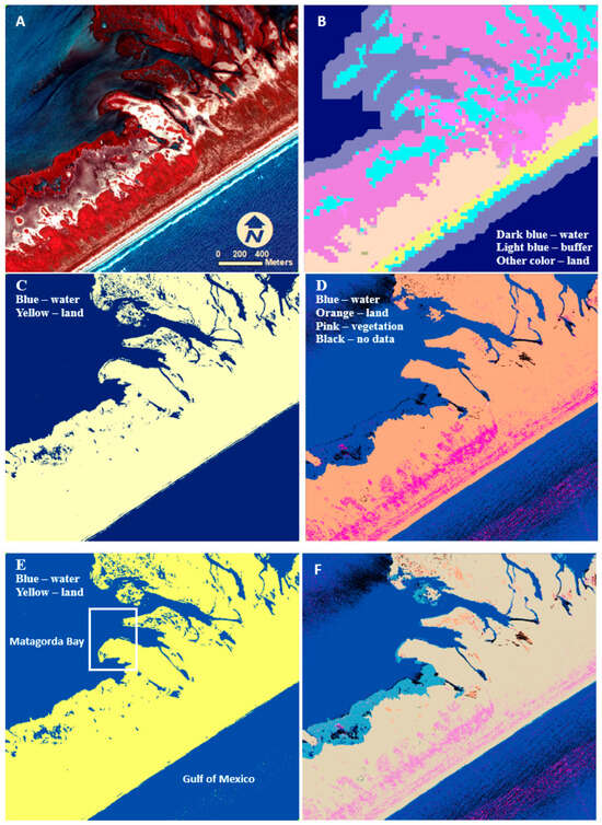
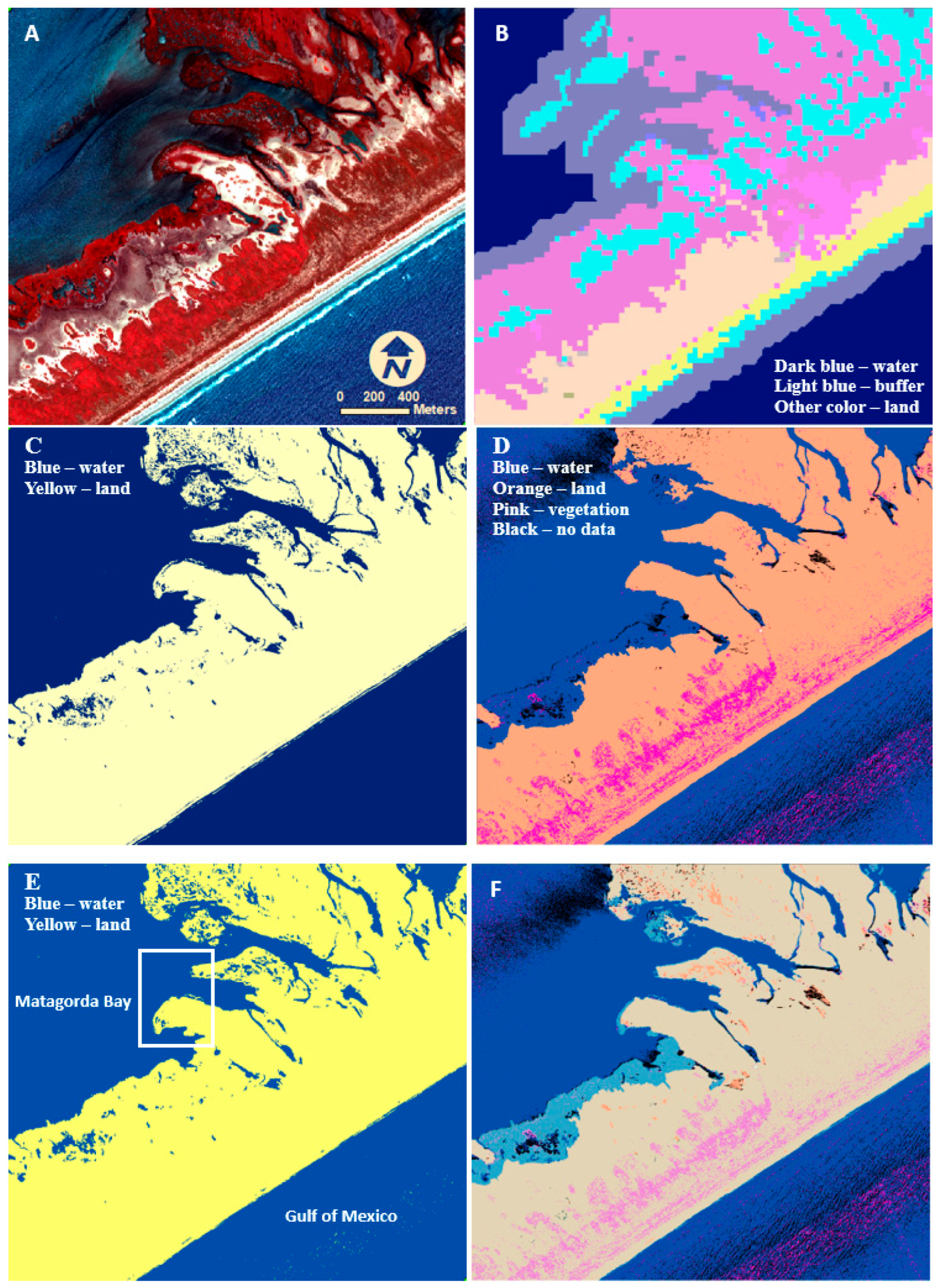
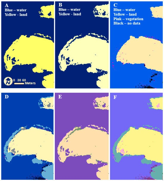
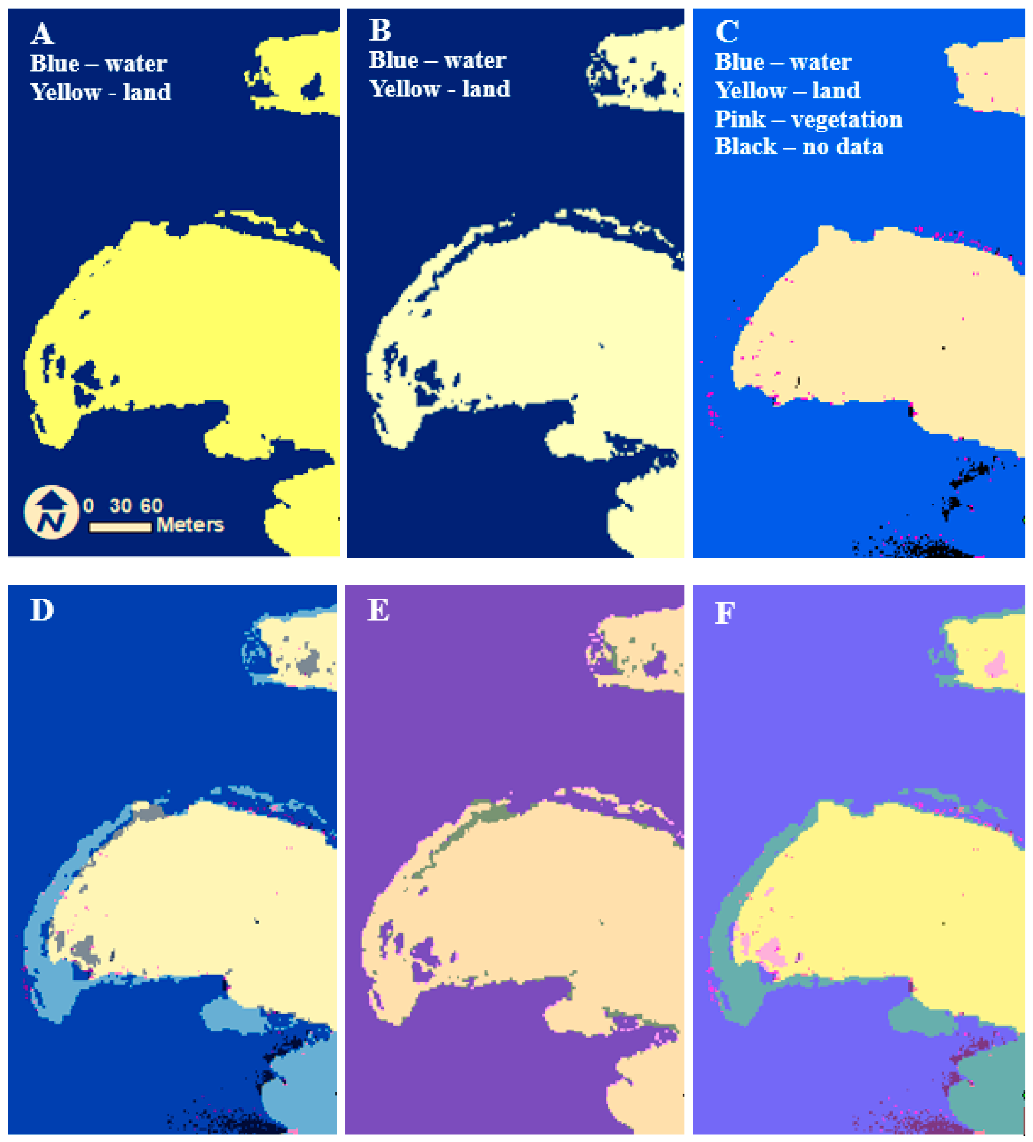
The six images on Figure 4 show the details of the water classification. By lidar data used in this study, the gulf water was 0.05 m higher than the bay water, and the fluctuation range of gulf water was over 0.2 m within the region shown on Figure 4. Moreover, the isolated waters on the barrier island could reach 0.4 m higher than the bay water. The WV2 CIR image (Figure 4A) provides a baseline for visual examination. Within Figure 4B, light blue represents water according to C-CAP classification, while dark blue denotes water shrunk 100 m from the preceding water. After shrinking, it is apparent that water is distanced from land, allowing us to avoid discrepancies between the C-CAP dataset and the WV2 image and lidar point clouds. Figure 4C represents the WV2 initial water classification. Figure 4D represents the original lidar point cloud classifications, and, notably, many areas are marked as no-data areas on water due to the low reflectance of water, resulting in insufficient energy returned from some water to the lidar sensor. Additionally, some waves are mislabeled as vegetation due to the fluctuating surface of waves. Apparently, the mislabeled vegetation is much more frequent on the gulf than on the bay because the bay water generally is calmer than the gulf water.
Figure 4.
Depiction of the progression of water classification for a section of Matagorda Peninsula, Texas. (A) WV2 imagery represented in false color by using the near infrared, red and green spectral bands mapped to RGB. (B) C-CAP classification after the 100 m shrink. (C) WV2 initial water classification. (D) Original lidar point cloud classification. (E) Final water classification. (F) Our water classification E overlapping with the original label of lidar point D with a transparency of 50%.
Lastly, Figure 4F compares the final water classification (Figure 4E) with the original lidar point cloud (Figure 4D). Notably, the no-data areas and most mislabeled vegetation areas in bay and gulf water have been corrected. Some mislabeled vegetation areas remain due to their size being larger than the size of salt–pepper filters. It also indicates that we did not simply use prior C-CAP water to assign labels for the pixels. Some large continuous areas (coral blue) on bayside that were classified as water from the lidar point clouds are assigned land by our approach. The same corrections also occur along the gulf beach. Their width is much narrower than bayside ones, because tidal flats on bayside are much wider than the beach on the gulf. The low reflectance of both wet soils easily leads to the assignment of water by lidar data providers. Those scattered yellow areas that were classified as land from the lidar point clouds are assigned water by our approach.
Figure 5 provides a detailed view of the region marked by the white rectangle in Figure 4E. In Figure 5D, the WV2 initial water classification (Figure 5B) is overlaid onto the original lidar point labels (Figure 5C). The land identified by the initial water classification from the WV2 multi-spectral image (depicted in light blue) extends significantly beyond the land identified by the lidar points towards the water. Some areas are classified as water in the initial water classification but not in the original lidar point labels (gray color), while all no-data areas from the original lidar point labels are classified as water in the initial water classification (black color), which is expected since no-data areas of lidar point clouds typically occur over water.
Figure 5.
Water classifications. (A) Final water classification. (B) Initial water classification obtained through WV2 NDWI. (C) Original lidar point cloud classifications. (D) The initial water classification (B) overlapping the original lidar point cloud classifications (C). (E) Final water classification (A) overlapping the initial water classification (B). (F) Final water classification (A) overlapping the original lidar point cloud classification (C). The overlapping is displayed with a transparency of 50%.
Within Figure 5E, the final water classification (Figure 5A) was overlaid onto the initial WV2 water classification (Figure 5B). Similarly, within Figure 5F, the final water classification (Figure 5A) was overlaid the lidar point labels (Figure 5C). Here, the green areas represent areas classified as water within the lidar points but land within the final classification, whereas the pink areas represent areas classified as land within the lidar points but water in the final classification. Two types of corrections are observed: transitioning from water to land in the final classification, and vice versa. These corrections are evident in both the WV2 data and the lidar point labels. Visual inspection and the total accuracy of 97.7% demonstrate that our final classification enhances the accuracy of both the initial water classification and the original labels of lidar points.
This experiment at Matagorda Bay, Texas, with approximately 2449 km2 area covered by 26 WorldView-2 images and 1568 lidar tiles demonstrated that the water–land maps are sufficiently accurate for assessing the biological and physical characteristics of the estuary.
The experiment shows that incorporating lidar elevation data to refine the initial WV2 classification resulted in an approximate 7% increase in accuracy. In addition to point elevation, point density and intensity offer valuable information for distinguishing between water and land, as well as for further classifying vegetation and bare earth. In future research, we would incorporate point density and intensity to improve classification accuracy.
5. Conclusions
This experiment focused on Matagorda Bay, Texas, demonstrates the concise and productive nature of our approach. By independently utilizing WV2 images and lidar point clouds, the temporal differences in the two datasets do not affect their efficacy. Due to using existing land cover data such as C-CAP to generate water statistics, this approach eliminates costly and time-consuming collection of training sets. The data localization achieved through non-overlapping partitioning allows this approach to handle waters with varying elevations from local water statistics. Ultimately, by capitalizing on the strengths of both satellite imagery and airborne lidar point clouds, our approach efficiently and accurately separates water and land for coastal zones. This approach is particularly feasible in situations where resources are insufficient for manual digitization or for creating a comprehensive training dataset required for deep learning methods.
Author Contributions
Conceptualization, L.S.; writing—original draft preparation, L.S.; writing—review and editing, J.M. and J.G.; funding acquisition, J.G. All authors have read and agreed to the published version of the manuscript.
Funding
This research was partially funded through NOAA award number NA21NOS4780147-T1-01 as part of NCCOS’s Effects of Sea Level Rise (ESLR) Program and the Texas Office of the Comptroller (Contract CMD 19-6799CS) by project Matagorda Bay Ecosystem Assessment Overview and Synopsis. The APC was funded by Texas A&M University-Corpus Christi.
Data Availability Statement
Data is available upon request from the authors. Or you can search “Matagorda Bay Ecosystem Assessment” and download data on GRIIDC (Gulf Science Data Repository).
Conflicts of Interest
The authors declare no conflicts of interest. Author Jessica Magolan was employed by the company Lynker Corporation. The remaining authors declare that the research was conducted in the absence of any commercial or financial relationships that could be construed as a potential conflict of interest.
Abbreviations
The following abbreviations are used in this manuscript:
| C-CAP | Coastal Change Analysis Program |
| NDWI | Normalized Difference Water Index |
| RGB | Red–Green–Blue |
| 3D | Three-Dimensional |
| NAD83 | North American Datum of 1983 |
| UTM | Universal Transverse Mercator |
| NAVD88 | North American Vertical Datum of 1988 |
| NIR | Near-Infrared |
| CIR | Color-Infrared |
| WV2 | WorldView 2 |
References
- Levin, P.S.; Fogarty, M.J.; Murawski, S.A.; Fluharty, D. Integrated ecosystem assessments: Developing the scientific basis for ecosystem-based management of the ocean. PLoS Biol. 2009, 7, e1000014. [Google Scholar] [CrossRef] [Scilit]
- Christensen, N.L.; Bartuska, A.M.; Brown, J.H.; Carpenter, S.; d’Antonio, C.; Francis, R.; Franklin, J.F.; MacMahon, J.A.; Noss, R.F.; Parsons, D.J.; et al. The report of the Ecological Society of America committee on the scientific basis for ecosystem management. Ecol. Appl. 1996, 6, 665–691. [Google Scholar] [CrossRef] [Scilit]
- Arkema, K.K.; Abramson, S.C.; Dewsbury, B.M. Marine ecosystem-based management: From characterization to implementation. Fron. Ecol. Environ. 2006, 4, 525–532. [Google Scholar] [CrossRef] [Scilit]
- Katsanevakis, S.; Stelzenmüller, V.; South, A.; Sørensen, T.K.; Jones, P.J.; Kerr, S.; Badalamenti, F.; Anagnostou, C.; Breen, P.; Chust, G.; et al. Ecosystem-based marine spatial management: Review of concepts, policies, tools, and critical issues. Ocean Coast. Manag. 2011, 54, 807–820. [Google Scholar] [CrossRef] [Scilit]
- Fernandino, G.; Elliff, C.I.; Silva, I.R. Ecosystem-based management of coastal zones in face of climate change impacts: Challenges and inequalities. J. Environ. Manag. 2018, 215, 32–39. [Google Scholar] [CrossRef] [Scilit]
- Su, L.; Magolan, J.; Gibeaut, J. Coastal Water Land Classification by Fusion of Satellite Imagery and Lidar Point Clouds. In Proceedings of the IGARSS 2023—2023 IEEE International Geoscience and Remote Sensing Symposium, Pasadena, CA, USA, 16–21 July 2023; pp. 4124–4126. [Google Scholar] [CrossRef] [Scilit]
- Liu, J.K.; Li, R.; Deshpande, S.; Niu, X.; Shih, T.Y. Estimation of Blufflines Using Topographic Lidar Data and Orthoimages. Photogramm. Eng. Remote Sens. 2009, 75, 69–79. [Google Scholar]
- Lee, I.S.; Park, H.J.; Lee, J.O.; Kim, Y.S. Delineating the Natural Features of a Cadastral Shoreline in South Korea Using Airborne Laser Scanning. IEEE J. Sel. Top. Appl. Earth Obs. Remote Sens. 2011, 4, 905–910. [Google Scholar] [CrossRef] [Scilit]
- Yousef, A.; Iftekharuddin, K. Shoreline extraction from the fusion of LiDAR DEM data and aerial images using mutual information and genetic algorithms. In Proceedings of the 2014 International Joint Conference on Neural Networks, Beijing, China, 6–11 July 2014; pp. 1007–1014. [Google Scholar] [CrossRef] [Scilit]
- Yang, T.; Jiang, S.; Hong, Z.; Zhang, Y.; Han, Y.; Zhou, R.; Wang, J.; Yang, S.; Tong, X.; Kuc, T. Sea-Land Segmentation Using Deep Learning Techniques for Landsat-8 OLI Imagery. Mar. Geod. 2022, 43, 105–133. [Google Scholar] [CrossRef] [Scilit]
- Klemas, V. Remote Sensing Techniques for Studying Coastal Ecosystems: An Overview. J. Coast. Res. 2011, 27, 12–17. [Google Scholar]
- Huang, C.; Chen, Y.; Zhang, S.; Wu, J. Detecting, extracting, and monitoring surface water from space using optical sensors: A review. Rev. Geophys. 2018, 56, 333–377. [Google Scholar] [CrossRef] [Scilit]
- Li, Y.; Dang, B.; Zhang, Y.; Du, Z. Water body classification from high-resolution optical remote sensing imagery: Achievements and perspectives. ISPRS J. Photogramm. Remote Sens. 2022, 187, 306–327. [Google Scholar] [CrossRef] [Scilit]
- Sun, D.; Gao, G.; Huang, L.; Liu, Y.; Liu, D. Extraction of water bodies from high-resolution remote sensing imagery based on a deep semantic segmentation network. Sci. Rep. 2024, 14, 14604. [Google Scholar] [CrossRef] [Scilit] [PubMed]
- White, S.; Parrish, C.; Calder, B.; Pe’eri, S.; Rzhanov, Y. Lidar-derived national shoreline: Empirical and stochastic uncertainty analyses. J. Coast. Res. 2011, 62, 62–74. [Google Scholar] [CrossRef] [Scilit]
- Song, H.; Jung, J. A Fully Automated and Scalable Surface Water Mapping with Topographic Airborne LiDAR Data. arXiv 2023, arXiv:2301.06567. [Google Scholar]
- The Open University. Waves, Tides and Shallow Water Processes, 2nd ed.; Butterworth-Heinemann: Oxford, UK, 1999; 227p. [Google Scholar]
- Mann, K.H. Ecology of Coastal Waters: With Implications for Management, 2nd ed.; Wiley-Blackwell: Hoboken, NJ, USA, 2009. [Google Scholar]
- Su, L.; Gibeaut, J. Extracting Surface Features of the Nueces River Delta Using Lidar Points. In Proceedings of the ASPRS/MAPPS 2009 Fall Conference, San Antonio, TX, USA, 16–19 November 2009. [Google Scholar]
- Lin, Y.; Yan, L.; Tong, Q. Automatic recognition of rivers from lidar data by profile factor. Int. Arch. Photogramm. Remote Sens. Spat. Inf. Sci. 2008, 37, 245. [Google Scholar]
- Baruch, A.; Filin, S. Detection of gullies in roughly textured terrain using airborne laser scanning data. ISPRS J. Photogramm. Remote Sens. 2011, 66, 564–578. [Google Scholar] [CrossRef] [Scilit]
- Höfle, B.; Vetter, M.; Pfeifer, N.; Mandlburger, G.; Stötter, J. Water surface mapping from airborne laser scanning using signal intensity and elevation data. Earth Surf. Process. Landf. 2009, 34, 1635–1649. [Google Scholar] [CrossRef] [Scilit]
- Brzank, A.; Heipke, C.; Goepfert, J.; Soergel, U. Aspects of Generating Precise Digital Terrain Models in the Wadden Sea from Lidar–Water Classification and Structure Line Extraction. ISPRS J. Photogramm. Remote Sens. 2008, 63, 510–528. [Google Scholar] [CrossRef] [Scilit]
- Irwin, K.; Beaulne, D.; Braun, A.; Fotopoulos, G. Fusion of SAR, Optical Imagery and Airborne LiDAR for Surface Water Detection. Remote Sens. 2017, 9, 890. [Google Scholar] [CrossRef] [Scilit]
- Shaker, A.; Yan, W.Y.; LaRocque, P.E. Automatic land-water classification using multispectral airborne LiDAR data for near-shore and river environments. ISPRS J. Photogramm. Remote Sens. 2019, 152, 94–108. [Google Scholar] [CrossRef] [Scilit]
- Smeeckaert, J.; Mallet, C.; David, N.; Chehata, N.; Ferraz, A. Large-scale classification of water areas using airborne topographic lidar data. Remote Sens. Environ. 2013, 138, 134–148. [Google Scholar] [CrossRef] [Scilit]
- Lee, I.C.; Wu, B.; Li, R. Shoreline extraction from the integration of lidar point cloud data and aerial orthophotos using mean-shift segmentation. In Proceedings of the ASPRS Annual Conference, Baltimore, MA, USA, 9–13 March 2009; pp. 3033–3040. [Google Scholar]
- Miura, Y.; Shamsudduha, M.; Suppasri, A.; Sano, D. A Global Multi-Sensor Dataset of Surface Water Indices from Landsat-8 and Sentinel-2 Satellite Measurements. Sci. Data 2025, 12, 1253. [Google Scholar] [CrossRef] [Scilit]
- Man, G.; Yun, Q.; Qilin, Z.; Yuyong, L.; Zhuoshi, Z. Surface water quality classification and prediction model based on multiple machine learning algorithms. Sci. Rep. 2025, 15, 39907. [Google Scholar] [CrossRef] [Scilit] [PubMed]
- Isikdogan, F.; Bovik, A.C.; Passalacqua, P. Surface Water Mapping by Deep Learning. IEEE J. Sel. Top. Appl. Earth Obs. Remote Sens. 2017, 10, 4909–4918. [Google Scholar] [CrossRef] [Scilit]
- Mullen, A.L.; Watts, J.D.; Rogers, B.M.; Carroll, M.L.; Elder, C.D.; Noomah, J.; Williams, Z.; Caraballo-Vega, J.A.; Bredder, A.; Rickenbaugh, E.; et al. Using high-resolution satellite imagery and deep learning to track dynamic seasonality in small water bodies. Geophys. Res. Lett. 2023, 50, e2022GL102327. [Google Scholar] [CrossRef] [Scilit]
- National Oceanic and Atmospheric Administration, Office for Coastal Management. “2016 NOAA C-CAP Regional Land Cover.” Coastal Change Analysis Program (C-CAP) Regional Land Cover; NOAA Office for Coastal Management: Charleston, SC, USA, 2016. Available online: www.coast.noaa.gov/htdata/raster1/landcover/bulkdownload/30m_lc/ (accessed on 1 May 2023).
- McFeeters, S.K. The use of the Normalized Difference Water Index (NDWI) in the delineation of open water features. Int. J. Remote Sens. 1996, 17, 1425–1432. [Google Scholar] [CrossRef] [Scilit]
- Gonzalez, R.C.; Woods, R.E.; Eddins, S.L. Digital Image Processing Using MATLAB, 3rd ed.; Gatesmark Publishing: Knoxville, TN, USA, 2020. [Google Scholar]
- Samet, H.; Tamminen, M. Efficient Component Labeling of Images of Arbitrary Dimension Represented by Linear Bintrees. IEEE Trans. Pattern. Anal. Mach. Intell. 1988, 10, 579–586. [Google Scholar] [CrossRef] [Scilit]
- Davis, R.A. Sediments of the Gulf of Mexico. In Habitats and Biota of the Gulf of Mexico: Before the Deepwater Horizon Oil Spill; Ward, C.H., Ed.; Springer: New York, NY, USA, 2017; pp. 165–215. [Google Scholar] [CrossRef] [Scilit]
- Su, L.; Huang, Y. Seagrass Resource Assessment using WorldView-2 Imagery in the Redfish Bay, Texas. J. Mar. Sci. Eng. 2019, 7, 98. [Google Scholar] [CrossRef] [Scilit]
- Micijevic, E.; Rengarajan, R.; Haque, M.O.; Lubke, M.; Tuli, F.T.; Shaw, J.L.; Hasan, N.; Denevan, A.; Franks, S.; Choate, M.J.; et al. ECCOE Landsat Quarterly Calibration and Validation Report—Quarter 2, 2021; U.S. Geological Survey Open-File Report 2021-1105; U.S. Geological Survey: Reston, VA, USA, 2021; 40p. [CrossRef] [Scilit]
- Paine, J.G.; Caudle, T.L. Shoreline Movement Along the Texas Gulf Coast, 1930s to 2019, Bureau of Economic Geology, The University of Texas at Austin (Texas General Land Office, Contract No. 16-201-000, April 2020). Available online: https://www.beg.utexas.edu/files/content/beg/research/gulfShorelineUpdate2019_r03.pdf (accessed on 23 March 2026).
- Saylam, K.; Hupp, J.R.; Andrews, J.R.; Averett, A.R.; Knudby, A.J. Quantifying Airborne Lidar Bathymetry Quality-Control Measures: A Case Study in Frio River, Texas. Sensors 2018, 18, 4153. [Google Scholar] [CrossRef] [Scilit] [PubMed]
- McKean, J.; Tonina, D.; Bohn, C.; Wright, C.W. Effects of bathymetric lidar errors on flow properties predicted with a multi-dimensional hydraulic model. J. Geophys. Res. Earth Surf. 2014, 119, 644–664. [Google Scholar] [CrossRef] [Scilit]
- Ross, D.A. Introduction to Oceanography; HarperCollins: New York, NY, USA, 1995; pp. 236–242. [Google Scholar]

Disclaimer/Publisher’s Note: The statements, opinions and data contained in all publications are solely those of the individual author(s) and contributor(s) and not of MDPI and/or the editor(s). MDPI and/or the editor(s) disclaim responsibility for any injury to people or property resulting from any ideas, methods, instructions or products referred to in the content. |
© 2026 by the authors. Licensee MDPI, Basel, Switzerland. This article is an open access article distributed under the terms and conditions of the Creative Commons Attribution (CC BY) license.