


Abstract
An accurate prediction of the short-term motion attitude of ships is essential for navigation safety and offshore operations. However, conventional time series prediction models have constraints in handling time-varying dynamics and adapting to diverse sea states. Therefore, Ship Motion Attitude Prediction Network (SMAPNet) based on Non-Symmetric Tri-Cube Kernel Trend Filter (NTKTF) is proposed in the present paper. SMAPNet decomposes temporal signals using the Feature Extraction Block (FEB), fuses local and global features through Feature Refinement Block (FRB), and integrates Bidirectional Long Short-Term Memory Network (Bi-LSTM) with a self-attention mechanism, Feature Prediction Block (FPB), for short-term prediction within 1 to 5 s. In this experiment, field-measured data from the ship XIN HONG ZHUAN were employed to construct online prediction scenarios, and a systematic evaluation was conducted from three perspectives: local prediction accuracy, evaluation metric, and error distribution. The findings indicate that SMAPNet exhibits improved adaptability and prediction accuracy in predicting ship motion attitudes under different sea states. Specifically, in the single-step prediction of roll and pitch under sea states 3 and 4, the mean square errors (MSE) of SMAPNet are reduced by 10.45%, 6.96% and 14.60%, 2.77% respectively compared with the superior candidate model.
1. Introduction
During navigation, ocean-going ships are subject to combined wind and wave disturbances, resulting in highly unpredictable and non-stationary motions with six degrees of freedom (6-DOF) [1]. These dynamic time-varying motions not only pose a serious threat to the safety of personnel, offshore operations, and the stability of shipboard equipment [2], but also affect the safety of shipborne helicopters during takeoff and landing [3] and the launch accuracy of shipborne weapons [4]. Among these motions, roll and pitch have a significant influence on ship stability [5]. Regarding safe and efficient navigation and various operational tasks, it is therefore essential to accurately predict a ship’s roll and pitch motions in the short term and integrate with motion compensation systems for mitigation [6].
Recent research has increasingly focused on accurate short-term estimation of ship motion attitude in the field of intelligent ships and ocean engineering. Short-term ship motion attitude prediction typically refers to real-time prediction, involving the forecast of future ship motion attitude over a period of several to ten-odd seconds [7]. There are currently two mainstream ship motion attitude prediction models: time series prediction models based on statistical theory [8] and intelligent models based on machine learning and deep learning [9].
A prediction model based on convolutional operations was designed to predict the ship motion attitude by taking the bow-generated wave height as input data and convolving it with the ship motion response function, featuring computationally intensive procedures and compromised accuracy. The statistical theory-based time series prediction model takes it as a core to construct a time series model using a ship’s historical attitude data. By directly extracting inherent patterns from historical data through statistical modeling, it eliminates reliance on solving complex dynamic equations which consequently simplifies the prediction process while ensuring the model’s lightweight nature and computational efficiency. However, models such as Kalman filter [10] autoregressive model (AR) [8], autoregressive moving average model (ARMA) [11], and autoregressive integrated moving average model (ARIMA) [12] depend on linear theory and demonstrate notable constraints in addressing the highly nonlinear and non-stationary characteristics of ship motion, complicating accurate predictions of the ship motion attitude.
Recent years have witnessed a significant popularity of machine learning (ML) methods such as support vector machine (SVM) [13], random forests [14], and neural networks [15] in predicting nonlinear and non-stationary ship motions. Yin et al. [16] overcame the limitations of inaccurate predictions by traditional empirical formulas at the detailed design stage using gray relational analysis and the SVM method. Chen et al. [17] estimated parameters for the ship’s roll response model in shallow water using the nonlinear least squares support vector machine (NLS-SVM) technique. Liong and Chua [18] analyzed the prediction of real-time deterministic ship motion using a hybrid artificial neural network (ANN) and Ensemble Kalman Filter (EnKF) approach, with difficulty in vanishing or exploding gradients under the condition of increased network depth or training on large datasets [19]. However, with the emergence of deep learning (DL) models such as recurrent neural networks (RNNs) and their variants possessing temporal sequence memory capabilities, the gradient vanishing and exploding issues have been efficiently lessened. Chen et al. [20] examined the real-time prediction of multi-degree-of-freedom motion and quiescent intervals of a ship using a Long Short-Term Memory (LSTM) Network, demonstrating the model’s substantially higher prediction accuracy compared with a conventional neural network model. Despite its superiority to numerous conventional neural network architectures in terms of efficacy [21], LSTM is restricted to unidirectional feature extraction along the temporal axis, undermining its capacity to grasp time-series characteristics and complicating the thorough exploitation of intricate properties inherent in time-series data. Bidirectional Long Short-Term Memory Network (Bi-LSTM) comprises two independent LSTM architectures [22], realizing deep feature extraction of sequences through bidirectional temporal processing. However, insufficient dynamic adaptive mechanism in Bi-LSTM makes it difficult to effectively extract feature information when facing strongly nonlinear and non-stationary ship motion attitude time series. Therefore, the use of hybrid algorithms has been considered to improve the model prediction [23]. Wang, et al. [24] developed a hybrid algorithmic model by combining Bi-LSTM with a one-dimensional convolutional neural network (1DCNN), so as to improve the accuracy of ship roll motion prediction by leveraging the feature extraction capabilities of convolutional layers to capture deep temporal dependencies. Zhang et al. [25] constructed a dual-branch parallel architecture combining 1DCNN and LSTM to predict ship roll motion data generated by CFD-based methods. Although CFD simulations can mitigate data scarcity issues in high-sea-state conditions, discrepancies exist between simulated and real ship motions. The model’s generalization capability in real-world marine environments requires further validation.
Although hybrid models can improve the prediction performance of ship motion attitude characterized by complex nonlinear behavior [26], recurrent neural networks and their variants may still be affected by disturbance-related high-frequency fluctuations and measurement noise when directly processing raw non-stationary sequences. When such raw signals are directly fed into the model, the recurrent structure may fit high-frequency disturbance components together with effective temporal information, which can increase local fluctuations in the predicted results and reduce prediction stability. Therefore, some researchers have introduced signal decomposition algorithms, such as Empirical Mode Decomposition (EMD) [27], into prediction models to preprocess non-stationary sequences before temporal feature learning. These methods decompose the original sequence into several sub-series or modal components with different time-scale characteristics, allowing the prediction model to learn simpler components while alleviating the adverse influence of high-frequency disturbances on the prediction results. Geng et al. [28] focused on the highly nonlinear and non-stationary characteristics in ship motion time series by integrating EMD with adaptive Particle Swarm Optimization-Long Short-Term Memory (PSO-LSTM) Networks. Compared with traditional neural network models, Empirical Mode Decomposition exhibits significantly higher accuracy in predicting ship motion attitude, but with insufficient decomposition robustness due to mode aliasing and noise sensitivity, and weak physical interpretability [28]. Zhang et al. [29] proposed a hybrid approach integrating Variational Mode Decomposition (VMD), Gated Recurrent Unit (GRU), and Error Correction (EC). VMD was utilized to separately decompose the non-stationary roll motion of training and testing datasets into stationary intrinsic mode functions (IMFs), exhibiting superior prediction performance. Although VMD can effectively suppress mode aliasing, the predetermined mode number K still relies on empirical selection, leading to over-decomposition or under-decomposition issues, coupled with high computational complexity. Xu and Yin [30] proposed an enhanced hybrid scheme for ship transverse rocking prediction, combining support vector regression (SVR), time-varying filter-based ensemble Empirical Mode Decomposition (TVF-EMD), and the improved black widow optimization algorithm (IBWOA). Specifically, TVF-EMD was used to decompose non-stationary ship transverse motion data into multiple mode components with dynamic time-varying characteristics, aiming to avoiding mode mixing and intermittency in the traditional Empirical Mode Decomposition (EMD); SVR was used to train and predict these mode components; IBWOA was used to optimize parameter configurations of TVF-EMD, thereby increasing the model’s prediction accuracy. These studies have improved the accuracy of ship motion attitude prediction through signal decomposition techniques, significantly superior to traditional neural network models. However, such method relies on decomposing the complete sequence of the training set or validation set, leading to the implicit inclusion of global data features in the sliding window when predicting future sequences, and underlying information leakage, which is also known as look-ahead bias in statistical forecasting [31]. Therefore, the technical route based on global sequence decomposition may limit the applicability of such methods in engineering scenarios.
To address the potential look-ahead bias caused by global sequence decomposition in existing decomposition-based prediction methods, this paper constructs a Ship Motion Attitude Prediction Network (SMAPNet) by integrating the Non-Symmetric Tri-Cube Kernel Trend Filter (NTKTF) with neural networks for short-term online prediction of ship roll and pitch motions. The proposed model consists of three functional modules: the Feature Extraction Block (FEB), Feature Refinement Block (FRB), and Feature Prediction Block (FPB). The main contributions of this study are summarized as follows:
- (1)
- An NTKTF-based FEB is designed for online decomposition of non-stationary ship motion attitude signals. The original roll or pitch sequence is decomposed into a trend component and a residual component using historical and current observations, reducing the dependence on global sequence decomposition.
- (2)
- A hybrid feature learning framework is constructed by integrating FEB, FRB, and FPB. The model combines NTKTF-based decomposition, 1DCNN-based local feature extraction, LSTM/Bi-LSTM-based temporal modeling, and self-attention-based feature refinement, enabling multi-level feature extraction from the original, trend, and residual components.
- (3)
- The proposed SMAPNet is validated using measured roll and pitch data from the ocean-going training ship XIN HONG ZHUAN under sea states 3 and 4. The model is evaluated from local prediction accuracy, quantitative evaluation metrics, error distribution, extended prediction horizon, and computational efficiency, demonstrating its effectiveness in short-term online ship motion attitude prediction.
The rest of this paper is organized as follows: Section 2 introduces the background knowledge of NTKTF, CNN, Bi-LSTM, and the self-attention mechanism. Section 3 presents the architecture of the proposed SMAPNet model. Section 4 describes the experimental setup, including data preprocessing, evaluation metrics, hyperparameter settings, and comparative models. Section 5 presents the experimental results and analysis. Section 6 concludes this paper and discusses future work.
2. Background Knowledge
2.1. Non-Symmetric Tri-Cube Kernel Trend Filter (NTKTF)
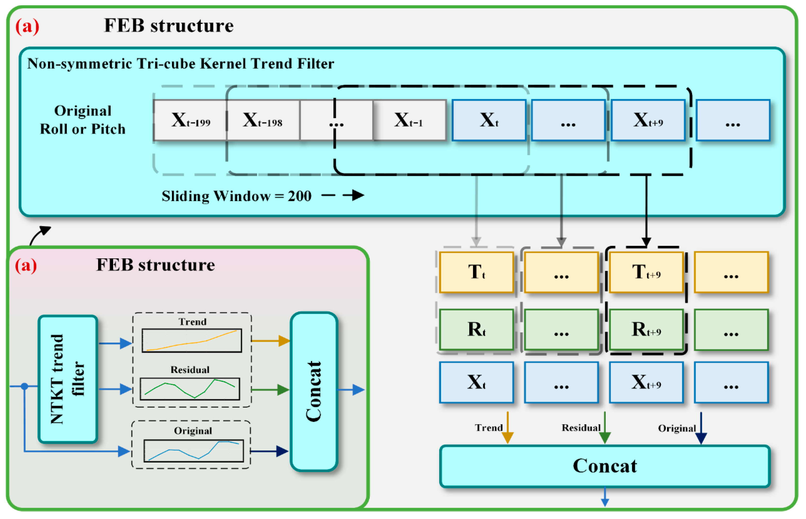
Non-Symmetric Tri-Cube Kernel Trend Filter (NTKTF) is a general time series trend extraction method based on the tri-cube kernel function asymmetric weighted smoothing [32], with the capability of online incremental updating and dynamic time-varying data adaptation. NTKTF is improved from the symmetric cubic kernel trend filter and can eliminate the use of future data for weighting calculations [33]. The NTKTF achieves dynamic estimation of the current trend by applying weights wi that decay nonlinearly over time to historical observations. The filter uses a sliding window of the length to store historical and recent observations, where denotes the observation at time . For each observation within the window, a tri-cubic kernel function is used to generate . The trend component is the weighted average of observations in the window. When a new observation arrives, the sliding window is updated to , and the trend component is recalculated. The difference between observed and trend components is the residual component , which can be regarded as a time-varying periodicities feature with a random noise component due to tides, wind, and waves. The formula for the NTKTF is shown in Equations (1)–(4).
where is the index of the observation within the sliding window, is the relative position parameter, is the sliding window size; is the cubic kernel function, is the s-decay weight, is the trend component, and is the residual component. The time complexity of this method is , whose computational cost stems mainly from the element-wise computation of and within the sliding window and the weighted summation operation of ; the linear complexity characteristic ensures its fast response to new observations in online scenarios.
In this study, NTKTF is applied separately to the roll or pitch attitude time series. Each sequence is decomposed into a trend component representing the slowly varying tendency and a residual component containing time-varying periodicities and disturbance-related fluctuations, thereby enhancing the model’s learning capability for ship motion attitude prediction.
2.2. Convolutional Neural Network (CNN)
CNN captures local features of data through automated feature extraction capability and derives global information by integrating highly correlated local patterns. Simultaneously, the implementation of weight sharing can significantly reduce model parameters and computational complexity, making CNNs particularly efficient in classification and recognition tasks during the data processing process [34]. One-dimensional convolutional neural network (1DCNN) performs a convolution operation by sliding a convolution kernel along the temporal dimension to extract edge features and intrinsic complex patterns from the data, while optimizing kernel parameters via backpropagation [35]. The mathematical formulation of the convolution operation dimensions is provided in Equation (5). Figure 1 illustrates the architecture of 1DCNN.
Figure 1.
Structure diagram of 1DCNN.
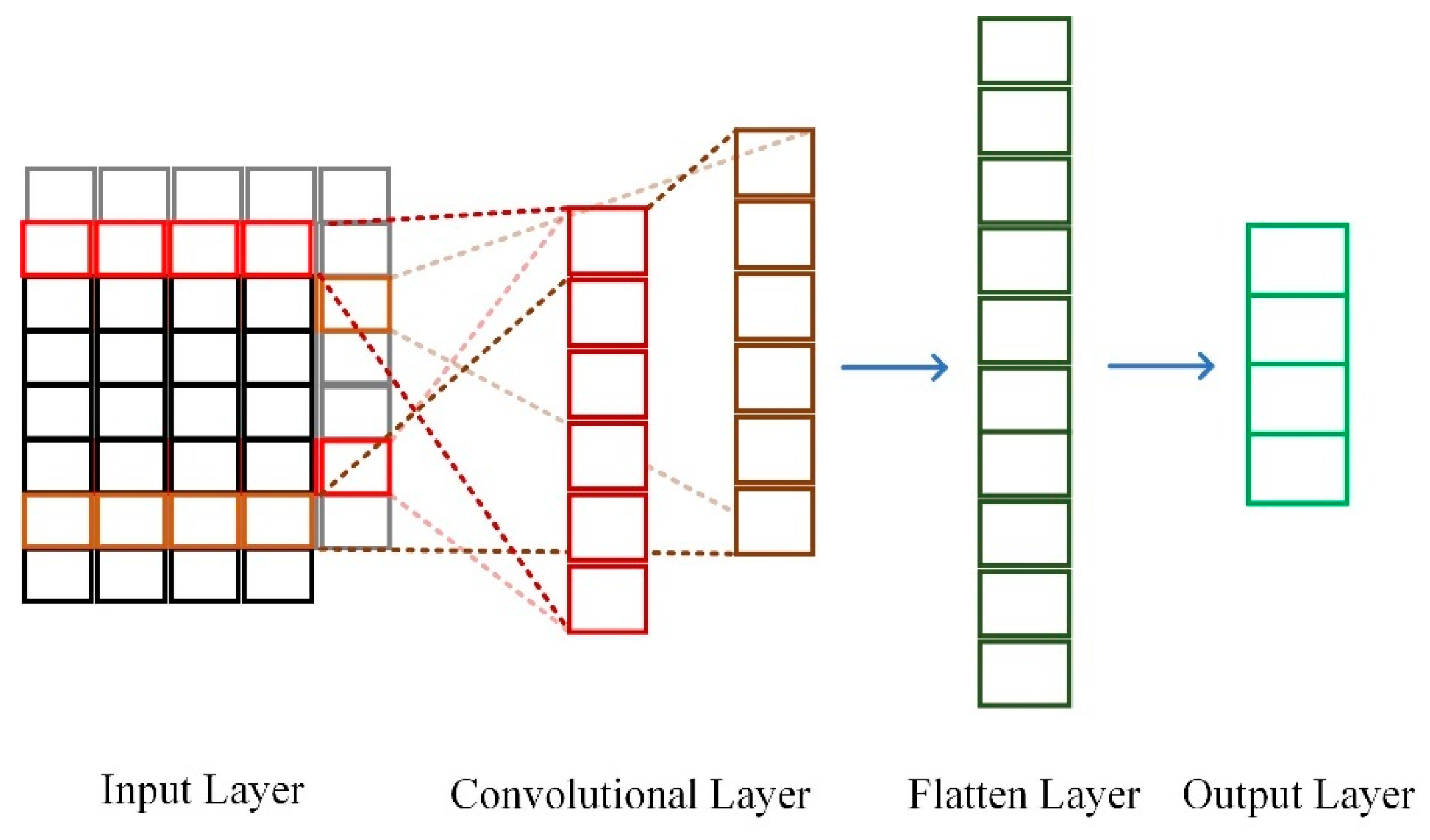
In the equation, represents the temporal dimension size of the convolutional layer’s output. denotes the temporal dimension size of the input tensor. is the kernel size along the temporal axis. is the padding size. is the stride of the convolutional kernel.
Short-term features within dynamic time-varying sequences can be effectively captured through the local receptive field capability of convolutional kernels in 1DCNN, thereby enhancing the model’s predictive capability for ship motion attitude.
2.3. Bidirectional Long and Short-Term Memory (Bi-LSTM)
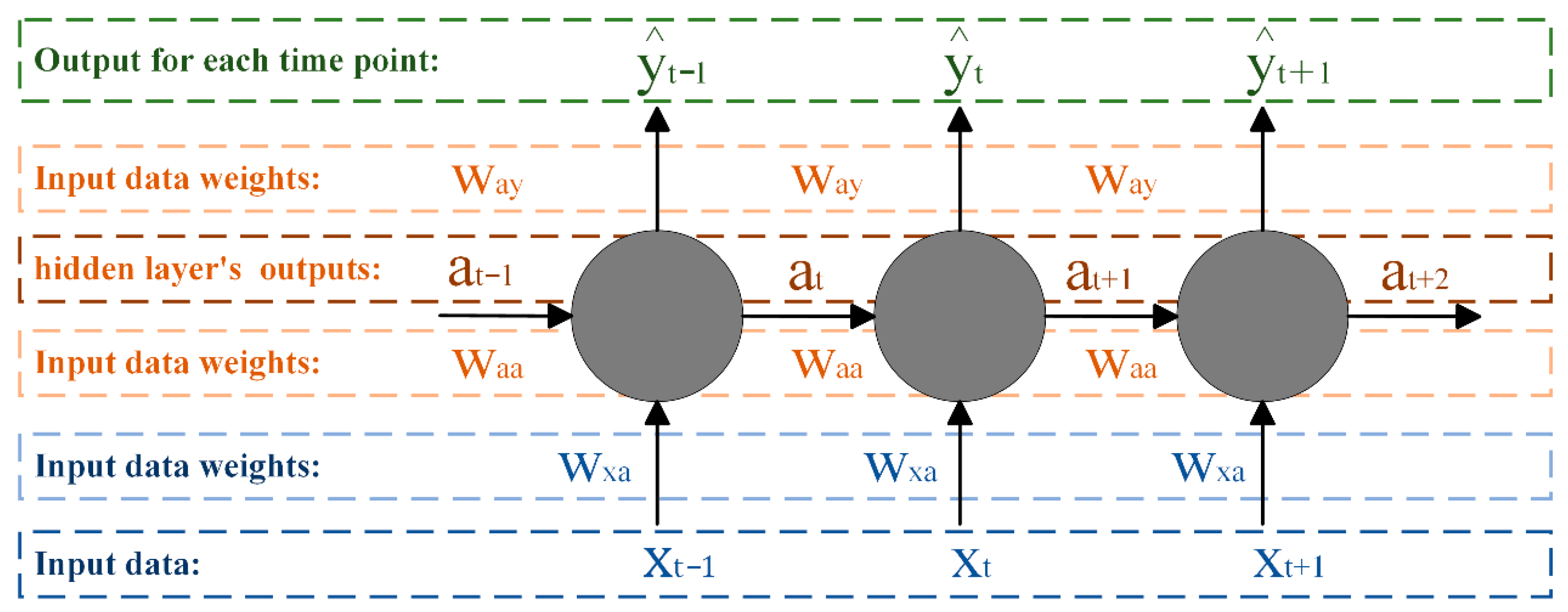
Bi-LSTM is a variant of the Recurrent Neural Network (RNN). The schematic diagram of the RNN structure is shown in Figure 2, and computational formulas for hidden and output layers in its network structure are provided in Equations (6) and (7).
where and are the outputs of hidden layer and output layer at time step t; , , are shared weight matrices; is the input at time step t; and are activation functions, with and being the bias vectors.
Figure 2.
Network structure of the RNN.
In RNNs, the data sequence with excessive length is prone to the vanishing gradient problem. Additionally, traditional RNNs can only utilize historical time step information to predict future time steps, without capturing the influence of future information on the current time step [36]. In the problem of ship motion attitude prediction, roll and pitch motions of a ship are influenced by both historical time steps and future time steps. Therefore, this paper employed a Bi-LSTM [37] to encode ship motion attitude data from both historical and future directions, leveraging both past and future information to jointly predict current ship motion attitude. As illustrated in Figure 3, input sequences are fed into forward and backward layers, respectively. The outputs from both layers are concatenated and processed through the output layer for prediction, yielding the Bi-LSTM hidden state . The relevant equations are provided in Equations (8)–(10).
Figure 3.
Network structure of the Bi-LSTM.
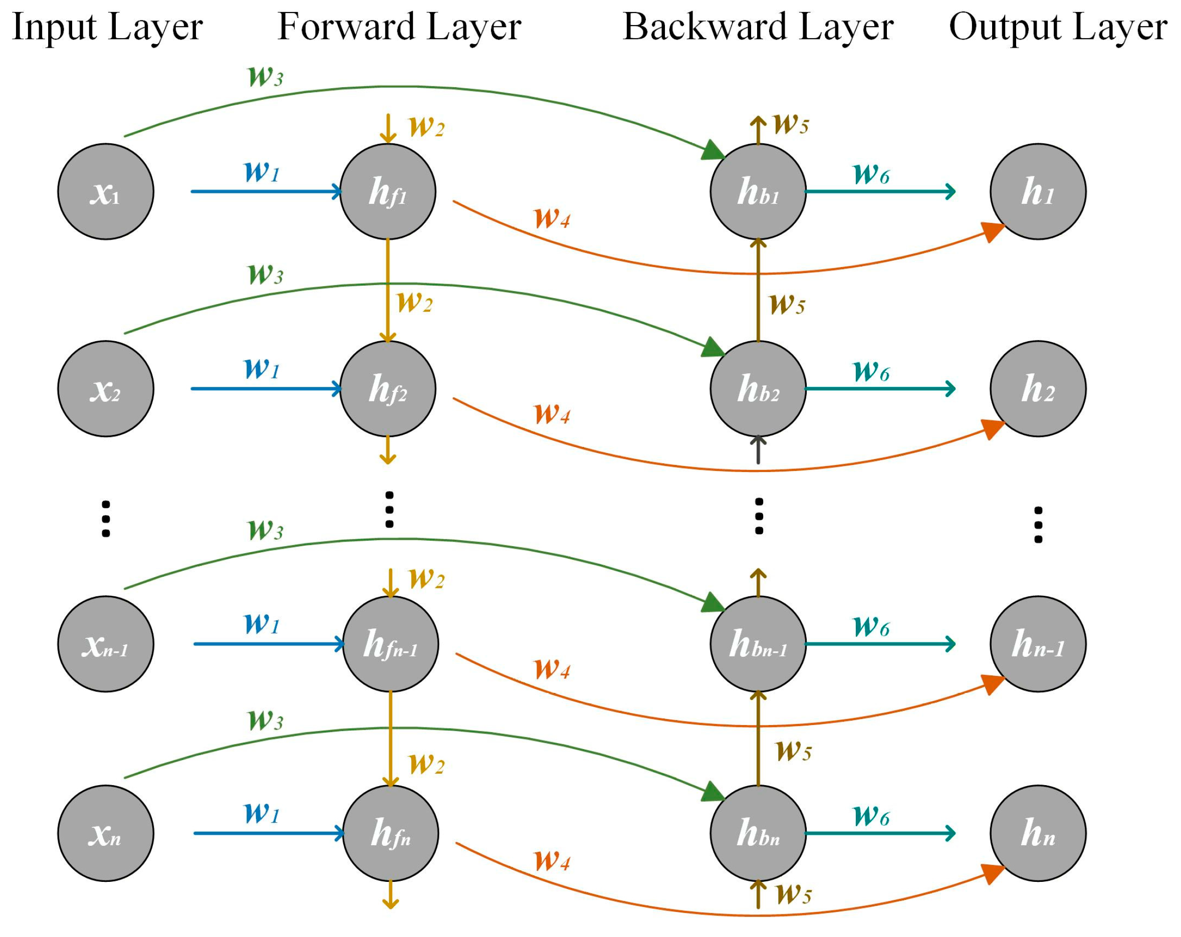
In the equation, are layer-wise shared weights, denotes the output of the forward memory unit, represents the output of the backward memory unit, and , , correspond to bias terms of the forward memory unit, backward memory unit, and output layer, respectively.
2.4. Self-Attention Mechanism
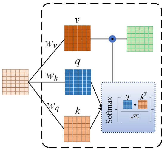
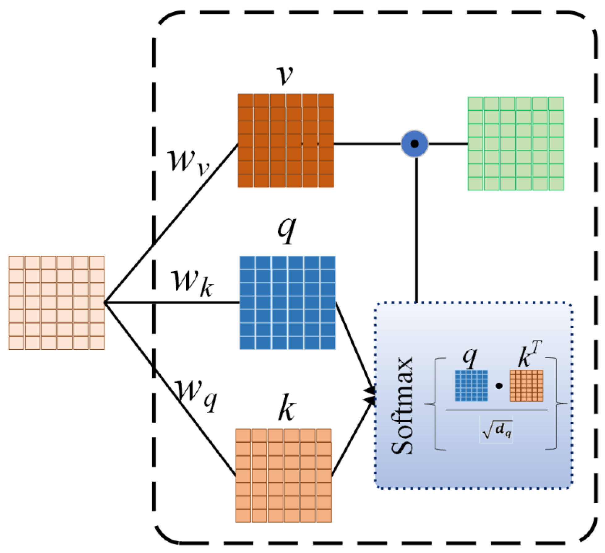
The self-attention mechanism is introduced to enhance the feature representation of input time series by adaptively assigning different weights to the extracted temporal features [38]. This mechanism primarily achieves dynamic weight adjustment and enhances the model’s representational capacity and predictive accuracy through interactions between key matrix (), query matrix (), and value matrix () [39]. The architecture of the self-attention mechanism is illustrated in Figure 4.
Figure 4.
The schematic diagram of the self-attention mechanism structure.
The computation of the self-attention mechanism consists of the following three steps, and the related equations are shown in Equations (11)–(13).
Step 1: Perform three distinct linear transformations on the sequence output of Bi-LSTM to derive keys, values, and query matrixes, i.e., , , and .
Step 2: Compute the relevance score of each element in the sequence by calculating the dot product between and the transpose of the , followed by scaling and SoftMax normalization to obtain attention weights.
Step 3: Calculate the weighted sum of the using attention weights to produce the final self-attention output.
In the equation, is the input sequence; , and are linear transformation weights corresponding to ; , , are query matrix, key matrix, and value matrix, respectively; is the dimensionality of key vectors; represents attention weights; and denotes the attention output.
By incorporating the self-attention mechanism, the model can more accurately focus on key factors with a significant impact on current ship motion dynamics, thereby improving the accuracy and reliability of ship motion prediction.
3. The Model Architecture of SMAPNet
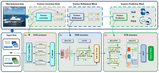
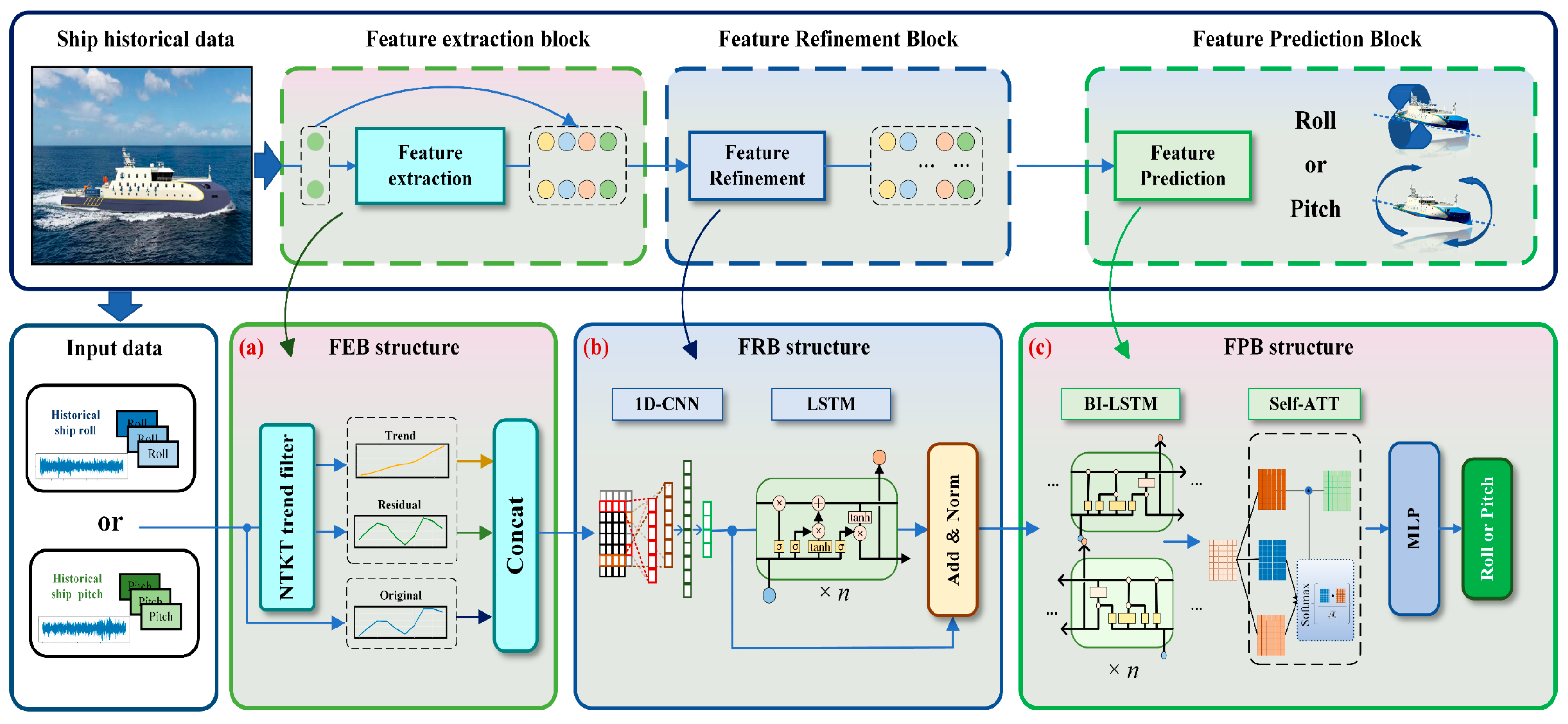
Ocean-going ships are influenced by both ship-specific factors and marine environmental conditions, resulting in complex nonlinear and non-stationary characteristics in ship motion attitude. To improve the adaptability of the prediction model to such time-varying signals, this paper proposes SMAPNet, a hybrid intelligent prediction model integrating the Non-Symmetric Tri-Cube Kernel Trend Filter (NTKTF). The model consists of three functional modules, namely the Feature Extraction Block (FEB), Feature Refinement Block (FRB), and Feature Prediction Block (FPB), as illustrated in Figure 5. First, NTKTF is used in FEB to incrementally decompose the original ship motion attitude sequence into a trend component and a residual component. The trend component reflects the slowly varying tendency of ship motion, while the residual component contains time-varying periodic fluctuations and disturbance-related information caused by wind, waves, and other environmental factors. Then, the original sequence, trend component, and residual component are jointly fed into FRB, where 1DCNN and LSTM are employed to extract local temporal features and long-term dependencies. Finally, FPB integrates Bi-LSTM and a self-attention refinement layer to further process the temporal features and output the predicted ship motion attitude.
Figure 5.
Flowchart of SMAPNet-based ship motion attitude prediction framework.
3.1. Feature Extraction Block—FEB
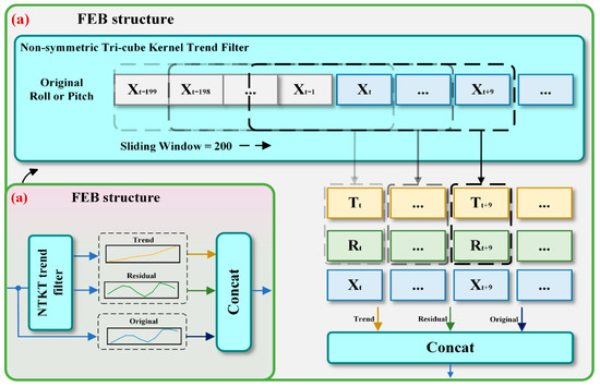
Ocean-going vessels typically have complex and irregular periodicity since their motion and attitude are susceptible to multiple factors such as waves, wind, and tides. Therefore, this paper used NTKTF to design the FEB module, incrementally extracting the trends of ship motion and attitude as well as residual components containing time-varying periodicities and noise caused by multiple factors, and then merging them with original sequences in the feature dimension as input to the FRB module. The structural profile of the FEB module is shown in Figure 6.
Figure 6.
FEB structural analysis diagram, where the value of 200 denotes the NTKTF sliding-window length used for online trend extraction.
3.2. Feature Refinement Block—FRB
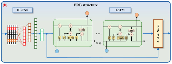
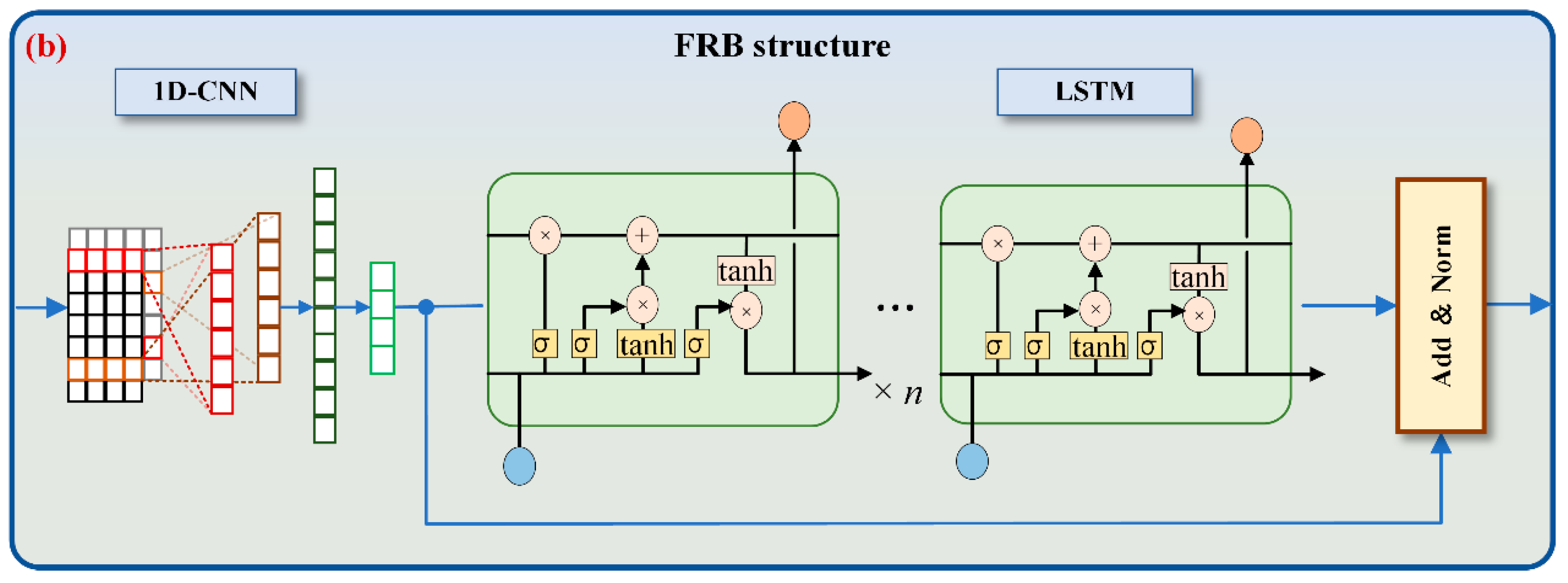
The FRB module is designed to further extract and refine features from the output of the FEB module. As shown in Figure 7, FRB module employs a 1D convolution operation to capture local patterns in the ship motion attitude time series, extracting short-term temporal features while utilizing the LSTM layer to model long-term temporal dependencies within sequences. To address the potential issue of data loss and gradient vanishing in deep networks, the FRB module incorporates residual connections and applies layer normalization techniques to the merged outputs of the LSTM layer and convolutional layer. This architecture effectively integrates local spatial features acquired through convolution with temporal dependencies captured via the LSTM layer, thereby boosting the representational capacity of the model. Note that no pooling layer was applied after 1D convolution, as the ship motion attitude dataset is relatively small compared with image data.
Figure 7.
Schematic diagram of FRB structure.
3.3. Feature Prediction Block—FPB
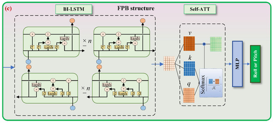
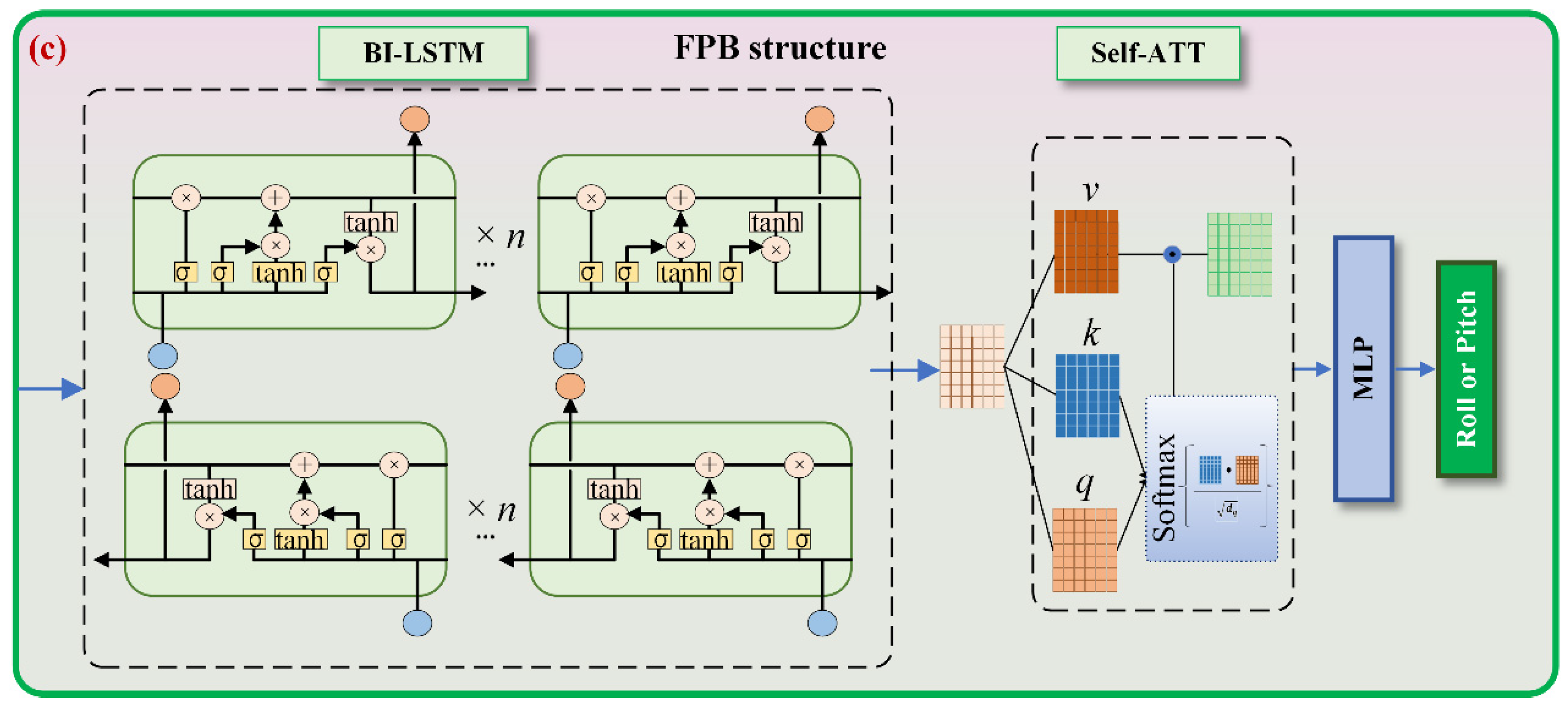
The primary function of the FPB module is to further process the output features of the FRB module and generate accurate predictions of roll or pitch motion. The detailed structure of the FPB is depicted in Figure 8. The module employs Bi-LSTM to incorporate historical and future data, effectively capturing long-term dependencies within the sequence. After temporal modeling by the Bi-LSTM layer, the hidden feature at the final time step is selected as the input for subsequent prediction. This feature is obtained through recurrent state propagation and updating, and can summarize the prediction-related temporal dependencies within the input window. It is then fed into the self-attention refinement layer to further enhance the final recurrent representation before regression.
Figure 8.
Schematic diagram of FPB structure.
4. Experimental Setup
4.1. Data Source and Preprocessing
To assess the forecasting capability of the SMAPNet model for roll and pitch of ocean-going ships, this study analyzed the navigation data gathered during the voyage of the research and training multi-purpose ship XIN HONG ZHUAN from Dalian Port to Shekou Port. The principal dimensions of XIN HONG ZHUAN are outlined in Table 1.
Table 1.
Principal dimensions of XIN HONG ZHUAN.
In this experiment, three levels of standard sea state and four levels of moderate sea state were selected as test conditions. The model’s predictive capability validation and generalization performance evaluation were accomplished through synchronized ship motion data under bimodal sea state conditions. Two datasets of ship motion attitude extracted during the voyage, sampling intervals, and corresponding sea states are listed in Table 2.
Table 2.
Detailed information of the real ship dataset.
Since the selected data segments correspond to short-duration navigation records, the loading and draft conditions are regarded as approximately constant operating conditions in the present prediction task. The raw roll and pitch data collected during the real-ship voyage contained a small number of missing values. Considering the continuous and smooth variation of roll and pitch motions, cubic spline interpolation was adopted to reconstruct short missing intervals while avoiding abrupt discontinuities in the attitude time series. Given that the output of the FEB in the SMAPNet model integrates the original roll or pitch sequence with the trend and residual components, the Min-Max normalization technique was applied in this study to handle the FEB’s output, so as to remove scale inconsistencies, expedite model convergence, and bolster the model’s stability and generalization capacity.
4.2. Data Partitioning and Online Prediction Setup
This paper used the motion attitude of a real ship under sea states of levels three and four to establish an online prediction scenario, with the first 80% of the samples selected as the training set, and the remaining 20% selected as the testing set. A sliding window of size 10 and step size 1 was used to extract sequence features. The trend, residual components, and original sequence output by the FEB module are subjected to Min-Max normalization to eliminate dimensional effects and accelerate model convergence. Prior to the training phase, the training set is pre-decomposed using the FEB module. During the training phase, the two decomposed components were used along with the original sequence to train FRB and FPB modules. In the validation phase, a data stream update mechanism with 1 point per second was employed to simulate an online scenario, and FEB module was used for online incremental decomposition. The experiments were conducted on a computer running Python 3.9.21, with the main software and hardware versions shown in Table 3.
Table 3.
Hardware and software versions.
4.3. Evaluation Metrics
In this paper, the primary assessment criteria of Mean Absolute Error (MAE), Mean Square Error (MSE), and Root Mean Square Error (RMSE) were utilized to evaluate the accuracy of ship motion attitude prediction. MAE is robust to outliers, reflecting the average deviation of fused data while potentially overlooking isolated anomalies. MSE quantifies prediction inaccuracy by squaring discrepancies between predicted and true values. RMSE amplifies squared errors, emphasizing large deviations attributable to sparse outliers. Their combined application effectively reveals both global and granular errors in predicted and actual ship motion attitudes. The formulas for each evaluation metric are presented in Equations (14)–(16).
where is the true value; is the predicted value; is the number of samples; and are the maximum and minimum values of true values, respectively.
4.4. Hyperparameter Settings and Comparative Models
4.4.1. Selection of Sliding Window Size for NTKTF
As shown in Section 2.1, NTKTF requires a sliding window to extract the trend component from historical and current observations. The window size directly affects the balance between trend smoothing and dynamic response. An excessively small window may provide insufficient historical information, causing high-frequency fluctuations to remain in the extracted trend component and leading to under-smoothing. Conversely, an excessively large window may not only increase computational cost, but also cause trend-estimation lag and induce over-smoothing. Therefore, it is crucial to determine an appropriate sliding window size for NTKTF to balance decomposition effectiveness, response delay, and computational cost.
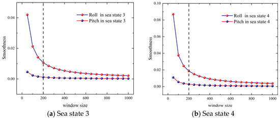
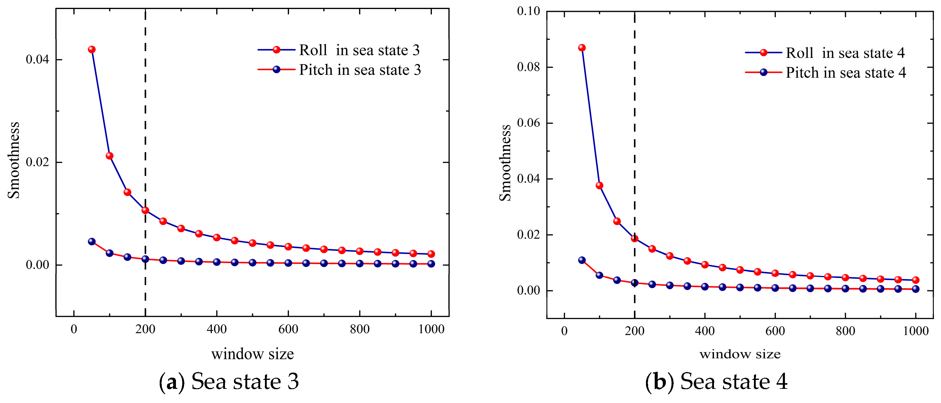
Smoothness is adopted as a core indicator to guide the parameter selection of NTKTF by analyzing its variation with window size. As the window size increases, the smoothness curve gradually approaches a stable region. Therefore, the convergence inflection point is adopted as a practical criterion for NTKTF parameter selection, where the trend component can be sufficiently smoothed while avoiding unnecessarily large window sizes that may increase computational cost and trend-estimation lag. Accordingly, the convergence inflection point of the smoothness curve is adopted to determine an appropriate window size for NTKTF. The formula for calculating smoothness is shown in Equations (17)–(19). To determine the optimal sliding window size, this paper selected a series of window sizes within the range of 50 to 1000, with a step size of 50 to plot the smoothness of the trend component of the ship’s motion attitude under three-level and four-level sea conditions as a function of the sliding window size (as shown in Figure 9), observing the variation of smoothness with the sliding window size.
where is the i-th element in the trend sequence, i is the difference between two adjacent items in the trend sequence, represents the mean value of , and S is the smoothness.
Figure 9.
Smoothness of the trend components of ship motion attitude under different sea states as a function of sliding window size.
As shown in Figure 9, the smoothness of the roll trend component decreases rapidly with the increase in the window size under different sea conditions before the sliding window size reaches 200 in NTKTF. Afterwards, the decrease becomes more gradual, indicating that setting the sliding window to 200 adequately captures the trend of the ship’s roll motion. A further increase in the window size does not significantly improve the smoothing effect and may lead to trend lag, resulting in delayed responses to sudden changes. The smoothness of the pitch trend component also stabilizes gradually after the sliding window reaches 200 under different sea conditions. Therefore, a sliding window size of 200 was selected for NTKTF in this study to enable the filter to fully extract the trend of the ship motion attitude without causing trend lag, while minimizing computational costs.
4.4.2. Hyperparameter Settings for the Network Structure of SMAPNet
The selection of hyperparameters directly affects the feature extraction capability, model complexity, and computational efficiency of the ship motion attitude prediction model. Considering the input sequence length, data scale, model complexity, and computational efficiency, the hyperparameter search ranges in this study were set as follows: kernel_size ∈ [2, 5], kernel_number ∈ [8, 32], hidden_size ∈ [8, 128], and num_layers ∈ [1, 5]. Table 4 lists the optimal network architecture hyperparameters and input/output tensor dimensions for each layer in the SMAPNet prediction model.
Table 4.
Optimal hyperparameters for each module in the SMAPNet model and the corresponding input–output tensor shapes for each layer.
4.4.3. Comparative Models and Training Settings
LSTM [40]: A traditional neural network frequently employed for sequential data prediction to extract long-term dependencies in sequences through three gate mechanisms and cell status.
Bi-LSTMC [24]: Bi-LSTMC combines Bi-LSTM with CNN to create a hybrid deep learning framework, thereby improving the prediction accuracy by leveraging bidirectional temporal feature extraction and temporal-convolutional local feature mining.
ConvLSTM-XGBoost [41]: ConvLSTM-XGBoost enhances the forecasting accuracy of ship motion by integrating spatiotemporal characteristics and dynamic adjustment mechanisms, and combines Convolutional Long Short-Term Memory Networks (ConvLSTM) with Extreme Gradient Boosting (XGBoost) to capture the nonlinear and stochastic nature of ship motions.
ConvLSTMPNet [25]: ConvLSTMPNet is a hybrid deep learning model designed to jointly extract temporal-spatial features and dynamic nonlinear characteristics through a parallel LSTM network and 1DCNN, thereby overcoming the constraints of conventional mechanism-based approaches in intricate maritime settings.
The prediction of ship roll and pitch motions mainly aims to provide predictive information for the ship stabilization system and offer potential support for control strategy adjustment; this paper therefore focused on single-step prediction of ship motion attitudes. Targeting the performance of the SMAPNet forecasting model, the aforementioned forecasting models were selected for comparison with SMAPNet in this study. The optimized parameter configurations of each model are presented in Table 5. The quantity of training iterations is not defined for the ConvLSTMPNet technique, as it utilizes a rolling cross-validation training process.
Table 5.
Main hyperparameter settings for each model.
5. Results and Analysis
In this experiment, two sets of measured motion attitude data from the ocean-going ship XIN HONG ZHUAN under sea state 3 and sea state 4 were employed to conduct prediction analysis of roll and pitch motions. The prediction curves are first used to qualitatively compare the prediction ability of different models. Subsequently, quantitative analysis is conducted using overall evaluation metrics, time-series variations in evaluation metrics, and error distribution plots. The proposed model was compared with various forecasting models for ship roll and pitch under sea state 3, and its robustness was further validated under sea state 4, demonstrating the adaptability of SMAPNet in predicting ship motion attitudes under different marine environments.
5.1. Prediction and Discussion of Ship Motion Attitude Under Sea State 3
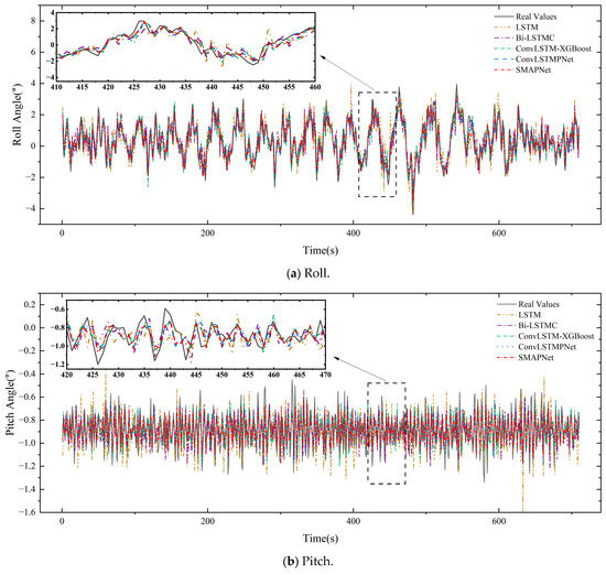
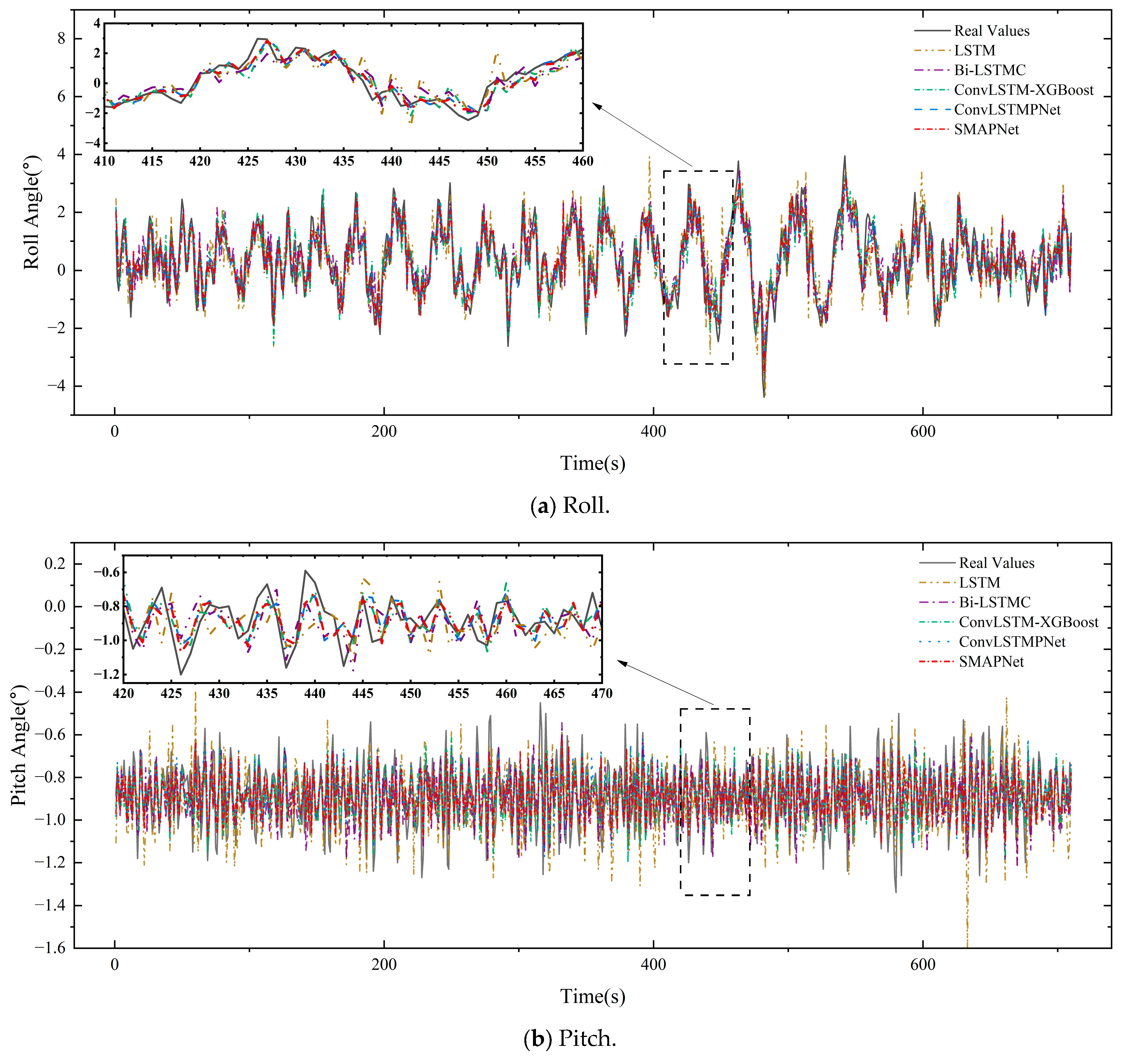
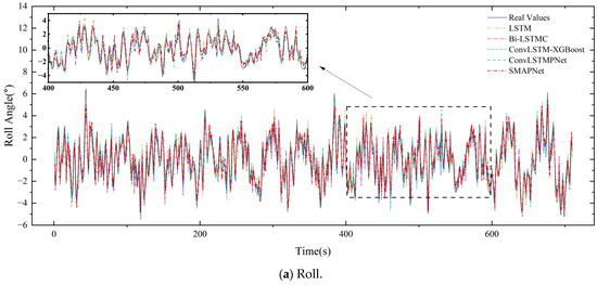
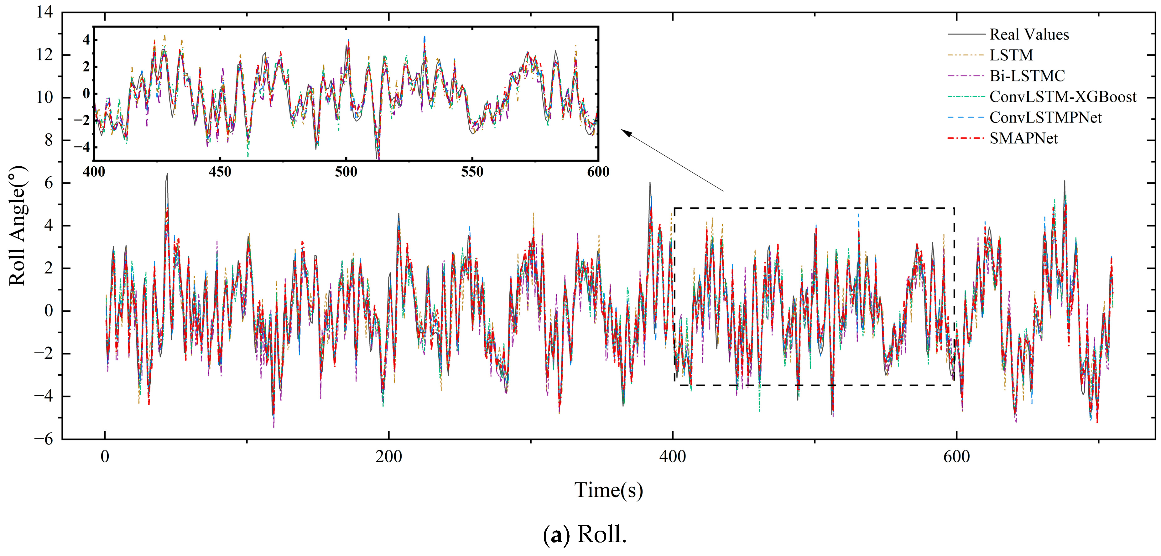
The contrasts between forecast and actual measurements of ship roll and pitch motions by various models and SMAPNet in sea state 3 conditions of the Yellow Sea are depicted in Figure 10. Notably, the ship roll motion demonstrates significant instability without a pronounced long-term trend, marked by frequent oscillations and substantial amplitudes over short intervals. Compared with the roll motion, the pitch motion demonstrates higher oscillation frequencies but smaller amplitudes, with no discernible periodic pattern. Most models show degraded prediction accuracy in peak regions. LSTM, Bi-LSTMC, and ConvLSTM-XGBoost exhibit relatively poor predictive performance in the roll and pitch non-peak regions. Despite the improved accuracy in non-peak regions, SMAPNet shows slightly better agreement with the measured peaks than ConvLSTMPNet, indicating improved overall prediction performance.
Figure 10.
Comparison of roll and pitch predictions of each model in the Yellow Sea under sea state 3.
To further illustrate the performance of the proposed method in predicting ship roll and pitch, its quantitative evaluation indicators are shown in Table 6. Compared with the conventional time series prediction model LSTM, Bi-LSTMC, ConvLSTM-XGBoost, and ConvLSTMPNet models demonstrate moderate improvements in the performance of ship motion prediction, and ConvLSTMPNet outperforms both BI-LSTMC and ConvLSTM-XGBoost. The joint parallel mechanism of convolutional neural networks and Long Short-Term Memory Networks used in ConvLSTMPNet exhibit their effectiveness in extracting non-peak regions from complex dynamic time-varying sequences. The proposed SMAPNet model displays better evaluation metrics than those of ConvLSTMPNet in roll and pitch prediction, with a decrease in MSE, MAE, and RMSE by 10.45%, 5.62%, 5.35%, and 6.96%, 2.76%, 1.1%, respectively. This is because ConvLSTMPNet does not perform feature decoupling on dynamically time-varying ship motion attitude, thereby failing to perform deep learning on the sequences. Additionally, it lacks a feature refinement module similar to the SMAPNet model, resulting in insufficient information extraction capabilities.
Table 6.
Evaluation metrics across various models designed for predicting roll and pitch in the Yellow Sea under sea state 3.
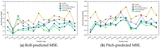
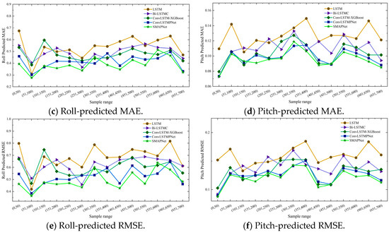
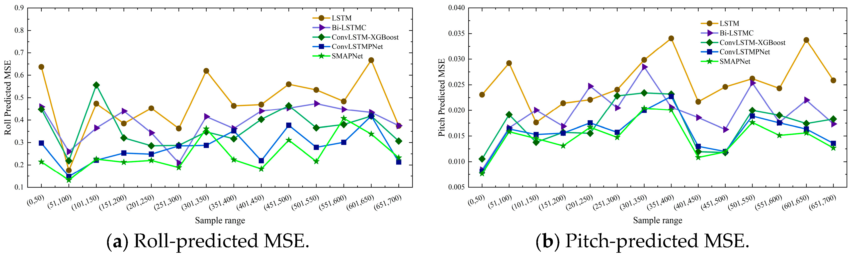
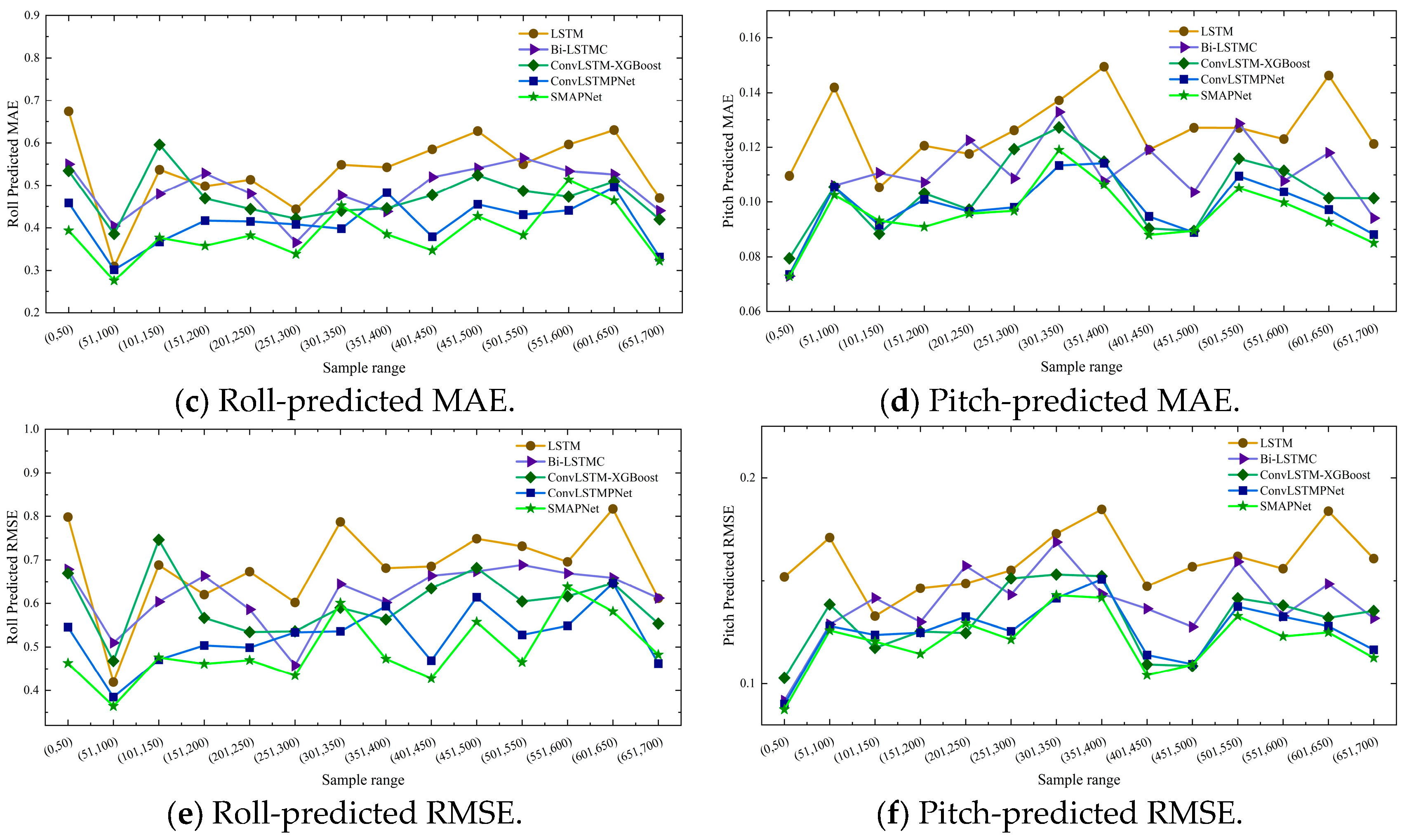
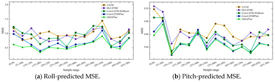
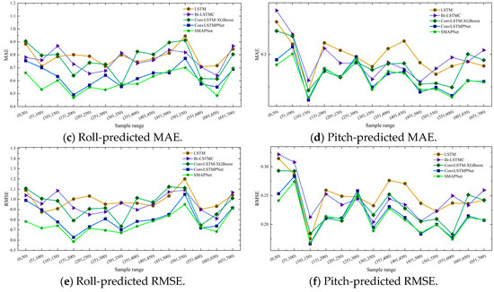
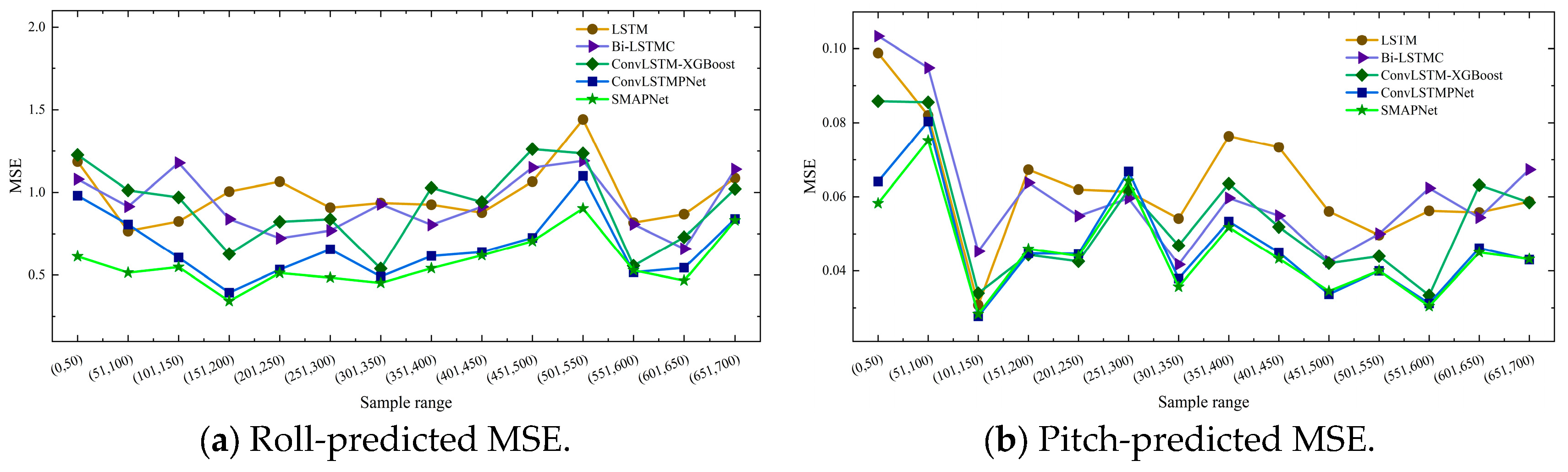
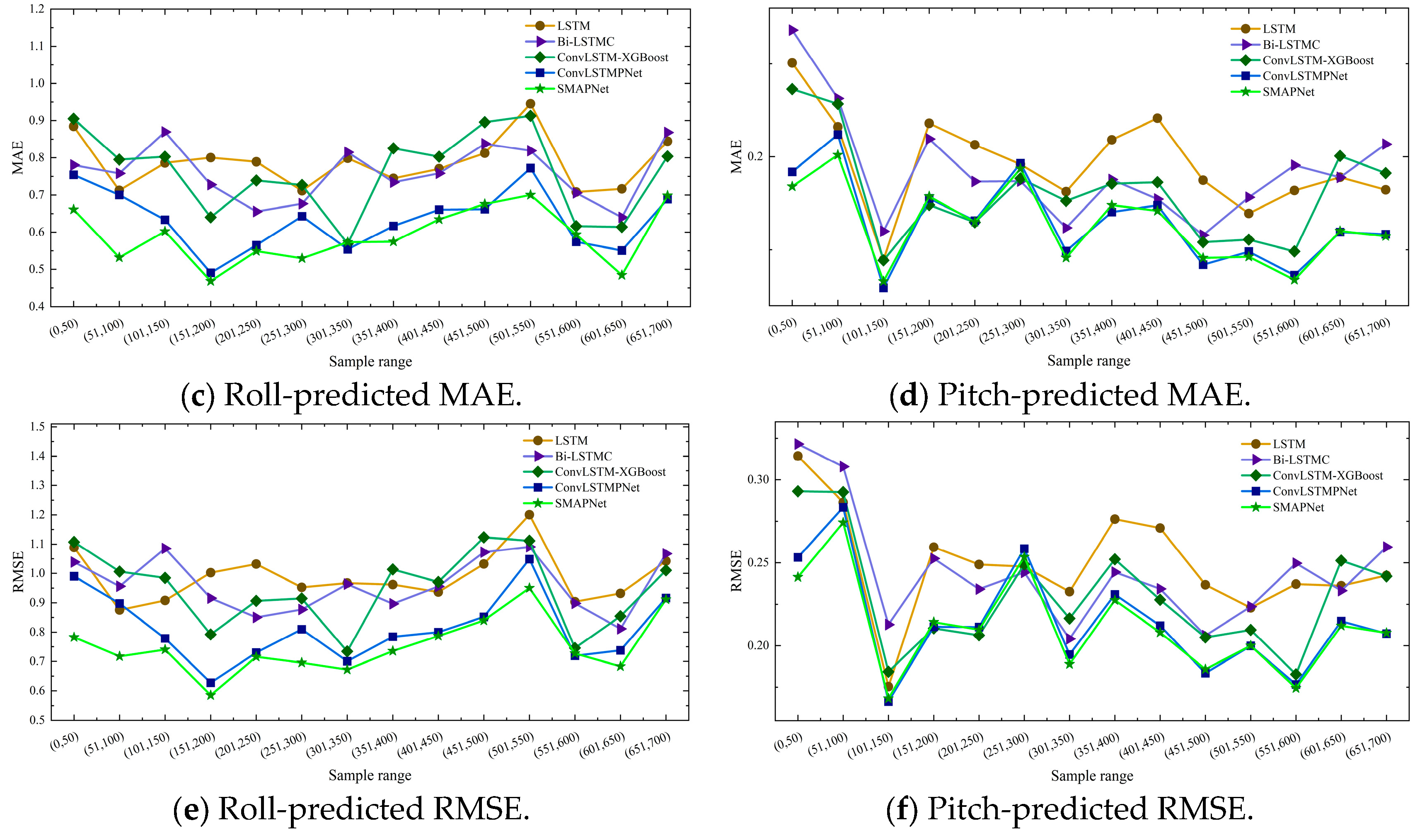
Due to the dynamic time-varying nature of ship motion, a non-overlapping equal-length sliding window of size 50 was employed to better analyze time-varying changes in various evaluation indicators. This window was used to analyze time series changes in performance indicators for the roll and pitch prediction results of different models. Time series changes in various evaluation indicators for roll and pitch predictions of each model under sea state 3 are shown in Figure 11. Notably, metrics of LSTM, BI-LSTM, and ConvLSTM-XGBoost exhibit significant fluctuations and high values, indicating limited dynamic adaptability. SMAPNet and ConvLSTMPNet demonstrate relatively better performance across all evaluation metrics. ConvLSTMPNet performs slightly better than SMAPNet in certain intervals, while SMAPNet outperforms ConvLSTMPNet in overall performance and stability. These results indicate that SMAPNet achieves better overall prediction performance than the benchmark models.
Figure 11.
Time series change diagrams of various evaluation indicators for roll and pitch predictions by each model under sea state 3.
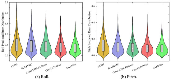
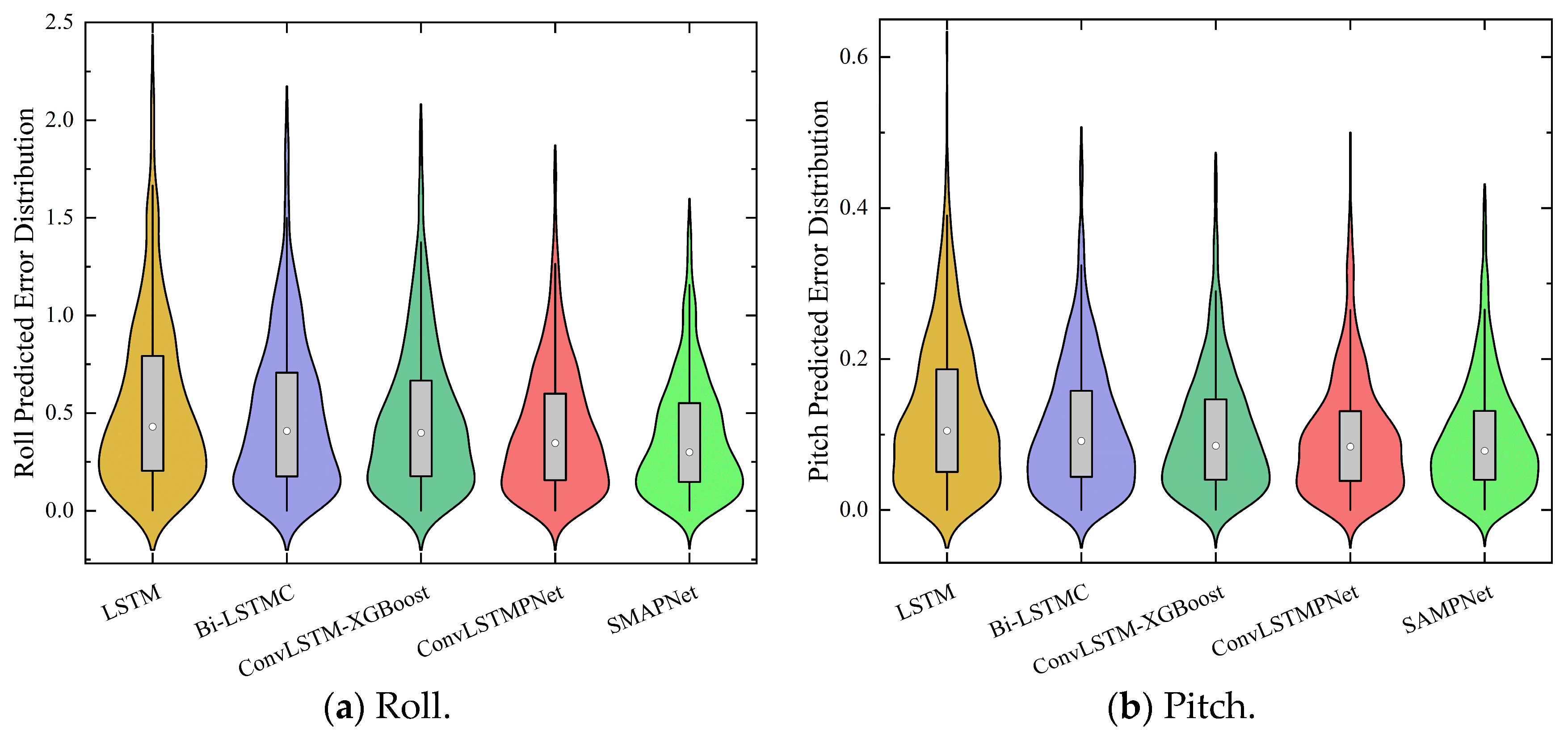
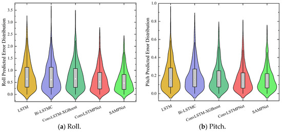
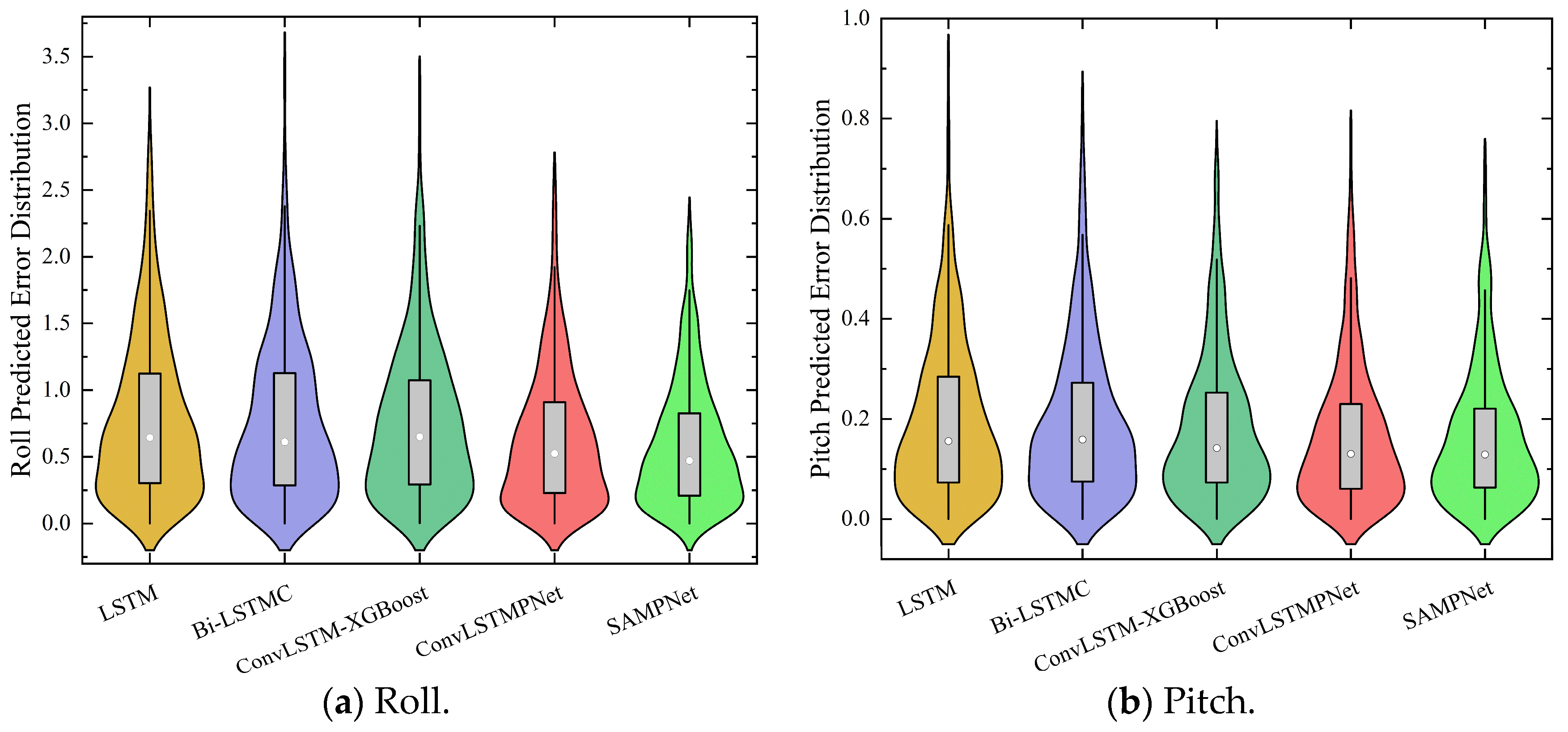
We have obtained the overall error level of the models through evaluation metrics including MSE, MAE, and RMSE, and quantitatively assessed the model performance. However, these metrics did not capture the specific distribution characteristics of the errors. To better characterize the prediction error patterns, error distribution plots of ship motion attitude predictions were presented across different models. By analyzing the magnitude and spatial distribution of errors, the predictive precision of each model can be more accurately evaluated. The error distributions for ship motion attitude predictions are illustrated in Figure 12. From the perspective of error distribution range, SMAPNet exhibits a more concentrated prediction error distribution in roll and pitch motions compared with ConvLSTMPNet, with smaller errors and a tighter distribution. The error distribution ranges of LSTM, BI-LSTM, and ConvLSTM-XGBoost are even broader, indicating less stable prediction results. In terms of median and box structure, SMAPNet exhibits the lowest median value and a compact box structure, indicating favorable central tendency of prediction errors, with most error values concentrated in a lower range. In contrast, other models demonstrate higher median values and wider box structures, suggesting a more dispersed error distribution and unstable prediction performance, the SMAPNet model introduced in this study demonstrates optimal prediction performance across three dimensions—local prediction accuracy, evaluation metrics, and error distribution—enabling more precise ship motion attitude prediction under sea state 3.
Figure 12.
Error distribution in ship motion attitude prediction using each model under sea state 3.
5.2. Prediction and Discussion of Ship Motion Attitude Under Sea State 4
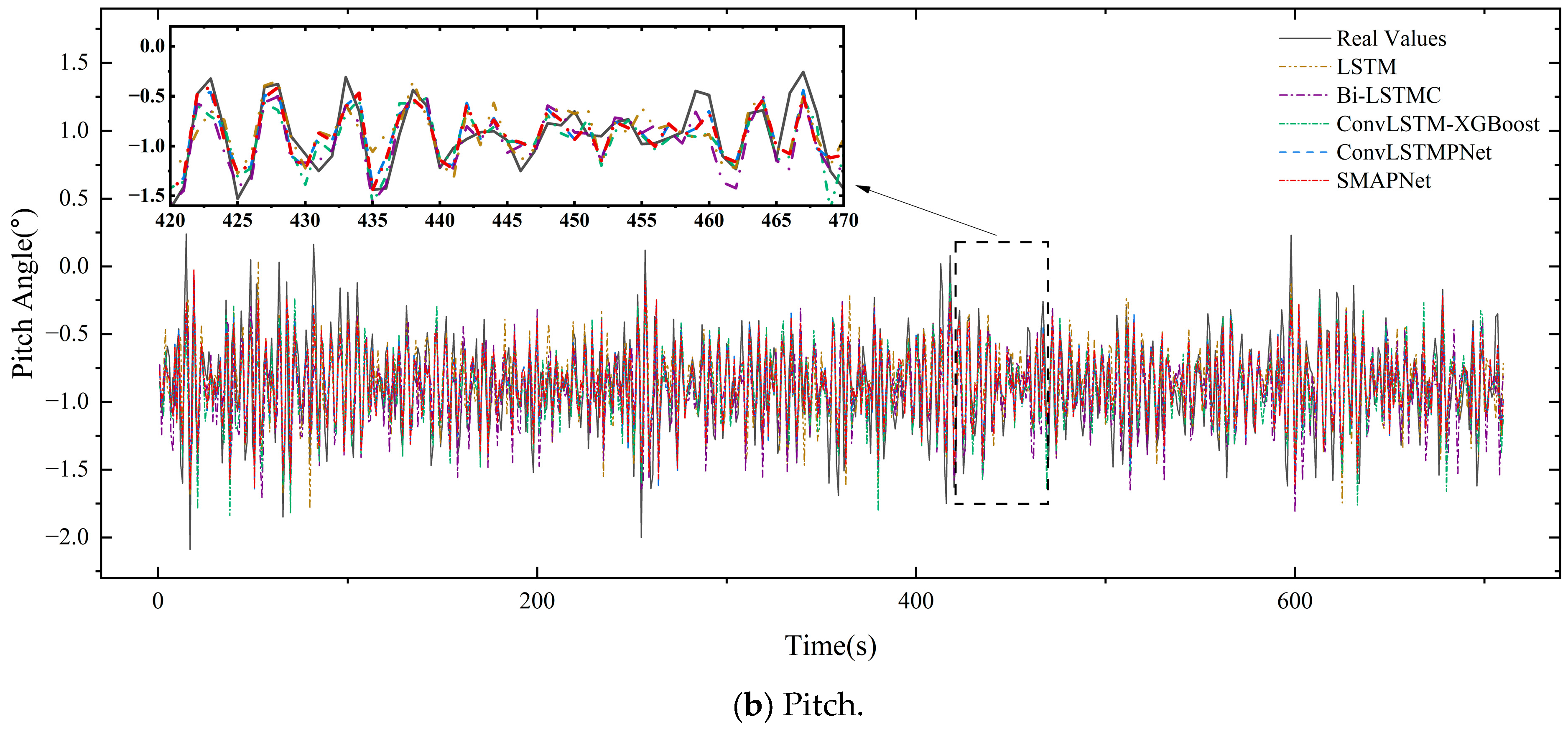
Figure 13 depicts the comparison between forecast and actual measurements of ship roll and pitch motions by each model and SMAPNet in East China Sea under sea state 4 conditions. Compared with the sea state 3 scenario, the ship roll motion under sea state 4 exhibits higher oscillation frequency in the short term, with more pronounced amplitude intensification, an increase of approximately 50% in magnitude and further reduced motion stability. Although no significant changes were observed in the oscillation frequency of the pitch motion, its amplitude demonstrates over 30% augmentation. The overall prediction performance of LSTM, BI-LSTMC, ConvLSTM-XGBoost, and ConvLSTMPNet on ship roll and pitch motions shows significant degradation compared with sea state 3, with particularly pronounced deterioration in the prediction accuracy near motion peaks. In contrast, the SMAPNet model exhibits enhanced prediction accuracy at motion peaks compared with ConvLSTMPNet, demonstrating its accuracy.
Figure 13.
Comparison of roll and pitch predicted by each model in the East China Sea under sea state 4.
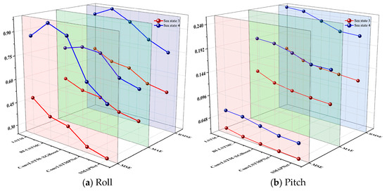
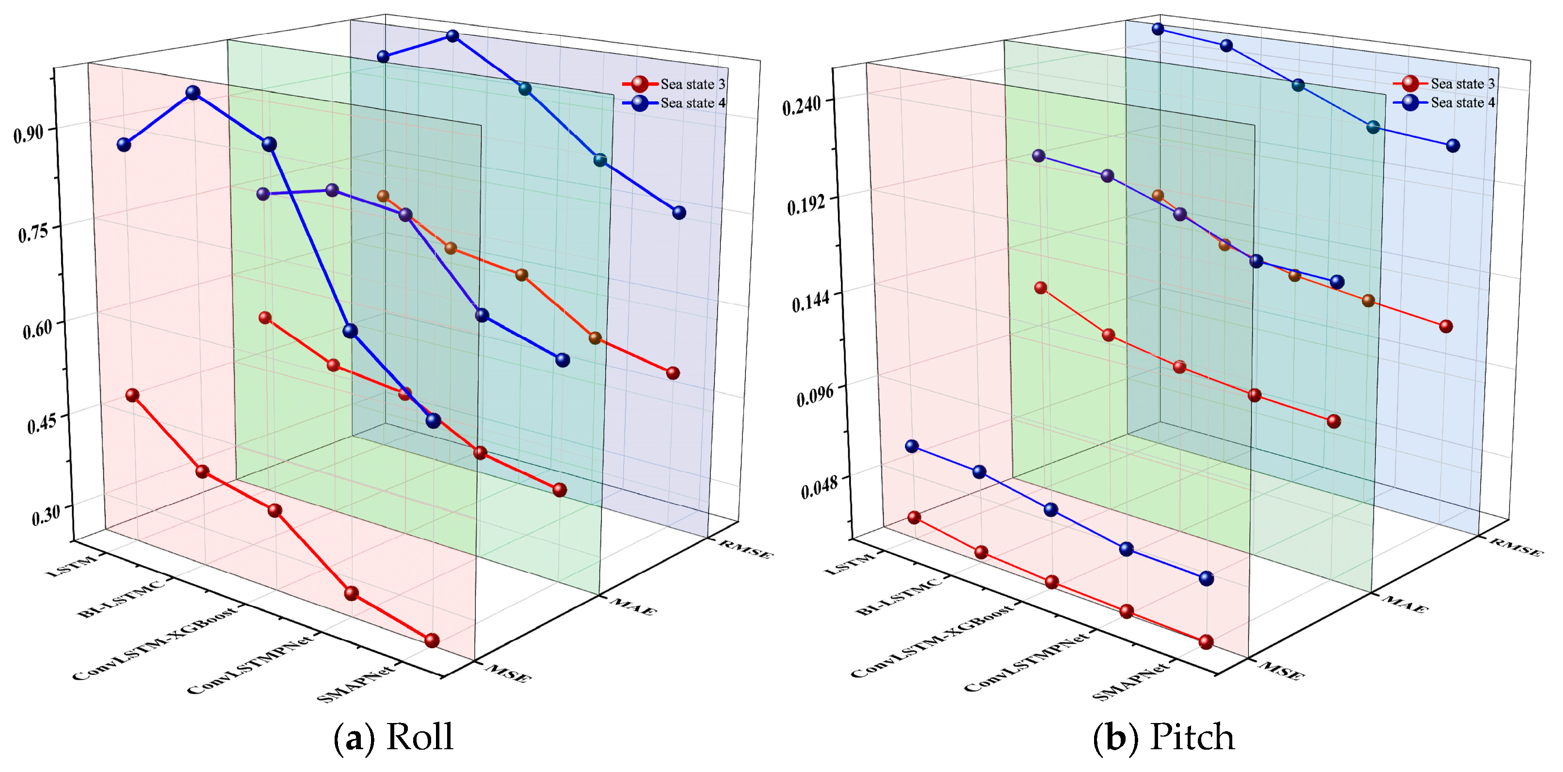
The comparative analysis of quantitative evaluation metrics for the prediction of ship motion attitude across different maritime regions is presented in Table 7 and Table 8. Figure 14 delivers a more vivid visual comparison of evaluation metrics across various models and sea states. Obviously, Bi-LSTMC, ConvLSTM-XGBoost, and ConvLSTMPNet exhibit varying degrees of performance degradation in predictive performance under sea state 4 in the East China Sea, but all outperform LSTM. Among these three models, ConvLSTMPNet demonstrates the lowest performance degradation rate. Specifically, MSE, MAE, and RMSE show an increase of 141.95%, 53.06%, and 55.54% for roll prediction and an increase of 197.47%, 69.08%, and 72.63% for pitch prediction, respectively. Compared with ConvLSTMPNet, our proposed SMAPNet model shows slight decreases in evaluation metrics under higher sea states, and MSE, MAE, and RMSE show a decrease of 14.60%, 6.30%, 7.60% for roll motion and a decrease of 2.77%, 1.10%, 1.43% for pitch motion, respectively, exhibiting a satisfactory accuracy. It is worth noting that the RMSE values appear higher than the other evaluation metrics, mainly because the squared-error calculation makes RMSE more sensitive to local peak deviations than MAE
Table 7.
Comparative analysis of evaluation metrics for roll prediction across models in different maritime regions.
Table 8.
Comparative analysis of evaluation metrics for pitch prediction across models in different maritime regions.
Figure 14.
Comparison of evaluation metrics of models for ship motion attitude prediction under different sea states.
Time-series changes in various evaluation metrics for roll and pitch predictions under sea state 4 conditions are shown in Figure 15. Under sea state 4 conditions, LSTM and BI-LSTMC have limited capabilities in understanding complex time-series characteristics and nonlinear relationships of ship motion, resulting in relatively high metric values and difficulty in effectively capturing patterns of the motion. ConvLSTM-XGBoost shows relatively unstable performance and weak adaptability to changes in sea conditions despite its competitive accuracy compared with Bi-LSTMC in certain regions. Despite a phased improvement in performance compared with the aforementioned methods, the prediction accuracy and overall stability of ConvLSTMPNet are inferior to SMAPNet. Therefore, SMAPNet exhibits stronger adaptability to changes in sea conditions compared with other models.
Figure 15.
Time series change diagrams of various evaluation indicators for roll and pitch predictions by each model under sea state 4.
Figure 16 shows the error distribution of each model in predicting ship motion attitude under sea state 4. Notably, Bi-LSTMC, ConvLSTM-XGBoost, and ConvLSTMPNet have wider error distribution ranges and boxplot structures, with more dispersed error distributions and relatively poor model stability. Despite a certain degree of concentration in its box structure, ConvLSTMPNet exhibits a wider error distribution range compared with SMAPNet and a slightly higher median. In summary, SMAPNet provides better peak-region fitting and achieves lower errors in the adopted evaluation metrics, and demonstrates favorable error convergence characteristics, with smaller and more stable prediction errors. Therefore, SMAPNet can maintain high prediction accuracy in both typical Yellow Sea conditions and more complex East China Sea environments.
Figure 16.
Error distribution in ship motion attitude prediction using each model under sea state 4.
5.3. Extended Prediction Horizon Analysis
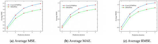
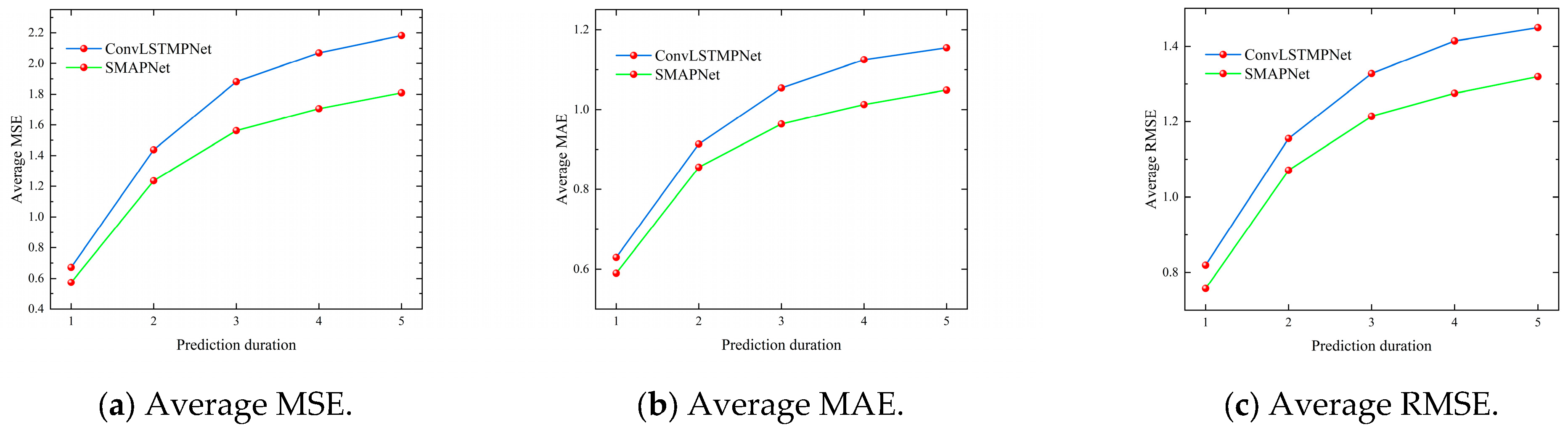
To investigate the impact of increasing prediction time on prediction accuracy, a predictive analysis of roll motion was conducted under the most dynamically time-varying conditions of sea state 4. Regarding the comparison between SMAPNet and ConvLSTMPNet, the number of model outputs was adjusted and the prediction horizon was extended to 2 to 5 s. MSE, MAE, and RMSE were selected as evaluation metrics for prediction accuracy. Figure 17 shows the curve targeting the average evaluation metrics of prediction results in the two models as a function of prediction time. As the prediction time increases, the prediction accuracy gradually decreases. However, SMAPNet achieves better prediction results than ConvLSTMPNet.
Figure 17.
Curves of average evaluation indicators over time.
5.4. Comparison of Training and Inference Time for Each Model
The SMAPNet model proposed in this paper integrates multiple functional modules. On this basis, a comparative analysis of training and prediction times was conducted to comprehensively evaluate the computational efficiency of the model, quantified from two dimensions: the average time per epoch during the training phase and the average time per time step during the prediction phase. Statistical results are shown in Table 9. The LSTM model does not integrate other algorithms, showing the shortest training and prediction time. The ConvLSTM-XGBoost model integrates deep learning and ensemble learning, and combines both neural networks and tree models, suggesting the longest training and prediction time. SMAPNet proposed in this paper pre-calls the FEB module prior to the starting of the training phase and performs the training based on its decomposed sequence, without the need to repeatedly call the module during the actual training process. The average computation time per epoch for FRB and FPB modules of SMAPNet was slightly higher than that of Bi-LSTMC and ConvLSTMPNet. During the prediction phase, all modules of SMAPNet were invoked. The average prediction time per step remains within an acceptable range despite being approximately 0.01 ms higher than that of Bi-LSTMC and ConvLSTMPNet.
Table 9.
Training and prediction time for different models.
5.5. Comprehensive Discussion of Comparative Results
Based on the above results, the comparative performance of SMAPNet can be further discussed from the perspectives of feature extraction capability, robustness, and optimization efficiency. In terms of feature extraction, LSTM mainly relies on recurrent temporal modeling, while Bi-LSTMC introduces convolutional structures to capture local temporal patterns and bidirectional temporal dependencies. ConvLSTM-XGBoost combines convolutional recurrent feature extraction with ensemble learning to enhance nonlinear fitting capability. ConvLSTMPNet further adopts a parallel CNN-LSTM structure to jointly extract local and temporal features. In comparison, SMAPNet integrates NTKTF-based incremental decomposition, 1DCNN-based local feature extraction, LSTM/Bi-LSTM-based temporal modeling, and self-attention-based feature refinement. Therefore, the original sequence, trend component, and residual component of ship motion attitude can be jointly utilized for multi-level feature learning.
In terms of robustness, the prediction results under sea states 3 and 4 show that SMAPNet maintains lower prediction errors and more concentrated error distributions than the comparative models. This indicates that the decomposition-refinement-prediction architecture improves the adaptability of the model to nonlinear and non-stationary ship motion attitude signals.
In terms of optimization efficiency, LSTM has the lowest computational cost due to its simple structure, while ConvLSTM-XGBoost requires a longer training and inference time because it combines deep learning with ensemble learning. Although SMAPNet integrates multiple functional modules, its average prediction time per step remains within an acceptable range. Therefore, SMAPNet achieves a practical balance among prediction accuracy, robustness, and computational cost in short-term online prediction of ship motion attitude.
5.6. Ablation Experiments with SMAPNet
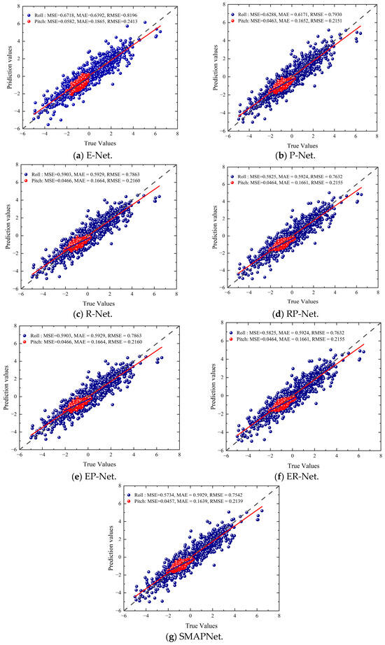
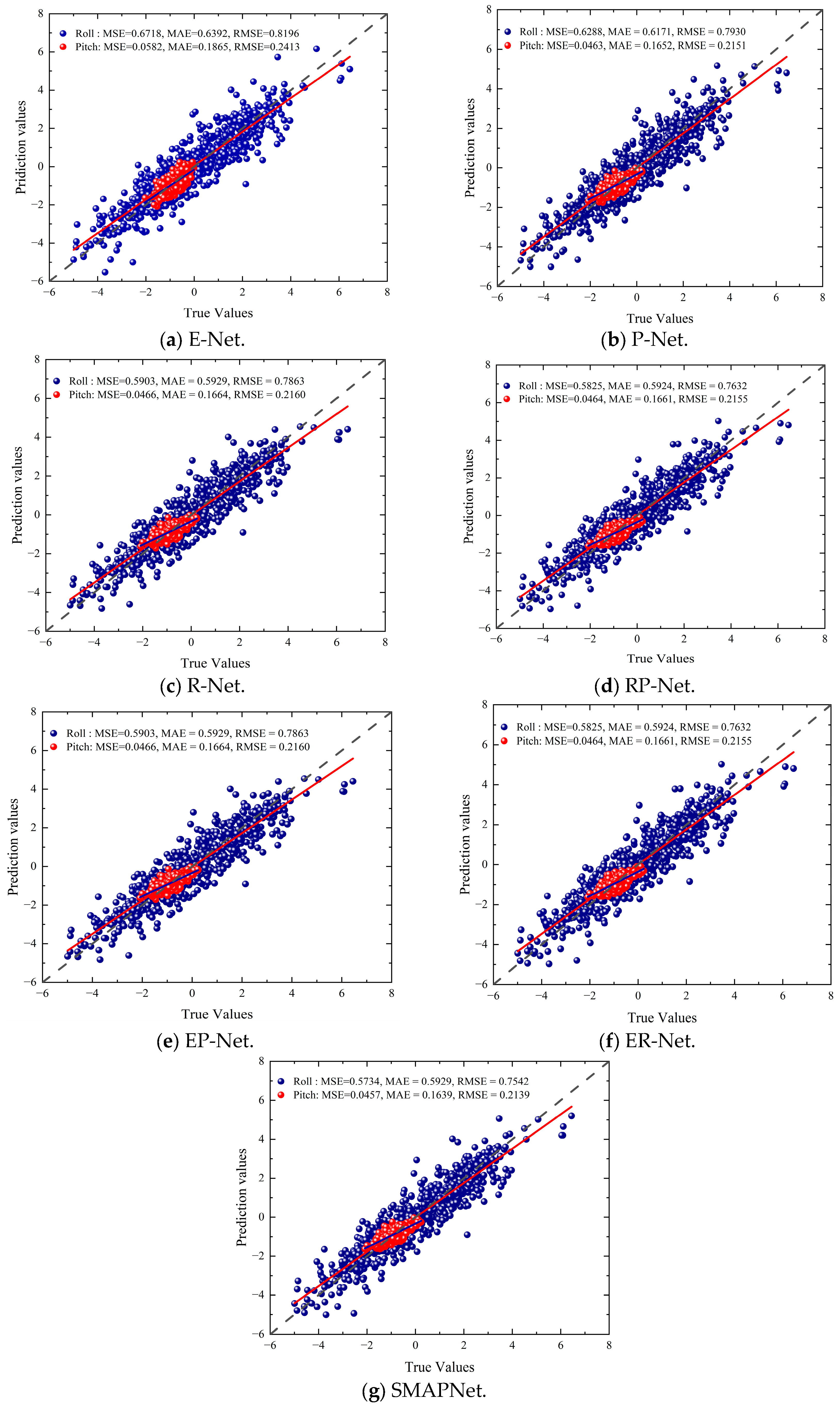
To systematically analyze the efficacy of each module in the SMAPNet model, a series of ablation experiments with ship motion and attitude data under sea state 4 (characterized by time-varying dynamics) was designed to quantitatively evaluate the impact of individual modules on holistic performance by isolating or ablating key components. This approach elucidates the synergistic mechanisms of module interactions to enhance model performance. The standalone implementations of FEB, FRB, and FPB correspond to E-Net, R-Net, and P-Net in ablation studies. In contrast, the module removal configurations correspond to RP-Net (FEB ablated), EP-Net (FRB ablated) and ER-Net (FPB ablated). Analytical results derived from Table 10 are shown as follows. Figure 18 presents a scatter plot of predicted and actual values from various model variants.
Table 10.
Evaluation metrics of different model variants in sea state 4.
Figure 18.
Scatter plot of forecast and actual measurements from various model configurations.
Table 10 and Figure 18 illustrate that the SMAPNet shows the closest overall agreement with the measured values among the tested variants, and the lowest dispersion. E-Net performs best as a standalone model, which is primarily attributed to the efficient decomposition of NTKTF on the ship motion attitude into trend components containing potential trends and residual components containing time-varying periodicities and noise, thereby laying a critical foundation for predictive modeling.
In roll and pitch motion prediction, ER-Net yields lower MSE, MAE, and RMSE than EP-Net, suggesting that the FRB-related structure is more effective in extracting local detailed features in this setting. RP-Net outperforms P-Net and R-Net, and also achieves lower errors than ConvLSTMPNet, the best-performing baseline model in this study. These results indicate that the combined FRB-FPB structure contributes to feature refinement and improves the overall prediction performance.
SMAPNet incorporates FPB into the ER-Net model and reduced the values of various evaluation indicators for roll and pitch predictions, demonstrating that the FPB module can effectively integrate global information extraction with local feature refinement. Bi-LSTM and self-attention mechanisms within the module enable comprehensive assimilation of preceding module outputs while enhancing attention weights allocation to critical features, mitigating the impact of redundant signals and interference noise during the final prediction process.
The above discussion demonstrates that the SMAPNet model design can effectively incorporate the complementary characteristics of three modules, and process ship motion attitude through multi-dimensional approaches, thereby contributing to the overall predictive performance of the model.
6. Conclusions
In this paper, a Ship Motion Attitude Prediction Network (SMAPNet) leveraging Non-Symmetric Tri-Cube Kernel Trend Filter (NTKTF) was proposed to attain short-term forecasting of roll and pitch motions for ocean-going ships through the fusion of time-series decomposition, deep feature extraction, and dynamic attention mechanisms. SMAPNet performed multi-level feature mining of ship motion attitude time-series data through the collaborative design of three modules: the Feature Extraction Block (FEB), Feature Refinement Block (FRB), and Feature Prediction Block (FPB). FEB effectively separated trend and residual components using NTKTF; FRB extracted key features from both local details and global temporal dependencies by integrating 1DCNN with LSTM networks; FPB dynamically allocated feature weights and captured complex nonlinear relationships via Bi-LSTM and self-attention mechanisms. According to the experimental results, SMAPNet reduced the MSE of roll and pitch by 10.45% and 6.96%, respectively, under sea state 3 conditions compared with the optimal reference model. Additionally, SMAPNet reduced the MSE of roll and pitch by 14.60% and 2.77%, respectively, under the relatively harsh sea state 4 conditions, indicating relatively better stability among the tested models. The ablation experiment further validated the synergistic impact of each module. The removal of individual modules generally leads to increased prediction errors, indicating the contribution of each component.
Despite the advantage of SMAPNet in handling stronger non-stationary fluctuations through the NTKTF-based separation of trend and residual components, its performance under sea states higher than 4 has not been directly validated in this study. Therefore, future work will incorporate measured data from higher sea states for further experimental validation.
Author Contributions
Conceptualization, Z.L. (Zhibo Lei) and H.G.; methodology, Z.L. (Zhibo Lei) and H.G.; software, Z.L. (Zhibo Lei); validation, Z.L. (Zhibo Lei), Y.L., Z.L. (Zonghan Li), H.G. and F.S.; formal analysis, Z.L. (Zhibo Lei); investigation, Z.L. (Zhibo Lei), Y.L., H.G., Z.L. (Zonghan Li) and F.S.; resources, H.G.; data curation, H.G.; writing—original draft preparation, Z.L. (Zhibo Lei); writing—review and editing, Z.L. (Zhibo Lei) and H.G.; visualization, Z.L. (Zhibo Lei), Y.L. and Z.L. (Zonghan Li); supervision, H.G.; project administration, H.G.; funding acquisition, H.G. All authors have read and agreed to the published version of the manuscript.
Funding
This research received no external funding.
Data Availability Statement
Dataset available upon request from the authors.
Conflicts of Interest
The authors declare no conflicts of interest.
Nomenclature
| SMAPNet | Ship Motion Attitude Prediction Network |
| NTKTF | Non-Symmetric Tri-Cube Kernel Trend Filter |
| FEB | Feature Extraction Block |
| FRB | Feature Refinement Block |
| FPB | Feature Prediction Block |
| CNN | Convolutional Neural Network |
| RNN | Recurrent Neural Network |
| LSTM | Long Short-Term Memory |
| Bi-LSTM | Bidirectional Long Short-Term Memory |
| EMD | Empirical Mode Decomposition |
| VMD | Variational Mode Decomposition |
| TVF-EMD | Time-varying Filter-based Empirical Mode Decomposition |
| GRU | Gated Recurrent Unit |
| SVR | Support Vector Regression |
| MAE | Mean Absolute Error |
| MSE | Mean Square Error |
| RMSE | Root Mean Square Error |
| DOF | Degrees of Freedom |
| Observation at time t | |
| Observation within the sliding window | |
| Sliding window size | |
| Relative position parameter in the sliding window | |
| Weight of the i-th observation in NTKTF | |
| Trend component at time t | |
| Residual component at time t | |
| Query matrix | |
| Key matrix | |
| Value matrix | |
| Dimensionality of key vectors | |
| True value | |
| Predicted value | |
| Number of samples | |
| Smoothness |
References
- Zhou, B.; Qi, X.; Zhang, J.; Zhang, H. Effect of 6-DOF Oscillation of Ship Target on SAR Imaging. Remote Sens. 2021, 13, 1821. [Google Scholar] [CrossRef] [Scilit]
- Gao, N.; Hu, A.; Hou, L.; Chang, X. Real-time ship motion prediction based on adaptive wavelet transform and dynamic neural network. Ocean Eng. 2023, 280, 114466. [Google Scholar] [CrossRef] [Scilit]
- Xu, S.; Tan, W.; Sun, L. Modeling Shared Control System Between Human Pilot and Autopilot for a Carrier-Based Aircraft Landing Task. IEEE Trans. Hum.-Mach. Syst. 2025, 55, 102–111. [Google Scholar] [CrossRef] [Scilit]
- Zhang, L.; Feng, X.; Wang, L.; Gong, B.; Ai, J. A hybrid ship-motion prediction model based on CNN–MRNN and IADPSO. Ocean Eng. 2024, 299, 117428. [Google Scholar] [CrossRef] [Scilit]
- Trang, N.T.H.; Mitsuyuki, T.; Hirakawa, Y.; Sadakata, K.; Nakamura, Y. Experimental and Numerical Study on the Seakeeping Performance of a Wind-Powered Generation Ship Considering Boom Configurations. J. Mar. Sci. Eng. 2025, 13, 412. [Google Scholar] [CrossRef] [Scilit]
- Wang, Z.; Yang, G.; Li, B.; Xu, Y.; Yuan, C.; Xu, R. Ship pose prediction through an integrated empirical mode decomposition and deep learning method. Ships Offshore Struct. 2025, 1–21. [Google Scholar] [CrossRef] [Scilit]
- Zhao, J.; Zhao, Y. Very short-term forecasting of ship multidimensional motion using two coupled models based on deep operator networks. Ocean Eng. 2025, 317, 120044. [Google Scholar] [CrossRef] [Scilit]
- Jiang, H.; Duan, S.; Huang, L.; Han, Y.; Yang, H.; Ma, Q. Scale effects in AR model real-time ship motion prediction. Ocean Eng. 2020, 203, 107202. [Google Scholar] [CrossRef] [Scilit]
- Zhang, B.; Wang, S.; Ji, S. A deep learning combined prediction model for prediction of ship motion attitude in real conditions. Ships Offshore Struct. 2024, 19, 1868–1883. [Google Scholar] [CrossRef] [Scilit]
- Nielsen, U.D.; Brodtkorb, A.H.; Jensen, J.J. Response predictions using the observed autocorrelation function. Mar. Struct. 2018, 58, 31–52. [Google Scholar] [CrossRef] [Scilit]
- Wang, W.-C.; Chau, K.-W.; Xu, D.-M.; Chen, X.-Y. Improving Forecasting Accuracy of Annual Runoff Time Series Using ARIMA Based on EEMD Decomposition. Water Resour. Manag. 2015, 29, 2655–2675. [Google Scholar] [CrossRef] [Scilit]
- Pena-Sanchez, Y.; Merigaud, A.; Ringwood, J.V. Short-Term Forecasting of Sea Surface Elevation for Wave Energy Applications: The Autoregressive Model Revisited. IEEE J. Ocean. Eng. 2020, 45, 462–471. [Google Scholar] [CrossRef] [Scilit]
- Zheng, K.; Chen, Y.; Jiang, Y.; Qiao, S. A SVM based ship collision risk assessment algorithm. Ocean Eng. 2020, 202, 107062. [Google Scholar] [CrossRef] [Scilit]
- Hoang, A.T.; Bui, T.A.E.; Nguyen, X.P.; Bui, V.H.; Nguyen, Q.C.; Truong, T.H.; Chung, N. Explainable machine learning-based prediction of fuel consumption in ship main engines using operational data. Brodogradnja 2025, 76, 76405. [Google Scholar] [CrossRef] [Scilit]
- Popoola, S.I.; Misra, S.; Atayero, A.A. Outdoor Path Loss Predictions Based on Extreme Learning Machine. Wirel. Pers. Commun. 2017, 99, 441–460. [Google Scholar] [CrossRef] [Scilit]
- Yin, Y.-M.; Cui, H.-Y.; Hong, M.; Zhao, D.-Y. Prediction of the vertical vibration of ship hull based on grey relational analysis and SVM method. J. Mar. Sci. Technol. 2014, 20, 467–474. [Google Scholar] [CrossRef] [Scilit]
- Chen, C.; Ruiz, M.T.; Delefortrie, G.; Mei, T.; Vantorre, M.; Lataire, E. Parameter estimation for a ship’s roll response model in shallow water using an intelligent machine learning method. Ocean Eng. 2019, 191, 106479. [Google Scholar] [CrossRef] [Scilit]
- Liong, C.T.; Chua, K.H. Data assimilation for deterministic prediction of vessel motion in real-time. Ocean Eng. 2022, 244, 110356. [Google Scholar] [CrossRef] [Scilit]
- Ozsari, I. Predicting main engine power and emissions for container, cargo, and tanker ships with artificial neural network analysis. Brodogradnja 2023, 74, 77–94. [Google Scholar] [CrossRef] [Scilit]
- Chen, Z.; Liu, X.; Ji, X.; Gui, H. Real-Time Prediction of Multi-Degree-of-Freedom Ship Motion and Resting Periods Using LSTM Networks. J. Mar. Sci. Eng. 2024, 12, 1591. [Google Scholar] [CrossRef] [Scilit]
- Tang, H.; Zhu, R.; Wan, Q.; Ren, D. Short-term prediction of trimaran load based on data driven technology. Brodogradnja 2025, 76, 76101. [Google Scholar] [CrossRef] [Scilit]
- Yuan, P.; Zhao, W.; Zhao, Y. Intelligent prediction algorithm of ship roll and pitch motion based on SSA- optimized BiLSTM network. Ocean Eng. 2025, 320, 120331. [Google Scholar] [CrossRef] [Scilit]
- Ribeiro, M.H.D.M.; dos Santos Coelho, L. Ensemble approach based on bagging, boosting and stacking for short-term prediction in agribusiness time series. Appl. Soft Comput. 2020, 86, 105837. [Google Scholar] [CrossRef] [Scilit]
- Wang, Y.; Wang, H.; Zhou, B.; Fu, H. Multi-dimensional prediction method based on Bi-LSTMC for ship roll. Ocean Eng. 2021, 242, 110106. [Google Scholar] [CrossRef] [Scilit]
- Zhang, D.; Zhou, X.; Wang, Z.-H.; Peng, Y.; Xie, S.-R. A data driven method for multi-step prediction of ship roll motion in high sea states. Ocean Eng. 2023, 276, 114230. [Google Scholar] [CrossRef] [Scilit]
- Li, P.; Wang, Q.; Chen, N.; Tu, Y.; Lin, X.; Chen, Y. Multi-dimensional ship motion attitude combination prediction based on the SSA-BiGRU-Attention model. Measurement 2025, 253, 117484. [Google Scholar] [CrossRef] [Scilit]
- Fan, G.; Yu, P.; Wang, Q.; Dong, Y. Short-term motion prediction of a semi-submersible by combining LSTM neural network and different signal decomposition methods. Ocean Eng. 2023, 267, 113266. [Google Scholar] [CrossRef] [Scilit]
- Geng, X.; Li, Y.; Sun, Q. A Novel Short-Term Ship Motion Prediction Algorithm Based on EMD and Adaptive PSO–LSTM with the Sliding Window Approach. J. Mar. Sci. Eng. 2023, 11, 466. [Google Scholar] [CrossRef] [Scilit]
- Zhang, Q.; Li, J.-B.; He, A.; Hu, X. Application of Non-Stationary Ship Roll Motion Prediction and Compensation Control Based on VMD-GRU-EC. In Proceedings of the 2024 IEEE 18th International Conference on Control & Automation (ICCA), Reykjavík, Iceland, 18–21 June 2024; pp. 347–352. [Google Scholar]
- Xu, D.; Yin, J. An enhanced hybrid scheme for ship roll prediction using support vector regression and TVF-EMD. Ocean Eng. 2024, 307, 117951. [Google Scholar] [CrossRef] [Scilit]
- Cai, X.; Li, D. M-EDEM: A MNN-based Empirical Decomposition Ensemble Method for improved time series forecasting. Knowl.-Based Syst. 2024, 283, 111157. [Google Scholar] [CrossRef] [Scilit]
- Mishra, A.; Sriharsha, R.; Zhong, S. OnlineSTL: Scaling time series decomposition by 100x. In Proceedings of the VLDB Endowment; ACM: New York, NY, USA, 2022; Volume 15, pp. 1417–1425. [Google Scholar] [CrossRef] [Scilit]
- Yang, S.; Deng, Z.; Li, X.; Zheng, C.; Xi, L.; Zhuang, J.; Zhang, Z.; Zhang, Z. A novel hybrid model based on STL decomposition and one-dimensional convolutional neural networks with positional encoding for significant wave height forecast. Renew. Energy 2021, 173, 531–543. [Google Scholar] [CrossRef] [Scilit]
- Ren, S.; He, K.; Girshick, R.; Sun, J. Faster R-CNN: Towards Real-Time Object Detection with Region Proposal Networks. IEEE Trans. Pattern Anal. Mach. Intell. 2017, 39, 1137–1149. [Google Scholar] [CrossRef] [Scilit] [PubMed]
- Zhao, G.; Liu, G.; Fang, L.; Tu, B.; Ghamisi, P. Multiple convolutional layers fusion framework for hyperspectral image classification. Neurocomputing 2019, 339, 149–160. [Google Scholar] [CrossRef] [Scilit]
- Shi, H.; Miao, K.; Ren, X. Short-term load forecasting based on CNN-BiLSTM with Bayesian optimization and attention mechanism. Concurr. Comput. Pract. Exp. 2021, 35, e6676. [Google Scholar] [CrossRef] [Scilit]
- Meng, L.; Gan, H.; Liu, H.; Lu, D. Deep learning-based research on fault warning for marine dual fuel engines. Brodogradnja 2025, 76, 76303. [Google Scholar] [CrossRef] [Scilit]
- Li, X.; Yuan, A.; Lu, X. Vision-to-Language Tasks Based on Attributes and Attention Mechanism. IEEE Trans. Cybern. 2021, 51, 913–926. [Google Scholar] [CrossRef] [Scilit]
- Wang, N.; Kong, X.; Ren, B.; Hao, L.; Han, B. SeaBil: Self-attention-weighted ultrashort-term deep learning prediction of ship maneuvering motion. Ocean Eng. 2023, 287, 115890. [Google Scholar] [CrossRef] [Scilit]
- Hochreiter, S.; Schmidhuber, J. Long Short-Term Memory. Neural Comput. 1997, 9, 1735–1780. [Google Scholar] [CrossRef] [Scilit]
- Fu, H.; Gu, Z.; Wang, H.; Wang, Y. Ship motion prediction based on ConvLSTM and XGBoost variable weight combination model. In Proceedings of the OCEANS 2022, Chennai, India, 21–24 February 2022; pp. 1–8. [Google Scholar]

Disclaimer/Publisher’s Note: The statements, opinions and data contained in all publications are solely those of the individual author(s) and contributor(s) and not of MDPI and/or the editor(s). MDPI and/or the editor(s) disclaim responsibility for any injury to people or property resulting from any ideas, methods, instructions or products referred to in the content. |
© 2026 by the authors. Licensee MDPI, Basel, Switzerland. This article is an open access article distributed under the terms and conditions of the Creative Commons Attribution (CC BY) license.