


Abstract
Under hull–propulsor coupling conditions, the geometric shape of an unmanned underwater vehicle (UUV) can significantly affect the inflow conditions of the aft rim-driven thruster (RDT) and, consequently, its propulsive performance. However, the number of UUV shape design parameters is relatively large, and their influences on the propulsive efficiency of the RDT differ markedly. If an equal-weight search strategy is still adopted for optimization, the computational cost will increase and the optimization efficiency will be reduced. To address this issue, this paper proposes an efficient global-sensitivity-information-driven sequential surrogate-based optimization method for the shape optimization design of the UUV, with the aim of improving the propulsive efficiency of the RDT corresponding to the self-propulsion equilibrium state under the cruise condition. Based on the hull–propulsor coupled numerical model of the UUV and RDT, the proposed method obtains the propulsive efficiency of the RDT at the self-propulsion point under the cruise condition by solving the self-propulsion equilibrium condition. On this basis, Sobol global sensitivity analysis is performed using the Kriging surrogate model to quantitatively evaluate the influence of the UUV shape design parameters on the propulsive efficiency of the RDT. Then, the global sensitivity information is mapped into optimization weights. Based on this, the minimum of surrogate prediction (MSP) and expected improvement (EI) sampling criteria are introduced. In this way, a surrogate model sequential optimization method driven by global sensitivity information is developed. The optimization results show that, after optimizing the UUV external shape, the propulsive efficiency of the RDT under the cruise condition is increased by 22.83%, thereby verifying the effectiveness of the proposed method.
1. Introduction
With the rapid development of global science and technology, marine activities are expanding from coastal waters to deep and offshore areas. At the same time, the demand for marine resource exploration, environmental monitoring, and underwater operations continues to grow. Unmanned underwater vehicles (UUVs) have strong autonomy, high operational flexibility, and good environmental adaptability. Because of these advantages, they have become essential equipment in modern marine science and engineering. They also play important roles in marine survey, resource development, military reconnaissance, and environmental monitoring tasks [1,2].
In the overall design of a UUV, the propulsion system directly affects speed, endurance, energy efficiency, and maneuverability. It is a key subsystem that determines the overall performance of the vehicle [3]. Compared with conventional shaft-driven propulsion systems, the rim-driven thruster (RDT) integrates the motor into the blade rim and duct region. This design removes the traditional shaft line and gear transmission system. As a result, the RDT has a compact structure, flexible arrangement, and low vibration and noise. Therefore, it shows strong application potential in underwater vehicle propulsion. Song et al [4]. compared the open-water performance of hub-type and hubless RDTs by using CFD. Their results showed that the hubless configuration achieved higher efficiency and produced larger thrust and torque. Jiang et al [5]. carried out a numerical study on a shaftless counter-rotating rim-driven thruster. They found that, when rim-gap flow was considered, the thrust coefficient, torque coefficient, and maximum efficiency were all better than those of a single-rotor rim-driven thruster. These studies indicate that the RDT, as a novel propulsion system, has strong development potential for underwater vehicles.
In recent years, with the rapid development of numerical simulation techniques [6], studies on the hydrodynamic performance of RDTs have increased significantly. Cai et al. [7] and Lin et al. [8] studied flow acceleration in the gap region and geometric adjustment of the gap, respectively. Their results showed that the flow characteristics in the rim-gap region have an important effect on the propulsion efficiency of RDTs. Lugaresi et al. [9] and Zhai et al. [10] further optimized the duct, nozzle, and stator structures. They pointed out that the parameter design of these components can effectively improve propulsion performance and cavitation behavior. Gaggero et al. [11] developed a blade optimization framework based on RANS. They found that blade parameter optimization helps improve cavitation resistance while maintaining efficiency. Peng et al. [12] analyzed the effect of blade skew angle on the hydrodynamic performance of a shaftless RDT. Their results showed that proper configuration adjustment can increase thrust while maintaining good propulsion efficiency. Overall, existing studies have gradually moved from simple performance analysis to parametric optimization design. However, the main focus is still on the thruster itself. By optimizing the structural parameters of the RDT, such as blade geometry, duct shape, and gap characteristics, these studies improved its hydrodynamic performance.
However, for a UUV equipped with a rim-driven propulsion system, the propulsion efficiency is not determined only by the thruster itself. The vehicle shape can change the velocity distribution, pressure distribution, and wake structure at the thruster inlet. These changes further affect the inflow condition, thrust performance, and energy conversion efficiency of the thruster. Despite this, a design based only on the open-water performance of the thruster, or only on the vehicle drag, still cannot accurately reflect the overall propulsion performance under real operating conditions. Liu et al. [13] developed a coupled model of the DARPA Suboff and a ducted propulsor. They used numerical simulation and self-propulsion performance decomposition to analyze the coupled hydrodynamic characteristics of the ducted propulsor under hull wake conditions. Their results showed that the hull–propeller interaction can significantly change the effective inflow condition of the propulsor. It also has an important effect on propulsion efficiency and unsteady pressure fluctuations dominated by the blade passing frequency (BPF). According to the existing literature, most related studies still focus either on RDT optimization or on UUV drag reduction. In contrast, studies on UUV shape optimization under hull–propeller coupled conditions, with propulsion efficiency as the main objective, remain limited.
Based on this, a hull–propeller coupled numerical model of the UUV and RDT is established in this study. The mechanism by which the hull wake affects the propulsion efficiency of the thruster is first considered. Then, UUV shape optimization is carried out for the cruise condition. The aim is to improve the propulsion efficiency of the RDT at the self-propulsion equilibrium state.
However, UUV shape optimization under hull–propeller coupled conditions is a typical high-dimensional and high-cost problem. On the one hand, the UUV shape is described by many design variables. A sufficient number of design samples is therefore needed to represent the design space. For each sample, the objective response must be obtained by hull–propeller coupled numerical simulation. This leads to a high computational cost. As the number of samples increases, the overall optimization cost becomes even higher. On the other hand, the relationship between UUV shape parameters and RDT propulsion efficiency is strongly nonlinear and coupled. The effects of different design variables on the objective response are also different. If only a conventional infill strategy with equal-weight search is used in the later sequential optimization process, the importance information of design variables cannot be fully used. As a result, the sampling efficiency in the high-dimensional design space remains limited.
To address these issues, this study proposes a surrogate model sequential optimization method driven by global sensitivity information. The method is built on the Kriging surrogate model. It also uses Sobol global sensitivity analysis to obtain the global influence of the design variables on the objective response. Based on this information, an MSP–EI dynamic infill strategy is developed to improve the optimization efficiency. Specifically, the UUV shape design space is first sampled by the design of experiments (DOE) method. Then, the geometric model of the UUV–RDT hull–propeller coupled system is established by combining the shape parameterization method. After that, a hull–propeller coupled numerical model of the UUV and RDT is constructed. CFD simulations are then carried out to obtain the propulsion efficiency of the RDT at the self-propulsion equilibrium state under the cruise condition. Based on the above, an initial Kriging surrogate model is established. Sobol global sensitivity analysis is then used to quantitatively evaluate the effects of the shape design variables on the propulsion efficiency of the RDT. Next, the obtained global sensitivity information is mapped into optimization weights for the design variables. The MSP and EI infill criteria are then introduced. In this way, a global-sensitivity-driven MSP–EI dynamic infill method is developed. Finally, with the structural parameters of the RDT kept unchanged, the UUV shape is optimized. As a result, the propulsion efficiency of the RDT at the self-propulsion equilibrium state under the cruise condition is effectively improved. This also verifies the effectiveness of the proposed method.
The rest of this paper is organized as follows. Section 2 establishes the optimization mathematical model for the UUV–RDT hull–propeller coupled system. The optimization objective and constraints for improving propulsion efficiency are also defined. Section 3 introduces the geometric parameterization method for the UUV shape. This section includes a unified description of the main hull shape and the tail fin parameters. Section 4 presents the numerical method for the hydrodynamic analysis of the UUV–RDT hull–propeller coupled system. Section 5 proposes a surrogate model sequential optimization method driven by global sensitivity information. It includes DOE-based shape data sampling, construction of the initial Kriging surrogate model, Sobol global sensitivity analysis based on the Kriging model, and the global-sensitivity-driven MSP–EI dynamic infill method. Section 6 takes a UUV–RDT hull–propeller coupled model as an example to validate the proposed optimization method. Section 7 summarizes the main work of this paper and gives the main conclusions.
2. Hull–Propeller Coupled Optimization Model of the UUV–RDT System
To further improve the propulsion performance of the RDT under the cruise condition, a hull–propeller coupled geometric model of the UUV and RDT is established in this study. The model consists of the main body of the UUV, the tail fins, and the rear RDT. Its geometric schematic is shown in Figure 1.
Figure 1.
Hull–propeller coupled geometric model of the UUV and RDT.
Based on the above, the optimization is carried out by focusing on the effects of UUV shape parameters on thruster propulsion efficiency. First, the main body and tail fins of the UUV are parameterized. In this way, the design variable vector is constructed. Then, hull–propeller coupled CFD simulations are performed. The self-propulsion equilibrium relationship is established. The operating speed of the RDT is determined from the drag–thrust balance. After that, the propulsion efficiency is obtained as the optimization objective. The relationship can be written as follows:
In the above equations, is the thrust generated by the rim-driven thruster (RDT). is the total hydrodynamic drag of the UUV at the given cruising speed. η is the propulsion efficiency. is the effective power. is the input power. is the cruising speed. is the rotational speed of the thruster. is the torque generated by the thruster at the corresponding rotational speed.
At the same time, global sensitivity analysis is performed based on the CFD results. In this way, the global sensitivity information of each design variable is obtained. This information reflects the influence of each variable on the optimization objective. It is then used to guide the subsequent optimization process.
Finally, under the corresponding constraints, the optimization algorithm is used as the top-level control framework. It updates the design variables and reconstructs the geometric model. Then, hull–propeller coupled CFD simulations are carried out again. After that, a new round of optimization begins. The optimization procedure is shown in Figure 2.
Figure 2.
Shape optimization workflow for the UUV.
Based on the above optimization problem and procedure, the UUV shape parameters are taken as the design variables in this study. The optimization objective is to maximize the RDT propulsion efficiency at the self-propulsion equilibrium state under the cruise condition. Under the given constraints, this hull–propeller coupled shape optimization problem can be written as the following mathematical model:
In the above expression, denotes the set of design variables. is the constraint function that must be satisfied during the optimization process. and represent the lower and upper bounds of the design variables, respectively.
3. Parametric Method for UUV Geometric Shape
3.1. Parametric Method for the UUV Hull
In modeling the UUV hull, its geometric profile must first be described in an explicit mathematical form. To facilitate modeling and parameter control, the UUV hull is divided into several sections, and the curve expression for each section is established separately.
Based on a comprehensive analysis of its geometric characteristics, the hull is divided into three parts: the bow, the parallel middle section, and the stern. Specifically, the bow is represented by the profile [14], the middle section is modeled as a cylindrical segment with a diameter of , and the stern is described by a smoothly contracting tail profile [15]. The geometric structure of each section and the sectional division are illustrated in Figure 3.
Figure 3.
Schematic illustration of the UUV hull profile.
In the Figure 3, , and represent the lengths of the bow, the parallel middle section, and the stern, respectively, while denotes the diameter of the middle section. and represent the profile functions of the bow and stern, respectively, which are used to describe the distribution of the sectional radius of the body of revolution along the axial coordinate .
To achieve parametric modeling, the bow and stern profiles are defined by the following mathematical expressions:
where n is the shape exponent used to control the curvature of the bow profile, and θ is the angle between the end of the stern profile and the axis of the body of revolution, namely the stern deflection angle, which mainly affects the contraction characteristics of the wake. Equations (4) and (5) can well satisfy the parameterization requirements for the streamlined nose shape and the smooth contraction control of the tail, respectively. In this way, the key geometric features of the UUV main body profile can be effectively represented while maintaining geometric smoothness [14,15].
Based on the above mathematical expressions for the bow and stern profiles, the geometric contour of the UUV hull in the axial coordinate system can be determined. By rotating this two-dimensional body-of-revolution profile about the longitudinal axis of the vehicle, the corresponding three-dimensional geometric model of the UUV hull can be generated, as shown in Figure 4.
Figure 4.
Geometric model of the UUV hull.
3.2. Parametric Method for the UUV Aft Fins
After completing the parametric modeling of the UUV hull profile, this study further proceeds with the modeling of the aft fins. As important appendage structures located upstream of the thruster, the geometric shape of the fins directly affects the inflow conditions at the rear thruster. Therefore, it is necessary to provide an accurate and controllable parametric description of their geometric configuration.
In recent years, parametric modeling methods have developed continuously. Among them, the Class-Shape Transformation (CST) method can accurately represent smooth airfoil profiles using only a small number of control parameters, while also providing good geometric continuity and controllability. It has been widely applied in the fields of aerospace and ocean engineering [16,17]. Based on this, the CST method is adopted in this study to perform parametric modeling of the airfoil section of the UUV aft fins, and a complete three-dimensional geometric model of the aft fins is constructed.
The CST method represents the upper and lower surfaces of the aft-fin airfoil, respectively, as follows:
where is the trailing-edge thickness term, denotes the trailing-edge thickness, and is the airfoil chord length. is the class function, which is expressed as:
This function is mainly used to control the curvature distribution characteristics of the airfoil near the leading and trailing edges, where the parameters and regulate the leading-edge roundness and the trailing-edge convergence characteristics, respectively. By appropriately selecting and , different types of airfoils, such as symmetric airfoils, round-nose sharp-tail airfoils, and NACA-type airfoils, can be effectively represented.
is the shape function, which is used to describe the shape variation of the airfoil along the chordwise direction, and it is expressed in the form of a Bernstein polynomial expansion as follows:
where is the polynomial order, which controls the level of detail in the airfoil shape description, and denotes the weighting coefficients of the shape function, which are the key design variables in the CST method. Once the form of the class function is determined, the specific geometric shape of the airfoil is jointly defined by the combination of the values [18,19].
In addition, to ensure that the airfoil satisfies the requirements of geometric continuity and physical characteristics at the leading and trailing edges, constraint conditions can be introduced into the shape function at the boundary locations, which are given as follows:
where is the leading-edge radius, and is the trailing-edge angle. These constraint conditions enable the model to maintain geometric smoothness while ensuring controllable leading-edge bluntness and trailing-edge geometric characteristics.
Based on the above CST-based parametric description, the two-dimensional geometric profile of the aft-fin airfoil section can be obtained. After that, by fixing the leading-edge sweepback angle (i.e., the angle between the leading edge of the fin and the spanwise reference direction) and extruding the airfoil section along the spanwise direction, a complete three-dimensional geometric model of the aft fins can be constructed, as shown in Figure 5.
Figure 5.
Geometric parametric modeling process of the aft fins based on the CST method.
4. Hydrodynamic Calculation of the Hull–Propeller Coupled UUV–RDT System
4.1. Computational Model
The computational model considered in this study is a coupled model of an unmanned underwater vehicle (UUV) and a hubless rim-driven thruster (RDT). The total length of the model is 6.121 m (L = 6.121 m). The length of the UUV is 5.87 m, and the length of the RDT is 0.29 m. The UUV main body is a streamlined body of revolution, with a maximum diameter of D = 0.533 m. The bow has a hemispherical shape. Four fins are mounted at the stern in a cruciform arrangement. The RDT consists of a duct and blades. The duct wall thickness is 0.6 m. Four blades are evenly distributed along the inner wall of the duct, and the blade diameter is d = 0.25 m. The main geometric parameters of the computational model are listed in Table 1, and the overall configuration is shown in Figure 6.
Table 1.
Geometric parameters of the computational model.
Figure 6.
Schematic of the computational model.
4.2. Governing Equations and Turbulence Model
To accurately simulate the hydrodynamic performance of the UUV–RDT hull–propeller coupled system, the flow field is treated as a three-dimensional, steady, incompressible, and viscous turbulent flow in this study. The governing equations are the Reynolds-averaged Navier–Stokes (RANS) equations. The impeller of the thruster rotates continuously, while the hull and the outer flow field remain stationary. Therefore, the moving reference frame (MRF) method [20] is used to treat the relative motion between the rotating region and the stationary region. Related studies have shown that this type of numerical simulation method has been applied to the hydrodynamic analysis of propulsion devices, such as open-water numerical computations of marine propellers [11,20]. The specific model is shown in Figure 7.
Figure 7.
Schematic of the moving reference frame with constant angular velocity.
In this method, the computational domain is divided into two parts, namely a stationary region and a rotating region. The stationary region is used to solve the incoming flow around the hull and the far-field flow. The rotating region is used to describe the local flow induced by the rotation of the thruster impeller. In the stationary region, the fluid motion is governed by the conventional incompressible RANS equations. In the rotating region, the governing equations are established in a rotating coordinate system. Additional inertial terms caused by the frame rotation are introduced into the momentum equations. In this way, the rotational effect of the impeller can be represented in an equivalent steady framework.
The continuity equation for incompressible flow is given by:
where u is the velocity vector, and ∇ denotes the divergence operator.
The momentum equation in the stationary region is given by:
The momentum equation in the rotating region is given by:
where is the time-averaged velocity vector in the stationary reference frame, and is the relative velocity vector in the rotating reference frame. is the angular velocity of the rotating frame. is the position vector relative to the rotation axis. and denote the Reynolds stress tensors in the stationary region and the rotating region, respectively. Here, is the Coriolis force term. is the centrifugal force term. By introducing these additional terms, the MRF method can effectively represent the average effect of thruster rotation on the surrounding flow field within a steady-state framework. At the same time, it provides a good balance between computational accuracy and efficiency [8,20].
To close the above RANS equations, the model is used to model the Reynolds stress term. This model combines the advantages of the model in the near-wall region and the good adaptability of the model in the free-shear-flow region. Therefore, it can provide good accuracy both near the wall and in the outer flow field. In this study, the UUV–RDT hull–propeller coupled hydrodynamic problem is steady. Strong velocity gradients and complex local flow structures also exist near the thruster. For this reason, the model is more suitable for predicting the flow in the rotating region and the local wake flow near the tail [21].
4.3. Mesh Generation and Boundary Condition Settings
After defining the computational model and governing equations, CFD simulations are conducted in this study to investigate the hydrodynamic characteristics and propulsive performance of the UUV.
In terms of mesh generation, the computational domain consists of a stationary region and a rotating region. The stationary region is defined as a rectangular domain with dimensions of , where is the total model length of 6.121 m. The overall mesh adopts a combination of trimmed mesh and prism-layer mesh. The trimmed mesh is used in the background region and the local refinement regions. The prism-layer mesh is used to resolve the boundary layer near the wall. The prism layer contains 25 layers, and the volume growth rate is set to 1.2. To improve the local resolution, volumetric control regions are introduced around the vehicle surface and in the wake region behind the propulsor for local refinement.
In the rotating region, a rotating reference frame about the -axis was applied to model the blade rotation effect. The mesh was kept stationary to reduce the computational cost. An interface was used between the background region and the rotating region to couple the flow variables and transfer the flow information. In addition, a cylindrical refinement region was arranged downstream of the RDT to improve the flow resolution in the wake region.
For the boundary conditions and solver settings of the computational domain, the left boundary of the rectangular domain is specified as a velocity inlet, the right boundary is defined as a pressure outlet, and all other boundaries are treated as wall boundaries. The surfaces of the unmanned underwater vehicle and the thruster are modeled as No-slip walls. In terms of numerical solution, a steady-state iterative solver is employed, with a maximum of 450 iterations and a residual convergence criterion of , so as to ensure the stability and accuracy of the solution.
Figure 8 shows the mesh structure of the overall computational domain and the refinement regions, while Figure 9 presents the detailed arrangement of the boundary conditions.
Figure 8.
Mesh structure and local refinement arrangement of the CFD computational domain.
Figure 9.
Dimensions and boundary conditions of the CFD computational domain.
4.4. Grid Independence Study
The number of grid cells directly affects the accuracy and reliability of the hydrodynamic simulation results. Therefore, 5 different mesh schemes are designed in this study to conduct a grid independence study. Under the same computational model and boundary conditions, all schemes maintain identical boundary-layer settings and computational-domain topology, and different mesh numbers are obtained only by adjusting the base mesh size. Subsequently, the hydrodynamic performance of the UUV under the given cruising speed is numerically evaluated, with the total resistance of the hull–propeller coupled model taken as the assessment criterion, where the RDT rotational speed is set to . The calculated total resistance under different mesh numbers is listed in Table 2.
Table 2.
Calculated total resistance under different mesh numbers.
The relative errors in Table 2 are calculated with respect to the result of Scheme 3, namely , which is taken as the reference value. As shown in Table 2, the total resistance obtained under different mesh schemes varies only slightly, and the errors of all schemes relative to the reference scheme remain at a low level, indicating that the present mesh generation strategy exhibits good numerical stability. In particular, when the number of cells is further increased from 2.95 million to 4.16 million and 5.91 million, the variation in total resistance becomes rather limited, suggesting that further mesh refinement brings little improvement in solution accuracy while significantly increasing the computational cost. Considering both computational accuracy and efficiency, Scheme 3 is finally selected for the subsequent numerical simulations and optimization calculations.
4.5. Solution of the Self-Propulsion Equilibrium Condition and Analysis of the Results
After completing the mesh generation and grid independence study for the hull–propeller coupled UUV–RDT model, CFD simulations are carried out in this study based on the above numerical methods to evaluate and analyze its hydrodynamic performance, and the propulsive efficiency at the cruising speed is calculated according to Equation (2).
The specific calculation procedure is as follows. First, a set of thruster rotational speeds, , is prescribed. Under the given cruising speed, CFD simulations are then conducted for each rotational speed to obtain the net axial force and the propulsive efficiency of the hull–propeller coupled model under the corresponding operating condition. Here, the net axial force is defined as the difference between the total resistance of the hull–propeller coupled model and the total thrust generated by the thruster, namely:
Subsequently, polynomial fitting is employed to establish the fitting models of the net axial force and the propulsive efficiency as functions of the thruster rotational speed , respectively. In general, quadratic or cubic polynomials can be adopted for the fitting, and the general form can be expressed as:
where and are the fitting coefficients determined by the least-squares method. Based on the above fitting, the functional relationships of the vehicle net axial force and propulsive efficiency with respect to the thruster rotational speed can be established.
Then, according to the self-propulsion equilibrium condition, a nonlinear equation with respect to the thruster rotational speed can be obtained:
To solve for the thruster rotational speed that satisfies this condition, the iterative method is adopted in this study, and its iterative form is given as follows:
Here, is the derivative of with respect to the propulsor rotational speed. The iteration is continued until the net axial force converges to a value close to zero. The self-propulsion rotational speed , which satisfies the self-propulsion equilibrium condition, is then obtained. At this rotational speed, the propulsor thrust balances the total hull resistance. Therefore, the corresponding self-propulsion point is not prescribed artificially. Instead, it is a balanced solution determined jointly by the fitted net axial force function and the iterative procedure.
After obtaining the self-propulsion equilibrium rotational speed, the propulsive efficiency at the corresponding rotational speed can be calculated using the fitted propulsive-efficiency model.
According to the above calculation procedure, the sixth UUV shape sample is selected as an example. Under hull–propeller coupled conditions, the hydrodynamic parameters of the UUV at different rotational speeds are calculated at a cruising speed of , as listed in Table 3.
Table 3.
Calculated hydrodynamic parameters of the sample UUV shape under different rotational-speed conditions at a cruising speed of .
Based on the parameter results summarized in Table 3, the propulsion performance at the self-propulsion point can be further obtained by using a quadratic polynomial fitting method. Figure 10 shows the fitting results for the self-propulsion point of this sample. It also illustrates the solution procedure clearly. The self-propulsion rotational speed is first determined from the net axial force balance. The propulsive efficiency at the self-propulsion point is then obtained from the fitted efficiency curve. Specifically, Step 1 shows the variation of the net axial force with the propulsor rotational speed , together with the fitted curve. The self-propulsion point corresponds to the equilibrium rotational speed at which . Based on the quadratic polynomial fit, the propulsor rotational speed at the self-propulsion point is determined as . Step 2 then shows the variation of the propulsive efficiency with the propulsor rotational speed , together with the fitted curve. After the self-propulsion rotational speed is obtained, the corresponding propulsive efficiency can be read directly from the fitted curve. The value is 0.3631.
Figure 10.
Self-propulsion point fitting result for the sample case.
To verify the accuracy of the fitted model and its predicted results, an additional CFD simulation was performed at the obtained self-propulsion rotational speed . The resulting propulsive efficiency was then compared with the fitted value to assess the reliability of the fitted model. The corresponding results are listed in Table 4.
Table 4.
Comparison of fitted and CFD-calculated propulsive efficiencies at the self-propulsion equilibrium rotational speed.
As shown in Table 4, at the self-propulsion equilibrium rotational speed of , the relative error between the fitted propulsive efficiency and the CFD result is only , demonstrating that the proposed fitting method can accurately predict the propulsive efficiency at the self-propulsion point with good reliability. In addition, Figure 11 shows the typical flow-field contours of the sample UUV shape at the self-propulsion point, illustrating the flow characteristics of the hull–propeller coupled model under the self-propulsion equilibrium condition.
Figure 11.
Typical flow-field characteristics of the sample UUV shape at the self-propulsion point.
5. Surrogate Model-Based Sequential Optimization Method Driven by Global Sensitivity Analysis
In existing studies, the multi-parameter optimization problem described by optimization model (3) is generally solved using either intelligent optimization algorithms (such as genetic algorithms and particle swarm optimization) or surrogate model-based optimization methods. Intelligent optimization algorithms possess strong global search capability, but under high-fidelity CFD simulation conditions they usually require a large number of function evaluations, resulting in high computational cost. In contrast, surrogate model-based optimization methods can significantly reduce the computational cost by constructing approximate models based on a limited number of samples, and have therefore been widely applied to complex engineering optimization problems.
Within the surrogate model-based optimization framework, the distribution quality of sample points directly affects the accuracy of the surrogate model and the overall optimization performance. To effectively improve the predictive capability of the model and the optimization efficiency in a high-dimensional design space, an infilling strategy is usually adopted to progressively add sample points, so as to dynamically update the surrogate model while balancing global exploration and local exploitation. Common infilling criteria include the Minimum of Surrogate Prediction (MSP) [22] and Expected Improvement (EI) [23]. MSP places greater emphasis on global exploration and can effectively prevent the optimization process from becoming trapped in local optima. By contrast, EI guides new sample points toward potentially optimal regions through the combined effect of predicted values and predictive uncertainty, thereby achieving more efficient local optimization.
However, in the hull–propeller coupled shape optimization problem, different UUV shape parameters have significantly different effects on the propulsive efficiency of the RDT. Among them, some parameters play a dominant role in determining the propulsive efficiency, whereas others mainly influence the optimization objective indirectly through their interactions with other parameters. However, the conventional infilling strategies based on MSP and EI usually assume that all design variables are of equal importance during the sampling process, and therefore fail to fully exploit the unequal influence of different design parameters. In a high-dimensional design space, such an “equal-weight search” mechanism may lead to an unreasonable allocation of sampling resources, making it difficult to properly reflect the balance between global exploration and local exploitation in a physically meaningful manner. As a result, the search efficiency may be reduced, and the capability to identify the potential optimum may even be adversely affected.
Based on the above analysis, in order to overcome the “equal-weight search” deficiency of conventional infilling strategies in the hull–propeller coupled optimization problem and further improve the optimization efficiency, it is necessary to quantitatively evaluate the importance of each design variable. To this end, a mapping model between the UUV shape parameters and the RDT propulsive efficiency is constructed, and a global sensitivity analysis is performed to identify the dominant effects of the variables on the objective function as well as their interaction effects. Subsequently, the sensitivity information is incorporated into the infilling strategy in a reasonable manner, so that the sampling process can place greater emphasis on the directions of key design variables while retaining global exploration capability. In this way, the sampling efficiency in high-dimensional design spaces can be improved, and the quality of the optimization results can be further enhanced.
In summary, this study proposes a surrogate model sequential optimization method driven by global sensitivity information. An associated optimization framework is also established. The framework mainly includes four steps. The details are shown in Figure 12.
Figure 12.
Surrogate model-based sequential optimization framework driven by global sensitivity information.
The optimization framework in the figure can be divided into the following four main steps.
Step 1: Construction of the initial sample database.
First, the DOE method is used, and a suitable sampling strategy is selected, to generate the initial samples of the UUV shape design variables. Then, based on the UUV geometric parameterization method established in Section 3, the parameterized geometric models of the UUV are built for all samples. On this basis, hydrodynamic simulations and analyses are carried out. In this way, the mapping relationship between the shape parameters and the objective response is obtained, and the initial sample database is established.
Step 2: Construction of the Kriging surrogate model.
Based on the initial sample database obtained in Step 1, a Kriging surrogate model is constructed between the UUV shape design variables and the objective response. This model is used for the fast prediction of high-cost hydrodynamic responses. It also provides the basic support for the subsequent global sensitivity analysis and sequential infill optimization.
Step 3: Global sensitivity analysis.
Based on the constructed Kriging surrogate model, the Sobol global sensitivity analysis method is used to evaluate the sensitivity of each shape design variable. The first-order sensitivity index and the total-effect sensitivity index are then obtained. Through this analysis, the influence of different design variables on the objective response can be quantified. Their interaction effects can also be identified. This provides a basis for assigning variable weights in the subsequent infill optimization process.
Step 4: Sequential infill optimization driven by global sensitivity information.
First, based on the global sensitivity information obtained in Step 3, the parameter importance measure is constructed. Then, the optimization weight is obtained through normalized mapping. After that, the original design space is anisotropically scaled according to the weight information, and a weighted search space is generated. Subsequently, the MSP and EI sub-optimization problems are further solved to obtain new sample points. Then, the corresponding UUV parameterized geometric models are built, and hydrodynamic simulations and analyses are carried out.
After the above four steps are completed, the convergence of the current optimization result is checked. If the optimization has not converged, the new sample data are added to the sample database. The Kriging surrogate model is then updated. After that, the global sensitivity analysis and dynamic infill optimization are performed again. If the convergence criterion is satisfied, the iteration is terminated and the final optimization result is obtained.
These four steps correspond to the four subsections of this chapter. They are Section 5.1, construction of the initial UUV shape sample database based on DOE; Section 5.2, construction of the Kriging surrogate model; Section 5.3, Sobol global sensitivity analysis based on the Kriging surrogate model; and Section 5.4, the global-sensitivity-driven MSP–EI dynamic infill method. These subsections are described in detail below.
5.1. Sampling for UUV Shapes Based on DOE
To obtain a representative initial sample set under a limited number of samples, the Design of Experiment (DOE) method is first employed in this study to systematically sample the design-parameter space, thereby providing the data basis for the subsequent parametric geometric modeling and hydrodynamic calculations [24,25,26].
For surrogate model optimization problems based on CFD simulations, the distribution of the initial samples is very important. It affects the coverage of the design space. It also directly affects the prediction accuracy of the surrogate model and the efficiency of the optimization process. According to different sampling goals and application scenarios, commonly used DOE methods can be broadly divided into two groups. One group includes classical response surface design methods, such as central composite design (CCD), Box–Behnken design, full factorial design, and fractional factorial design. The other group includes space-filling design methods for computer experiments, such as Monte Carlo sampling, orthogonal design, uniform design, and Latin hypercube sampling (LHS).
Classical response surface design methods are more suitable for low-dimensional problems and local response surface fitting. They can also support the analysis of main effects and interaction effects. For example, CCD is suitable for quadratic response surface modeling. However, in high-dimensional problems, the number of samples increases rapidly. In addition, its ability to cover the global design space is limited. In contrast, space-filling designs place more emphasis on the uniformity and coverage of samples over the whole design space. For example, LHS combines stratified sampling and space-filling characteristics. It is therefore more suitable for deterministic numerical simulation problems with the goal of global surrogate modeling.
Among the common space-filling design methods, Monte Carlo sampling is easy to implement. However, its uniformity is often insufficient when the sample size is limited. Orthogonal design and uniform design can improve the sample distribution to some extent. However, their flexibility and adaptability are still limited in high-dimensional continuous design spaces. LHS has a stratified sampling property in each design-variable dimension. It also has good space-filling ability. Therefore, it is more suitable for improving the representativeness of samples in a high-dimensional design space under a limited sample size. Considering that the present problem involves a relatively high number of design variables, strong hull–propeller coupling effects, a highly nonlinear response relationship, and a high cost for each CFD simulation, the LHS method is finally selected in this study to sample the UUV shape parameters.
During the sampling process, to ensure the uniformity and representativeness of the samples in the design space, the sampling scheme is usually constrained and evaluated using space-filling criteria, such as the maximin criterion [27]. In addition, for expensive numerical simulation problems, previous studies have shown that setting the number of initial samples to approximately 8–12 times the dimensionality of the design variables can generally achieve a good balance between design-space coverage and computational cost control [23,28].
Based on the UUV shape parameter samples obtained by the LHS method, the UUV geometric models are reconstructed by using the geometric parameterization method described in Section 3. Then, the corresponding hull–propeller coupled geometric models of the UUV and RDT are established. On this basis, hull–propeller coupled hydrodynamic simulations are carried out. The hydrodynamic performance indices of all samples are then obtained. In this way, a sample database between the UUV shape parameters and the objective response is established. This provides the data basis for the subsequent construction of the surrogate model.
5.2. Construction of the Initial Kriging Surrogate Model
In complex engineering optimization problems, the relationship between design variables and objective responses is usually nonlinear and coupled. In many cases, the objective function is obtained from high-fidelity numerical simulations. As a result, each sample is expensive. Under this condition, surrogate models are often used to approximate the response function in the design space. This can reduce the computational cost and improve the optimization efficiency. Common surrogate models include the response surface method (RSM) [29,30], radial basis function (RBF) model [31], artificial neural network (ANN) [32], and Kriging model [24]. These models have been widely used in engineering optimization. However, their performance can be quite different in high-cost problems [33].
Among them, the RSM has a simple structure, high computational efficiency, and good interpretability. It is suitable for low-dimensional problems with relatively smooth response relationships. However, its ability to approximate strong nonlinearity and complex coupling is limited [33]. The RBF model has good nonlinear fitting ability and interpolation performance. It is more adaptable than the RSM to complex local variations. However, its prediction performance is sensitive to the choice of basis function and related parameters. In most cases, it is also difficult for this model to provide reliable uncertainty estimation at the same time. The ANN can handle complex nonlinear input–output relationships. It usually has good prediction ability when enough samples are available. However, its training process is sensitive to the sample size, network structure, and hyperparameter settings. For optimization problems driven by high-fidelity numerical simulations, the number of samples is usually limited. Under this condition, the training stability and generalization ability of the ANN are often restricted [34].
In contrast, the Kriging model can maintain high prediction accuracy under limited sample conditions. It can also provide both the predicted response and the corresponding uncertainty information. In particular, its prediction variance can directly support the construction of subsequent sequential optimization criteria. Therefore, it has clear advantages in high-cost engineering optimization [35]. Previous studies have shown that Kriging has become one of the most representative surrogate models in high-cost simulation-based optimization. The efficient global optimization (EGO) method proposed by Jones et al. is based on the Kriging model and uses its uncertainty information to guide the subsequent infill process [36]. Reviews by Queipo et al. [23] and Viana et al. [37] also pointed out that the Kriging model combines prediction accuracy and practical usefulness in high-cost simulation optimization. It has become an important technical approach in engineering surrogate-based optimization. Based on the above considerations, the Kriging method is finally adopted in this study to model the initial sample data.
In the optimization problem considered in this study, the objective is to maximize the propulsive efficiency of the rim-driven thruster (RDT) under hull–propeller coupled conditions while satisfying the self-propulsion condition. Based on the hydrodynamic performance results corresponding to the initial sample set, a Kriging surrogate model of the objective function with respect to the design variables is constructed, thereby establishing a quantitative mapping relationship between the design variables and the objective response, and providing a fast and reliable performance evaluation tool for the subsequent optimization process.
In the Kriging surrogate model, the predicted response at an arbitrary point to be evaluated, , in the design-variable space can be expressed as a linearly weighted combination of the known sample response values, namely:
where is the predicted response at the point , is the corresponding weighting coefficient vector, and is the response-value vector of the known sample points.
Based on the spatial correlation among the sample points, the correlation matrix between sample points, the regression matrix of the sample points, and the correlation vector between the point to be predicted and the sample points can be further constructed. By using the method of Lagrange multipliers, the weighting coefficients of the Kriging model can be obtained from the following system of equations:
where is the vector of Lagrange multipliers, denotes the correlation vector between the point to be predicted and each sample point, and is the vector of regression basis functions at the point .
By further solving the above system of equations, the Kriging prediction expression at the point can be obtained as follows:
where is the estimated value of the regression coefficients. In this way, the predicted response at any point to be evaluated can be obtained, and a continuous mapping relationship between the design variables and the objective response can thereby be established, providing a reliable surrogate model foundation for the subsequent global sensitivity analysis and sequential optimization.
5.3. Sobol Global Sensitivity Analysis Based on the Kriging Surrogate Model
Based on the Kriging surrogate model established in Section 5.2, a continuous prediction function of propulsive efficiency over the entire design space can be obtained. In this way, the contributions of individual shape design parameters and their interaction effects to the variation in propulsive efficiency can be quantitatively assessed. For sensitivity analysis of parameters in complex engineering systems, commonly used methods include local sensitivity analysis, regression-coefficient-based sensitivity analysis, and variance-decomposition-based global sensitivity analysis [38].
Among these methods, local sensitivity analysis usually evaluates response variations by applying small perturbations around a reference point. Although its computational cost is relatively low, the results depend strongly on the choice of the reference point, making it difficult to reflect the influence characteristics of parameters over the entire design space. Regression-coefficient-based sensitivity analysis methods, such as the standardized regression coefficient method, can provide a certain ranking of parameter importance; however, they usually assume an approximately linear response relationship and have limited capability in describing interactions among parameters. In contrast, variance-decomposition-based global sensitivity analysis can evaluate the contribution of parameters to the response variance over the entire design space. It can not only quantify the independent effect of each individual parameter, but also characterize its interaction effects with other parameters. Therefore, it is more suitable for multi-parameter and strongly coupled engineering optimization problems [38,39,40,41].
Because the hull–propeller coupled problem involves a relatively large number of UUV shape parameters, with significant nonlinearity and coupling effects among them, local analysis based solely on single-parameter perturbations is insufficient to fully reveal the underlying mechanisms. Meanwhile, in the subsequent optimization process, it is necessary to clarify the relative importance of each design parameter to the propulsive efficiency over the entire design space. Therefore, the Sobol global sensitivity analysis method based on variance decomposition is adopted in this study to systematically characterize parameter importance. Specifically, the Sobol–Jansen estimation method based on quasi-Monte Carlo sampling is employed in this study to calculate the first-order Sobol indices and the total-effect Sobol indices of each shape parameter on the constructed Kriging surrogate model [42].
According to Section 5.2, the surrogate model-predicted response at any design point in the design-variable space can be expressed as:
where is the predicted response at the design point . For the problem considered in this study, denotes the propulsive efficiency of the rim-driven thruster (RDT) corresponding to the self-propulsion equilibrium state of the UUV under cruising conditions. Since this surrogate model can provide a continuous and computable response function over the entire design space, it can be further used as the underlying model for the Sobol global sensitivity analysis.
Let the normalized design-variable vector be denoted as , where is the dimensionality of the design variables. For the optimization problem considered in this study, it can be written as . Then, the objective response function based on the Kriging surrogate model can be expressed as:
where denotes the Kriging surrogate model constructed in Section 5.2.
The Sobol method is based on the decomposition of the variance of the model output, in which the total variance is expressed as the sum of the contributions from individual input parameters and their interaction effects, namely:
where denotes the first-order variance contribution of parameter , and denotes the second-order interaction contribution between parameters and .
Based on the above variance decomposition form, the Sobol method defines a series of sensitivity indices. In this study, the following two types of indices are of primary concern:
- (1)
- First-order Sobol index , which is used to measure the independent contribution of an individual parameter to the propulsive efficiency, is defined as:
- (2)
- Total-effect Sobol index , which is used to measure the overall influence of a given parameter on the propulsive efficiency, including its own effect as well as all interaction effects with other parameters, is defined as:where denotes the variance contribution of all parameters except . The total-effect Sobol index includes not only the independent effect of the parameter itself, but also its overall contribution to the variation of the response through interactions with other parameters.
Through the above method, a quantitative ranking of the influence of each parameter on the propulsive efficiency over the entire design space can be obtained at a relatively low computational cost, thereby providing a theoretical basis for subsequently transforming the global sensitivity information into optimization weights and constructing the MSP–EI dynamic infill method.
5.4. Dynamic MSP–EI Infilling Method Driven by Global Sensitivity Information
Based on the Sobol global sensitivity analysis in Section 5.3, the first-order Sobol index and the total-effect Sobol index of each UUV shape design parameter can be obtained, thereby quantitatively characterizing the contribution of each design parameter to the variation in the propulsive efficiency of the RDT. To enable the above sensitivity information to effectively participate in the dynamic infill process, this study first transforms the global sensitivity information into optimization weights at the design-variable level through a suitable mapping strategy, so as to characterize the relative search intensity of different parameters during infill sampling. On this basis, the weight information is embedded into the MSP and EI infill criteria, thereby establishing a global-sensitivity-information-driven MSP–EI dynamic infill method to achieve a more targeted search for the key design parameters. The specific procedure is as follows:
First, based on the results of the Sobol sensitivity analysis, a parameter-importance measure is constructed, and the optimization weights are obtained through normalized mapping as follows:
Considering that significant nonlinear coupling relationships generally exist among the parameters in the hull–propeller coupled problem, using only the first-order Sobol index may neglect the importance of interaction effects. Therefore, a weighted combination form incorporating both the main effect and the total effect is adopted:
Here, denotes the first-order Sobol index of the -th design variable, and denotes its total-effect Sobol index. Therefore, can be used to characterize the overall interaction effect involving this variable. is a weighting coefficient used to balance the relative contributions of the main effect and the interaction effect in the construction of the variable importance measure. When is relatively large, the weight assignment places greater emphasis on the independent contribution of the variable itself; when is relatively small, greater emphasis is placed on the effect of interactions.
Then, in order to enable the dynamic infilling process to more directly reflect the importance of different design variables, the design space is further anisotropically scaled based on the weight information, so that the directions corresponding to highly sensitive parameters are assigned larger search scales, whereas the directions associated with less sensitive parameters maintain smaller search perturbation ranges. The variable scaling is defined as follows:
where denotes the -th normalized design variable. In this way, a new search variable is constructed as follows:
Then, the transformed search space corresponding to the original design-variable space can be expressed as:
It can be seen from Equation (29) that the mapping relationship between the transformed space and the original variable space is given by:
In this way, the MSP and EI sub-optimization problems are solved separately in the transformed space.
- (1)
- Solution of the MSP sub-optimization problem
In the transformed search space , the MSP sub-optimization problem can be formulated as:
where is the predicted response of the surrogate model in the transformed search space , and denotes the transformed search variable. By solving , the candidate sample point corresponding to the optimal predicted response of the surrogate model in the transformed space can be obtained.
- (2)
- Solution of the EI sub-optimization problem
In the transformed search space , the EI sub-optimization problem can be defined as:
where denotes the expected improvement at the transformed search variable , and its specific expression is given as follows:
where denotes the predicted response value of the surrogate model at the design point , denotes the corresponding predictive standard deviation, and represents the best objective value obtained in the current sample set. and denote the cumulative distribution function and the probability density function of the standard normal distribution, respectively. By solving the above EI sub-optimization problem, the candidate sample point with the maximum expected improvement in the transformed space can be obtained and taken as one of the infilling points.
Finally, the candidate sample points obtained in the transformed space are mapped back to the original design-variable space, and it is then determined whether the current optimization process satisfies the convergence criterion. If the convergence condition is satisfied, the iteration is terminated; otherwise, the newly added sample points are incorporated into the sample database, the surrogate model is updated, and the next round of dynamic infilling optimization is continued. According to Equation (29), the mapping relationship between the transformed space and the original variable space in the -th iteration is given by:
If the convergence criterion is still not satisfied after the -th iteration, the newly added sample points mapped back to the original variable space, denoted by , are added to the sample database to update the Kriging surrogate model. Then, Sobol global sensitivity analysis and weight calculation are performed again, thereby proceeding to the next round of iterative optimization.
6. Optimization Case Study of the Hull–Propeller Coupled UUV–RDT System
This study takes a representative hull–propulsor coupled model of a UUV and an RDT as an example for optimization design to verify the effectiveness of the proposed sensitivity-information-driven optimization framework for the UUV–RDT hull–propulsor coupled system, and to further improve the propulsive efficiency of the rim-driven thruster (RDT) corresponding to the self-propulsion equilibrium state of the UUV under cruising conditions.
Based on the parametric method for UUV geometry established in Section 3, this optimization case considers two UUV hull shape parameters and five aft-fin geometric parameters as the design variables. By taking into account both geometric feasibility constraints and engineering design experience, their ranges are determined as follows: the UUV hull shape parameter , the stern deflection angle ; the CST class-function parameters of the aft-fin airfoil ; and the shape-function weighting coefficients .
As for the optimization objective, the RDT propulsive efficiency under the self-propulsion equilibrium condition of the UUV under hull–propeller coupled conditions is taken as the objective in this study.
According to the calculation method described in Section 4.5, under the cruising condition with a speed of , it is necessary to further establish and solve the equilibrium relationship between the hull resistance and the propulsor thrust, so as to obtain the RDT operating speed at the resistance–thrust equilibrium state, and then determine the corresponding RDT propulsive efficiency at . The expression is given as follows:
On this basis, the UUV–RDT hull–propeller coupled shape optimization problem can be formulated as the following mathematical optimization model:
Through the parametric reconstruction of the geometric model, a corresponding instance of the hull–propeller coupled geometric model of the UUV and RDT can be obtained, and its overall configuration is shown in Figure 13.
Figure 13.
Example of a hull–propeller coupled geometric model of a UUV and RDT, and its geometric parameters.
6.1. Global Sensitivity Analysis
To quantitatively reveal the influence of UUV external shape design parameters on the optimization objective , a global sensitivity analysis was conducted to evaluate the effects of each design parameter and their interactions.
First, Latin hypercube sampling was employed to generate samples of the UUV external shape design space. According to the sampling criteria described in Section 5.1, 70 sets of UUV external shape design parameters were selected as the initial sample points. Based on these samples, geometric parameterization modeling was carried out, followed by the corresponding hull–propulsor coupled hydrodynamic simulations. Subsequently, an initial Kriging surrogate model was constructed to establish the relationship between the UUV shape design parameters and the RDT propulsive efficiency.
After that, the Sobol global sensitivity analysis method was introduced to systematically evaluate the main effects and total effects of each design parameter, thereby obtaining the quantitative results of the first-order sensitivity index and the total-effect sensitivity index . Based on this method, the sensitivity of the UUV external shape design parameters to the RDT propulsive efficiency was analyzed. Figure 14 presents the first-order sensitivity index and the total-effect sensitivity index of each design parameter together with their 95% confidence intervals, and the corresponding numerical results are listed in Table 5.
Figure 14.
First-order and total-effect Sobol sensitivity indices of the design parameters with 95% confidence intervals.
Table 5.
Numerical summary of the first-order and total-effect Sobol sensitivity indices of the design parameters and their 95% confidence intervals.
Based on the obtained global sensitivity results, and in order to further incorporate the sensitivity information into the subsequent sampling process, the parameter importance measure and the normalized optimization weight for each design variable were calculated according to Equations (21) and (22), with the results listed in Table 6. Meanwhile, Figure 15 presents the distribution of the optimization weights for all design variables, as well as the distribution characteristics of the 70 initial samples in the weighted variable space, so as to reflect the relative influence intensity of different parameter directions in the subsequent search process after sensitivity information mapping.
Table 6.
Parameter importance measures and optimization weights constructed based on the Sobol global sensitivity analysis results.
Figure 15.
Sensitivity-driven optimization weights of design parameters and weighted distribution of the 70 initial samples.
The results indicate that different shape design parameters have significantly different levels of influence on the propulsive efficiency. As shown in Figure 14 and Table 5, the fin airfoil parameters and exhibit the highest sensitivity at both the first-order Sobol index and the total-effect Sobol index levels, indicating that they are the dominant parameters affecting the propulsive efficiency. The shape function weighting coefficients and rank next in sensitivity and also play important roles in the variation of propulsive efficiency. In contrast, the influence of is relatively weak, while the first-order and total-effect Sobol indices of the UUV main body profile parameter and the tail deflection angle are both close to zero, indicating that their direct effects on the RDT propulsive efficiency are limited within the current design space. A further comparison between and shows that the total-effect indices of and are all significantly higher than their corresponding first-order indices, indicating that these parameters not only have strong independent contributions, but also play important roles in the overall response variation. This reflects the pronounced nonlinear response characteristics of the propulsive efficiency with respect to the key design variables.
Based on the above global sensitivity results, the parameter importance measure and the normalized optimization weight were further constructed according to Equations (21) and (22). As shown in Figure 15 and Table 6, the weight distribution results are generally consistent with the conclusions of the sensitivity analysis. Among them, and receive the highest optimization weights, reaching 33.363%, 27.298%, 17.069%, and 16.042%, respectively. Their cumulative weight amounts to 93.772%, indicating that the subsequent dynamic sampling process should be mainly focused on these key parameter directions. In contrast, the weights of and are only 0.076% and 0.618%, respectively, suggesting that their contributions to further improving the objective are limited in the current optimization process. Figure 15 further shows that, after the sensitivity information is mapped into the weighted variable space, the representation of the initial samples becomes more concentrated along the highly sensitive parameter directions, thereby enhancing the search intensity in the key parameter regions while preserving the global exploration capability of the design space.
Overall, the key parameters affecting the RDT propulsive efficiency within the current design space are mainly concentrated in the fin airfoil parameters and , as well as the shape function weighting parameters and . Therefore, in the subsequent MSP–EI dynamic sampling optimization process, priority should be given to these high-sensitivity and high-weight parameter directions so as to improve the targeting and efficiency of local surrogate model updating and global search.
6.2. Sequential Optimization Process and Analysis of the Optimization Results
Based on the above global sensitivity analysis results, this study employs a global-sensitivity-informed MSP–EI sequential infill optimization method to optimize the hull–propulsor coupled model of the UUV and RDT, with the aim of further improving the propulsive efficiency of the RDT corresponding to the self-propulsion equilibrium state of the UUV under cruising conditions.
Before carrying out the sequential optimization, a Sobol global sensitivity analysis of each design parameter has already been performed based on the initial Kriging surrogate model. In this way, the importance of each design variable is quantified, and the optimization weights of the design parameters are calculated by combining the first-order Sobol index and the total-effect Sobol index .
During each optimization iteration, new sample points are added according to the weight-driven MSP–EI sampling criterion, and CFD simulations are performed for these newly added samples. The resulting data are incorporated into the sample set and used to update the Kriging surrogate model. At the same time, the Sobol sensitivity indices are recalculated, and the design-variable weights are updated accordingly, so that the optimization process can continuously reflect the variation in the importance of each parameter within the current design space. In this way, a closed-loop MSP–EI sequential optimization process driven by global sensitivity information is achieved. The convergence criterion for the optimization iterations is defined such that the difference between the best propulsive efficiencies obtained in two consecutive iterations is less than . Once this condition is satisfied, the optimization process is considered to have converged, and no further infilling is performed.
The optimization was carried out based on the initial Kriging surrogate model built from 70 initial sample points. A total of 16 iterations were performed. During this process, 24 new sample points were added. In total, 470 CFD simulations were completed. As the Kriging surrogate model was continuously updated, the best objective value improved rapidly in the early stage. It then gradually became stable in the later stage. As a result, the optimization objective increased step by step and finally converged. The whole optimization was completed on the AMD EPYC 9654 platform. The total computational time was about 80 h (The optimization and iteration took 22 h). Figure 16 shows the convergence history of the optimization process.
Figure 16.
Convergence history of the UUV shape optimization. The red dashed line is used only as a visual guide to indicate the final optimized objective value and to help show the convergence trend.
As shown in Figure 16, the objective function decreases rapidly in the early stage of the optimization. This indicates that, under the guidance of the global sensitivity information and the MSP–EI dynamic infill strategy, the new samples can quickly focus on the design regions that have strong effects on propulsion efficiency. As a result, the optimization efficiency is improved. As the iteration proceeds, the improvement in the objective function gradually decreases, and the convergence curve becomes smooth. This indicates that the optimization process gradually changes from global search in the early stage to local refinement in the later stage. In particular, after the 13th iteration, the objective function remains almost stable near −0.4460, which corresponds to a propulsion efficiency of about 0.4460. The contribution of later samples to the objective value is very limited. This convergence process shows that the proposed global-sensitivity-driven MSP–EI dynamic infill method has good convergence stability and optimization efficiency.
In this way, the optimal solution of the rim-driven thruster (RDT) propulsion efficiency for the UUV at the self-propulsion equilibrium state under the cruise condition is obtained. A comparison of the design variables between the optimized shape and the initial shape is given in Table 7.
Table 7.
Comparison of design variables between the optimized shape and the initial shape.
As shown in Table 6, the optimal values of the design variables all fall within the prescribed constraint ranges. Compared with the initial UUV shape, the propulsive efficiency corresponding to the optimized shape increases from 0.3631 to 0.4460, representing an improvement of 22.83%.
According to the global sensitivity analysis results presented in Section 6.1, the parameters associated with the UUV aft fins have the most significant influence on the RDT propulsive efficiency . Therefore, Figure 17 and Figure 18 present, respectively, the comparisons of the overall and aft-local velocity contours and the local surface-pressure and velocity contours in the RDT regionbetween the optimized shape and the initial shape under hull–propeller coupled conditions, so as to further analyze the variations in the local aft-flow structures before and after optimization.
Figure 17.
Comparison of overall and aft-local velocity distributions between the initial and optimized shapes.
Figure 18.
Comparison of local surface-pressure and velocity distributions in the RDT region between the initial and optimized shapes.
As shown in Figure 17 and Figure 18, the overall flow-field distribution of the hull–propeller coupled model is generally similar before and after optimization. This indicates that the parameter optimization does not change the overall flow topology. However, the local flow near the tail cone, tail fins, and RDT changes clearly. Compared with the initial shape, the velocity transition in the upstream region of the thruster becomes smoother after optimization. The local low-velocity region near the tail is also weakened. This indicates that the inflow condition at the thruster inlet is improved. At the same time, the wake downstream of the RDT becomes more concentrated, and the main flow direction becomes clearer. This suggests that the outlet flow of the thruster is better organized. Overall, the tail shape optimization improves the local flow environment near the thruster. This may be one of the main reasons for the improvement in RDT propulsion efficiency.
To further quantify the flow changes near the thruster, the axial velocity distributions at the inlet and outlet sections of the RDT are extracted for both the initial shape and the optimized shape. The related characteristic parameters are also statistically analyzed. Since this study is carried out under a straight cruising condition, the inflow direction is the same as the positive global x-direction. Therefore, the sectional axial velocity is taken as the -component of the local velocity, that is, . Based on the above, the sectional mean axial velocity, axial velocity range, and normalized axial velocity range are defined as follows:
where is the sectional area. and are the maximum and minimum axial velocities on the corresponding section, respectively. Here, is used to represent the overall level of axial flow on the section. reflects the absolute difference in axial velocity within the section. represents the relative size of the axial velocity range with respect to the mean axial velocity of the section. It can further describe the non-uniformity of the velocity distribution on the section. Based on the above definitions, the axial velocity statistics at the RDT inlet and outlet sections are obtained for both the initial shape and the optimized shape, as listed in Table 8. The corresponding axial velocity contours at the RDT inlet and outlet sections are shown in Figure 19 and Figure 20.
Table 8.
Statistics of axial velocity at the RDT inlet and outlet sections for the initial and optimized shapes.
Figure 19.
Axial velocity distributions at the RDT inlet and outlet sections of the initial shape.
Figure 20.
Axial velocity distributions at the RDT inlet and outlet sections of the optimized shape.
As shown in Table 8, after optimization, the mean axial velocity at the RDT inlet section increases from 3.068 m/s to 3.232 m/s. At the same time, the axial velocity range decreases from 2.935 m/s to 1.244 m/s. The normalized axial velocity range also decreases from 0.957 to 0.385. These results indicate that the local low-velocity region at the inlet becomes much weaker. They also show that the difference in axial velocity distribution is clearly reduced. Therefore, the inflow uniformity at the thruster inlet is improved. For the RDT outlet section, the mean axial velocity increases from 4.764 m/s to 4.846 m/s after optimization. This indicates that the axial velocity level of the main outlet jet is enhanced. At the same time, the normalized axial velocity range slightly increases from 0.747 to 0.766. This suggests that some velocity distribution difference still exists at the outlet section.
Figure 19 and Figure 20 further show that the low-velocity region at the RDT inlet becomes smaller after optimization, and the velocity distribution becomes more uniform. At the outlet section, the axial velocity level of the high-speed main jet increases overall. In summary, the tail shape optimization improves the inlet flow condition of the thruster. It also strengthens the main outlet jet. As a result, the propulsion efficiency of the RDT at the self-propulsion equilibrium state is improved.
6.3. Comparison with the Traditional Optimization Method
To verify the effectiveness and efficiency of the proposed global-sensitivity-driven surrogate model sequential optimization method, a comparative optimization study is further carried out on the same UUV–RDT hull–propeller coupled model by using a traditional optimization method based on the MSP–EI dynamic infill strategy. The optimization settings are kept the same as those used in the proposed method. During the optimization process, this traditional method also uses the 70 initial sample points generated in Section 5.1 and their corresponding hydrodynamic simulation results. The same Kriging surrogate modeling approach is also adopted. The whole optimization process is performed on the AMD EPYC 9654 computing platform. The runtime of 22 h, which is the optimization time of the proposed method, is used as the unified stopping criterion. Finally, the objective value obtained by the traditional optimization method based on the MSP–EI dynamic infill strategy is 0.4401. The detailed results are listed in Table 9.
Table 9.
Comparison of optimization data between the conventional MSP–EI method and the sensitivity-information-driven MSP–EI sequential infill optimization method.
As shown in Table 9, clear differences still exist in the final optimization results under the traditional MSP–EI dynamic infill strategy, even when the number of design variables, the number of initial sample points, and the optimization runtime are the same. The objective value obtained by the traditional MSP–EI sequential infill optimization method is 0.4401. In contrast, the objective value obtained by the proposed global-sensitivity-driven MSP–EI sequential infill optimization method is 0.4460. Therefore, the proposed method performs better than the traditional one. This indicates that the introduction of global sensitivity information helps improve the optimization performance and solution efficiency of surrogate model sequential optimization for high-dimensional hull–propeller coupled shape optimization problems.
7. Conclusions
To improve the propulsive performance of the RDT under the cruise condition of the UUV, this paper proposes an efficient global-sensitivity-information-driven sequential surrogate-based optimization method, and verifies the effectiveness and reliability of the proposed method through a hull–propulsor coupled optimization case of the UUV and RDT.
Specifically, the case first establishes a parametric geometric model based on the geometric parameterization method of the UUV external shape, and then constructs a hull–propulsor coupled numerical model of the UUV and RDT. After that, the self-propulsion equilibrium condition is solved to obtain the propulsive efficiency of the RDT at the self-propulsion point. Based on the above, an initial Kriging surrogate model is established, and the Sobol global sensitivity analysis method is employed to quantitatively evaluate the influence of the UUV shape design parameters on the propulsive efficiency of the RDT. Subsequently, the global sensitivity information is mapped into optimization weights and combined with the MSP–EI infill criterion, thereby constructing a dynamic infill method driven by global sensitivity information.
The optimization results indicate that the contributions of different design parameters to the propulsive efficiency of the RDT differ significantly, with , , , , , , and . Among these parameters, the tail-fin airfoil parameters , as well as the shape-function weight parameters , show the highest sensitivity, with a cumulative weight of 93.772%, indicating that the propulsive efficiency of the RDT is predominantly affected by the tail-fin-related parameters. On this basis, after 16 iterations of sequential optimization with a total of 24 additional sample points, the propulsive efficiency of the RDT corresponding to the self-propulsion equilibrium state of the UUV under the cruise condition increased from 0.3631 to 0.4460, corresponding to an improvement of 22.83%.
These results demonstrate that the proposed method can effectively identify the key design parameters affecting the propulsive efficiency of the RDT and use them as a quantitative basis for determining the relative importance of different design parameters, thereby guiding the allocation of search intensity in the subsequent dynamic infill process. As a result, the additional computational cost caused by “equal-weight search” during iterative optimization can be avoided. The results further confirm the effectiveness and reliability of the proposed optimization method, indicating its potential applicability to the shape optimization design of other coupled propulsion systems and related fluid vehicle platforms.
Author Contributions
Conceptualization, Z.L. and D.Z.; Methodology, Z.L.; Software, C.B.; Investigation, D.Z.; Data curation, N.W.; Writing—original draft, Z.L.; Writing—review & editing, C.B., Q.L. and H.C.; Visualization, N.W.; Supervision, D.Z. All authors have read and agreed to the published version of the manuscript.
Funding
This research was supported by The National Natural Science Foundation of China under Grant No. 52372356, Zhenjiang City Science and Technology Program Project JC2024015 and the “Qinglan Project” of Jiangsu Higher Education.
Data Availability Statement
Data available on request from the authors.
Acknowledgments
During the preparation of this work, the authors used ChatGPT (GPT-5.5 Thinking, OpenAI) in order to assist with language translation and editing. After using this tool, the authors reviewed and edited the content as needed and take full responsibility for the content of the published article.
Conflicts of Interest
The authors declare no conflict of interest.
Nomenclature
| UUV | Unmanned underwater vehicle |
| RDT | Rim-driven thruster |
| RANS | Reynolds-averaged Navier–Stokes |
| NSGA-II | Nondominated sorting genetic algorithm II |
| MRF | Moving reference frame |
| BPF | Blade passing frequency |
| DOE | Design of experiments |
| CFD | Computational fluid dynamics |
| MSP | Minimum of surrogate prediction |
| EI | Expected improvement |
| CST | Class-shape transformation |
| LHS | Latin hypercube sampling |
| CCD | Central composite design |
| CI | Confidence interval |
| Propulsive efficiency | |
| Propulsor rotational speed | |
| T | Thrust |
| R | Hydrodynamic resistance |
| Q | Torque |
| Bow shape exponent | |
| Stern deflection angle | |
| CST class-function exponent controlling the leading-edge shape | |
| CST class-function exponent controlling the trailing-edge shape | |
| Shape function weighting coefficient | |
| Propulsive efficiency at the self-propulsion point | |
| Length of the bow section | |
| Length of the parallel middle section | |
| Length of the stern section | |
| Diameter of the middle section | |
| Bow profile radius function | |
| Stern profile radius function | |
| L | Total length |
| D | Maximum hull diameter |
| Angular velocity | |
| First-order Sobol sensitivity index | |
| Total-effect Sobol sensitivity index | |
| Parameter importance measure | |
| Optimization weight of design variable |
References
- Ma, D.; Li, Y.; Ma, T.; Pascoal, A.M. The state of the art in key technologies for autonomous underwater vehicles: A review. Engineering 2025, in press. [Google Scholar] [CrossRef] [Scilit]
- Waldner, J.F.; Sadhu, A. A systematic literature review of unmanned underwater vehicle-based structural health monitoring technologies. J. Infrastruct. Intell. Resil. 2024, 3, 100112. [Google Scholar] [CrossRef] [Scilit]
- Patel, S. A Comprehensive Review of Unmanned Underwater Vehicles: Technologies, Applications, and Challenges. J. Sci. Innov. Adv. Res. 2025, 1, 236–243. [Google Scholar]
- Song, B.; Wang, Y.; Tian, W. Open water performance comparison between hub-type and hubless rim driven thrusters based on CFD method. Ocean Eng. 2015, 103, 55–63. [Google Scholar] [CrossRef] [Scilit]
- Jiang, H.; Ouyang, W.; Sheng, C.; Lan, J.; Bucknall, R. Numerical investigation on hydrodynamic performance of a novel shaftless rim-driven counter-rotating thruster considering gap fluid. Appl. Ocean Res. 2022, 118, 102967. [Google Scholar] [CrossRef] [Scilit]
- Dong, H.; Wang, J.; Wang, W.; Shen, J. Data-Driven Multi-Task Global Optimization with Two-Stage Knowledge Transfer for Blended-Wing-Body Underwater Gliders Design. Appl. Soft Comput. 2026, 194, 114867. [Google Scholar] [CrossRef] [Scilit]
- Cai, B.; Xu, Q.; Tian, B.; Qiu, L.; Chai, W.; Qi, J.; He, L. Improvement of the efficiency for rim-driven thrusters through acceleration of gap flow. Ocean Eng. 2024, 291, 116480. [Google Scholar] [CrossRef] [Scilit]
- Lin, J.; Yao, H.-D.; Wang, C.; Su, Y.; Yang, C. Hydrodynamic performance of a rim-driven thruster improved with gap geometry adjustment. Eng. Appl. Comput. Fluid Mech. 2023, 17, 2183902. [Google Scholar] [CrossRef] [Scilit]
- Lugaresi, M.; Villa, D.; Gaggero, S. Design by optimization on the nozzle and the stator blades of a rim-driven pumpjet. J. Mar. Sci. Eng. 2024, 12, 2090. [Google Scholar] [CrossRef] [Scilit]
- Zhai, S.; Jin, S.; Chen, J.; Liu, Z.; Song, X. CFD-based multi-objective optimization of the duct for a rim-driven thruster. Ocean Eng. 2022, 264, 112467. [Google Scholar] [CrossRef] [Scilit]
- Gaggero, S. Numerical design of a RIM-driven thruster using a RANS-based optimization approach. Appl. Ocean. Res. 2020, 94, 101941. [Google Scholar] [CrossRef] [Scilit]
- Peng, L.; Wang, C.; Tan, Y.; Hu, Y.; Chen, Z.; Xia, S.; Shi, F. Numerical investigation on hydrodynamic performance of shaftless rim-driven thruster. J. Mar. Eng. Technol. 2024, 23, 47–54. [Google Scholar] [CrossRef] [Scilit]
- Liu, B.; Ouyang, W.; Yan, X.; Vanierschot, M. Numerical Investigation of Hydrodynamic Characteristics of a Rim-Driven Thruster Coupled with an Underwater Vehicle. J. Mar. Sci. Eng. 2024, 12, 1838. [Google Scholar] [CrossRef] [Scilit]
- Myring, D.F. A theoretical study of body drag in subcritical axisymmetric flow. Aeronaut. Q. 1976, 27, 186–194. [Google Scholar] [CrossRef] [Scilit]
- Liu, F.; Deng, X. Multi-objective optimization of an autonomous underwater vehicle shape based on an improved Kriging model. Ocean Eng. 2024, 313, 119388. [Google Scholar] [CrossRef] [Scilit]
- Zhu, F.; Qin, N. Intuitive class/shape function parameterization for airfoils. AIAA J. 2014, 52, 17–25. [Google Scholar] [CrossRef] [Scilit]
- Masters, D.A.; Taylor, N.J.; Rendall, T.C.S.; Allen, C.B.; Poole, D.J. Geometric comparison of aerofoil shape parameterization methods. AIAA J. 2017, 55, 1575–1589. [Google Scholar] [CrossRef] [Scilit]
- Kulfan, B.M. Universal parametric geometry representation method. J. Aircr. 2008, 45, 142–158. [Google Scholar] [CrossRef] [Scilit]
- Kulfan, B.; Bussoletti, J. Fundamental” parameteric geometry representations for aircraft component shapes. In Proceedings of the 11th AIAA/ISSMO Multidisciplinary Analysis and Optimization Conference, Portsmouth, VA, USA, 6–8 September 2006; p. 6948. [Google Scholar]
- Turunen, T.; Siikonen, T.; Lundberg, J.; Bensow, R. Open-water computations of a marine propeller using OpenFOAM. In Proceedings of the ECFD VI-6th European Congress on Computational Fluid Dynamics, Barcelona, Spain, 20–25 July 2014; pp. 1123–1134. [Google Scholar]
- Menter, F.R. Two-equation eddy-viscosity turbulence models for engineering applications. AIAA J. 1994, 32, 1598–1605. [Google Scholar] [CrossRef] [Scilit]
- Parr, J.M.; Keane, J.A.; Forrester, I.J.; Holden, C.M.E. Infill Sampling Criteria for Surrogate-based Optimization with Constraint Handling. Eng. Optim. 2012, 44, 1147–1166. [Google Scholar] [CrossRef] [Scilit]
- Queipo, N.V.; Haftka, R.T.; Shyy, W.; Goel, T.; Vaidyanathan, R.; Tucker, P.K. Surrogate-based analysis and optimization. Prog. Aerosp. Sci. 2005, 41, 1–28. [Google Scholar] [CrossRef] [Scilit]
- Sacks, J.; Welch, W.J.; Mitchell, T.J.; Wynn, H.P. Design and Analysis of Computer Experiments. Stat. Sci. 1989, 4, 409–423. [Google Scholar] [CrossRef] [Scilit]
- Paulo, F.; Santos, L. Design of experiments for microencapsulation applications: A review. Mater. Sci. Eng. C 2017, 77, 1327–1340. [Google Scholar] [CrossRef] [Scilit]
- Dean, A.M.; Morris, M.; Stufken, J.; Bingham, D. Handbook of Design and Analysis of Experiments; Chapman and Hall/CRC: Boca Raton, FL, USA, 2015. [Google Scholar]
- Morris, M.D.; Mitchell, T.J. Exploratory designs for computational experiments. J. Stat. Plan. Inference 1995, 43, 381–402. [Google Scholar] [CrossRef] [Scilit]
- Forrester, A.; Sobester, A.; Keane, A. Engineering Design via Surrogate Modelling: A Practical Guide; John Wiley & Sons: Hoboken, NJ, USA, 2008. [Google Scholar]
- Box, G.E.P.; Wilson, K.B. On the experimental attainment of optimum conditions. In Breakthroughs in Statistics: Methodology and Distribution; Springer: New York, NY, USA, 1992; pp. 270–310. [Google Scholar]
- Hill, W.J.; Hunter, W.G. A review of response surface methodology: A literature survey. Technometrics 1966, 8, 571–590. [Google Scholar]
- Gutmann, H.M. A radial basis function method for global optimization. J. Glob. Optim. 2001, 19, 201–227. [Google Scholar] [CrossRef] [Scilit]
- Sun, G.; Wang, S. A review of the artificial neural network surrogate modeling in aerodynamic design. Proc. Inst. Mech. Eng. Part G J. Aerosp. Eng. 2019, 233, 5863–5872. [Google Scholar] [CrossRef] [Scilit]
- Simpson, T.W.; Poplinski, J.D.; Koch, P.N.; Allen, J.K. Metamodels for computer-based engineering design: Survey and recommendations. Eng. Comput. 2001, 17, 129–150. [Google Scholar] [CrossRef] [Scilit]
- Nuchitprasittichai, A.; Cremaschi, S. An algorithm to determine sample sizes for optimization with artificial neural networks. AIChE J. 2013, 59, 805–812. [Google Scholar] [CrossRef] [Scilit]
- Forrester, A.I.J.; Keane, A.J. Recent advances in surrogate-based optimization. Prog. Aerosp. Sci. 2009, 45, 50–79. [Google Scholar] [CrossRef] [Scilit]
- Jones, D.R.; Schonlau, M.; Welch, W.J. Efficient global optimization of expensive black-box functions. J. Glob. Optim. 1998, 13, 455–492. [Google Scholar] [CrossRef] [Scilit]
- Viana, F.A.C.; Gogu, C.; Goel, T. Surrogate modeling: Tricks that endured the test of time and some recent developments. Struct. Multidiscip. Optim. 2021, 64, 2881–2908. [Google Scholar] [CrossRef] [Scilit]
- Iooss, B.; Lemaître, P. A review on global sensitivity analysis methods. In Uncertainty Management in Simulation-Optimization of Complex Systems: Algorithms and Applications; Springer: Boston, MA, USA, 2015; pp. 101–122. [Google Scholar]
- Borgonovo, E.; Plischke, E. Sensitivity analysis: A review of recent advances. Eur. J. Oper. Res. 2016, 248, 869–887. [Google Scholar] [CrossRef] [Scilit]
- Sobol, I.M. Sensitivity estimates for nonlinear mathematical models. Math. Model. Comput. Exp. 1993, 1, 407–414. [Google Scholar]
- Homma, T.; Saltelli, A. Importance measures in global sensitivity analysis of nonlinear models. Reliab. Eng. Syst. Saf. 1996, 52, 1–17. [Google Scholar] [CrossRef] [Scilit]
- Jansen, M.J.W. Analysis of variance designs for model output. Comput. Phys. Commun. 1999, 117, 35–43. [Google Scholar] [CrossRef] [Scilit]


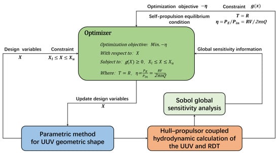
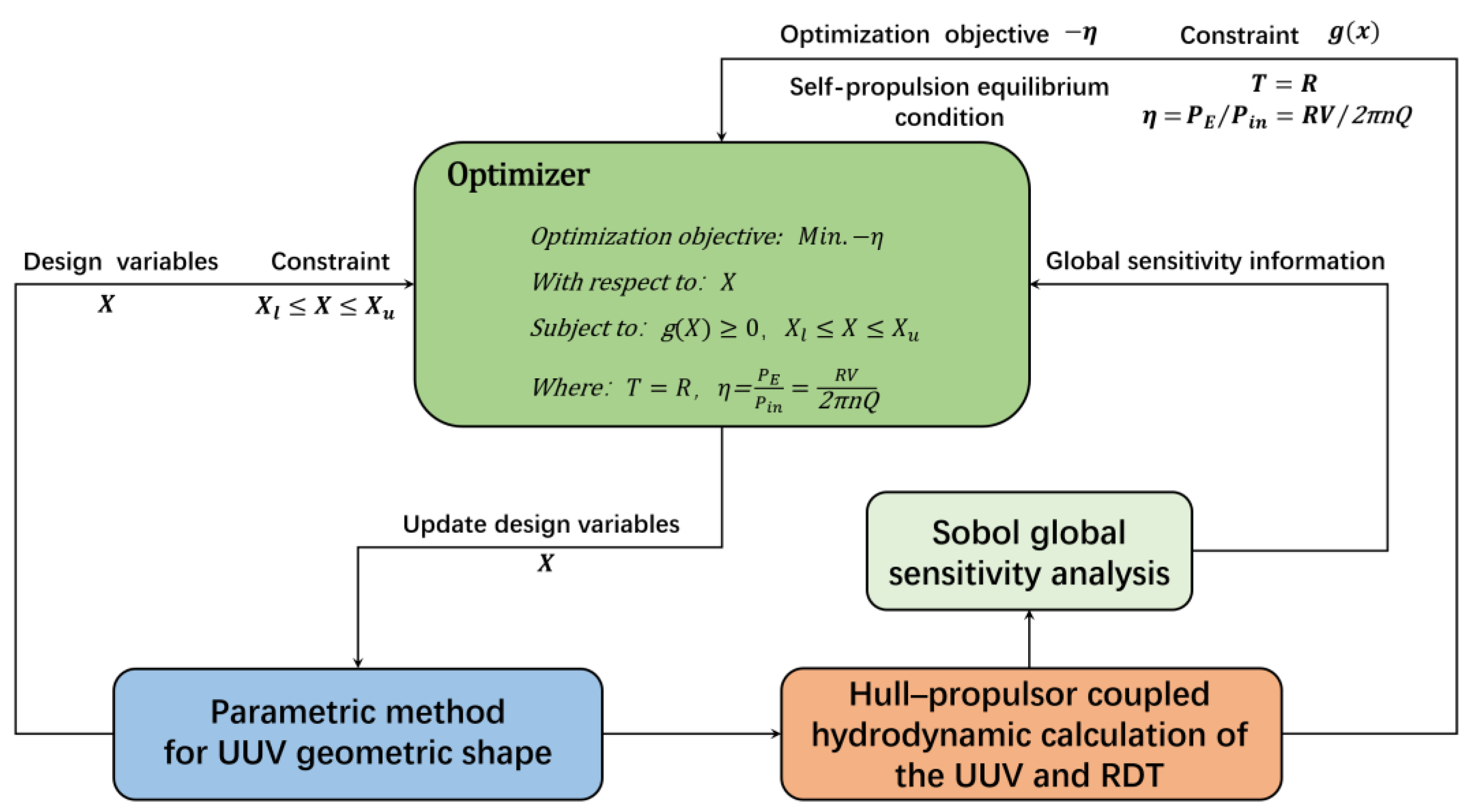
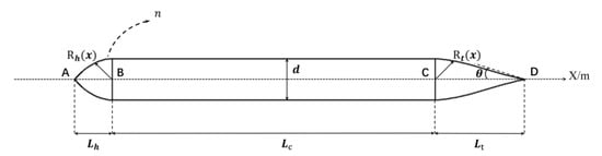
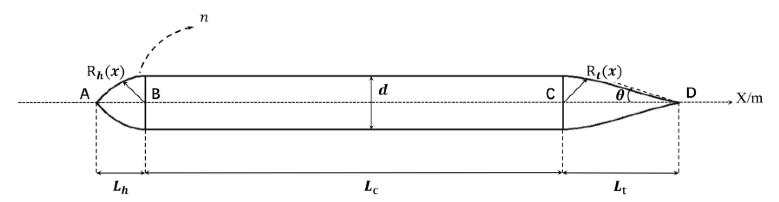
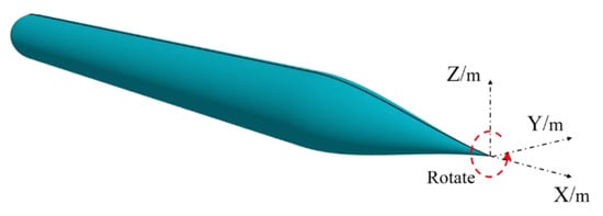
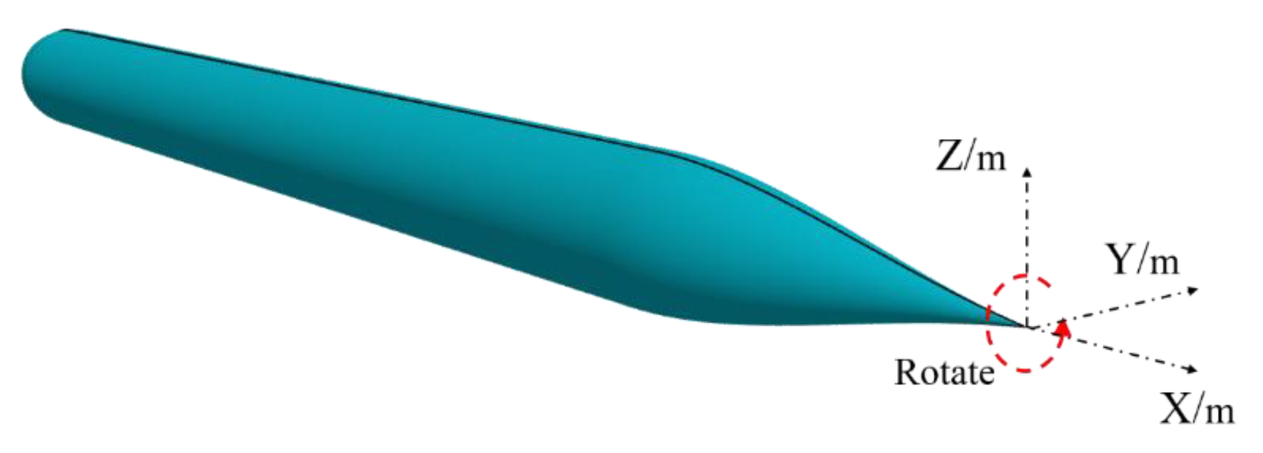
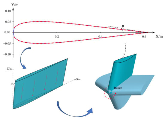
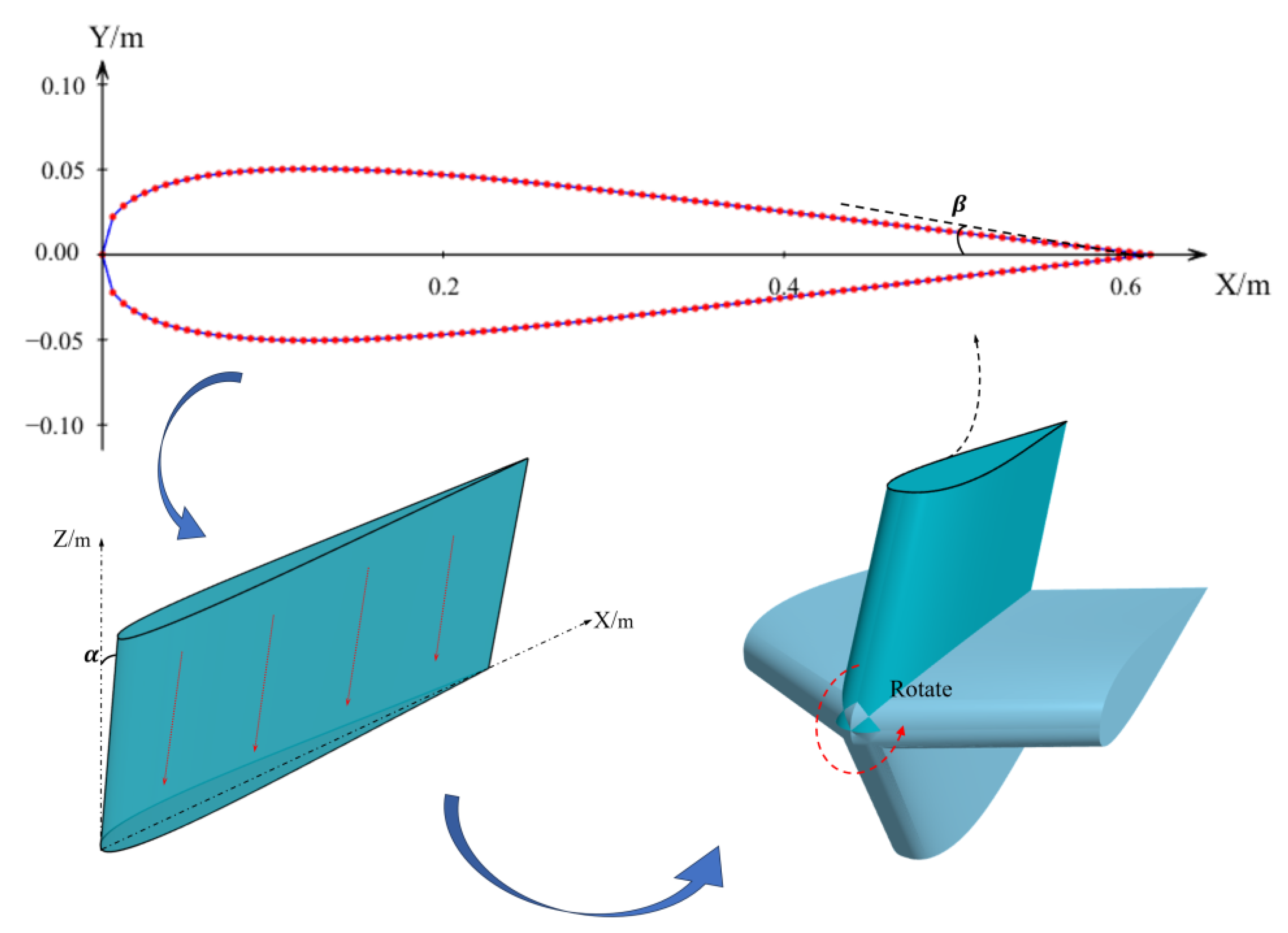
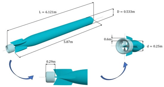
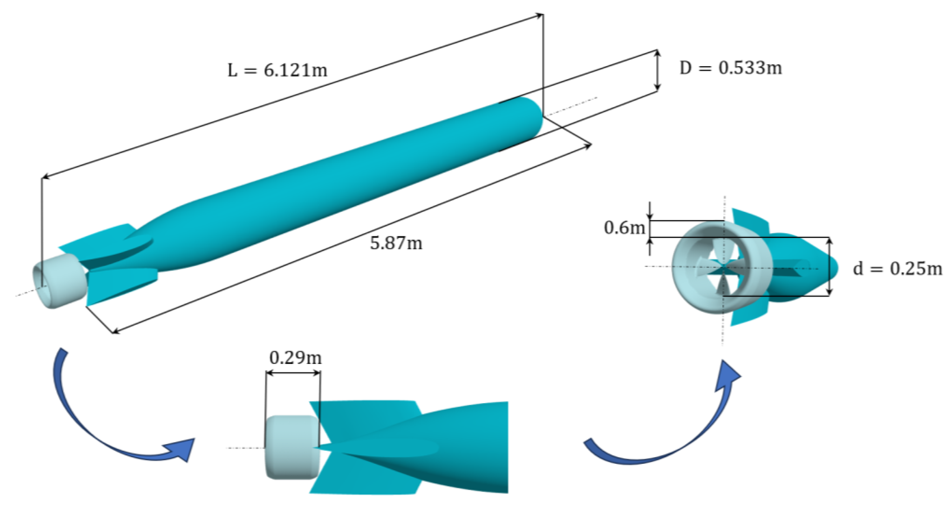
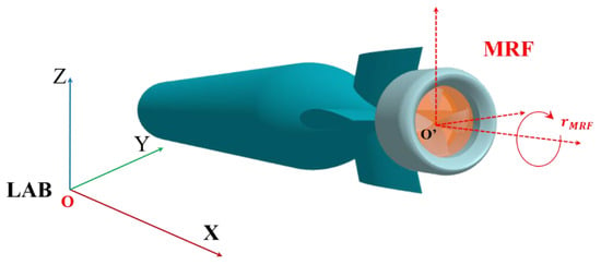
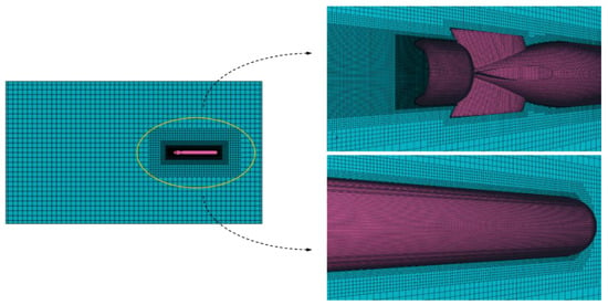
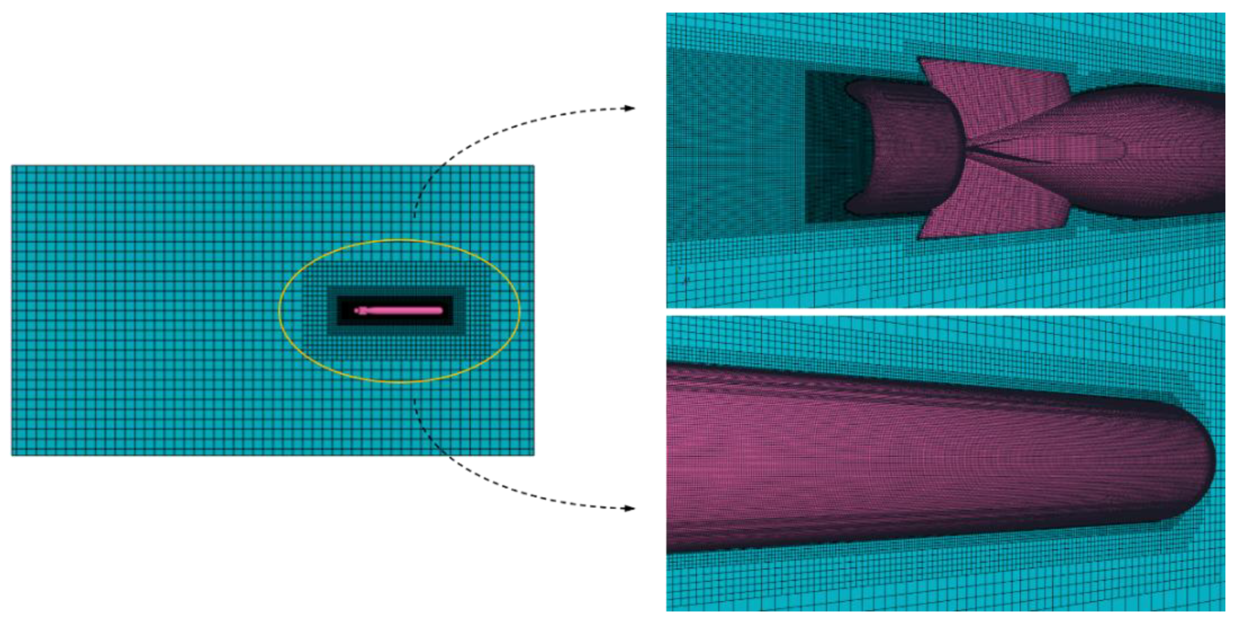
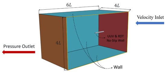
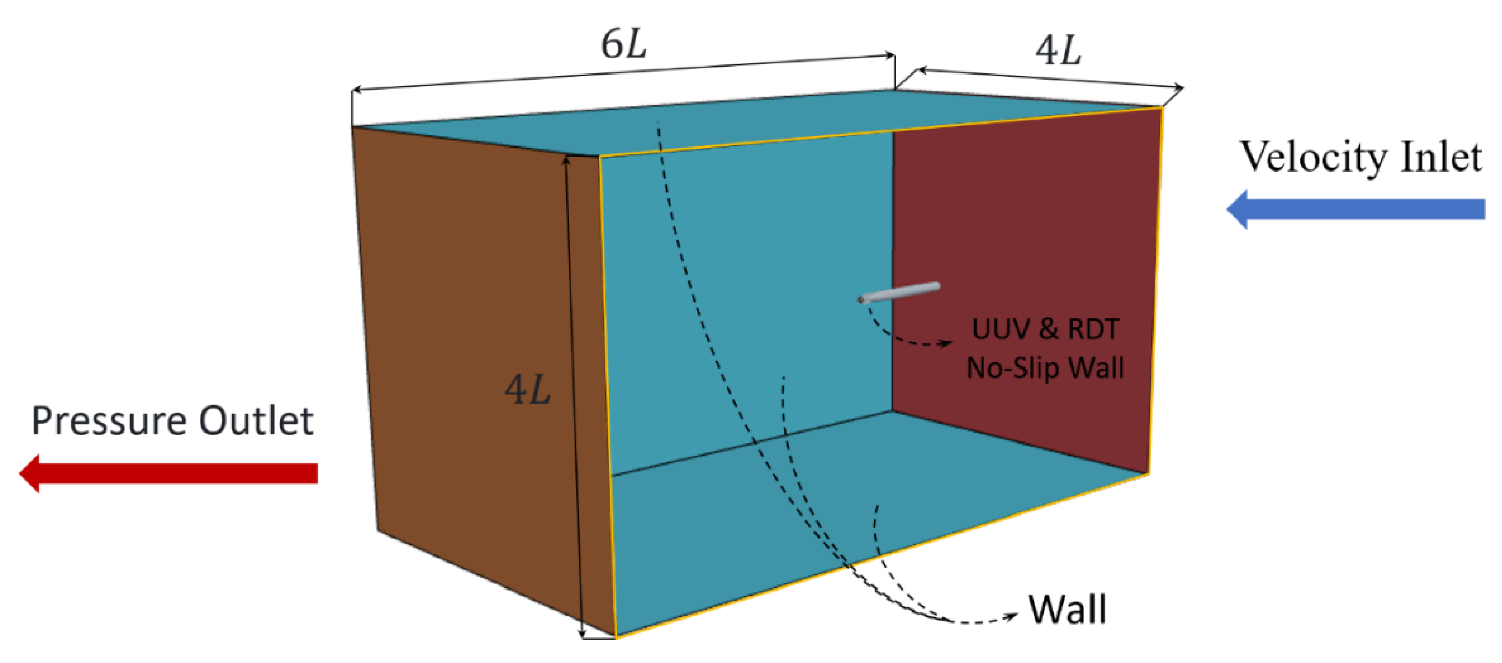
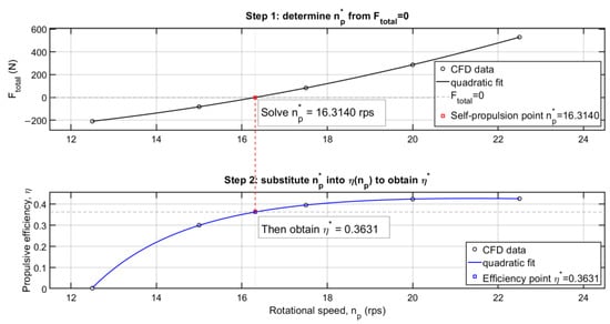
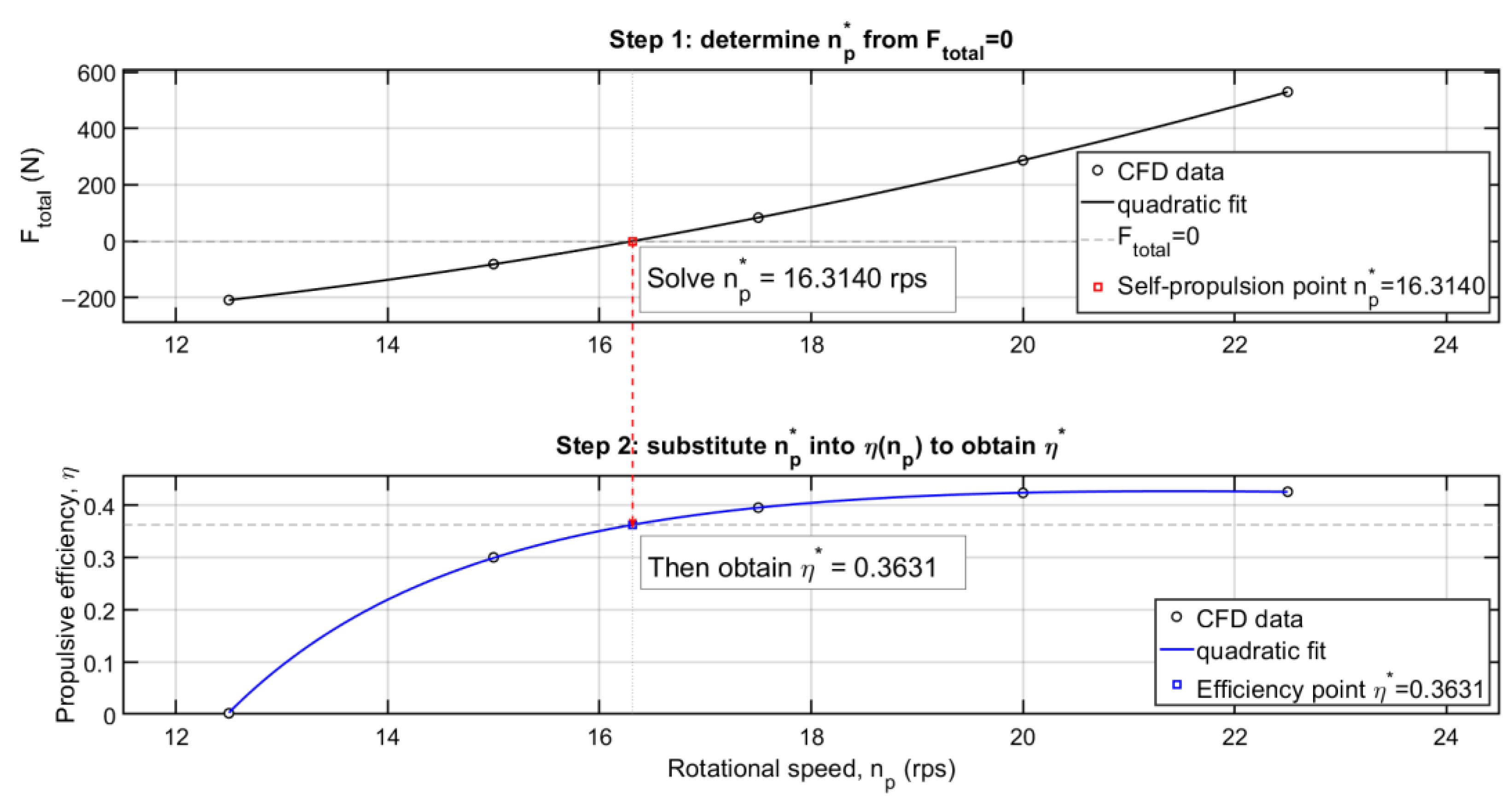
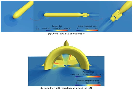
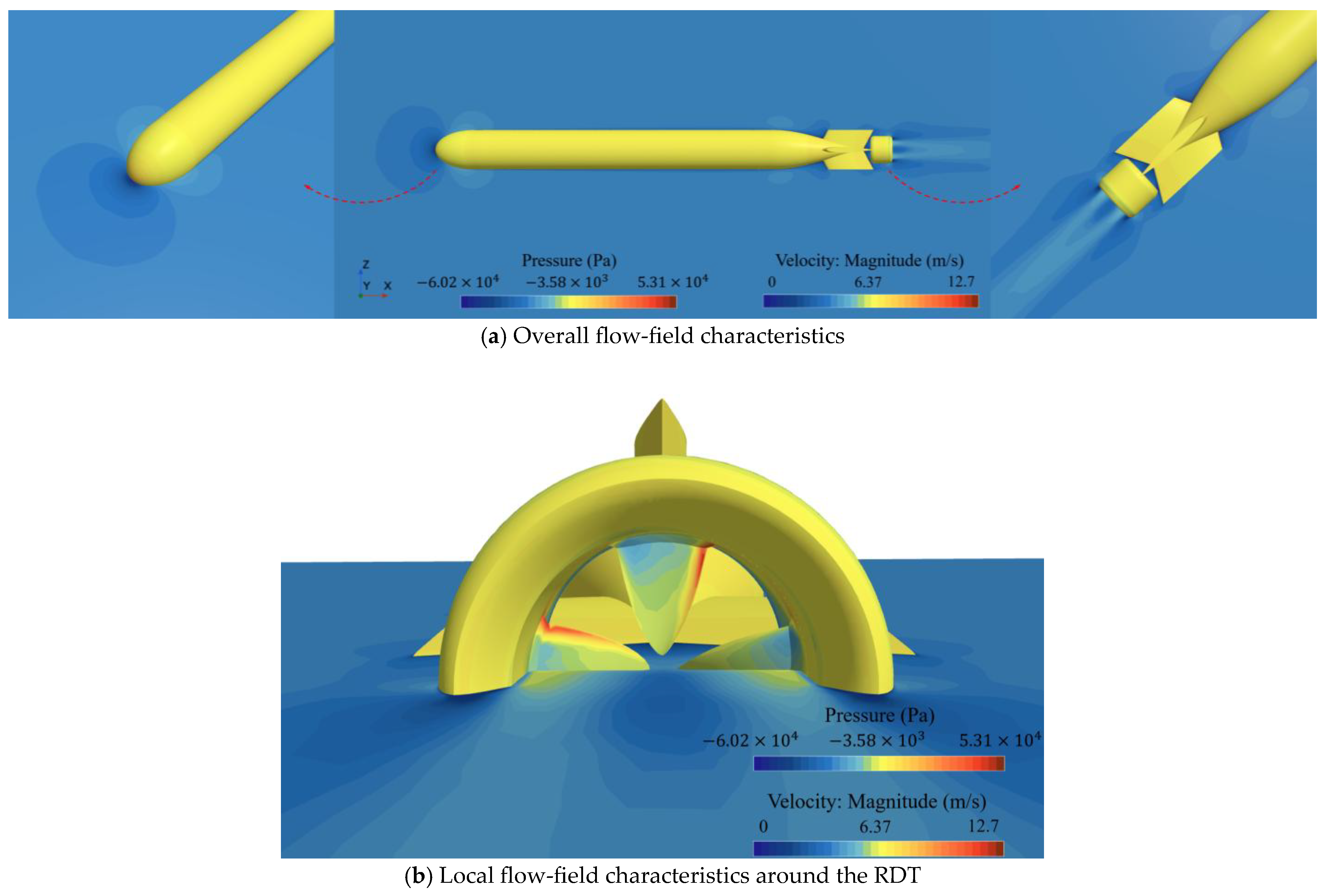
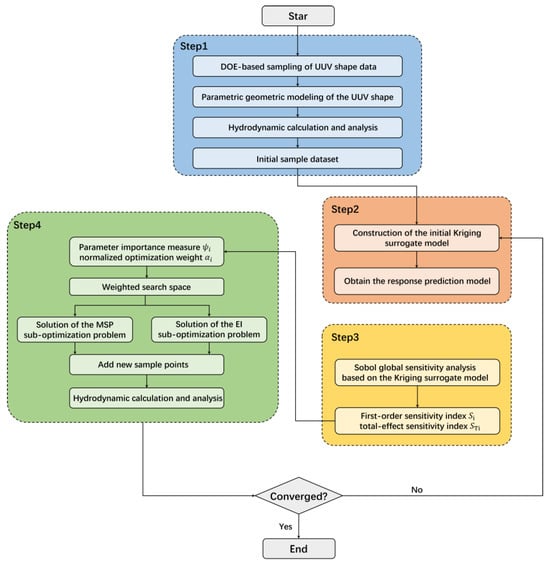
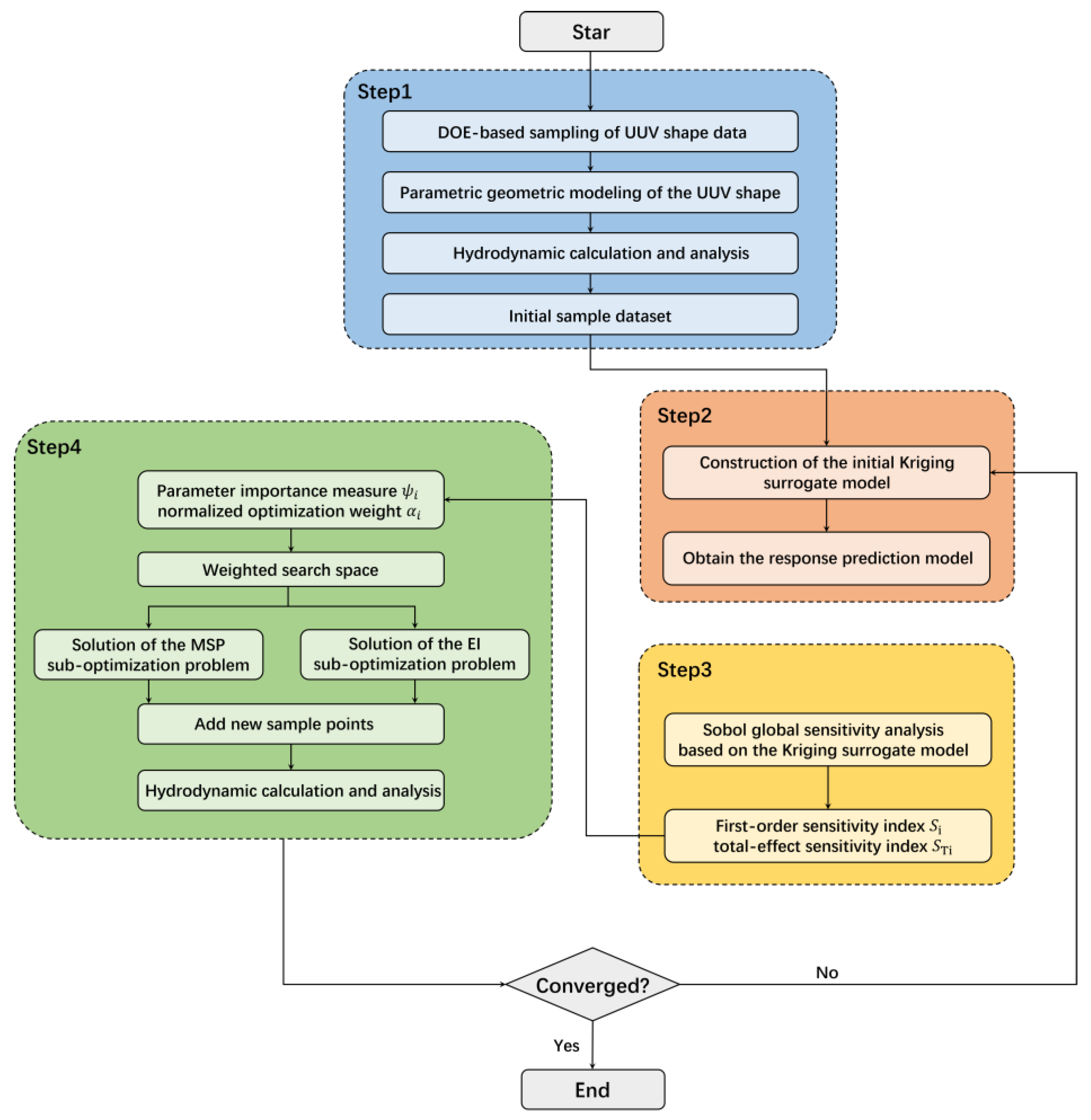
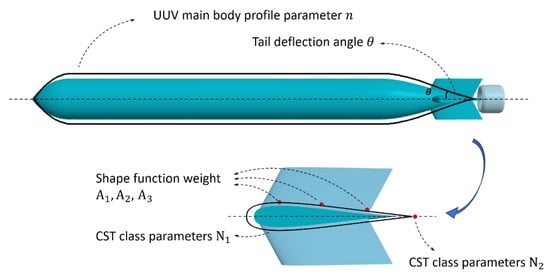
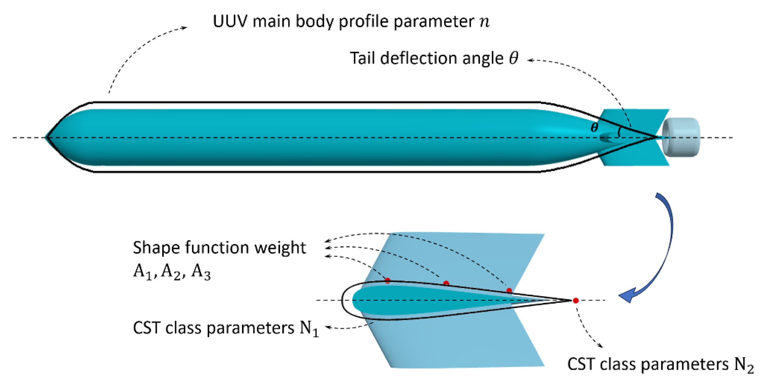
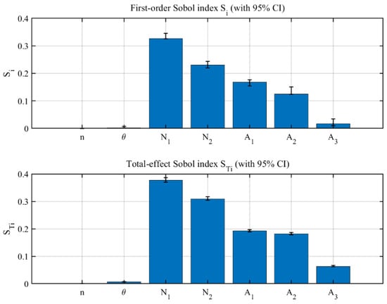
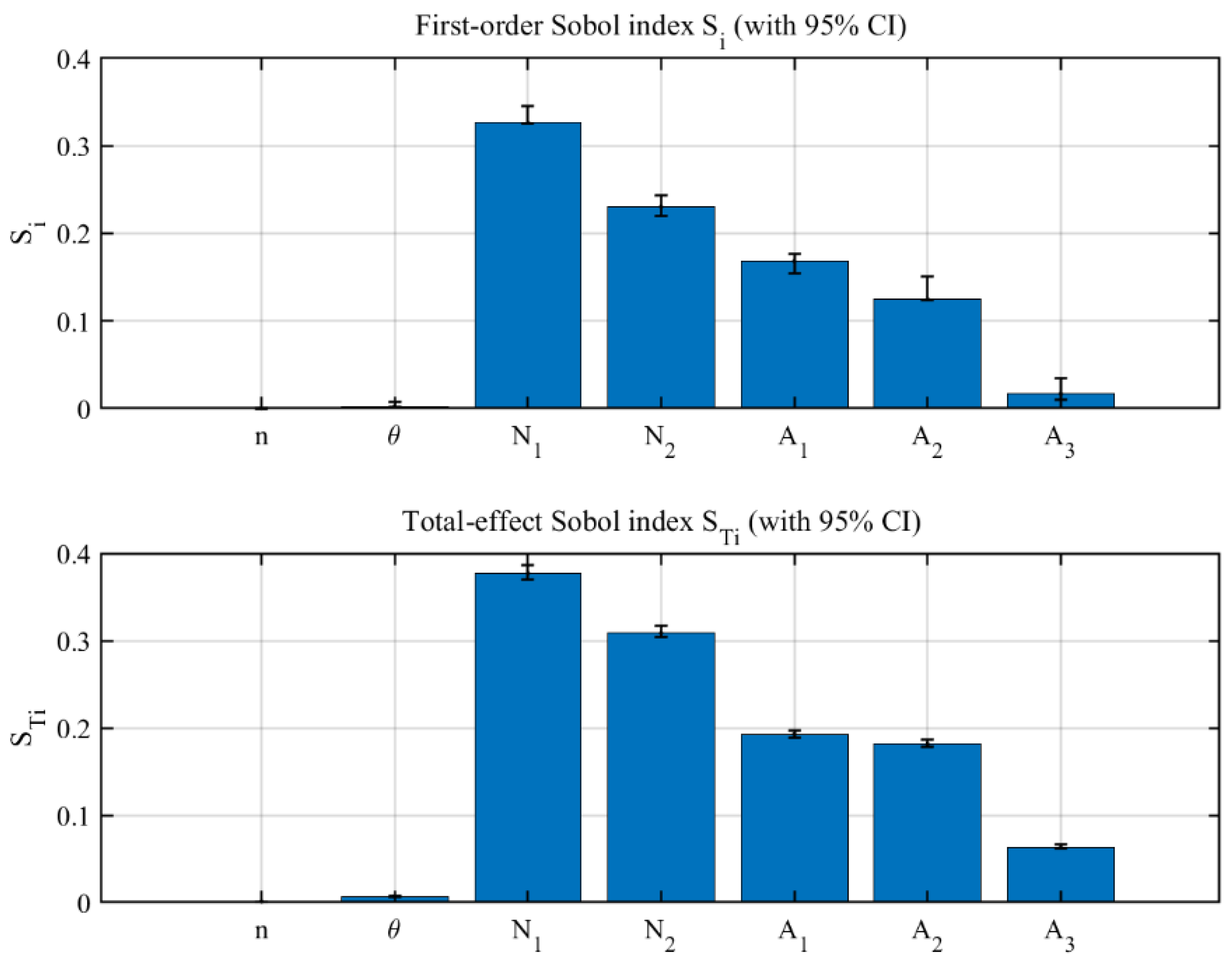
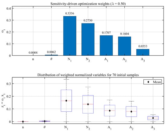
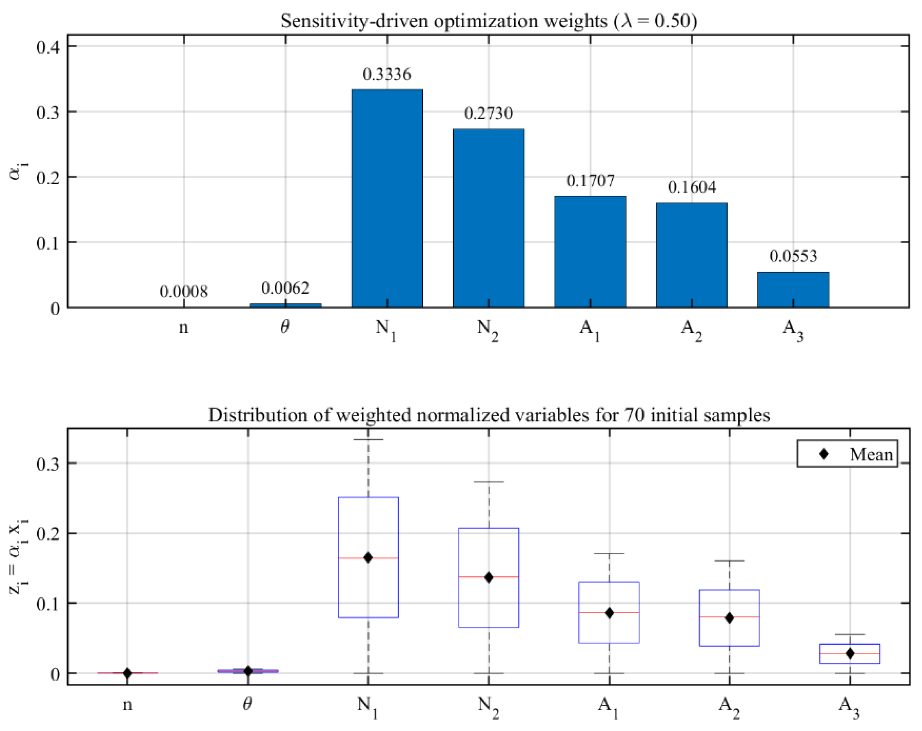
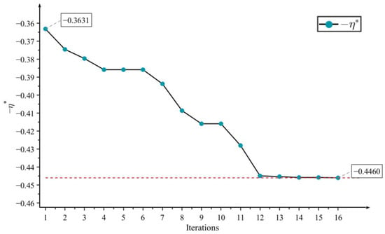
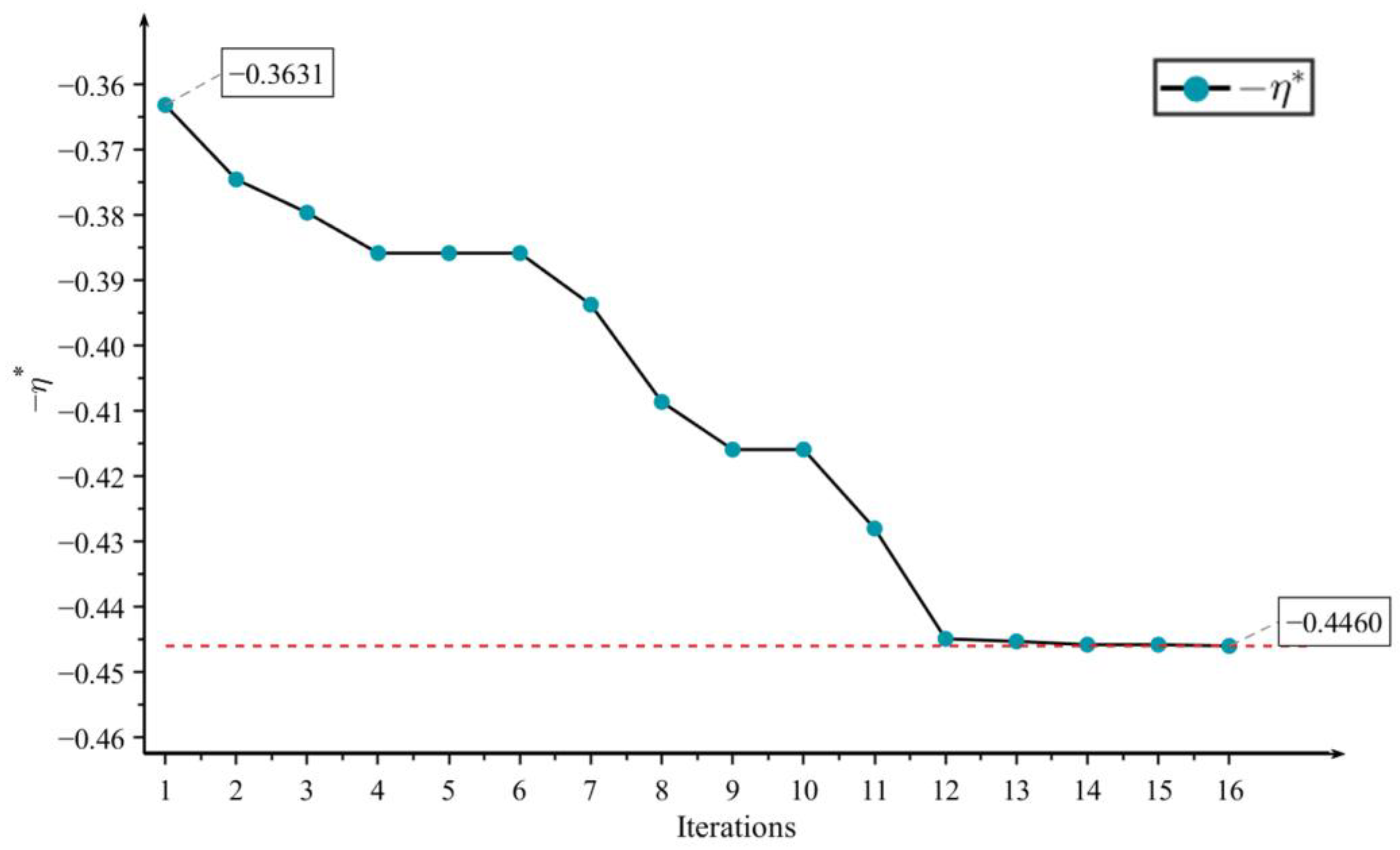
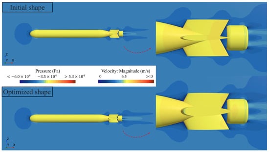
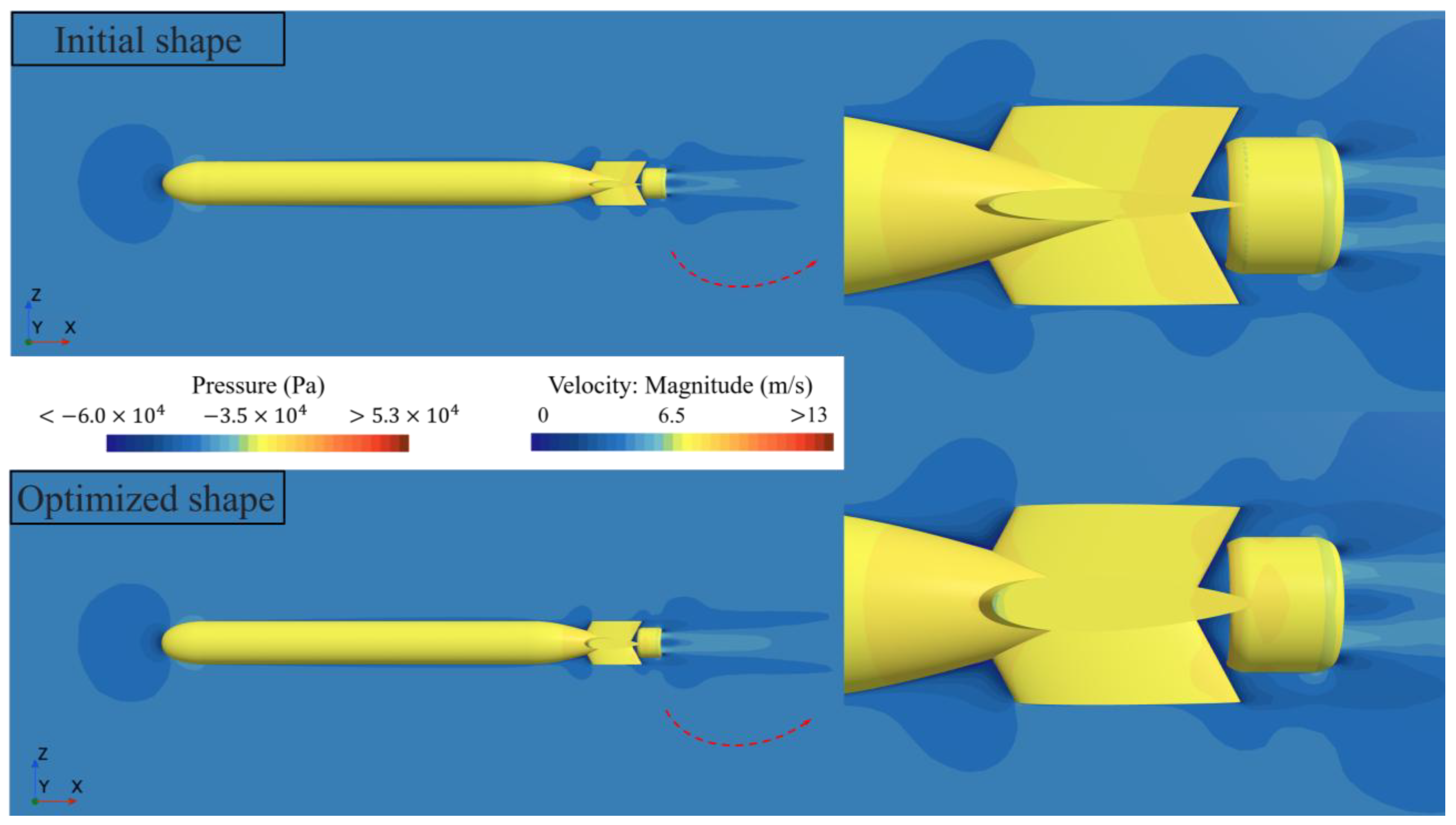
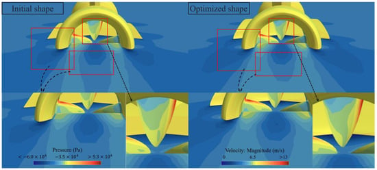
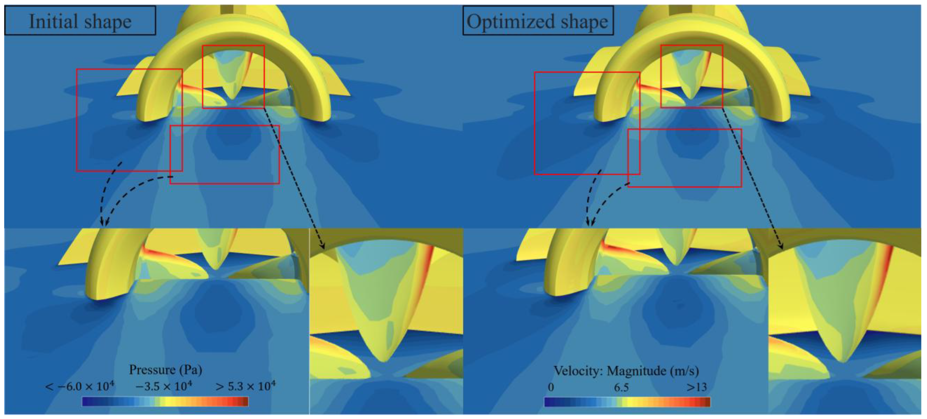
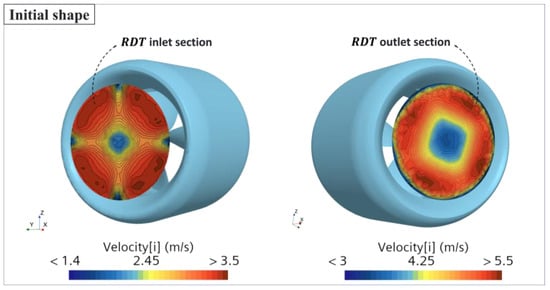
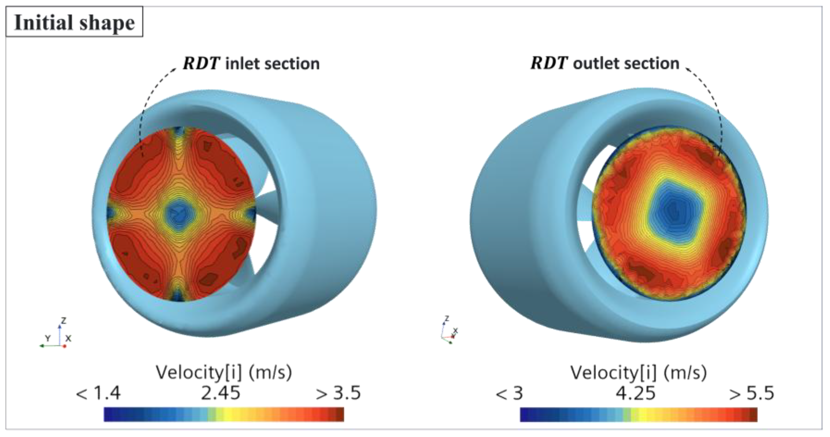
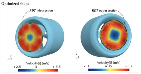
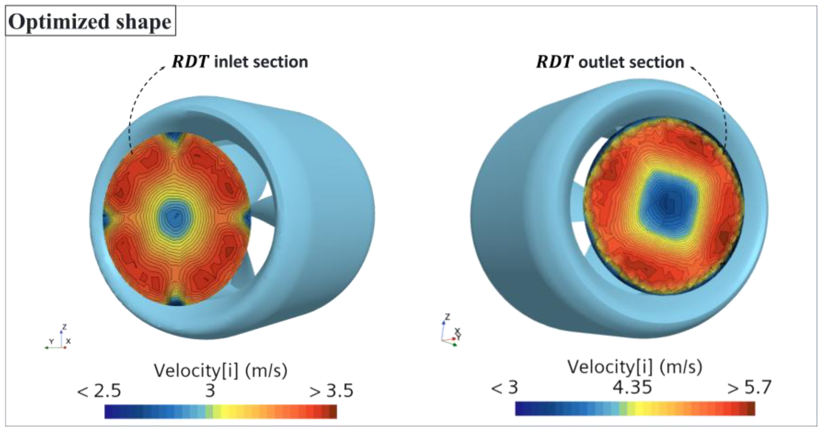

Disclaimer/Publisher’s Note: The statements, opinions and data contained in all publications are solely those of the individual author(s) and contributor(s) and not of MDPI and/or the editor(s). MDPI and/or the editor(s) disclaim responsibility for any injury to people or property resulting from any ideas, methods, instructions or products referred to in the content. |
© 2026 by the authors. Licensee MDPI, Basel, Switzerland. This article is an open access article distributed under the terms and conditions of the Creative Commons Attribution (CC BY) license.